Adaptively Perturbed Mirror Descent for Learning in Games
Abstract
This paper proposes a payoff perturbation technique for the Mirror Descent (MD) algorithm in games where the gradient of the payoff functions is monotone in the strategy profile space, potentially containing additive noise. The optimistic family of learning algorithms, exemplified by optimistic MD, successfully achieves last-iterate convergence in scenarios devoid of noise, leading the dynamics to a Nash equilibrium. A recent re-emerging trend underscores the promise of the perturbation approach, where payoff functions are perturbed based on the distance from an anchoring, or slingshot, strategy. In response, we propose Adaptively Perturbed MD (APMD), which adjusts the magnitude of the perturbation by repeatedly updating the slingshot strategy at a predefined interval. This innovation empowers us to find a Nash equilibrium of the underlying game with guaranteed rates. Empirical demonstrations affirm that our algorithm exhibits significantly accelerated convergence.
1 Introduction
This study delves into a variant of Mirror Descent (MD) (Nemirovskij & Yudin, 1983; Beck & Teboulle, 2003) in the context of monotone games whose gradient of the payoff functions exhibits monotonicity concerning the strategy profile space. This encompasses diverse games, including Cournot competition (Bravo et al., 2018), -cocoercive games (Lin et al., 2020), concave-convex games, and zero-sum polymatrix games (Cai & Daskalakis, 2011; Cai et al., 2016). Due to their extensive applicability, various learning algorithms have been developed and scrutinized to compute a Nash equilibrium efficiently.
Agents, which are prescribed to play according to MD or its variant, choose strategies with higher expected payoffs more likely but do not move far away from current strategies via regularization. The dynamics is known to converge to an equilibrium in an average sense, which is referred to as average-iterate convergence. In other words, the averaged strategy profile over iterations converges to an equilibrium. Nevertheless, research has shown that the actual trajectory of the updated strategy profiles fails to converge even in two-player zero-sum games and a specific class within monotone games (Mertikopoulos et al., 2018; Bailey & Piliouras, 2018). On the contrary, optimistic learning algorithms, incorporating recency bias, have shown success. The updated strategy profile itself converges to a Nash equilibrium (Daskalakis et al., 2018; Daskalakis & Panageas, 2019; Mertikopoulos et al., 2019; Wei et al., 2021), termed last-iterate convergence.
However, the optimistic approach faces challenges with feedback contaminated by some noise. Typically, each agent updates his or her strategy according to the perfect gradient feedback of the payoff function at each iteration, denoted as full feedback. In a more realistic scenario, noise might distort this feedback. With noisy feedback, optimistic learning algorithms perform suboptimally. For instance, Abe et al. (2023) empirically demonstrated that optimistic Multiplicative Weights Update (OMWU) fails to converge to an equilibrium, orbiting around it.
Alternatively, perturbation of payoffs has emerged again as a pivotal concept for achieving last-iterate convergence, even under noise (Abe et al., 2023). Payoff perturbation is a classical technique, as seen in Facchinei & Pang (2003), and introduces strongly convex penalties to the players’ payoff functions to stabilize learning. This leads to convergence to approximate equilibria, not only in the full feedback setting but also in the noisy feedback setting. However, to ensure convergence toward a Nash equilibrium of the underlying game, the magnitude of perturbation requires careful adjustment, which is calculated as the product of a strongly convex penalty function and a perturbation strength parameter. In fact, Liu et al. (2023) shrink the perturbation strength based on the current strategy profile’s proximity to an underlying equilibrium. Similarly, iterative Tikhonov regularization methods (Koshal et al., 2010; Tatarenko & Kamgarpour, 2019) adjust the magnitude of perturbation by using a sequence of perturbation strengths that satisfy certain conditions, such as diminishing as the iteration increases. Although these algorithms admit last-iterate convergence, it becomes challenging to choose an appropriate learning rate for the shrinking perturbation strength, which often leads to a failure in achieving rapid convergence for these algorithms and their variants.
In response to this, we adaptively determine the amount of the penalty from the distance between the current strategy and an anchoring, or slingshot strategy , while maintaining the perturbation strength parameter constant. Instead of carefully decaying the perturbation strength, the slingshot strategies are re-initialized at a predefined interval by the current strategies, and thus the magnitude of the perturbation is adjusted. To the best of our knowledge, Perolat et al. (2021) were the first to employ this idea and enabled Abe et al. (2023) to modify MWU to achieve last-iterate convergence. However, they have established the convergence only in an asymptotic manner. The significance of our work, in part, lies in extending these two studies and establishing non-asymptotic convergence results.
Our contributions are manifold. First, we identify our algorithm as Adaptively Perturbed MD111An implementation of our method is available at https://github.com/CyberAgentAILab/adaptively-perturbed-md (APMD). Second, we analyze the case where both the perturbation function and the proximal regularizer are assumed to be the squared -distance and provide the last-iterate convergence rates to a Nash equilibrium, and with full and noisy feedback, respectively. We also discuss the case where different distances from the squared -distance are utilized. Finally, we empirically reveal that our proposed APMD significantly outperforms MWU and OMWU in two zero-sum polymatrix games, regardless of the feedback type.
2 Preliminaries
Monotone games.
This paper focuses on a continuous game, which is denoted by . represents the set of players, represents the -dimensional compact convex strategy space for player , and we write . Each player chooses a strategy from and aims to maximize her differentiable payoff function . We write as the strategies of all players except player , and denote the strategy profile by . This study particularly considers a smooth monotone game, where the gradient of the payoff functions is monotone:
| (1) |
and -Lipschitz:
| (2) |
where is the -norm.
Monotone games include many common and well-studied classes of games, such as concave-convex games, zero-sum polymatrix games, and Cournot competition.
Example 2.1 (Concave-Convex Games).
Let us consider a max-min game , where . Player aims to maximize , while player aims to minimize . If is concave in and convex in , the game is called a concave-convex game or minimax optimization problem, and it is easy to confirm that the game is monotone.
Example 2.2 (Zero-Sum Polymatrix Games).
In a zero-sum polymatrix game, each player’s payoff function can be decomposed as , where is represented by with some matrix , and satisfies . In this game, each player can be interpreted as playing a two-player zero-sum game with each other player . From the linearity and zero-sum property of , we can easily show that . Thus, the zero-sum polymatrix game is a special case of monotone games.
Nash equilibrium and gap function.
A Nash equilibrium (Nash, 1951) is a common solution concept of a game, which is a strategy profile where no player can improve her payoff by deviating from her specified strategy. Formally, a Nash equilibrium satisfies the following condition:
We denote the set of Nash equilibria by . Note that a Nash equilibrium always exists for any smooth monotone game (Debreu, 1952). Furthermore, we measure the proximity to Nash equilibrium for a given strategy profile by its gap function, which is defined as:
The gap function is a standard metric of proximity to Nash equilibrium for a given strategy profile (Cai & Zheng, 2023). From the definition, for any , and the equality holds if and only if is a Nash equilibrium.
Problem setting.
In this study, we consider the online learning setting where the following process is repeated for iterations: 1) At each iteration , each player chooses her strategy based on the previously observed feedback; 2) Each player receives the gradient feedback as feedback. This study considers two feedback models: full feedback and noisy feedback. In the full feedback setting, each player receives the perfect gradient vector as feedback, i.e., . In the noisy feedback setting, each player’s feedback is given by , where is a noise vector. Specifically, we focus on the zero-mean and bounded-variance noise vectors.
Mirror Descent.
Mirror Descent (MD) is a widely used algorithm for learning equilibria in games. Let us define as the strictly convex regularization function and as the associated Bregman divergence. Then, MD updates each player ’s strategy at iteration as follows:
where is the learning rate at iteration .
Other notations.
We denote a -dimensional probability simplex by . We define as the diameter of . The Kullback-Leibler (KL) divergence is defined by . Besides, with a slight abuse of notation, we represent the sum of Bregman divergences and the sum of KL divergences by , and , respectively. We finally denote the domain of by , and corresponding interior by .
3 Adaptively Perturbed Mirror Descent
In this section, we present Adaptively Perturbed Mirror Descent (APMD), which is an extension of the standard MD algorithms. Algorithm 1 describes the pseudo-code. APMD employs two pivotal techniques: slingshot payoff perturbation and slingshot strategy update. Each of them corresponds to line 5 and line 9 in Algorithm 1, respectively.

3.1 Slingshot Payoff Perturbation
Letting us define the differentiable divergence function and the slingshot strategy , APMD perturbs each player’s payoff by the divergence between the current strategy and the slingshot strategy , i.e., . Specifically, APMD updates each player’s strategy according to
| (3) |
where is the perturbation strength and denotes differentiation with respect to first argument. We assume that is strictly convex for every , and takes a minimum value of at . Furthermore, we assume that is differentiable and -strongly convex on with .
The conventional MD updates its strategy based on the gradient feedback of the payoff function and the regularization term. The regularization term adjusts the next strategy so that it does not deviate significantly from the current strategy. APMD perturbs the gradient payoff vector by the divergence between the current strategy and a predefined slingshot strategy . If the current strategy is far away from the slingshot strategy, the magnitude of the perturbation increases. Note that if both strategies are equivalent, no perturbation occurs, and APMD just seeks a strategy with a higher expected payoff. As Figure 1 illustrates, the divergence first fluctuates, and then the current strategy profile comes close to a stationary point where the gradient of the expected payoff vector is equal to the gradient of the magnitude of the perturbation so that the perturbation via slingshot stabilizes the learning dynamics. Indeed, Mutant Follow the Regularized Leader (Mutant FTRL) instantiated in Example 5.3 encompasses replicator-mutator dynamics, which is guaranteed to converge to an approximate equilibrium in two-player zero-sum games (Abe et al., 2022). We can argue that APMD inherits this nice feature.
3.2 Slingshot Strategy Update
The perturbation via slingshot enables to converge quickly to a stationary point (Lemmas 5.6 and 5.7). Different slingshot strategy profiles induce different stationary points. Of course, when the slingshot strategy profile is set to be an equilibrium, the corresponding stationary point also becomes an equilibrium. However, it is virtually impossible to identify such an ideal slingshot strategy profile beforehand. To this end, APMD adjusts a slingshot strategy profile by replacing it with the (nearly) stationary point that is reached after predefined iterations .
Figure 1 illustrates how our slingshot strategy update brings the corresponding stationary points closer to an equilibrium. x- and y-axis indicate the number of iterations and the logarithm of the gap function of the last-iterate strategy profile. We here assume that the learning rate and the perturbation strength are and , respectively. The initial slingshot strategy is given as a uniform distribution on the action space. After the first interval of iterations, APMD finds a stationary point. The slingshot strategy profile for the second interval is replaced with the stationary point. Figure 1 clearly shows the stationary point, i.e., the last-iterate strategy profile comes close to an equilibrium every time the slingshot strategy profile is updated. We also theoretically justify our slingshot strategy update in Theorem D.1, i.e., when the slingshot strategy profile is close to an equilibrium , the stationary point is close to .
4 Last-Iterate Convergence Rates
In this section, we establish the last-iterate convergence rates of APMD. More specifically, we examine a setting where both and is set to the squared -distance, i.e., . This instance can be considered as an extended version of Gradient Descent, which incorporates our techniques of payoff perturbation and slingshot strategy update. We also assume that the gradient vector of is bounded. We emphasize that we have obtained the overall last-iterative convergence rates of APMD for the entire iterations in both full and noisy feedback settings.
4.1 Full Feedback Setting
First, we demonstrate the last-iterate convergence rate of APMD with full feedback where each player receives the perfect gradient vector , at each iteration . Theorem 4.1 provides the APMD’s convergence rate of in terms of the gap function. Note that the learning rate is constant, and its upper bound is specified by perturbation strength and smoothness parameter .
Theorem 4.1.
If we use the constant learning rate , and set and as the squared -distance , and set , then the strategy profile updated by APMD satisfies:
The obtained rate herein is competitive with optimistic gradient and extra-gradient methods (Cai et al., 2022a) whose rates are . Although it is open whether our convergence rate matches its lower bound, it closely aligns with the lower bound for the class of algorithms that includes -SCLI algorithms (Golowich et al., 2020b), which is different from our APMD. To the best of our knowledge, the fastest rate of is achieved by Accelerated Optimistic Gradient (AOG) (Cai & Zheng, 2023), which is an optimistic variant of the Halpern iteration (Halpern, 1967). At first sight, the update rule of AOG looks as if the perturbation strength was linearly decayed. However, it does not perturb the payoff functions and instead adjusts the regularization term by using the convex combination of the current strategy and the anchoring strategy as the proximal point in MD. Unlike our APMD, the anchoring strategy is never updated through the iterations.222Regarding the rate of , a companion paper is in preparation.
4.2 Proof Sketch of Theorem 4.1
This section sketches the proof for Theorem 4.1. We present the complete proofs for the theorem and associated lemmas in Appendix E.
(1) Convergence rates to a stationary point with -th slingshot strategy profile.
We denote as the slingshot strategy profile after updates. Since the slingshot strategy profile is overwritten by the current strategy profile every iterations, we can write . We first prove that, as increases, the next -th slingshot strategy profile approaches to the stationary point under the slingshot strategy profile , which satisfies the following condition: ,
| (4) |
Note that always exists since the perturbed game is still monotone. Using the strong convexity of , we show that as :
Lemma 4.2.
Assume that and are set as the squared -distance. If we use the constant learning rate , the -th slingshot strategy profile of APMD under the full feedback setting satisfies that:
(2) Upper bound on the gap function.
Next, we derive the upper bound on the gap function for . From the bounding technique of the gap function using the tangent residuals by Cai et al. (2022a) and the first-order optimality condition for , the gap function for can be upper bounded by the distance between the slingshot strategy profile and the stationary point :
Lemma 4.3.
If is set as the squared -distance, the gap function for of APMD satisfies for :
By Lemma 4.2, if we set as the squared -distance, the first term in this lemma can be bounded as:
| (5) |
Therefore, it is enough to derive the convergence rate on the -distance between and .
(3) Last-iterate convergence results for the slingshot strategy profile.
Let us denote as the total number of the slingshot strategy updates over the entire iterations. Then, by adjusting , we show that the -distance between the -th slingshot strategy profile and the corresponding stationary point decreases as increases:
Lemma 4.4.
In the same setup of Theorem 4.1, the -th slingshot strategy profile of APMD satisfies:
Lemma 4.4 implies that as increases, the variation of becomes negligible, signifying convergence in its behavior.
4.3 Noisy Feedback Setting
Next, we consider the noisy feedback setting, where each player receives a gradient vector with additive noise: . Define the sigma-algebra generated by the history of the observations: , . We assume that the noise vectors are with zero-mean and bounded variances. We also suppose that the noise vectors are independent over . In this setting, the last-iterate convergence rate is achieved by APMD using a decreasing learning rate sequence . The convergence rate obtained by APMD is :
Theorem 4.5.
Let and . Assume that and are set as the squared -distance , and . If we choose the learning rate sequence of the form , then the strategy profile updated by APMD satisfies:
It should be noted that Theorem 4.5 provides a non-asymptotic convergence guarantee with a rate. This is a significant departure from the existing convergence results (Koshal et al., 2010, 2013; Tatarenko & Kamgarpour, 2019), which focus on the asymptotic convergence of iterative Tikhonov regularization methods in the noisy or bandit feedback settings.
4.4 Proof Sketch of Theorem 4.5
As in Theorem 4.1, we first derive the convergence rate of for the noisy feedback setting:
Lemma 4.6.
Let and . Suppose that both and are defined as the squared -distance. Under the noisy feedback setting, if we use the learning rate sequence of the form , the -th slingshot strategy profile of APMD for each satisfies that:
The proof is given in Appendix E.6 and is based on the standard argument of stochastic optimization, e.g., Nedić & Lee (2014). However, the proof is made possible by taking into account the monotonicity of the game and the relative (strong and smooth) convexity of the divergence function.
Next, in a similar manner for Lemma 4.4, we show the upper bound on the expected distance between and under the noisy feedback setting:
Lemma 4.7.
In the same setup of Theorem 4.5, the -th slingshot strategy profile satisfies:
5 Beyond Squared -Payoff Perturbation
Section 4 assumes that both and are the squared -distance. This section considers more general choices of and .
5.1 Instantiation of Payoff-Perturbed Algorithms
First, we would like to emphasize that choosing appropriate combinations of and enables APMD to reproduce some existing learning algorithms that incorporate payoff perturbation. For example, the following learning algorithms can be viewed as instantiations of APMD.
Example 5.1 (Boltzmann Q-Learning (Tuyls et al., 2006)).
Assume that , the regularize is entropy: . Let us set as the KL divergence and the slingshot strategy as a uniform distribution, i.e., and . Then, the corresponding continuous-time APMD dynamics can be expressed as:
which is equivalent to Boltzman Q-learning (Tuyls et al., 2006; Bloembergen et al., 2015).
Example 5.2 (Reward transformed FTRL (Perolat et al., 2021)).
5.2 Convergence Results with General and
Next, we establish the convergence results for APMD with general combinations of and . For theoretical analysis, we assume a specific condition on :
Assumption 5.4.
is differentiable over . Moreover, is -smooth and -strongly convex relative to , i.e., for any , holds.
Note that these assumptions are always satisfied with whenever is identical to ; thus, these are not strong assumptions. We also assume that is well-defined over iterations:
Assumption 5.5.
updated by APMD satisfies for any .
Lemma 5.6.
Lemma 5.7.


These lemmas imply that as . Therefore, when is sufficiently large, -th slingshot strategy profile becomes almost equivalent to the stationary point . From this, we anticipate that as even in the noisy feedback setting. The subsequent theorems provide asymptotic last-iterate convergence results for this ideal scenario. In particular, we show that the slingshot strategy profile converges to equilibrium when using the following divergence functions as : 1) Bregman divergence; 2) -divergence; 3) Rényi-divergence; 4) reverse KL divergence.
Theorem 5.8.
Assume that is a Bregman divergence for some strongly convex function , and for . Then, there exists such that as .
Theorem 5.9.
Let us define . Assume that for , and is one of the following divergence: 1) -divergence with ; 2) Rényi-divergence with ; 3) reverse KL divergence. If the initial slingshot strategy profile is in the interior of , the sequence converges to the set of Nash equilibria of the underlying game.
6 Experiments
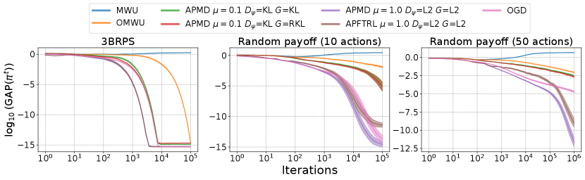
This section empirically compares the representative instance of MD, namely Multiplicative Weight Update (MWU) and its Optimistic version (OMWU), with our framework. Specifically, we consider the following three instances of APMD: (i) both are the squared -distance; (ii) both and are the KL divergence, which is also an instance of Reward transformed FTRL in Example 5.2. Note that if the slingshot strategy is fixed to a uniformly random strategy, this algorithm corresponds to Boltzmann Q-Learning in Example 5.1; (iii) the divergence function is the reverse KL divergence, and the Bregman divergence is the KL divergence, which matches Mutant FTRL in Example 5.3.
We focus on two zero-sum polymatrix games: Three-Player Biased Rock-Paper-Scissors (3BRPS) and three-player random payoff games with and actions. For the 3BRPS game, each player participates in two instances of the game in Table 2 in Appendix I simultaneously with two other players. For the random payoff games, each player participates in two instances of the game with two other players simultaneously. The payoff matrix for each instance is denoted as . Each entry of is drawn independently from a uniform distribution on the interval .
Figures 2 and 3 illustrate the logarithm of the gap function averaged over instances with different random seeds. We assume that the initial slingshot strategy profile is chosen uniformly at random in the interior of the strategy space in each instance for 3BRPS, while is chosen as for in every instances for the random payoff games.
First, Figure 2 depicts the case of full feedback. Unless otherwise specified, we use a constant learning rate and a perturbation strength for APMD. Further details and additional experiments can be found in Appendix I. Figure 2 shows that APMD outperforms MWU and OMWU in all three games. Notably, APMD exhibits the fastest convergence in terms of the gap function when using the squared -distance as both and . Next, Figure 3 depicts the case of noisy feedback. We assume that the noise vector is generated from the multivariate Gaussian distribution in an i.i.d. manner. To account for the noise, we use a lower learning rate than the full feedback case. In OMWU, we use the noisy gradient vector at the previous step as the prediction vector for the current iteration . We observe the same trends as with full feedback. While MWU and OMWU exhibit worse performance, APMD maintains its fast convergence, as predicted by the theoretical analysis.
7 Related Literature
Recent progress in achieving no-regret learning with full feedback has been driven by optimistic learning (Rakhlin & Sridharan, 2013a, b). Optimistic versions of well-known algorithms like Follow the Regularized Leader (Shalev-Shwartz & Singer, 2006) and Mirror Descent (Zhou et al., 2017; Hsieh et al., 2021) have been proposed to admit last-iterate convergence in a wide range of game settings. These optimistic algorithms have been successfully applied to various classes of games, including bilinear games (Daskalakis et al., 2018; Daskalakis & Panageas, 2019; Liang & Stokes, 2019; de Montbrun & Renault, 2022), cocoercive games (Lin et al., 2020), and saddle point problems (Daskalakis & Panageas, 2018; Mertikopoulos et al., 2019; Golowich et al., 2020b; Wei et al., 2021; Lei et al., 2021; Yoon & Ryu, 2021; Lee & Kim, 2021; Cevher et al., 2023). The advancements have provided solutions to monotone games and have established convergence rates (Golowich et al., 2020a; Cai et al., 2022a, b; Gorbunov et al., 2022; Cai & Zheng, 2023).
The exploration of literature with noisy feedback poses significant challenges, in contrast to full feedback. In situations where feedback is imprecise or limited, algorithms must estimate action values at each iteration. There have been two trends in achieving last-iterate convergence: restricting the class of games and perturbing the payoff functions. On one hand, particularly noticeable works lie in potential games (Cohen et al., 2017), normal-form games with strict Nash equilibria (Giannou et al., 2021b, a), and two-player zero-sum games (Abe et al., 2023). Also, noisy feedback is handled with games whose payoff functions are assumed to be strictly (or strongly) monotone (Bravo et al., 2018; Kannan & Shanbhag, 2019; Hsieh et al., 2019; Anagnostides & Panageas, 2022), while to be strictly variational stable (Mertikopoulos & Zhou, 2019; Mertikopoulos et al., 2019, 2022; Azizian et al., 2021). Note that variationally stable games, often referred to in control theory, are a slightly broader class of monotone games. These studies require the payoff functions to be strictly or strongly convex. When these restrictions are not imposed, convergence is primarily guaranteed only in an asymptotic sense, and the rate is not quantified (Hsieh et al., 2020, 2022).
On the other hand, payoff-perturbed algorithms have recently regained attention for their ability to demonstrate convergence in unrestricted games when noise is present. As described in Section 1, payoff perturbation is a textbook technique (Facchinei & Pang, 2003) that has been extensively studied (Koshal et al., 2010, 2013; Yousefian et al., 2017; Tatarenko & Kamgarpour, 2019; Abe et al., 2023; Cen et al., 2021, 2023; Cai et al., 2023; Pattathil et al., 2023). It is known that carefully adjusting the magnitude of perturbation ensures convergence to a Nash equilibrium. This magnitude is computed as the product of a strongly convex penalty and a perturbation strength parameter. Liu et al. (2023) shrink the perturbation strength based on a predefined hyper-parameter and the gap function of the current strategy. Likewise, Koshal et al. (2010) and Tatarenko & Kamgarpour (2019) have identified somewhat complex conditions that the sequence of the perturbation strength parameters and learning rates should satisfy. Roughly speaking, as we have implied in Lemma 4.2, a smaller strength would require a lower learning rate. This potentially decelerates the convergence rate and complicates the task of finding an appropriate learning rate. For practicality, we have opted to keep the perturbation strength constant, independent of the iteration in APMD. Moreover, it must be emphasized that the existing literature has primarily provided asymptotic convergence results, while we have successfully provided the non-asymptotic convergence rate.
Finally, the idea of the slingshot strategy update was initiated by Perolat et al. (2021) and later extended by Abe et al. (2023). Our contribution partly owes to the significance of quantifying the convergence rate for the first time. We must also mention that Sokota et al. (2023) have proposed a very similar, but essentially different update rule to ours. It just adds an additional regularization term based on an anchoring strategy, which they call a magnetic one, and this means that it directly perturbs the (expected) payoff functions. In contrast, our APMD indirectly perturbs the payoff functions, i.e., perturbs the gradient vector. Furthermore, we have established non-asymptotic convergence results toward a Nash equilibrium, while Sokota et al. (2023) have only shown convergence toward a quantal response equilibrium (McKelvey & Palfrey, 1995, 1998), which is just equivalent to an approximate equilibrium. Similar results to them have been obtained with the Boltzmann Q-learning dynamics (Tuyls et al., 2006) and penalty-regularized dynamics (Coucheney et al., 2015) in continuous-time settings (Leslie & Collins, 2005; Hussain et al., 2023).
8 Conclusion
This paper proposes a novel variant of MD that achieves last-iterate convergence even when the noise is present, by adaptively adjusting the magnitude of the perturbation. This research could lead to several intriguing future studies, such as finding the best perturbation strength for the optimal convergence rate and achieving convergence with more limited feedback, for example, using bandit feedback (Bravo et al., 2018; Drusvyatskiy et al., 2022).
Acknowledgments
Kaito Ariu is supported by JSPS KAKENHI Grant Number 23K19986. Atsushi Iwasaki is supported by JSPS KAKENHI Grant Numbers 21H04890 and 23K17547.
Impact Statement
This paper focuses on discussing the problem of computing equilibria in games. There are potential social implications associated with our work, but none that we believe need to be particularly emphasized here.
References
- Abe et al. (2022) Abe, K., Sakamoto, M., and Iwasaki, A. Mutation-driven follow the regularized leader for last-iterate convergence in zero-sum games. In UAI, pp. 1–10, 2022.
- Abe et al. (2023) Abe, K., Ariu, K., Sakamoto, M., Toyoshima, K., and Iwasaki, A. Last-iterate convergence with full and noisy feedback in two-player zero-sum games. In AISTATS, pp. 7999–8028, 2023.
- Anagnostides & Panageas (2022) Anagnostides, I. and Panageas, I. Frequency-domain representation of first-order methods: A simple and robust framework of analysis. In SOSA, pp. 131–160, 2022.
- Azizian et al. (2021) Azizian, W., Iutzeler, F., Malick, J., and Mertikopoulos, P. The last-iterate convergence rate of optimistic mirror descent in stochastic variational inequalities. In COLT, pp. 326–358, 2021.
- Bailey & Piliouras (2018) Bailey, J. P. and Piliouras, G. Multiplicative weights update in zero-sum games. In Economics and Computation, pp. 321–338, 2018.
- Beck & Teboulle (2003) Beck, A. and Teboulle, M. Mirror descent and nonlinear projected subgradient methods for convex optimization. Operations Research Letters, 31(3):167–175, 2003.
- Bloembergen et al. (2015) Bloembergen, D., Tuyls, K., Hennes, D., and Kaisers, M. Evolutionary dynamics of multi-agent learning: A survey. Journal of Artificial Intelligence Research, 53:659–697, 2015.
- Bravo et al. (2018) Bravo, M., Leslie, D., and Mertikopoulos, P. Bandit learning in concave N-person games. In NeurIPS, pp. 5666–5676, 2018.
- Cai & Daskalakis (2011) Cai, Y. and Daskalakis, C. On minmax theorems for multiplayer games. In SODA, pp. 217–234, 2011.
- Cai & Zheng (2023) Cai, Y. and Zheng, W. Doubly optimal no-regret learning in monotone games. arXiv preprint arXiv:2301.13120, 2023.
- Cai et al. (2016) Cai, Y., Candogan, O., Daskalakis, C., and Papadimitriou, C. Zero-sum polymatrix games: A generalization of minmax. Mathematics of Operations Research, 41(2):648–655, 2016.
- Cai et al. (2022a) Cai, Y., Oikonomou, A., and Zheng, W. Finite-time last-iterate convergence for learning in multi-player games. In NeurIPS, pp. 33904–33919, 2022a.
- Cai et al. (2022b) Cai, Y., Oikonomou, A., and Zheng, W. Tight last-iterate convergence of the extragradient method for constrained monotone variational inequalities. arXiv preprint arXiv:2204.09228, 2022b.
- Cai et al. (2023) Cai, Y., Luo, H., Wei, C.-Y., and Zheng, W. Uncoupled and convergent learning in two-player zero-sum Markov games. arXiv preprint arXiv:2303.02738, 2023.
- Cen et al. (2021) Cen, S., Wei, Y., and Chi, Y. Fast policy extragradient methods for competitive games with entropy regularization. In NeurIPS, pp. 27952–27964, 2021.
- Cen et al. (2023) Cen, S., Chi, Y., Du, S. S., and Xiao, L. Faster last-iterate convergence of policy optimization in zero-sum Markov games. In ICLR, 2023.
- Cevher et al. (2023) Cevher, V., Piliouras, G., Sim, R., and Skoulakis, S. Min-max optimization made simple: Approximating the proximal point method via contraction maps. In Symposium on Simplicity in Algorithms (SOSA), pp. 192–206, 2023.
- Cohen et al. (2017) Cohen, J., Héliou, A., and Mertikopoulos, P. Learning with bandit feedback in potential games. In NeurIPS, pp. 6372–6381, 2017.
- Coucheney et al. (2015) Coucheney, P., Gaujal, B., and Mertikopoulos, P. Penalty-regulated dynamics and robust learning procedures in games. Mathematics of Operations Research, 40(3):611–633, 2015.
- Daskalakis & Panageas (2018) Daskalakis, C. and Panageas, I. The limit points of (optimistic) gradient descent in min-max optimization. In NeurIPS, pp. 9256–9266, 2018.
- Daskalakis & Panageas (2019) Daskalakis, C. and Panageas, I. Last-iterate convergence: Zero-sum games and constrained min-max optimization. In ITCS, pp. 27:1–27:18, 2019.
- Daskalakis et al. (2018) Daskalakis, C., Ilyas, A., Syrgkanis, V., and Zeng, H. Training GANs with optimism. In ICLR, 2018.
- de Montbrun & Renault (2022) de Montbrun, É. and Renault, J. Convergence of optimistic gradient descent ascent in bilinear games. arXiv preprint arXiv:2208.03085, 2022.
- Debreu (1952) Debreu, G. A social equilibrium existence theorem. Proceedings of the National Academy of Sciences, 38(10):886–893, 1952.
- Drusvyatskiy et al. (2022) Drusvyatskiy, D., Fazel, M., and Ratliff, L. J. Improved rates for derivative free gradient play in strongly monotone games. In CDC, pp. 3403–3408. IEEE, 2022.
- Facchinei & Pang (2003) Facchinei, F. and Pang, J.-S. Finite-dimensional variational inequalities and complementarity problems. Springer, 2003.
- Giannou et al. (2021a) Giannou, A., Vlatakis-Gkaragkounis, E. V., and Mertikopoulos, P. Survival of the strictest: Stable and unstable equilibria under regularized learning with partial information. In COLT, pp. 2147–2148, 2021a.
- Giannou et al. (2021b) Giannou, A., Vlatakis-Gkaragkounis, E.-V., and Mertikopoulos, P. On the rate of convergence of regularized learning in games: From bandits and uncertainty to optimism and beyond. In NeurIPS, pp. 22655–22666, 2021b.
- Golowich et al. (2020a) Golowich, N., Pattathil, S., and Daskalakis, C. Tight last-iterate convergence rates for no-regret learning in multi-player games. In NeurIPS, pp. 20766–20778, 2020a.
- Golowich et al. (2020b) Golowich, N., Pattathil, S., Daskalakis, C., and Ozdaglar, A. Last iterate is slower than averaged iterate in smooth convex-concave saddle point problems. In COLT, pp. 1758–1784, 2020b.
- Gorbunov et al. (2022) Gorbunov, E., Taylor, A., and Gidel, G. Last-iterate convergence of optimistic gradient method for monotone variational inequalities. In NeurIPS, pp. 21858–21870, 2022.
- Halpern (1967) Halpern, B. Fixed points of nonexpanding maps. Bulletin of the American Mathematical Society, 73(6):957 – 961, 1967.
- Hart & Mas-Colell (2000) Hart, S. and Mas-Colell, A. A simple adaptive procedure leading to correlated equilibrium. Econometrica, 68(5):1127–1150, 2000.
- Hsieh et al. (2019) Hsieh, Y.-G., Iutzeler, F., Malick, J., and Mertikopoulos, P. On the convergence of single-call stochastic extra-gradient methods. In NeurIPS, pp. 6938–6948, 2019.
- Hsieh et al. (2020) Hsieh, Y.-G., Iutzeler, F., Malick, J., and Mertikopoulos, P. Explore aggressively, update conservatively: Stochastic extragradient methods with variable stepsize scaling. Advances in Neural Information Processing Systems, 33:16223–16234, 2020.
- Hsieh et al. (2021) Hsieh, Y.-G., Antonakopoulos, K., and Mertikopoulos, P. Adaptive learning in continuous games: Optimal regret bounds and convergence to Nash equilibrium. In COLT, pp. 2388–2422, 2021.
- Hsieh et al. (2022) Hsieh, Y.-G., Antonakopoulos, K., Cevher, V., and Mertikopoulos, P. No-regret learning in games with noisy feedback: Faster rates and adaptivity via learning rate separation. In NeurIPS, pp. 6544–6556, 2022.
- Hussain et al. (2023) Hussain, A. A., Belardinelli, F., and Piliouras, G. Asymptotic convergence and performance of multi-agent Q-learning dynamics. arXiv preprint arXiv:2301.09619, 2023.
- Kannan & Shanbhag (2019) Kannan, A. and Shanbhag, U. V. Optimal stochastic extragradient schemes for pseudomonotone stochastic variational inequality problems and their variants. Computational Optimization and Applications, 74(3):779–820, 2019.
- Koshal et al. (2010) Koshal, J., Nedić, A., and Shanbhag, U. V. Single timescale regularized stochastic approximation schemes for monotone nash games under uncertainty. In CDC, pp. 231–236. IEEE, 2010.
- Koshal et al. (2013) Koshal, J., Nedic, A., and Shanbhag, U. V. Regularized iterative stochastic approximation methods for stochastic variational inequality problems. IEEE Transactions on Automatic Control, 58(3):594–609, 2013.
- Lattimore & Szepesvári (2020) Lattimore, T. and Szepesvári, C. Bandit algorithms. Cambridge University Press, 2020.
- Lee & Kim (2021) Lee, S. and Kim, D. Fast extra gradient methods for smooth structured nonconvex-nonconcave minimax problems. In NeurIPS, pp. 22588–22600, 2021.
- Lei et al. (2021) Lei, Q., Nagarajan, S. G., Panageas, I., et al. Last iterate convergence in no-regret learning: constrained min-max optimization for convex-concave landscapes. In AISTATS, pp. 1441–1449, 2021.
- Leslie & Collins (2005) Leslie, D. S. and Collins, E. J. Individual q-learning in normal form games. SIAM Journal on Control and Optimization, 44(2):495–514, 2005.
- Liang & Stokes (2019) Liang, T. and Stokes, J. Interaction matters: A note on non-asymptotic local convergence of generative adversarial networks. In AISTATS, pp. 907–915, 2019.
- Lin et al. (2020) Lin, T., Zhou, Z., Mertikopoulos, P., and Jordan, M. Finite-time last-iterate convergence for multi-agent learning in games. In ICML, pp. 6161–6171, 2020.
- Liu et al. (2023) Liu, M., Ozdaglar, A., Yu, T., and Zhang, K. The power of regularization in solving extensive-form games. In ICLR, 2023.
- McKelvey & Palfrey (1995) McKelvey, R. D. and Palfrey, T. R. Quantal response equilibria for normal form games. Games and economic behavior, 10(1):6–38, 1995.
- McKelvey & Palfrey (1998) McKelvey, R. D. and Palfrey, T. R. Quantal response equilibria for extensive form games. Experimental economics, 1:9–41, 1998.
- Mertikopoulos & Zhou (2019) Mertikopoulos, P. and Zhou, Z. Learning in games with continuous action sets and unknown payoff functions. Mathematical Programming, 173(1):465–507, 2019.
- Mertikopoulos et al. (2018) Mertikopoulos, P., Papadimitriou, C., and Piliouras, G. Cycles in adversarial regularized learning. In SODA, pp. 2703–2717, 2018.
- Mertikopoulos et al. (2019) Mertikopoulos, P., Lecouat, B., Zenati, H., Foo, C.-S., Chandrasekhar, V., and Piliouras, G. Optimistic mirror descent in saddle-point problems: Going the extra (gradient) mile. In ICLR, 2019.
- Mertikopoulos et al. (2022) Mertikopoulos, P., Hsieh, Y.-P., and Cevher, V. Learning in games from a stochastic approximation viewpoint. arXiv preprint arXiv:2206.03922, 2022.
- Nash (1951) Nash, J. Non-cooperative games. Annals of mathematics, pp. 286–295, 1951.
- Nedić & Lee (2014) Nedić, A. and Lee, S. On stochastic subgradient mirror-descent algorithm with weighted averaging. SIAM Journal on Optimization, 24(1):84–107, 2014.
- Nemirovski et al. (2009) Nemirovski, A., Juditsky, A., Lan, G., and Shapiro, A. Robust stochastic approximation approach to stochastic programming. SIAM Journal on Optimization, 19(4):1574–1609, 2009.
- Nemirovskij & Yudin (1983) Nemirovskij, A. S. and Yudin, D. B. Problem complexity and method efficiency in optimization. Wiley, 1983.
- Pattathil et al. (2023) Pattathil, S., Zhang, K., and Ozdaglar, A. Symmetric (optimistic) natural policy gradient for multi-agent learning with parameter convergence. In AISTATS, pp. 5641–5685, 2023.
- Perolat et al. (2021) Perolat, J., Munos, R., Lespiau, J.-B., Omidshafiei, S., Rowland, M., Ortega, P., Burch, N., Anthony, T., Balduzzi, D., De Vylder, B., et al. From Poincaré recurrence to convergence in imperfect information games: Finding equilibrium via regularization. In ICML, pp. 8525–8535, 2021.
- Rakhlin & Sridharan (2013a) Rakhlin, A. and Sridharan, K. Online learning with predictable sequences. In COLT, pp. 993–1019, 2013a.
- Rakhlin & Sridharan (2013b) Rakhlin, S. and Sridharan, K. Optimization, learning, and games with predictable sequences. In NeurIPS, pp. 3066–3074, 2013b.
- Rockafellar (1997) Rockafellar, R. T. Convex analysis, volume 11. Princeton university press, 1997.
- Shalev-Shwartz & Singer (2006) Shalev-Shwartz, S. and Singer, Y. Convex repeated games and fenchel duality. Advances in neural information processing systems, 19, 2006.
- Sokota et al. (2023) Sokota, S., D’Orazio, R., Kolter, J. Z., Loizou, N., Lanctot, M., Mitliagkas, I., Brown, N., and Kroer, C. A unified approach to reinforcement learning, quantal response equilibria, and two-player zero-sum games. In ICLR, 2023.
- Tammelin (2014) Tammelin, O. Solving large imperfect information games using CFR+. arXiv preprint arXiv:1407.5042, 2014.
- Tatarenko & Kamgarpour (2019) Tatarenko, T. and Kamgarpour, M. Learning Nash equilibria in monotone games. In CDC, pp. 3104–3109. IEEE, 2019.
- Tuyls et al. (2006) Tuyls, K., Hoen, P. J., and Vanschoenwinkel, B. An evolutionary dynamical analysis of multi-agent learning in iterated games. Autonomous Agents and Multi-Agent Systems, 12(1):115–153, 2006.
- Wei et al. (2021) Wei, C.-Y., Lee, C.-W., Zhang, M., and Luo, H. Linear last-iterate convergence in constrained saddle-point optimization. In ICLR, 2021.
- Yoon & Ryu (2021) Yoon, T. and Ryu, E. K. Accelerated algorithms for smooth convex-concave minimax problems with rate on squared gradient norm. In ICML, pp. 12098–12109, 2021.
- Yousefian et al. (2017) Yousefian, F., Nedić, A., and Shanbhag, U. V. On smoothing, regularization, and averaging in stochastic approximation methods for stochastic variational inequality problems. Mathematical Programming, 165:391–431, 2017.
- Zhou et al. (2017) Zhou, Z., Mertikopoulos, P., Moustakas, A. L., Bambos, N., and Glynn, P. Mirror descent learning in continuous games. In CDC, pp. 5776–5783. IEEE, 2017.
Appendix A Notations
In this section, we summarize the notations we use in Table 1.
| Symbol | Description |
|---|---|
| Number of players | |
| Strategy space for player | |
| Joint strategy space: | |
| Payoff function for player | |
| Strategy for player | |
| Strategy profile: | |
| Noise vector for player at iteration | |
| Nash equilibrium | |
| Set of Nash equilibria | |
| Gap function of : | |
| -dimensional probability simplex: | |
| Diameter of : | |
| Kullback-Leibler divergence | |
| Bregman divergence associated with | |
| Gradient of with respect to | |
| Learning rate at iteration | |
| Perturbation strength | |
| Slingshot strategy profile | |
| Divergence function for payoff perturbation | |
| Gradient of with respect to first argument | |
| Update interval for the slingshot strategy | |
| Total number of the slingshot strategy updates | |
| Stationary point satisfies (4) for given and | |
| Strategy profile at iteration | |
| Slingshot strategy profile after updates | |
| Smoothness parameter of | |
| Strongly convex parameter of | |
| Smoothness parameter of relative to | |
| Strongly convex parameter of relative to |
Appendix B Formal Theorems and Lemmas
B.1 Full Feedback Setting
Theorem B.1 (Formal version of Theorem 4.1).
Assume that for any . If we use the constant learning rate , and set and as squared -distance , and set for some constant , then the strategy profile updated by APMD satisfies:
Lemma B.2 (Formal version of Lemma 4.2).
Assume that and are set as the squared -distance. If we use the constant learning rate , the -th slingshot strategy profile of APMD under the full feedback setting satisfies that:
Lemma B.3 (Formal version of Lemma 4.3).
Assume that for any . If is set as the squared -distance, the gap function for of APMD satisfies for :
B.2 Noisy Feedback Setting
For the noisy feedback setting, we assume that is a zero-mean independent random vector with bounded variance.
Assumption B.5.
For all and , the noise vector satisfies the following properties: (a) Zero-mean: ; (b) Bounded variance: with some constant .
This is a standard assumption in learning in games with noisy feedback (Mertikopoulos & Zhou, 2019; Hsieh et al., 2019) and stochastic optimization (Nemirovski et al., 2009; Nedić & Lee, 2014). Under Assumption B.5, we can obtain the following convergence results for ADMP under the noisy feedback setting.
Theorem B.6 (Formal version of Theorem 4.5).
Let and . Suppose that Assumption B.5 holds and for any . We also assume that and are set as squared -distance , and for some constant . If we choose the learning rate sequence of the form , then the strategy profile updated by APMD satisfies:
B.3 Convergence Results with General and
Lemma B.9 (Formal version of Lemma 5.6).
Appendix C Extension to Follow the Regularized Leader
In Sections 4 and 5, we introduced and analyzed APMD, which extends the standard MD approach. Similarly, it is possible to extend the FTRL approach as well. In this section, we present Adaptively Perturbed Follow the Regularized Leader (APFTRL), which incorporates the perturbation term into the conventional FTRL algorithm:
In this section, we make the assumption that is an affine subset, which means there exists a matrix and a vector such that for all . Additionally, we also assume that is a Legendre function, as described in (Rockafellar, 1997; Lattimore & Szepesvári, 2020). Another assumption we make is that is consistently well-defined over iterations:
Assumption C.1.
, updated by APFTRL, satisfies the condition for every .
Then, APFTRL enjoys the last-iterate convergence of in full and noisy feedback settings by proving the following lemmas:
Lemma C.2.
Lemma C.3.
Appendix D Additional Theorems
Based on this theorem, we can show that the gap function for converges to the value of .
Theorem D.1.
In the same setup of Lemma 5.6, the gap function for APMD is bounded as:
Appendix E Proofs for Section 4
E.1 Proof of Theorem B.1 (Formal Version of Theoremf 4.1)
Proof of Theorem B.1.
First, from Lemma B.3, we have for any :
Using Lemma B.2, we can upper bound the term of as follows:
Combining these inequalities, we have for any :
where the second inequality follows from . Let us denote as the total number of the slingshot strategy updates over the entire iterations. By letting in the above inequality, we get:
| (6) |
Next, we derive the following upper bound on from Lemma B.4:
| (7) |
Finally, since , , and , we have:
This concludes the statement of the theorem. ∎
E.2 Proof of Lemma B.2 (Formal Version of Lemma 4.2)
Proof of Lemma B.2.
From the definition of the Bregman divergence, we have for all :
Hence, assuming that is identical to , Assumption 5.4 is satisfied with . Furthermore, since , both and hold. Therefore, Assumption 5.5 is also satisfied. Consequently, we can obtain the following convergence result from Lemma B.9 with :
∎
E.3 Proof of Lemma B.3 (Formal Version of Lemma 4.3)
Proof of Lemma B.3.
First, we have for any :
| (8) |
Here, we introduce the following lemma from Cai et al. (2022a):
Lemma E.1 (Lemma 2 of Cai et al. (2022a)).
For any , we have:
where .
Next, from Cauchy-Schwarz inequality, the second term of (8) can be upper bounded as:
| (10) |
Again from Cauchy-Schwarz inequality, the third term of (8) can be upper bounded as:
| (11) |
On the other hand, from the first-order optimality condition for , we have for any :
and then . Thus, the first term of (12) can be bounded as:
| (13) |
E.4 Proof of Lemma B.4 (Formal Version of Lemma 4.4)
Proof of Lemma B.4.
First, we prove the following lemma:
Lemma E.2.
Assume that for any . If is set as the squared -distance, we have for any :
From Lemma E.2, we can bound as:
| (14) |
Next, we upper bound using the following lemma:
Lemma E.3.
Assume that . In the same setup of Theorem 4.1, we have for any Nash equilibrium :
E.5 Proof of Theorem B.6 (Formal Version of Theorem 4.5)
Proof of Theorem B.6.
First, from Lemma B.3, we have for any :
Using Lemma B.7, we can upper bound the term of as follows:
Combining these inequalities, we have for any :
where we use . Let us denote as the total number of the slingshot strategy updates over the entire iterations. By letting in the above inequality, we get:
| (17) |
Next, we derive the following upper bound on from Lemma B.8:
| (18) |
Finally, since , , and , we have:
∎
This concludes the statement of the theorem.
E.6 Proof of Lemma B.7 (Formal Version of Lemma 4.6)
E.7 Proof of Lemma B.8 (Formal Version of Lemma 4.7)
Appendix F Proofs for Section 5
F.1 Proof of Lemma B.9 (Formal Version of Lemma 5.6)
Proof of Lemma B.9.
From the definition of the Bregman divergence, we have for any :
| (20) |
From the first-order optimality condition for , we get for any :
| (21) |
Note that and are well-defined because of Assumptions 5.4 and 5.5. By combining (20) and (21), we have:
| (22) |
Next, we derive the following convergence result for :
Lemma F.1.
Suppose that Assumption 5.4 holds with , and the updated strategy profile satisfies the following condition: for any ,
Then, for any :
F.2 Proof of Lemma B.10 (Formal Version of Lemma 5.7)
Proof of Lemma B.10.
Writing , from the first-order optimality condition for , we get for any :
| (23) |
Note that and are well-defined because of Assumptions 5.4 and 5.5. By combining (20) and (23), we have for any :
| (24) |
We have the following Lemma that replaces the gradient with Bregman divergences:
Lemma F.2.
Under the noisy feedback setting, suppose that Assumption 5.4 holds with , and the updated strategy profile satisfies the following condition: for any ,
Then, for any :
Then, using this inequality, we can bound the expected value of as follows:
Lemma F.3.
Suppose that with some constants , for all , the following inequality holds:
Then, under Assumption B.5, for any ,
Taking , we have:
Since and , we conclude the statement. ∎
F.3 Proof of Theorem 5.8
Proof of Theorem 5.8.
When for all and , we can show that the Bregman divergence from a Nash equilibrium to monotonically decreases:
Lemma F.4.
Assume that is a Bregman divergence for some strongly convex function . Then, for any Nash equilibrium of the underlying game, we have for any :
By summing the inequality in Lemma F.4 from to , we have:
where the second inequality follows from the strong convexity of . Therefore, , which implies that as .
By the compactness of and Bolzano–Weierstrass theorem, there exists a subsequence and a limit point such that as . Since as , we have as . Thus, the limit point is the fixed point of the updating rule. From the following lemma, we show that the fixed point is a Nash equilibrium of the underlying game:
Lemma F.5.
Assume that is a Bregman divergence for some strongly convex function , and for . If , then is a Nash equilibrium of the underlying game.
On the other hand, by summing the inequality in Lemma F.4 from to for , we have:
Since as , we have as . Since is a Nash equilibrium of the underlying game, we conclude the first statement of the theorem.
∎
F.4 Proof of Theorem 5.9
Proof of Theorem 5.9.
We first show that the divergence between and decreases monotonically as increases:
Lemma F.6.
From Lemma F.6, the sequence is a monotonically decreasing sequence and is bounded from below by zero. Thus, converges to some constant . We show that by a contradiction argument.
Suppose and let us define . Since monotonically decreases, is in the set for all . Since is a continuous function on , the preimage of the closed set is also closed. Furthermore, since is compact and then bounded, is a bounded set. Thus, is a compact set.
Next, we show that the function which maps the slingshot strategies to the associated stationary point is continuous:
Lemma F.7.
From Lemma F.7, is also a continuous function. Since a continuous function has a maximum over a compact set , the maximum exists. From Lemma F.6 and the assumption that , we have . It follows that:
This implies that for , which contradicts . Therefore, the sequence converges to , and converges to . ∎
F.5 Proof of Lemma C.2
Proof of Lemma C.2.
First, we introduce the following lemma:
Lemma F.8.
Let us define . Assuming be a convex function of the Legendre type, we have for any :
F.6 Proof of Lemma C.3
Proof of Lemma C.3.
Writing and using Lemma F.8 in Appendix F.5, we have:
Note that is well-defined because of Assumptions 5.4 and C.1. Thus, we can apply Lemma F.2, and we have for any :
Therefore, the assumption in Lemma F.3 is satisfied, and we get:
Taking , we have:
Since and , we conclude the statement. ∎
Appendix G Proofs for Section D
G.1 Proof of Theorem D.1
Proof of Theorem D.1.
Since is concave, we can upper bound the gap function for as:
| (26) |
From Lemma E.1, the first term of (26) can be upper bounded as:
From the first-order optimality condition for , we have for any :
and then . Thus,
| (27) |
Next, from Cauchy–Schwarz inequality, the second term of (26) can be bounded as:
| (28) |
Appendix H Proofs for Additional Lemmas
H.1 Proof of Lemma E.2
H.2 Proof of Lemma E.3
Proof of Lemma E.3.
From the first-order optimality condition for , we have:
Thus, from the three-point identity and Young’s inequality:
Here, since , we have:
Therefore, we get from Lemma B.2:
Summing up this inequality from to yields:
Then, from Cauchy–Schwarz inequality, we have:
By applying Lemma B.2 to the above inequality, we get:
Therefore, for , we get:
∎
H.3 Proof of Lemma E.4
H.4 Proof of Lemma F.1
Proof of Lemma F.1.
We first decompose the inequality in the assumption as follows:
| (30) |
From the relative smoothness in Assumption 5.4 and the convexity of :
| (31) |
Also, from the relative strong convexity in Assumption 5.4:
| (32) |
By combining (30), (31), and (32), we have:
and then:
Summing this inequality from to implies that:
| (33) |
where the second inequality follows from (1), and the third inequality follows from the first-order optimality condition for .
Here, from Young’s inequality, we have for any :
| (34) |
where the second inequality follows from (2), and the fourth inequality follows from the strong convexity of .
H.5 Proof of Lemma F.2
Proof of Lemma F.2.
We first decompose the inequality in the assumption as follows:
| (35) |
By combining (31), (32) in Appendix H.4, and (35),
Summing up these inequalities with respect to the player index,
| (36) |
where the second inequality follows (1), and the third inequality follows from the first-order optimality condition for .
H.6 Proof of Lemma F.3
Proof of Lemma F.3.
Reforming the inequality in the assumption,
By taking the expectation conditioned on for both sides and using Assumption B.5 (a),
Therefore, rearranging and taking the expectations,
Telescoping the sum,
Here, we introduce the following lemma, whose proof is given in Appendix H.12, for the evaluation of the sum.
Lemma H.1.
For any and ,
In summary, we obtain the following inequality:
This concludes the proof. ∎
H.7 Proof of Lemma F.4
Proof of Lemma F.4.
Recall that for any and . By the first-order optimality condition for , we have for all :
Then,
Moreover, we have for any :
By combining these inequalities, we get for any :
where the second inequality follows from (1). Since is the Nash equilibrium, from the first-order optimality condition, we get:
Thus, we have for :
∎
H.8 Proof of Lemma F.5
Proof of Lemma F.5.
By using the first-order optimality condition for , we have for all :
and then
Under the assumption that , we have for all :
This is equivalent to the first-order optimality condition for . Therefore, is a Nash equilibrium of the underlying game. ∎
H.9 Proof of Lemma F.6
Proof of Lemma F.6.
First, we prove the first statement of the lemma by using the following lemmas:
Lemma H.2.
Assume that for , and is one of the following divergence: 1) -divergence with ; 2) Rényi-divergence with ; 3) reverse KL divergence. If , then is a Nash equilibrium of the underlying game.
Lemma H.3.
Assume that for , and is one of the following divergence: 1) -divergence with ; 2) Rényi-divergence with ; 3) reverse KL divergence. Then, if , we have for any and :
From Lemma H.2, when , always holds. Let us define . Since , from Lemma H.3, we have:
Therefore, if then .
Next, we prove the second statement of the lemma. Assume that there exists such that . In this case, we can apply Lemma H.3, hence we have for all . On the other hand, since , there exists a Nash equilibrium such that . Therefore, we have , which contradicts . Thus, if then . ∎
H.10 Proof of Lemma F.7
Proof of Lemma F.7.
For a given , let us consider that follows the following continuous-time dynamics:
| (37) | ||||
We assume that . Note that this dynamics is the continuous-time version of APFTRL, so clearly defined by (4) is the stationary point of (37). We have for a given and the associated stationary point :
where . When , we have
and then,
Therefore, we get . Hence,
| (38) |
The first term of (H.10) can be written as:
where the first inequality follows from (1), and the second inequality follows from the first-order optimality condition for . When is -divergence, has a diagonal Hessian is given as:
and thus, its smallest eigenvalue is lower bounded by . Therefore,
| (39) |
On the other hand, by compactness of , the second term of (H.10) is written as:
| (40) |
By combining (H.10), (H.10), and (40), we get:
Recall that is the stationary point of (37). Therefore, by setting the start point as , we have for all . In this case, for all , and then:
For a given , let us define . Since is continuous on , for , there exists such that . Thus, for every , there exists such that
This implies that is a continuous function on when is -divergence. A similar argument can be applied to Rényi-divergence and reverse KL divergence. ∎
H.11 Proof of Lemma F.8
Proof of Lemma F.8.
H.12 Proof of Lemma H.1
Proof of Lemma H.1.
Since is a decreasing function for , for all ,
Using this inequality, we can upper bound the sum as follows.
This concludes the proof. ∎
H.13 Proof of Lemma H.2
Proof of Lemma H.2.
By using the first-order optimality condition for , we have for all :
and then
When is -divergence, we have for all :
where we use the assumption that and . Similarly, when is Rényi-divergence, we have for all :
Furthermore, if is reverse KL divergence, we have for all :
Thus, we have for all :
This is equivalent to the first-order optimality condition for . Therefore, is a Nash equilibrium of the underlying game. ∎
H.14 Proof of Lemma H.3
Proof of Lemma H.3.
First, we prove the statement for -divergence: . From the definition of -divergence, we have for all :
Here, when , we get . Thus,
where the second inequality follows from the concavity of the function and Jensen’s inequality for concave functions. Since is strictly concave, the equality holds if and only if . Therefore, under the assumption that , we get:
| (43) |
where the second inequality follows from for . From the first-order optimality condition for , we have for all :
Then,
| (44) |
where the second inequality follows from (1). Moreover, since is the Nash equilibrium, from the first-order optimality condition, we get:
| (45) |
By combining (43), (H.14), and (45), if , we have any :
Next, we prove the statement for Rényi-divergence: . We have for all :
Again, by using when , we get:
where the second inequality follows from Jensen’s inequality for function. Since is strictly concave, the equality holds if and only if . Therefore, under the assumption that , we get:
| (46) |
where the second inequality follows from for . Thus, by combining (H.14), (45), and (46), if , we have any :
Finally, we prove the statement for reverse KL divergence: . We have for all :
where the inequality follows from Jensen’s inequality for function. Thus, under the assumption that , we get:
| (47) |
where the second inequality follows from for . Thus, by combining (H.14), (45), and (47), if , we have any :
∎
Appendix I Additional Experimental Results and Details
I.1 Payoff Matrix in Three-Player Biased RPS Game
| R | P | S | |
|---|---|---|---|
| R | |||
| P | |||
| S |
I.2 Experimental Setting for Section 6
The experiments in Section 6 are conducted in Ubuntu 20.04.2 LTS with Intel(R) Core(TM) i9-10850K CPU @ 3.60GHz and 64GB RAM.
In the full feedback setting, we use a constant learning rate for MWU and OMWU, and APMD in all three games. For APMD, we set and for KL and reverse KL divergence perturbation, and set and for squared -distance perturbation. As an exception, , , and are used for APMD with squared -distance perturbation in the random payoff games with actions.
For the noisy feedback setting, we use the lower learning rate for all algorithms, except APMD with squared -distance perturbation for the random payoff games with actions. We update the slingshot strategy profile every iterations in APMD with KL and reverse KL divergence perturbation, and update it every iterations in APMD with squared -distance perturbation. For APMD with -distance perturbation in the random payoff games with actions, we set and .
I.3 Additional Experiments
In this section, we compare the performance of APMD and APFTRL to MWU, OMWU, and optimistic gradient descent (OGD) (Daskalakis et al., 2018; Wei et al., 2021) in the full/noisy feedback setting. The parameter settings for MWU, OMWU, and APMD are the same as Section 6. For APFTRL, we use the squared -distance and the parameter is the same as APMD with squared -distance perturbation. For OGD, we use the same learning rate as APMD with squared -distance perturbation.
Figure 4 shows the logarithm of the gap function for averaged over instances with full feedback. We observe that APMD and APFTRL with squared -distance perturbation exhibit competitive performance to OGD. The experimental results in the noisy feedback setting are presented in Figure 5. Surprisingly, in the noisy feedback setting, all APMD-based algorithms and the APFTRL-based algorithm exhibit overwhelmingly superior performance to OGD in all three games.

I.4 Comparison with the Averaged Strategies of No-Regret Learning Algorithms
This section compares the last-iterate strategies of APMD and APFTRL with the average of strategies of MWU, regret matching (RM) (Hart & Mas-Colell, 2000), and regret matching plus (RM+) (Tammelin, 2014). The parameter settings for MWU, APMD, and APFTRL, as used in Section I.3, are maintained. Figure 6 illustrates the logarithm of the gap function averaged over instances with full feedback. The results show that the last-iterate strategies of APMD and APFTRL squared -distance perturbation exhibit a lower gap than the averaged strategies of MWU, RM, and RM+.

I.5 Sensitivity Analysis of Update Interval for the Slingshot Strategy
In this section, we investigate the performance when changing the update interval of the slingshot strategy. We vary the of APMD with L2 perturbation in 3BRPS with full feedback to be , and with noisy feedback to be . All other parameters are the same as in Section 6. Figure 7 shows the logarithm of the gap function for averaged over instances in 3BRPS with full/noisy feedback. We observe that the smaller the , the faster converges. However, if is too small, does not converge (See with full feedback, and with noisy feedback in Figure 7).

