AdaptiveFL: Adaptive Heterogeneous Federated Learning for Resource-Constrained AIoT Systems
Abstract.
Although Federated Learning (FL) is promising to enable collaborative learning among Artificial Intelligence of Things (AIoT) devices, it suffers from the problem of low classification performance due to various heterogeneity factors (e.g., computing capacity, memory size) of devices and uncertain operating environments. To address these issues, this paper introduces an effective FL approach named AdaptiveFL based on a novel fine-grained width-wise model pruning mechanism, which can generate various heterogeneous local models for heterogeneous AIoT devices. By using our proposed reinforcement learning-based device selection strategy, AdaptiveFL can adaptively dispatch suitable heterogeneous models to corresponding AIoT devices based on their available resources for local training. Experimental results show that, compared to state-of-the-art methods, AdaptiveFL can achieve up to 8.94% inference improvements for both IID and non-IID scenarios.
1. Introduction
Although Federated Learning (FL) (FedAvg, ) has been increasingly studied in Artificial Intelligence of Things (AIoT) design (hu2023aiotml, ; zhang_tacd_2021, ; hu2023gitfl, ) to enable knowledge sharing without compromising data privacy among devices, it suffers from the problems of large-scale deployment and low inference accuracy. This is mainly because most existing FL methods assume that the models on device are homogeneous. When dealing with an AIoT system involving devices with various heterogeneous hardware resource constraints (e.g., computing capability, memory size), the overall inference performance of existing FL approaches is often greatly limited, especially when the data on devices are non-IID (Independent and Identically Distributed). To address this problem, various heterogeneous FL methods (heterofl, ; depthfl, ; ScaleFL, ; compelete1, ; compelete2, ) have been proposed, which can be classified into two categories, i.e., completely heterogeneous and partially heterogeneous methods. The completely heterogeneous approaches (compelete1, ; compelete2, ) rely on both device models with different structures for local training and knowledge distillation technologies to facilitate knowledge sharing among these models. As an alternative, the partially heterogeneous methods (heterofl, ; depthfl, ; ScaleFL, ) adopt hypernetworks as full global models, which can be used to generate various heterogeneous device models to enable model aggregation based on specific model pruning mechanisms.
Although the state-of-the-art heterogeneous FL methods can improve the overall inference performance of devices, most of them cannot be directly applied to AIoT systems. As an example of completely heterogeneous FL, the need for extra high-quality datasets may violate the data privacy requirement. Meanwhile, due to the Cannikin Law, the learning capabilities of completely heterogeneous FL methods are determined by small models, which are usually hosted by weak devices with fewer data samples. Similarly, for partially heterogeneous FL methods, the coarse-grained pruning on hypernetworks may weaken the learning capabilities of the model. Things become even worse when such FL-based AIoT systems are deployed in uncertain environments (hu2020quantitative, ) with dynamically changing available resources, since the assignment of improperly pruned models to devices will inevitably result in insufficient learning of local models, thus hampering the overall inference capability of AIoT systems. Therefore, how to wisely and adaptively assign properly pruned heterogeneous models to devices in order to maximize the overall inference performance of all the involved heterogeneous models in resource-constrained scenarios is becoming a major challenge in FL-based AIoT systems.
Intuitively, to alleviate the insufficient training of local models, heterogeneous models should share more key generalized parameters. For a Deep Neutral Network (DNN), the number of parameters of shallow layers is typically smaller than those of deep layers. According to the observation in (li2016pruning, ), pruning shallow layers rather than deep layers can result in greater performance degradation. In other words, if the pruning happens at deep layers of DNN, the inference performance degradation of DNN is negligible, while the size of the models can be significantly reduced. Inspired by this fact, this paper presents an effective heterogeneous FL approach named AdaptiveFL, which uses a novel fine-grained width-wise model pruning mechanism to generate heterogeneous models for local training. In AdaptiveFL, devices can adaptively prune received models to accommodate their available resources. Since AdaptiveFL does not prune any entire layer, the pruned models can be trained directly on devices without additional parameters or adapters. To avoid exposing device status to the cloud server, AdaptiveFL adopts a Reinforcement Learning (RL)-based device selection strategy, which can select the most suitable devices to train models with specific sizes based on the historical size information of trained models. In this way, the communication waste caused by dispatching mismatched models can be drastically reduced. This paper makes the following three major contributions:
-
•
We propose a fine-grained width-wise pruning mechanism to wisely and adaptively generate heterogeneous models in resource-constrained scenarios.
-
•
We present a novel RL-based device selection strategy to select devices with suitable hardware resources for the given heterogeneous models, which can reduce the communication waste caused by dispatching mismatched large models.
-
•
We perform extensive simulation and real test-bed experiments to evaluate the performance of AdaptiveFL.
2. Background and Related Work
Preliminaries to FL. Generally, an FL system consists of one cloud server and multiple dispersed clients. In each round, the cloud server will first send the global model to selected devices. After receiving the model, the devices conduct local training and upload the parameters of the model to the cloud server. Finally, the cloud server aggregates the received parameters to update the original global model. So far, almost all FL methods aggregate local models based on FedAvg(FedAvg, ) defined as follows:
where is the total number of clients, is the number of data samples hosted by the client, denotes loss function (e.g., cross-entropy loss), denotes a sample, and is the label of .
Model Heterogeneous FL. Model heterogeneous FL has a natural advantage in solving the problem of system heterogeneity, where submodels of different sizes can better fit heterogeneous clients. Relevant prior work includes studies of width-wise pruning, depth-wise pruning, and two-dimensional scaling. For width-wise pruning, Diao et al. (heterofl, ) proposed HeteroFL, which prunes model architectures for clients with variant widths and conducted parameter-averaging over heterogeneous models. For depth-wise pruning, Kim et al. (depthfl, ) proposed DepthFL, which obtains local models of different depths by pruning the deepest layers of the global model. Recently, Ilhan et al. (ScaleFL, ) proposed a two-dimensional pruning approach called ScaleFL, which utilizes self-distillation to transfer the knowledge among submodels. However, existing approaches seldom consider the resource uncertainties associated with devices in real-world environments. Most of them employ a coarse-grained way for model pruning. In addition, resource information is the key to dispatch the appropriate model for each client in their approach, yet in practical applications, obtaining accurate resource information for devices can be difficult.
To the best of our knowledge, AdaptiveFL is the first resource-adaptive FL framework for heterogeneous AIoT devices without collecting their resource information. Since AdaptiveFL adopts a fine-grained width-wise model pruning mechanism together with our proposed RL-based device selection strategy, it can be easily integrated into large-scale AIoT systems to maximize knowledge sharing among devices.
3. Our Approach
Figure 1 presents the framework and workflow of AdaptiveFL. As shown in the figure, the cloud server performs three key stages, i.e., model pruning, RL-based device selection, and model aggregation. In the model pruning stage, the cloud server prunes the entire global model into multiple heterogeneous models, which will be dispatched to devices for local training. In the RL-based device selection stage, the cloud server selects a best-fit device for each heterogeneous model based on the curiosity table and the resource table. In the model aggregation stage, the cloud server aggregates the weights of uploaded models and updates the global model.

In specific, each FL training round of AdaptiveFL includes six key steps as follows:
-
•
Step 1: Model Pruning. The cloud server generates multiple heterogeneous models based on the full global model by using the fine-grained width-wise model pruning mechanism and stores the generated models to the model pool;
-
•
Step 2: Model Selection. The cloud server randomly selects a list of generated heterogeneous models from the model pool as dispatched models for local training;
-
•
Step 3: Client Selection. The cloud server selects a client for each dispatching model by using our RL-based selection strategy and dispatches the model to its selected client;
-
•
Step 4: Local Training. AIoT devices adaptively prune the received model according to their local available resources and train the model on their local raw data;
-
•
Step 5: Model Uploading. Devices upload the trained model to the cloud server;
-
•
Step 6: Model Aggregation. The cloud server generates a new global model by aggregating the corresponding parameters of all the uploaded models.
3.1. Implementation of AdaptiveFL
Algorithm 1 details the implementation of AdaptiveFL. Before FL training, Lines 1-2 initialize the curiosity table and the resource table . Lines 3-29 present the details of FL training for each round. Line 4 splits the global model into submodels in different size levels (i.e., small, medium and large) and stores them in model pool , where hyperparameters is the number of submodels in each level except level, and it should be noted that the large model is unpruned which is equivalent to the global model. Lines 6-27 present the FL training process of the models waiting for training, where the loop “for” is parallel. In Line 7, the function RandomSel(.) is to randomly select a model from the model pool . In Line 8, the function ClientSel(.) is to select a suitable client for model from client set based on RL-table and . In Line 9, the function LocalTrain(.) is to dispatch the model to the selected client for local training, and return the trained model with the local data size back to the server. Line 10 stores and to array and array , respectively, which are used for aggregation later. In addition, Lines 12-13 and Lines 14-26 present the updating process of and , respectively. In Lines 12-13, we updated the selection times for the level of the send and back models in , respectively, where means the level of model , e.g., return the size level . As for the update of , we consider the following two cases: i) In Lines 15-18, since no pruning is done locally at the client , which means that the resource capacity , so we perform an increment operation for the training score in the table whose model size is larger than ; ii) In Lines 20-25, it shows that , here is the nearest greater model with in . Thus, we use a penalty term to reduce the training score of the heterogenous model that is larger than , while increasing the training score of the model .
3.2. Fine-Grained Width-Wise Model Pruning Mechanism
To enable devices to prune models according to their available resources adaptively, we adopt a width-wise pruning mechanism where the pruned model can be trained directly without additional adapters or parameters. Inspired by the observations in (li2016pruning, ), we prefer to prune the parameters of deep layers, which enables large models trained by insufficient data to achieve higher performance. Specifically, our fine-grained width-wise model pruning mechanism is controlled by two hyperparameters, i.e., the width pruning ratio and the index of the starting pruning layer , respectively, where adjusting can significantly change the model size while adjusting can fine-tune the model size.
Width-Wise Model Pruning (). To generate multiple models of different sizes, the cloud server prunes partial kernels in each layer of the model, where the number of kernels pruned is determined by the width pruning ratio . Specifically, we assume that is the parameter of the global model , and denote the output and input channel size of the hidden layer of , respectively. Then the parameters of the hidden layer can be denoted as . With a width-wise pruning ratio , the pruned weights of the hidden layer can be presented as .
Layer-Wise Model Adjustment (). To address performance fluctuations caused by uncertainty, our pruning mechanism supports fine-tuning the model size by adjusting the index of the starting pruning layer . Note that to ensure that heterogeneous models share shallow layers, the index of the starting pruning layer must be set larger than the specific threshold . Specifically, assume that , the weights of the layer can be presented as when , and which can be presented as when .
Available Resource-Aware Pruning. To prevent failed training caused by limited resources, our pruning mechanism supports each device in pruning the received model adaptively according to its available resources. Specifically, assume that the available resource capacity of the device is , the weight of the received model is and , and the width-wise pruning ratio and the index of the starting pruning layer can be determined as follows:
3.3. RL-based Client Selection
Due to uncertainty and privacy concerns, the cloud server cannot obtain available resource information for AIoT devices. To avoid communication waste caused by dispatching unsuitable models, we propose an RL-based device selection strategy. By utilizing the information of historical dispatching and the corresponding received model of clients, RL can learn the information about the available resources of each device. Based on the learned information, RL can learn a strategy to select suitable devices for each heterogeneous model wisely.
Problem Definition. In our approach, the client selection process can be regarded as a Markov Decision Process (hu_rtss2021, ), which can be presented as a four-tuple as follows:
-
•
is a set of states. We use a vector to denote the state of AdaptiveFL, where denotes the set of submodels that wait for dispatching, is the list of the size information of all submodels in the model pool, indicates the set of clients involved, and are the curiosity table and the resource table, respectively.
-
•
is a set of actions. At the state of , the action aims to select a suitable client for the candidate model .
-
•
is a set of transitions. It records the transition with the action .
-
•
is the reward function. We combine the values in the resource table and the curiosity table of each client as the reward to guide the selection on this round.
Resource- and Curiosity-Driven Client Selection. Since there is an implicit connection between the model size with the resource budget, the model returned by the client can be used to determine the available resource range of the device. Specifically, AdaptiveFL uses a client resource table to record the historical training score for each heterogeneous model on each client, where a higher score indicates that the client has a higher success rate in training the corresponding model. The resource reward for client on submodel is measured as follows:
To balance the training times of the same model level on different clients, we utilize curiosity-driven exploration (hu2023accelerating, ; hu2023gitfl, ) as one of the reward evaluation strategies, while the client who is selected fewer times on a size level of the model will get higher curiosity rewards. AdaptiveFL uses the curiosity table to record the selection times of each client on a type of model, and performs Model-based Interval Estimation with Exploration Bonuses (MBIE-EB) (bellemare2016unifying, ) to calculate the curiosity reward as follows:
where indicates the total selection number of model type on client . To avoid the higher success rate of the large client leading to the lower probability of other clients being selected, we set the upper success rate of 50%, and the selection of clients whose success rate is beyond 50% will be determined by the curiosity reward. Consequently, the final reward for each client on the model is calculated by combining resource reward and curiosity reward as follows:
In conclusion, based on the final reward, the probability that the client is selected for model is:
3.4. Heterogenous Model Aggregation.
In our model pruning mechanism, since all the submodels are pruned based on the same full global model, the cloud server can update the global model by aggregating all the received heterogenous submodels according to the corresponding index of their parameters in the full model. Algorithm 2 details the aggregation process of our approach. Line 1 is the initialization of the process. Lines 2-17 update the parameters of each layer in the model. Line 3 initializes the variable , which is used to count the total number of the training data size for each parameter. In Lines 4-8, the model parameters of each client are added with weights, which is the size of local data. For each client, the uploaded model often lacks some parameters compared to the complete model. Lines 10-16 take the average of the updated parameters. Note that if some parameters are not included in any uploaded model, they will keep their original values unchanged, which is shown in Line 14.
4. Performance Evaluation
To evaluate the performance of AdaptiveFL, we implemented it using PyTorch. For a fair comparison, we adopted the same SGD optimizer with a learning rate of 0.01 and a momentum of 0.5 for all the investigated FL methods. For local training, we set the batch size to 50 and the local epoch to 5. All the experiments were conducted on a Ubuntu workstation with one Intel i9 13900k CPU, 64GB memory, and one NVIDIA RTX 4090 GPU.
4.1. Experimental Settings
Data Settings. We conducted experiments on three well-known datasets, i.e., CIFAR-10, CIFAR-100 (CIFAR, ), and FEMNIST (LEAF, ). For both CIFAR-10 and CIFAR-100, we assumed that there were 100 clients participating in FL. For FEMNIST, there were 180 clients involved. In each round, 10% of the clients will be selected for local training. We considered both IID and non-IID scenarios for CIFAR-10 and CIFAR-100, where we adopted the Dirichlet distribution to control the data heterogeneity. Here, the smaller the coefficient , the higher the heterogeneity of the data. Note that FEMNIST is naturally non-IID distributed.
| VGG16 | Pruning Configuration | Model Size | |||
|---|---|---|---|---|---|
| Level | #PARAMS | #FLOPS | ratio | ||
| 1.00 | N/A | 33.65M | 333.22M | 1.00 | |
| \hdashline | 0.66 | 8 | 16.81M | 272.17M | 0.50 |
| 6 | 15.41M | 239.95M | 0.46 | ||
| 4 | 14.84M | 203.41M | 0.44 | ||
| \hdashline | 0.40 | 8 | 8.39M | 239.00M | 0.25 |
| 6 | 6.48M | 191.31M | 0.19 | ||
| 4 | 5.67M | 139.07M | 0.17 | ||
| Model | Algorithm | CIFAR-10 | CIFAR-100 | FEMNIST | |||||||||||
|---|---|---|---|---|---|---|---|---|---|---|---|---|---|---|---|
| IID | = 0.6 | = 0.3 | IID | = 0.6 | = 0.3 | - | |||||||||
| avg | full | avg | full | avg | full | avg | full | avg | full | avg | full | avg | full | ||
| VGG16 | All-Large (FedAvg, ) | - | 79.76 | - | 77.29 | - | 74.95 | - | 40.71 | - | 41.13 | - | 40.34 | - | 85.21 |
| Decoupled (FedAvg, ) | 75.02 | 69.80 | 72.95 | 67.58 | 69.11 | 62.91 | 33.66 | 26.67 | 33.37 | 26.53 | 32.86 | 26.54 | 78.45 | 70.13 | |
| HeteroFL (heterofl, ) | 77.98 | 74.96 | 75.18 | 72.69 | 71.18 | 67.59 | 32.22 | 28.13 | 32.92 | 28.82 | 32.32 | 28.68 | 77.69 | 71.75 | |
| ScaleFL (ScaleFL, ) | 79.94 | 78.12 | 76.08 | 75.07 | 71.71 | 70.42 | 31.86 | 32.17 | 30.82 | 30.57 | 28.36 | 29.61 | 71.58 | 67.36 | |
| AdaptiveFL | 82.97 | 83.14 | 81.12 | 81.31 | 78.85 | 78.99 | 40.61 | 40.93 | 37.87 | 38.88 | 40.95 | 41.17 | 87.38 | 88.13 | |
| ResNet18 | All-Large (FedAvg, ) | - | 68.37 | - | 67.03 | - | 64.28 | - | 35.08 | - | 34.74 | - | 33.84 | - | 83.94 |
| Decoupled (FedAvg, ) | 63.23 | 55.56 | 59.21 | 52.59 | 55.82 | 49.65 | 24.58 | 22.35 | 25.22 | 20.14 | 24.06 | 20.02 | 74.37 | 65.20 | |
| HeteroFL (heterofl, ) | 70.44 | 65.37 | 65.97 | 60.33 | 60.32 | 55.83 | 30.43 | 27.74 | 30.23 | 23.59 | 28.96 | 23.04 | 77.50 | 69.35 | |
| ScaleFL (ScaleFL, ) | 76.34 | 76.51 | 72.68 | 72.91 | 67.26 | 67.50 | 40.30 | 40.46 | 38.91 | 37.86 | 36.82 | 36.56 | 83.64 | 83.79 | |
| AdaptiveFL | 77.14 | 77.20 | 74.72 | 74.89 | 70.61 | 70.97 | 41.09 | 41.15 | 39.14 | 39.56 | 39.15 | 39.65 | 87.11 | 87.30 | |
Device Heterogeneity Settings. To simulate the heterogeneity of devices, we set up three types of clients (i.e., weak, medium, and strong clients) and three levels of models (i.e., small, medium, and large models), where weak devices can only accommodate weak models, medium devices can train medium or small models, while strong devices can accommodate models of any type. For the following experiments, we set the proportion of weak, medium, and strong devices to 4: 3: 3 by default. To show the generality of our AdaptiveFL framework, we conducted experiments based on two widely used models (i.e., VGG16 (VGG, ) and ResNet18 (ResNet, )), where Table 1 shows the split settings of VGG16.
4.2. Performance Comparison
We compared AdaptiveFL with four baseline methods, i.e., All-Large (FedAvg, ), Decoupled (FedAvg, ), HeteroFL (heterofl, ), and ScaleFL (ScaleFL, ). For All-Large, we trained the model with all clients under the classic FedAvg (FedAvg, ). For Decoupled, we trained separate models (i.e., , , models) for each level using the available data of affordable clients. For HeteroFL and ScaleFL, we created their corresponding submodels at different levels. Table 2 shows the comparison results, where the notations “avg” and “full” denote the average accuracy of submodels at different levels (i.e., , , ) and the accuracy of the global model, respectively.
Global Model Performance. From Table 2, we can find that Decoupled has the worst inference performance in all the cases, since its submodels are only aggregated with the models at the same levels. However, AdaptiveFL can achieve up to 2.95% and 3.12% better inference than the second-best methods for ResNet18 and VGG16, respectively. Note that AdaptiveFL can achieve better results compared with All-Large, indicating that AdaptiveFL can improve the FL performance in non-resource scenarios.


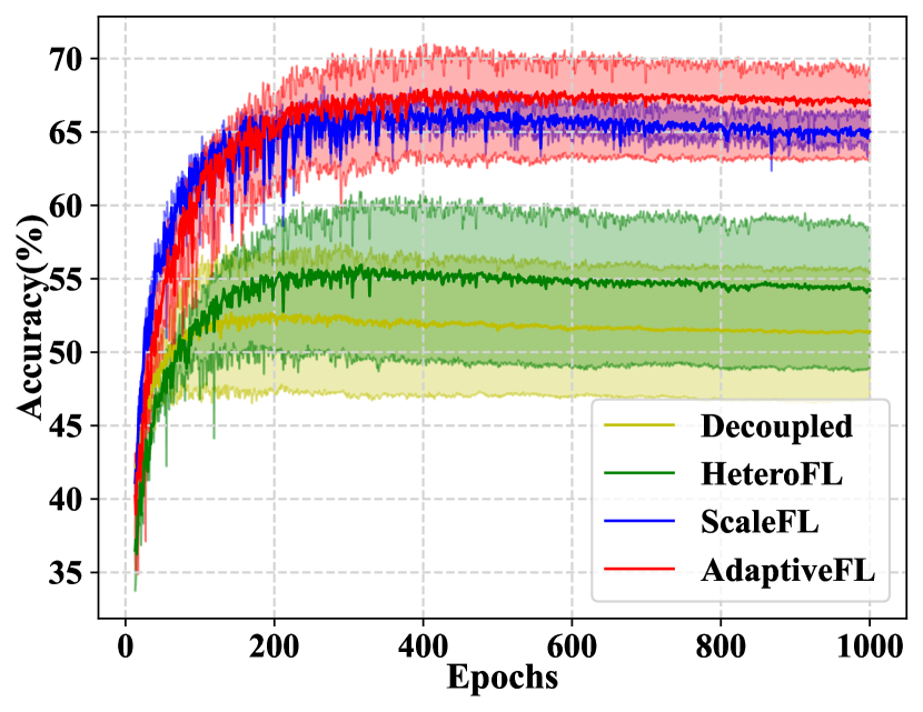
Submodel Performance. Figure 2 shows the learning trends of all methods on CIFAR-10/100 based on VGG16, where solid lines represent the “avg” accuracy of submodels. We can find that AdaptiveFL can achieve the best inference performance with the least variations for both non-IID and IID scenarios. For different heterogeneous FL methods, Figure 3 presents the shapes of VGG16 submodels together with their test accuracy information. We can find that AdaptiveFL consistently outperforms other heterogeneous FL methods under the premise of satisfying the resource constraints, which indicates the effectiveness of our fine-grained width-wise model pruning mechanism. Interestingly, we can find that 1.0 large models of HeteroFL and ScaleFL perform worse instead their 0.25 small counterparts. Conversely, as the model size increases, AdaptiveFL can achieve better results, indicating that it can smoothly transfer the knowledge learned by the submodels into large models.

4.3. Impacts of Different Configurations
Numbers of Participating Clients. To evaluate the scalability of AdaptiveFL, we conducted experiments considering different numbers of participating clients, i.e., = 50, 100, 200, and 500, respectively, on CIFAR-10 using ResNet18. Figure 4 compares AdaptiveFL with three baselines within a non-IID scenario (), where AdaptiveFL can always achieve the highest accuracy.


Proportions of Different Devices. Table 3 shows the performance of AdaptiveFL with different proportions (i.e., 8:1:1, 1:8:1, 1:1:8, and 4:3:3) of weak, medium, and strong devices on CIFAR-10. We can find that AdaptiveFL can achieve the best test accuracy in all cases. Note that as the proportion of strong devices increases, the global model performance of all FL methods improves.
| Algorithm | Proportion | |||||||
|---|---|---|---|---|---|---|---|---|
| 4:3:3 | 8:1:1 | 1:8:1 | 1:1:8 | |||||
| avg | full | avg | full | avg | full | avg | full | |
| All-Large | - | 79.76 | - | 79.76 | - | 79.76 | - | 79.76 |
| HeteroFL | 77.98 | 74.96 | 72.43 | 64.44 | 75.94 | 65.96 | 81.26 | 81.12 |
| ScaleFL | 79.94 | 78.12 | 75.89 | 72.03 | 78.40 | 72.30 | 82.55 | 82.81 |
| AdaptiveFL | 82.95 | 83.14 | 81.62 | 81.93 | 82.78 | 82.89 | 82.82 | 83.24 |
4.4. Ablation Study
Ablation of Fine-grained Pruning. To evaluate both fine- and coarse-grained pruning, we set to 3 and 1 for each level, respectively. Table 4 presents the ablation results of AdaptiveFL considering the effect of our fine-grained pruning method, showing that the fine-grained pruning method can achieve up to 9.38% inference accuracy improvements for AdaptiveFL. Note that the fine-grained methods can consistently achieve better inference results than their coarse-grained counterparts, since the fine-grained ones can better transfer the knowledge of small models to large models.
| Dataset | Model | Grained | Distribution | ||
|---|---|---|---|---|---|
| IID | = 0.6 | = 0.3 | |||
| CIFAR-10 | VGG16 | coarse | 80.1 | 78.9 | 74.27 |
| fine | 83.14 (+3.04) | 81.31 (+2.41) | 78.99 (+4.72) | ||
| ResNet18 | coarse | 72.43 | 71.92 | 66.07 | |
| fine | 77.2 (+4.77) | 74.89 (+2.97) | 70.97 (+4.9) | ||
| CIFAR-100 | VGG16 | coarse | 38.91 | 39.43 | 39.29 |
| fine | 40.93 (+2.02) | 38.88 (-0.55) | 41.17 (+1.88) | ||
| ResNet18 | coarse | 31.77 | 35.52 | 34.73 | |
| fine | 41.15 (+9.38) | 39.56 (+4.04) | 39.65 (+4.92) | ||
Ablation of RL-based Client Selection. To evaluate the effectiveness of our RL-based client selection strategy, we developed four variants of AdaptiveFL: i) “AdaptiveFL+Greedy” that always dispatches the largest model for each selected client; ii) “AdaptiveFL+Random” that selects clients for local training randomly; iii) “AdaptiveFL+C” that selects clients only based on curiosity reward; and iv) “AdaptiveFL+S” that selects clients only using resource rewards. Moreover, we use “AdaptiveFL+CS” to indicate the original AdaptiveFL implemented in Algorithm 1.


Figure 5 presents the ablation study results on CIFAR-100 with ResNet18 following IID distribution. To indicate the similarity between a sending model and its corresponding receiving model, we introduce a new metric called communication waste rate, defined as “”. The lower the rate, the closer the two models are, leading to less local pruning efforts. From Figure 5, we can find that our approach can achieve the highest accuracy with low communication waste (second only to RL-S).
4.5. Evaluation on Real Test-bed
Based on our real test-bed platform, we conducted experiments on a non-IID IoT dataset (i.e., Widar (fedaiot, )) with MobileNetV2 (mobilenetv2, ) models. We assumed that the FL-based AIoT system has 17 devices, each training round involves 10 selected devices, whose detail heterogeneous configurations are shown in Table 5.
| Type | Device | Comp | Mem | Num |
|---|---|---|---|---|
| Client-Weak | Raspberry Pi 4B | ARM Cortex-A72 CPU | 2G | 4 |
| Client-Medium | Jetson Nano | 128-core Maxwell GPU | 8G | 10 |
| Client-Strong | Jetson Xavier AGX | 512-core NVIDIA GPU | 32G | 3 |
| Server | Workstation | NVIDIA RTX 4090 GPU | 64G | 1 |
Figure 6 presents the AIoT devices used in our experiment and the comparison results obtained from our real test-bed platform. We can observe that AdaptiveFL achieves the best inference results even in real scenarios compared to all baselines.


5. Conclusion
This paper presented a novel Federated Learning (FL) approach named AdaptiveFL to enable effective knowledge sharing among heterogeneous devices for large-scale Artificial Intelligence of Things (AIoT) applications, considering the varying on-the-fly hardware resources of AIoT devices. Based on our proposed fine-grained width-wise model pruning mechanism, AdaptiveFL supports the generation of different local models, which will be selectively dispatched to their AIoT device counterparts in an adaptive manner according to their available local training resources. Experimental results show that our approach can achieve better inference performance than state-of-the-art heterogeneous FL methods.
Acknowledgment
This research is supported by the Natural Science Foundation of China (62272170), “Digital Silk Road” Shanghai International Joint Lab of Trustworthy Intelligent Software (22510750100), and the National Research Foundation Singapore and DSO National Laboratories under the AI Singapore Programme (AISG Award No: AISG2-RP-2020-019). Ming Hu and Mingsong Chen are the corresponding authors.
References
- [1] Brendan McMahan, Eider Moore, Daniel Ramage, Seth Hampson, and Blaise Agüera y Arcas. Communication-efficient learning of deep networks from decentralized data. In Proceedings of Artificial intelligence and statistics, pages 1273–1282, 2017.
- [2] Ming Hu, E Cao, Hongbing Huang, Min Zhang, Xiaohong Chen, and Mingsong Chen. Aiotml: A unified modeling language for aiot-based cyber-physical systems. IEEE Transactions on Computer-Aided Design of Integrated Circuits and Systems, 42(11):3545–3558, 2023.
- [3] Xinqian Zhang, Ming Hu, Jun Xia, Tongquan Wei, Mingsong Chen, and Shiyan Hu. Efficient federated learning for cloud-based aiot applications. IEEE Transactions on Computer-Aided Design of Integrated Circuits and Systems, 40(11):2211–2223, 2021.
- [4] Ming Hu, Zeke Xia, Dengke Yan, Zhihao Yue, Jun Xia, Yihao Huang, Yang Liu, and Mingsong Chen. Gitfl: Uncertainty-aware real-time asynchronous federated learning using version control. In IEEE Real-Time Systems Symposium (RTSS), pages 145–157, 2023.
- [5] Enmao Diao, Jie Ding, and Vahid Tarokh. Heterofl: Computation and communication efficient federated learning for heterogeneous clients. arXiv, 2020.
- [6] Minjae Kim, Sangyoon Yu, Suhyun Kim, and Soo-Mook Moon. Depthfl: Depthwise federated learning for heterogeneous clients. In Proceedings of International Conference on Learning Representations, 2022.
- [7] Fatih Ilhan, Gong Su, and Ling Liu. Scalefl: Resource-adaptive federated learning with heterogeneous clients. In Proceedings of the IEEE/CVF Conference on Computer Vision and Pattern Recognition, pages 24532–24541, 2023.
- [8] Yae Jee Cho, Andre Manoel, Gauri Joshi, Robert Sim, and Dimitrios Dimitriadis. Heterogeneous ensemble knowledge transfer for training large models in federated learning. In Proceedings of International Joint Conference on Artificial Intelligence, 2022.
- [9] Tao Lin, Lingjing Kong, Sebastian U Stich, and Martin Jaggi. Ensemble distillation for robust model fusion in federated learning. Advances in Neural Information Processing Systems, 33:2351–2363, 2020.
- [10] Ming Hu, Wenxue Duan, Min Zhang, Tongquan Wei, and Mingsong Chen. Quantitative timing analysis for cyber-physical systems using uncertainty-aware scenario-based specifications. IEEE Transactions on Computer-Aided Design of Integrated Circuits and Systems, 39(11):4006–4017, 2020.
- [11] Hao Li, Asim Kadav, Igor Durdanovic, Hanan Samet, and Hans Peter Graf. Pruning filters for efficient convnets. In Proceedings of ICLR, 2016.
- [12] Ming Hu, Jiepin Ding, Min Zhang, Frédéric Mallet, and Mingsong Chen. Enumeration and deduction driven co-synthesis of ccsl specifications using reinforcement learning. In 2021 IEEE Real-Time Systems Symposium (RTSS), pages 227–239, 2021.
- [13] Ming Hu, Min Zhang, Frédéric Mallet, Xin Fu, and Mingsong Chen. Accelerating reinforcement learning-based ccsl specification synthesis using curiosity-driven exploration. IEEE Transactions on Computers, 72(5):1431–1446, 2023.
- [14] Marc Bellemare, Sriram Srinivasan, Georg Ostrovski, Tom Schaul, David Saxton, and Remi Munos. Unifying count-based exploration and intrinsic motivation. Advances in neural information processing systems, 29, 2016.
- [15] Alex Krizhevsky, Geoffrey Hinton, et al. Learning multiple layers of features from tiny images. 2009.
- [16] Sebastian Caldas, Peter Wu, Tian Li, Jakub Konečný, H. Brendan McMahan, Virginia Smith, and Ameet Talwalkar. LEAF: A benchmark for federated settings. CoRR, abs/1812.01097, 2018.
- [17] Karen Simonyan and Andrew Zisserman. Very deep convolutional networks for large-scale image recognition. arXiv preprint arXiv:1409.1556, 2014.
- [18] Kaiming He, Xiangyu Zhang, Shaoqing Ren, and Jian Sun. Deep residual learning for image recognition. In Proceedings of the IEEE/CVF Conference on Computer Vision and Pattern Recognition, pages 770–778, 2016.
- [19] Samiul Alam, Tuo Zhang, Tiantian Feng, Hui Shen, Zhichao Cao, Dong Zhao, JeongGil Ko, Kiran Somasundaram, Shrikanth S Narayanan, Salman Avestimehr, et al. Fedaiot: A federated learning benchmark for artificial intelligence of things. arXiv, 2023.
- [20] Mark Sandler, Andrew Howard, Menglong Zhu, Andrey Zhmoginov, and Liang-Chieh Chen. Mobilenetv2: Inverted residuals and linear bottlenecks. In Proceedings of the IEEE/CVF Conference on Computer Vision and Pattern Recognition, pages 4510–4520, 2018.