This paper was converted on www.awesomepapers.org from LaTeX by an anonymous user.
Want to know more? Visit the Converter page.

Adaptive Temporal Difference Learning with
Linear Function Approximation

Tao Sun
College of Computer
National University of Defense Technology
Changsha, Hunan 410073, China
[email protected]
&Han Shen
Department of ECSE
Rensselaer Polytechnic Institute, Troy
Troy, NY, USA
[email protected]
&Tianyi Chen
Department of ECSE
Rensselaer Polytechnic Institute, Troy
Troy, NY, USA
[email protected]
&Dongsheng Li
College of Computer
University of California, Los Angeles
Changsha, Hunan 410073, China
[email protected]
   Tao Sun, Han Shen, Tianyi Chen, and Dongsheng Li The work of T. Sun and D. Li is sponsored in part by the National Key R&D Program of China under Grant (2018YFB0204300) and the National Natural Science Foundation of China under Grants (61932001 and 61906200). Tao Sun and Dongsheng Li are with the College of Computer, National University of Defense Technology, Changsha, 410073, Hunan, China (e-mails: [email protected], [email protected]). Han Shen and Tianyi Chen are with Department of ECSE, Rensselaer Polytechnic Institute, Troy, NY, USA, (e-mails: [email protected],[email protected]). The first and second authors contributed equally. Dongsheng Li is the corresponding author.
Abstract

This paper revisits the temporal difference (TD) learning algorithm for the policy evaluation tasks in reinforcement learning. Typically, the performance of TD(0) and TD(λ\lambda) is very sensitive to the choice of stepsizes. Oftentimes, TD(0) suffers from slow convergence. Motivated by the tight link between the TD(0) learning algorithm and the stochastic gradient methods, we develop a provably convergent adaptive projected variant of the TD(0) learning algorithm with linear function approximation that we term AdaTD(0). In contrast to the TD(0), AdaTD(0) is robust or less sensitive to the choice of stepsizes. Analytically, we establish that to reach an ϵ\epsilon accuracy, the number of iterations needed is O~(ϵ2ln41ϵ/ln41ρ)\tilde{O}(\epsilon^{-2}\ln^{4}\frac{1}{\epsilon}/\ln^{4}\frac{1}{\rho}) in the general case, where ρ\rho represents the speed of the underlying Markov chain converges to the stationary distribution. This implies that the iteration complexity of AdaTD(0) is no worse than that of TD(0) in the worst case. When the stochastic semi-gradients are sparse, we provide theoretical acceleration of AdaTD(0). Going beyond TD(0), we develop an adaptive variant of TD(λ\lambda), which is referred to as AdaTD(λ\lambda). Empirically, we evaluate the performance of AdaTD(0) and AdaTD(λ\lambda) on several standard reinforcement learning tasks, which demonstrate the effectiveness of our new approaches.

Index Terms:
Temporal Difference, Linear Function Approximation, Adaptive Step Size, MDP, Finite-Time Convergence

1 Introduction

Reinforcement learning (RL) involves a sequential decision-making procedure, where an agent takes (possibly randomized) actions in a stochastic environment over a sequence of time steps, and aims to maximize the long-term cumulative rewards received from the interacting environment. Owing to its generality, RL has been widely studied in many areas, such as control theory, game theory, operations research, multi-agent systems [1]. Temporal Difference (TD) learning is one of the most commonly used algorithms for policy evaluation in RL [2]. TD learning provides an iterative procedure to estimate the value function with respect to a given policy based on samples from a Markov chain. The classical TD algorithm adopts a tabular representation for the value function, which stores value estimates on a per state basis. In large-scale settings, the tabular-based TD learning algorithm can become intractable due to the increased number of states, and thus function approximation techniques are often combined with TD for better scalability and efficiency [3, 4].

The idea of TD learning with function approximation is essentially to parameterize the value function with a linear or nonlinear combination of fixed basis functions induced by the states that are termed feature vectors, and estimates the combination parameters in the same spirit of the tabular TD learning. Similar to all other parametric stochastic optimization algorithms, however, the performance of the TD learning algorithm with function approximation is very sensitive to the choice of stepsizes. Oftentimes, it suffers from slow convergence [5]. Ad-hoc adaptive modification of TD with function approximation has often been used empirically, but their convergence behavior and rate have not been fully understood. When implementing TD-learning, many practitioners use the adaptive optimizer but without theoretical guarantees. This paper is devoted to the development of a provably convergent adaptive algorithm to accelerate the TD(0) and TD(λ\lambda) algorithms. The key difficulty here is that the update used in the original TD does not follow the (stochastic) gradient direction of any objective function in an optimization problem, which prevents the use of the popular gradient-based optimization machinery. And the Markovian sampling protocol naturally involved in the TD update further complicates the analysis of adaptive and accelerated optimization algorithms.

1.1 Related works

We first briefly review related works in both the areas of TD learning and adaptive stochastic gradient.

Temporal difference learning. The great empirical success of TD [2] motivated active studies on the theoretical foundation of TD. The first convergence analysis of TD was given by [6] using stochastic approximation techniques. In [4], the characterization of limit points in TD with linear function approximation has been studied, giving new intuition about the dynamics of TD learning. The ODE-based method (e.g., [7]) has dramatically inspired the subsequent development of research on asymptotic convergence of TD. Early convergence results of TD learning were mostly asymptotic, e.g., [8], because the TD update does not follow the (stochastic) gradient direction of any fixed objective function. Non-asymptotic analysis for the gradient TD — a variant of the original TD has been first studied by [9], in which the authors reformulate the original problem as new primal-dual saddle point optimization. The finite-time analysis of TD with linear function approximation under i.i.d observation has been studied in [10]; in particular, it is assumed that observations in each iteration of TD are independently drawn from the steady-state distribution. In a concurrent line of research, TD has been considered in the view of the stochastic linear system, whose improved results are given by [11]. Even without any fixed objective function to optimize, the proofs of [10, 11] still follow a Lyapunov analysis like the SGD due to the i.i.d sampling assumption and quadratic functions structure. Nevertheless, a more realistic assumption for the data sampling in TD is the Markov rather than the i.i.d process. The finite-time convergence analysis under Markov sampling is first presented in [12], whose results are based on the controls of the gradient basis [Lemma 9, [12]] and a coupling [Lemma 11, [12]]. The finite-time analysis for stochastic linear system under the Markov sampling is established by [13, 14], which is a general formulate of TD and applies potentially to other problems. The finite-time analysis of multi-agent TD is proved by [15]. However, all the aforementioned work leverages the original TD update. In [16], the authors proposed an improvement of Q-learning, which can be used to TD, but with only asymptotic analysis being provided. An adaptive variant of two time-scale stochastic approximation was introduced by [17], that can also be applied to TD. In [18], the authors introduce the momentum techniques for reinforcement learning and an extension on DQN. In [19], the authors propose an adaptive scaling mechanism for TRPO and show that it is the “RL version” of traditional trust-region methods from convex analysis.

Adaptive stochastic gradient descent. In machine learning areas different but related to RL, adaptive stochastic gradient descent methods have been actively studied. The first adaptive gradient (AdaGrad) is proposed by [20, 21], and the algorithm demonstrated impressive numerical results when the gradients are sparse. While the original AdaGrad has a performance guarantee only in the convex case, the nonconvex AdaGrad has been studied by [22]. Besides the convex results, sharp analysis for nonconvex AdaGrad has also been investigated in [23]. Variants of AdaGrad have been developed in [24, 25], which use alternative updating schemes (the exponential moving average schemes) rather than the average of the square of the past iterate. The momentum technique applied to the adaptive stochastic algorithms gives birth to Adam and Nadam [26, 27]. However, in [28], the authors demonstrate that Adam may diverge under certain circumstances, and provide a new convergent Adam algorithm called AMSGrad. Another method given by [29] is the use of decreasing factors for moving the average of the square of the past iterates. In [30], the convergence for generic Adam-type algorithms has been studied, which contains various adaptive methods.

1.2 Comparison with existing analysis

Our analysis considers the Markov sampling setting and thus differs [10, 11]. It is worth mentioning that the stepsizes chosen in this paper are different from that of [17]: in [17], the “adaptive” means that the learning rate is reduced by multiplying a preset factor when transient error is dominated by the steady-state error; while in our paper, the “adaptive” inherits the notion from Ada training method, i.e., using the learning rate associated with the past gradients. Our analysis cannot directly follow the techniques given by [12, 13, 14, 16] since the learning rate in our algorithm is statistically dependent on past information, which breaks previous Lyapunov analysis.

Thus, this paper uses a delayed expectation technique rather than bounding a coupling [Lemma 11, [12]]. Furthermore, our analysis needs to deal with several terms related to adaptive style learning rates, which are quite complicated but absent in [12]. Since the adaptive learning rate consists of past iterates instead of being preset, these terms do not enjoy simple explicit bounds. To this end, in this paper, we develop novel techniques (Lemmas 3 and 7). On the other hand, our analysis is also different from the adaptive SGD because TD update is not the stochastic gradient of any objective function; it uses biased samples generated from the Markov chain.

1.3 Our contributions

Complementary to existing theoretical RL efforts, we propose the first provably convergent adaptive projected variant of the TD learning algorithm with linear function approximation that has finite-time convergence guarantees. For completeness of our analytical results, we investigate both the TD(0) algorithm as well as the TD(λ\lambda) algorithm. In a nutshell, our contributions are summarized in threefold:

c1) We develop the adaptive variants of the TD(0) and TD(λ\lambda) algorithms with linear function approximation. The new algorithms AdaTD(0) and AdaTD(λ\lambda) are simple to use.

c2) We establish the finite-time convergence guarantees of AdaTD(0) and AdaTD(λ\lambda), and they are not worse than those of TD and TD(λ\lambda) algorithms in the worst case.

c3) We test our AdaTD(0) and AdaTD(λ\lambda) on several standard RL benchmarks and show how these compare favorably to existing alternatives like TD(0), TD(λ\lambda), etc.

2 Preliminaries

This section introduces the notation, assumptions about the underlying MDP, and the setting of TD learning with linear function approximation.

Notation: The coordinate jj of a vector 𝐱{\bf x} is denoted by 𝐱j{\bf x}_{j} and 𝐱{\bf x}^{\top} is transpose of 𝐱{\bf x}. We use 𝔼[]\mathbb{E}[\cdot] to denote the expectation with respect to the underlying probability space, and \|\cdot\| for 2\ell_{2} norm. Given a constant R>0R>0 and 𝐲d{\bf y}\in\mathbb{R}^{d}, ProjR(𝐲)\textbf{Proj}_{R}({\bf y}) denotes the projection of 𝐲{\bf y} to the ball {𝐱d𝐱R}\{{\bf x}\in\mathbb{R}^{d}\mid\|{\bf x}\|\leq R\}. For a matrix AS×dA\in\mathbb{R}^{S\times d}, ProjA(𝐲)\textbf{Proj}_{A}({\bf y}) denotes the projection to space {A𝐱𝐱d}\{A{\bf x}\mid{\bf x}\in\mathbb{R}^{d}\}. We denote the sub-algebra as σk:=σ(𝜽0,𝜽1,,𝜽k)\sigma^{k}:=\sigma({\bm{\theta}}^{0},{\bm{\theta}}^{1},\ldots,{\bm{\theta}}^{k}), where 𝜽k{\bm{\theta}}^{k} is the kkth iterate. We use O~(b)\tilde{O}(b) and Θ~(b)\tilde{\Theta}(b) to hide the logarithmic factor of bb.

2.1 Markov Decision Process

Consider a Markov decision process (MDP) described as a tuple (𝒮,𝒜,𝒫,,γ(\mathcal{S},\mathcal{A},\mathcal{P},\mathcal{R},\gamma), where 𝒮\mathcal{S} denotes the state space, 𝒜\mathcal{A} denotes the action space, 𝒫\mathcal{P} represents the transition matrix, \mathcal{R} is the reward function, and 0<γ<10<\gamma<1 is the discount factor. In this case, let 𝒫(s|s)\mathcal{P}(s^{\prime}|s) denote the transition probability from state ss to state ss^{\prime}. The corresponding transition reward is (s,s)\mathcal{R}(s,s^{\prime}). We consider the finite-state case, i.e., 𝒮\mathcal{S} consists of |𝒮||\mathcal{S}| elements, and a stochastic policy μ:𝒮𝒜\mu:{\cal S}\rightarrow{\cal A} that specifies an action given the current state ss. We use the following two assumptions on the stationary distribution and the reward.

Assumption 1

The transition rewards are uniformly bounded, i.e.,

|(s,s)|B,s,s𝒮.|\mathcal{R}(s,s^{\prime})|\leq B,~{}\forall\,\,s,s^{\prime}\in\mathcal{S}.
Assumption 2

For any two states s,s𝒮s,s^{\prime}\in\mathcal{S}, it holds that

π(s)=limt𝒫(st=s|s0=s)>0.\pi(s^{\prime})=\lim_{t\to\infty}\mathcal{P}(s_{t}=s^{\prime}|s_{0}=s)>0.

There exist κ¯>0\bar{\kappa}>0 and 0ρ<10\leq\rho<1 such that

sups𝒮{s𝒮|𝒫(st=ss0=s)π(s)|}κ¯ρt.\sup_{s\in\mathcal{S}}\{\sum_{s^{\prime}\in\mathcal{S}}|\mathcal{P}(s_{t}=s^{\prime}\mid s_{0}=s)-\pi(s^{\prime})|\}\leq\bar{\kappa}\rho^{t}.

Assumptions 1 and 2 are standard in MDP. For irreducible and aperiodic Markov chains, Assumption 2 can always hold [31]. The constant ρ\rho represents the Markov chain’s speed accessing the stationary distribution π\pi. When the number of states is finite, the Markovian transition kernel is a matrix 𝒫\mathcal{P}, and ρ\rho is identical to the second largest eigenvalue of 𝒫\mathcal{P}. An important notion in the Markov chain is the mixing time, which measures the time that a Markov chain needs for its current state distribution roughly matches the stationary one π\pi. Given an ϵ>0\epsilon>0, the mixing time is defined as

τ(ϵ):=mint+{κ¯ρtϵ}.\tau(\epsilon):=\min_{t\in\mathbb{Z}^{+}}\{\bar{\kappa}\rho^{t}\leq\epsilon\}.

With Assumption 2, we can see τ(ϵ)=O(ln1ϵ/ln1ρ)\tau(\epsilon)=O({\ln\frac{1}{\epsilon}}/{\ln\frac{1}{\rho}}). That means if ρ\rho is small, the mixing time is short.

This paper considers the on policy setting, where both the target and behavior policies are μ\mu. For a given policy μ\mu, since the actions or the distribution of actions will be uniquely determined, we thus eliminate the dependence on the action in the rest of the paper. We denote the expected reward at a given state ss by

(s):=s𝒮𝒫(s|s)(s,s).\mathcal{R}(s):=\sum_{s^{\prime}\in\mathcal{S}}\mathcal{P}(s^{\prime}|s)\mathcal{R}(s,s^{\prime}).

The value function Vμ:𝒮V_{\mu}:\mathcal{S}\to\mathbb{R} associated with a policy μ\mu is the expected cumulative discounted reward from a given state ss, that is

Vμ(s)=𝔼[t=0γt(st)|s0=s],V_{\mu}(s)=\mathbb{E}\left[\sum_{t=0}^{\infty}\gamma^{t}\mathcal{R}(s_{t}){\,\Big{|}\,}s_{0}=s\right],

where the expectation is taken over the trajectory of states generated under 𝒫\mathcal{P} and μ\mu. The restriction on discount 0<γ<10<\gamma<1 can guarantee the boundedness of Vμ(s)V_{\mu}(s). The Markovian property of MDP yields the well-known Bellman equation

𝒯μVμ=Vμ,\mathcal{T}_{\mu}V_{\mu}=V_{\mu}, (1)

where the operator 𝒯μ\mathcal{T}_{\mu} on VV is defined as

(𝒯μV)(s):=(s)+γs𝒮𝒫(s|s)V(s),s𝒮.(\mathcal{T}_{\mu}V)(s):=\mathcal{R}(s)+\gamma\sum_{s^{\prime}\in\mathcal{S}}\mathcal{P}(s^{\prime}|s)V(s^{\prime}),\,\,s\in\mathcal{S}.

Solving the (linear) Bellman equation allows us to find the value function VμV_{\mu} induced by a given policy μ\mu. However, in practice, |𝒮||\mathcal{S}| is usually very large and computationally intractable. An alternative method is to leverage the linear [1] or non-linear function approximations (e.g., kernels and neural networks [32]). We focus on the linear case here, that is

Vμ(s)V𝜽(s):=ϕ(s)𝜽,V_{\mu}(s)\approx V_{{\bm{\theta}}}(s):=\phi(s)^{\top}{\bm{\theta}}, (2)

where ϕ(s)d\phi(s)\in\mathbb{R}^{d} is the feature vector for state ss, and 𝜽d{\bm{\theta}}\in\mathbb{R}^{d} is a parameter vector. To reduce difficulty caused by the dimension, dd is set smaller than |𝒮||\mathcal{S}|. With the linear function approximator, the vector V𝜽|𝒮|V_{{\bm{\theta}}}\in\mathbb{R}^{|\mathcal{S}|} becomes

V𝜽=Φ𝜽,\displaystyle V_{{\bm{\theta}}}=\Phi{\bm{\theta}},

where the feature matrix is defined as

Φ:=[ϕ(s1),ϕ(s2),,ϕ(s|𝒮|)]|𝒮|×d\Phi:=[\phi(s_{1}),\phi(s_{2}),\ldots,\phi(s_{|\mathcal{S}|})]^{\top}\in\mathbb{R}^{{|\mathcal{S}|}\times d}

with sns_{n} being the nnth state.

Assumption 3

For any state s𝒮s\in\mathcal{S}, we assume the feature vector is uniformly bounded such that ϕ(s)1\|\phi(s)\|\leq 1, and the feature matrix Φ\Phi is full column-rank.

It is not hard to guarantee Assumption 3 since the feature map ϕ\phi is chosen by the users and |𝒮|>d|\mathcal{S}|>d. With Assumptions 2 and 3, we can see that the matrix ΦDiag(π)Φ\Phi^{\top}\textrm{Diag}(\pi)\Phi is positive define, and we denote its minimal eigenvalue as follows

ω:=λmin(ΦDiag(π)Φ)>0.\omega:=\lambda_{\min}\left(\Phi^{\top}\textrm{Diag}(\pi)\Phi\right)>0.

With the linear approximation of value function, the task then is tantamount to finding 𝜽d{\bm{\theta}}\in\mathbb{R}^{d} that obeys the Bellman equation given by

Φ𝜽=𝒯μΦ𝜽.\Phi{\bm{\theta}}=\mathcal{T}_{\mu}\Phi{\bm{\theta}}.

However, 𝜽{\bm{\theta}} that satisfies such an equation may not exist if Vμ{Φ𝜽𝜽d}V_{\mu}\notin\{\Phi{\bm{\theta}}\mid{\bm{\theta}}\in\mathbb{R}^{d}\}. Instead, there always exists a unique solution 𝜽{\bm{\theta}}^{*} for the projected Bellman equation [4], given by

Φ𝜽=ProjΦ(𝒯μΦ𝜽),\Phi{\bm{\theta}}^{*}=\textbf{Proj}_{\Phi}(\mathcal{T}_{\mu}\Phi{\bm{\theta}}^{*}), (3)

where ProjΦ\textbf{Proj}_{\Phi} is the projection onto the span of Φ\Phi’s columns.

3 Adaptive Temporal Difference Learning

3.1 TD with linear function approximation

TD(0) algorithm starts with an initial parameter θ0\theta^{0}. At iteration kk, after sampling states sks_{k}, sk+1s_{k+1}, and reward r(sk+1,sk)r(s_{k+1},s_{k}) from a Markov chain, we can compute the TD (temporal difference) error which is also called the Bellman error:

dk:=r(sk+1,sk)+γV𝜽(sk+1)V𝜽(sk).d_{k}:=r(s_{k+1},s_{k})+\gamma V_{{\bm{\theta}}}(s_{k+1})-V_{{\bm{\theta}}}(s_{k}). (4)

The TD error is subsequently used to compute the stochastic semi-gradient:

𝐠¯(𝜽k;sk,sk+1):=dkV𝜽k(sk)=dkϕ(sk).\overline{{\bf g}}({\bm{\theta}}^{k};s_{k},s_{k+1}):=d_{k}\nabla V_{{\bm{\theta}}^{k}}(s_{k})=d_{k}\phi(s_{k}). (5)

The traditional TD(0) with linear function approximation performs SGD-like update as

𝜽k+1=𝜽k+η𝐠¯(𝜽k;sk,sk+1).{\bm{\theta}}^{k+1}={\bm{\theta}}^{k}+\eta\overline{{\bf g}}({\bm{\theta}}^{k};s_{k},s_{k+1}). (6)
Algorithm 1 Projected TD(0) Learning
1:Parameters: learning rate η\eta.
2:Initialization: 𝐠0=0{\bf g}^{0}=\textbf{0}, 𝐦0=0{\bf m}^{0}=\textbf{0}, v0=0v^{0}=0
3:for k=1,2,k=1,2,\ldots do
4:     sample a state transition sksk+1s_{k}\rightarrow s_{k+1} from μ\mu
5:     calculate 𝐠¯(𝜽k;sk,sk+1)\overline{{\bf g}}({\bm{\theta}}^{k};s_{k},s_{k+1}) in (5)
6:     update the parameter 𝜽k{\bm{\theta}}^{k} as
𝜽k+1=ProjR[𝜽k+η𝐠¯(𝜽k;sk,sk+1)],{\bm{\theta}}^{k+1}=\textbf{Proj}_{R}[{\bm{\theta}}^{k}+\eta\overline{{\bf g}}({\bm{\theta}}^{k};s_{k},s_{k+1})], (7)
7:end for

The update TD(0) makes sense because the direction 𝐠¯(𝜽;sk,sk+1)\overline{{\bf g}}({\bm{\theta}};s_{k},s_{k+1}) is a good one since it is asymptotically close to the direction whose limit point is 𝜽{\bm{\theta}}^{*}. Specifically, it has been established that [4]

limk𝔼[𝐠¯(𝜽;sk,sk+1)]=𝐠(𝜽),\lim_{k\rightarrow\infty}\mathbb{E}[\overline{{\bf g}}({\bm{\theta}};s_{k},s_{k+1})]={\bf g}({\bm{\theta}}),

where 𝐠(𝜽){\bf g}({\bm{\theta}}) is defined as

𝐠(𝜽):=ΦDiag(π)(𝒯μΦ𝜽Φ𝜽).{\bf g}({\bm{\theta}}):=\Phi^{\top}\textrm{Diag}(\pi)(\mathcal{T}_{\mu}\Phi{\bm{\theta}}-\Phi{\bm{\theta}}).

We term 𝐠(𝜽){\bf g}({\bm{\theta}}) as the limiting update direction, ensuring that 𝐠(𝜽)=0{\bf g}({\bm{\theta}}^{*})=\textbf{0}. Note that while 𝐠¯(𝜽;sk,sk+1)\overline{{\bf g}}({\bm{\theta}};s_{k},s_{k+1}) is an unbiased estimate under the stationary π\pi, it is not for a finite kk due to the Markovian property of sks_{k}. Therefore, the TD(0) update (6) is asymptotically akin to the stochastic approximation

𝜽k+1=𝜽k+η𝐠¯(𝜽k;s,s),{\bm{\theta}}^{k+1}={\bm{\theta}}^{k}+\eta\overline{{\bf g}}({\bm{\theta}}^{k};s,s^{\prime}),

where s,ss,s^{\prime} are independently drawn from the stationary distribution π\pi.

Nevertheless, an important property of the limiting direction 𝐠(𝜽){\bf g}({\bm{\theta}}), found by [4], is that: for any 𝜽d{\bm{\theta}}\in\mathbb{R}^{d}, we have

𝜽𝜽,𝐠(𝜽)(1γ)ω𝜽𝜽2.\langle{\bm{\theta}}^{*}-{\bm{\theta}},{\bf g}({\bm{\theta}})\rangle\geq(1-\gamma)\omega\|{\bm{\theta}}^{*}-{\bm{\theta}}\|^{2}. (8)

An important observation follows from this inequality readily: only one 𝜽{\bm{\theta}}^{*} satisfies 𝐠(𝜽)=0{\bf g}({\bm{\theta}}^{*})=\textbf{0}. We can show this by contradiction. If there exists another 𝜽¯\bar{{\bm{\theta}}} such that 𝐠(𝜽¯)=0{\bf g}(\bar{{\bm{\theta}}})=\textbf{0}, we have 0=𝜽𝜽¯,𝐠(𝜽¯)(1γ)ω𝜽𝜽¯20=\langle{\bm{\theta}}^{*}-\bar{{\bm{\theta}}},{\bf g}(\bar{{\bm{\theta}}})\rangle\geq(1-\gamma)\omega\|{\bm{\theta}}^{*}-\bar{{\bm{\theta}}}\|^{2}, which again means 𝜽=𝜽¯{\bm{\theta}}^{*}=\bar{{\bm{\theta}}}.

To ensure the boundedness of 𝜽k{\bm{\theta}}^{k} and simplify the convergence analysis, projection is used in (7) (see e.g., [12]). In [12], it has been shown that if R2B/ω(1γ)32R\geq 2B/\sqrt{\omega}(1-\gamma)^{\frac{3}{2}} (BB has appeared in Assumption 1), the projected TD(0) does not exclude all the limit points of the TD(0) (such a fact still holds for our proposed algorithms). The finite-time convergence of projected TD(0) is analyzed by [12]. The projection step is removed in [13], with almost the same results being proved. But in [13], the authors just studied the constant stepsize, while [12] shows more cases, including diminishing stepsize cases. In this paper, we consider a more complicated scheme that cannot be analyzed using techniques in [13]. Thus, the projection is still needed.

3.2 Adaptive TD development

Motivated by the recent success of adaptive SGD methods such as [20, 24, 28], this paper aims to develop an adaptive version of TD with linear function approximation that we term AdaTD(0) (adaptive TD). Unlike TD(0) method, in which step size is often a constant, AdaTD(0) seeks to scale the step size depending on the norm of stochastic gradient. Additionally, instead of using a one-step gradient, AdaTD(0) utilizes momentum, which gives the algorithm a memory of history information.

As presented in the last section, 𝐠¯(𝜽;sk,sk+1)\overline{{\bf g}}({\bm{\theta}};s_{k},s_{k+1}) is a stochastic estimate of 𝐠(𝜽){\bf g}({\bm{\theta}}). Based on this observation, we develop the adaptive scheme for TD(0). Different from projected TD(0), we use the update direction 𝐦k{\bf m}^{k}, which is the exponentially weighted average of stochastic gradients. It is further scaled by vkv^{k}, the moving average of the squared norm of stochastic semi-gradients. Intuitively, when the gradient is large, the algorithm will take smaller steps. To prevent a too large scaling, we use a positive hyper-parameter δ\delta for numerical stability. The AdaTD(0) update is given by (9). The key difference between AdaTD(0) and the TD(0) method is that AdaTD(0) utilizes the history information in the update of both first moment estimate 𝐦k{\bf m}^{k} and second moment estimate vkv^{k}. Unlike projected TD(0) whose asymptotically expected TD update, 𝐠(𝜽k){\bf g}({\bm{\theta}}^{k}), is a good direction as is evident from (8), the update direction 𝐦k{\bf m}^{k} in AdaTD(0) is an exponentially weighted version of 𝐠¯(𝜽k;sk,sk+1)\overline{{\bf g}}({\bm{\theta}}^{k};s_{k},s_{k+1}), which makes our analysis more challenging.

Although the variance term in AdaTD(0) is used as a sum form, it can be rewritten as an exponentially weighted moving average. If we denote v^k:=i=1k𝐠i2k=vkk\hat{v}^{k}:=\frac{\sum_{i=1}^{k}\|{\bf g}^{i}\|^{2}}{k}=\frac{v^{k}}{k}, the last two steps of Ada-TD(0) can be reformulated as

v^k\displaystyle\hat{v}^{k} =(11k)v^k1+1kv^k,\displaystyle=(1-\frac{1}{k})\hat{v}^{k-1}+\frac{1}{k}\hat{v}^{k},
𝜽k+1\displaystyle{\bm{\theta}}^{k+1} =ProjR(𝜽k+ηk𝐦k/(v^k+δk)1/2),\displaystyle=\textbf{Proj}_{R}({\bm{\theta}}^{k}+\frac{\eta}{\sqrt{k}}{\bf m}^{k}/(\hat{v}^{k}+\frac{\delta}{k})^{1/2}),

Note that in this form, weights are {1/k}k1\{1/k\}_{k\geq 1} and stepsizes are {ηk}k1\{\frac{\eta}{\sqrt{k}}\}_{k\geq 1}, which obey the sufficient conditions to guarantee the convergence of Adam-type algorithms with exponentially weighted average variance term [29, 30].

Algorithm 2 Projected Adaptive TD(0) Learning 1:Parameters: η,δ\eta,\delta, β\beta, γ\gamma, RR. 2:Initialization: 𝐠0=0{\bf g}^{0}=\textbf{0}, 𝐦0=0{\bf m}^{0}=\textbf{0}, v0=0v^{0}=0 3:for k=1,2,k=1,2,\ldots do 4:     sample a state transition sksk+1s_{k}\rightarrow s_{k+1} from μ\mu 5:     calculate 𝐠¯(𝜽k;sk,sk+1)\overline{{\bf g}}({\bm{\theta}}^{k};s_{k},s_{k+1}) in (5) 6:     update the parameter 𝜽k{\bm{\theta}}^{k} as 𝐦k\displaystyle{\bf m}^{k} =β𝐦k1+(1β)𝐠¯(𝜽k;sk,sk+1),\displaystyle=\beta{\bf m}^{k-1}+(1-\beta)\overline{{\bf g}}({\bm{\theta}}^{k};s_{k},s_{k+1}), (9a) vk\displaystyle v^{k} =vk1+𝐠¯(𝜽k;sk,sk+1)2,\displaystyle=v^{k-1}+\|\overline{{\bf g}}({\bm{\theta}}^{k};s_{k},s_{k+1})\|^{2}, (9b) 𝜽k+1\displaystyle{\bm{\theta}}^{k+1} =ProjR(𝜽k+η𝐦k/vk+δ).\displaystyle=\textbf{Proj}_{R}({\bm{\theta}}^{k}+\eta{\bf m}^{k}/\sqrt{v^{k}+\delta}). (9c) 7:end for Algorithm 3 Projected Adaptive TD(λ\lambda) Learning 1:parameters: η\eta, β\beta, γ\gamma, δ\delta, λ\lambda, R^\hat{R}. 2:initialization: 𝐠0=0{\bf g}^{0}=\textbf{0}, 𝐳0=0{\bf z}^{0}=\textbf{0}, 𝐦0=0{\bf m}^{0}=\textbf{0}, v0=0v^{0}=0 3:for k=1,2,k=1,2,\ldots do 4:     sample a state transition sksk+1s_{k}\rightarrow s_{k+1} from μ\mu 5:     update 𝐳k=(γλ)𝐳k1+ϕ(sk){\bf z}^{k}=(\gamma\lambda){\bf z}^{k-1}+\phi(s_{k}) 6:     update 𝐠¯λ(𝜽;sk,sk+1,𝐳k):=r(sk+1,sk)𝐳k\displaystyle\overline{{\bf g}}^{\lambda}({\bm{\theta}};s_{k},s_{k+1},{\bf z}^{k}):=r(s_{k+1},s_{k}){\bf z}^{k} +γϕ(sk+1)𝜽𝐳kϕ(sk)𝜽𝐳kd,\displaystyle\qquad+\gamma\phi(s_{k+1})^{\top}{\bm{\theta}}{\bf z}^{k}-\phi(s_{k})^{\top}{\bm{\theta}}{\bf z}^{k}\in\mathbb{R}^{d}, (10) 7:     update the parameter 𝜽k{\bm{\theta}}^{k} as (9) with RR^R\leftarrow\hat{R} 8:end for

3.3 Finite-time analysis of projected AdaTD(0)

Because the main results depend on constants related to the bounds, we present them in Lemma 1.

Lemma 1

The following bounds hold for (𝛉k)k0({\bm{\theta}}^{k})_{k\geq 0} generated by AdaTD(0)

𝜽k𝜽2R,𝐠kG,𝐦kG\displaystyle\|{\bm{\theta}}^{k}-{\bm{\theta}}^{*}\|\leq 2R,~{}~{}~{}\|{\bf g}^{k}\|\leq G,~{}~{}~{}\|{\bf m}^{k}\|\leq G (11)

where we define 𝐠k:=𝐠¯(𝛉k;sk,sk+1){\bf g}^{k}:=\overline{{\bf g}}({\bm{\theta}}^{k};s_{k},s_{k+1}), and G:=2R+BG:=2R+B.

Lemma 1 follows readily. The bounds presented in Lemma 1 are critical for the subsequent analysis.

The convergence analysis of AdaTD(0) is more challenging than that of both TD and adaptive SGD. Compared with the analysis of adaptive SGD methods in e.g., [20, 24, 28], even under the i.i.d. sampling, the stochastic direction 𝐠¯(𝜽k;sk,sk+1)\overline{{\bf g}}({\bm{\theta}}^{k};s_{k},s_{k+1}) used in (9) fails to be the stochastic gradient of any objective function, aside from the fact that samples are drawn from a Markov chain. Compared with TD(0), the actual update of 𝜽k{\bm{\theta}}^{k} in AdaTD(0) involves the history information of both the first and the second moments of 𝐠¯(𝜽k;sk,sk+1)\overline{{\bf g}}({\bm{\theta}}^{k};s_{k},s_{k+1}), which makes the analysis of TD in e.g., [12, 13] intractable.

Theorem 1

Suppose (𝛉k)k0({\bm{\theta}}^{k})_{k\geq 0} are generated by AdaTD(0) with R2B/ω(1γ)32R\geq 2B/\sqrt{\omega}(1-\gamma)^{\frac{3}{2}} under the Markovian observation. Given η>0,δ>0,0β<1\eta>0,\delta>0,0\leq\beta<1, we have

min1kK𝔼(𝜽𝜽k2)\displaystyle\min_{1\leq k\leq K}\mathbb{E}(\|{\bm{\theta}}^{*}-{\bm{\theta}}^{k}\|^{2})
[C1ln(δ+KG2δ)]/K+C2/K,\displaystyle\qquad\leq\Big{[}C_{1}\ln\big{(}\frac{\delta+KG^{2}}{\delta}\big{)}\Big{]}/\sqrt{K}+C_{2}/\sqrt{K},

where C1C_{1} and C2C_{2} are given as

C1\displaystyle C_{1} :=16(lnK/ln1ρ)2Gδ(1γ)2ω2+2ηβG(1β)(1γ)ω\displaystyle:=\frac{16(\ln K/\ln\frac{1}{\rho})^{2}G}{\sqrt{\delta}(1-\gamma)^{2}\omega^{2}}+\frac{2\eta\beta G}{(1-\beta)(1-\gamma)\omega}
+ηG(1γ)ω+4RG2(1γ)ωδ=O((lnK/ln1ρ)2δ),\displaystyle\quad+\frac{\eta G}{(1-\gamma)\omega}+\frac{4RG^{2}}{(1-\gamma)\omega\delta}=O(\frac{(\ln K/\ln\frac{1}{\rho})^{2}}{\sqrt{\delta}}),
C2\displaystyle C_{2} :=4R2G(1γ)ωη+4RηG2δ12(1β)(1γ)ω\displaystyle:=\frac{4R^{2}G}{(1-\gamma)\omega\eta}+\frac{4R\eta G^{2}}{\delta^{\frac{1}{2}}(1-\beta)(1-\gamma)\omega}
+4Rκ¯(B+Rγ+R)Gδ(1γ)ω=O(1δ).\displaystyle\quad+\frac{4R\bar{\kappa}(B+R\gamma+R)G}{\sqrt{\delta}(1-\gamma)\omega}=O(\frac{1}{\sqrt{\delta}}).

With Theorem 1, to achieve ϵ\epsilon-accuracy for min1kK{𝔼(𝜽𝜽k2)}\min_{1\leq k\leq K}\{\mathbb{E}(\|{\bm{\theta}}^{*}-{\bm{\theta}}^{k}\|^{2})\}, we need

C2/Kϵ/2,C1ln(δ+KG2δ)Kϵ/2.\displaystyle C_{2}/\sqrt{K}\leq\epsilon/2,~{}~{}~{}~{}~{}~{}\frac{C_{1}\ln\big{(}\frac{\delta+KG^{2}}{\delta}\big{)}}{\sqrt{K}}\leq\epsilon/2. (12)

Since C2=O(1)C_{2}=O(1), with the first inequality of (12), K=O~(1ϵ2)K=\tilde{O}(\frac{1}{\epsilon^{2}}). Further, due to C1=O([lnK/ln1ρ]2)=O([ln1ϵ/ln1ρ]2)C_{1}=O([\ln K/\ln\frac{1}{\rho}]^{2})=O([\ln\frac{1}{\epsilon}/\ln\frac{1}{\rho}]^{2}), with the second inequality of (12), we have C1lnK/K=O~(C1/K)=O(ϵ)C_{1}\ln K/\sqrt{K}=\tilde{O}(C_{1}/\sqrt{K})=O(\epsilon). Therefore, we obtain a solution whose square distance to 𝜽{\bm{\theta}}^{*} is ϵ\epsilon, the iteration needed is

O~(C12/ϵ2)=O~(ln41ϵ/(ϵ2ln41ρ)).\displaystyle\tilde{O}\left(C_{1}^{2}/\epsilon^{2}\right)=\tilde{O}\left(\ln^{4}\frac{1}{\epsilon}\Big{/}(\epsilon^{2}\ln^{4}\frac{1}{\rho})\right). (13)

When ρ\rho is much smaller than 11, the term ln1ϵ/ln1ρ\ln\frac{1}{\epsilon}/\ln\frac{1}{\rho} keeps at a relatively small level. Recall that the state-of-the-art convergence result of TD(0) given in [12] is O~(ln21ϵ/(ϵ2ln21ρ))\tilde{O}(\ln^{2}\frac{1}{\epsilon}\big{/}(\epsilon^{2}\ln^{2}\frac{1}{\rho})), the rate of AdaTD(0) is close to TD(0) in the general case. We do not present a faster speed for technical reasons. In fact, this is also the case for the adaptive SGD [20, 24, 28]. Specifically, although numerical results demonstrate the advantage of adaptive methods, the worst-case convergence rate of adaptive methods is still similar to that of the stochastic gradient descent method. To reach a desired error as min1kK{𝔼(f(𝐱k)2)}ϵ\min_{1\leq k\leq K}\{\mathbb{E}(\|\nabla f({\bf x}^{k})\|^{2})\}\leq\epsilon in adaptive SGD, where 𝐱k{\bf x}^{k} is the kkth iterative and ϵ>0\epsilon>0, the iteration number KK needs to be set as O(1ϵ2)O(\frac{1}{\epsilon^{2}}), which is identical to the SGD.

Sketch of the proofs: Now, we present the sketch of the proofs for the main result. Because AdaTD(0) does not have any objective function to optimize, we consider sequence the (𝜽k𝜽2)k0(\|{\bm{\theta}}^{k}-{\bm{\theta}}^{*}\|^{2})_{k\geq 0}.

Using the update (9), we have

𝜽𝜽k+12𝜽𝜽k2\displaystyle\|{\bm{\theta}}^{*}-{\bm{\theta}}^{k+1}\|^{2}-\|{\bm{\theta}}^{*}-{\bm{\theta}}^{k}\|^{2}
2η𝐦k,𝜽k𝜽(vk+δ)12+η2𝐦k2(vk+δ)\displaystyle\leq\frac{2\eta\langle{\bf m}^{k},{\bm{\theta}}^{k}-{\bm{\theta}}^{*}\rangle}{(v^{k}+\delta)^{\frac{1}{2}}}+\frac{\eta^{2}\|{\bf m}^{k}\|^{2}}{(v^{k}+\delta)}
2η𝜽k𝜽,𝐦k/(vk1+δ)12I1k+η2𝐦k2/(vk+δ)I2k\displaystyle\leq\underbrace{2\eta\langle{\bm{\theta}}^{k}-{\bm{\theta}}^{*},{\bf m}^{k}\rangle/(v^{k-1}+\delta)^{\frac{1}{2}}}_{I_{1}^{k}}+\underbrace{\eta^{2}\|{\bf m}^{k}\|^{2}/(v^{k}+\delta)}_{I_{2}^{k}}
+2η𝜽k𝜽,𝐦k(1/(vk+δ)121/(vk1+δ)12)I3k.\displaystyle\quad+\underbrace{2\eta\langle{\bm{\theta}}^{k}-{\bm{\theta}}^{*},{\bf m}^{k}\rangle(1/(v^{k}+\delta)^{\frac{1}{2}}-1/(v^{k-1}+\delta)^{\frac{1}{2}})}_{I_{3}^{k}}. (14)

Here, we split the term 𝐦k,𝜽k𝜽/(vk+δ)12\langle{\bf m}^{k},{\bm{\theta}}^{k}-{\bm{\theta}}^{*}\rangle/(v^{k}+\delta)^{\frac{1}{2}} as I1k+I3kI_{1}^{k}+I_{3}^{k} because both 𝐦k{\bf m}^{k} and vkv^{k} statistically depends on 𝐠¯(𝜽k;sk,sk+1)\overline{{\bf g}}({\bm{\theta}}^{k};s_{k},s_{k+1}), which makes it hard to calculate the expectation. Subtracting I1k-I_{1}^{k} to both sides of (3.3), we get

I1k𝜽𝜽k2𝜽𝜽k+12+I2k+I3k.\displaystyle-I_{1}^{k}\leq\|{\bm{\theta}}^{*}-{\bm{\theta}}^{k}\|^{2}-\|{\bm{\theta}}^{*}-{\bm{\theta}}^{k+1}\|^{2}+I_{2}^{k}+I_{3}^{k}. (15)

With division (15), the analysis can be divided into three parts: A) determine the lower bound of 𝔼[I1k]-\mathbb{E}[I_{1}^{k}] (i.e, the upper bound of 𝔼[I1k]\mathbb{E}[I_{1}^{k}]); B) prove the summability of (𝔼[I2k])k1(\mathbb{E}[I_{2}^{k}])_{k\geq 1}, i.e., k=1+I2k<+\sum_{k=1}^{+\infty}I_{2}^{k}<+\infty; C) prove the summability of (𝔼[I3k])k1(\mathbb{E}[I_{3}^{k}])_{k\geq 1}.

A) Calculating the upper bound of 𝔼[I1k]\mathbb{E}{[I_{1}^{k}]} is the most difficult part, which consists of two substeps. Since 𝐦k{\bf m}^{k} is a convex combination of 𝐦k1{\bf m}^{k-1} and 𝐠¯(𝜽k;sk,sk+1)\overline{{\bf g}}({\bm{\theta}}^{k};s_{k},s_{k+1}). We recursively bound 𝔼[I1k]\mathbb{E}[I_{1}^{k}] by analyzing 𝔼[𝜽k𝜽,𝐠¯(𝜽k;sk,sk+1)/(vk1+δ)12]\mathbb{E}[\langle{\bm{\theta}}^{k}-{\bm{\theta}}^{*},\overline{{\bf g}}({\bm{\theta}}^{k};s_{k},s_{k+1})\rangle/(v^{k-1}+\delta)^{\frac{1}{2}}]. Assume that the Markov chain has reached its stationary distribution, in which, 𝔼[𝐠¯(𝜽k;sk,sk+1)]=𝐠\mathbb{E}[\overline{{\bf g}}({\bm{\theta}}^{k};s_{k},s_{k+1})]={\bf g}. But the stationary distribution is not assumed in our setting. Therefore, we need to bound the difference between 𝔼𝐠¯(𝜽k;sk,sk+1)\mathbb{E}\overline{{\bf g}}({\bm{\theta}}^{k};s_{k},s_{k+1}) and 𝐠{\bf g}. Unlike i.i.d setting, directly bounding them is difficult in the Markovian setting since it will lead to some uncontrollable error in the final convergence result. To solve this technical issue, we consider 𝔼[𝐠¯(𝜽kT;sk,sk+1)σk]\mathbb{E}[\overline{{\bf g}}({\bm{\theta}}^{k-T};s_{k},s_{k+1})\mid\sigma^{k}] and 𝐠(𝜽kT){\bf g}({\bm{\theta}}^{k-T}). This is because although sks_{k} is biased, 𝒫(sk|skT=s)\mathcal{P}(s_{k}|s_{k-T}=s) is very close to π(s)\pi(s) when TT is large. Using this technique, we prove the following Lemma.

Lemma 2

Assume (𝛉k)k0({\bm{\theta}}^{k})_{k\geq 0} are generated by AdaTD(0). Given an integer K0+K_{0}\in\mathbb{Z}^{+}, we have

𝔼[𝐠¯(𝜽kK0;sk,sk+1)]𝐠(𝜽kK0)κρK0,\displaystyle\left\|\mathbb{E}\left[\overline{{\bf g}}({\bm{\theta}}^{k-K_{0}};s_{k},s_{k+1})\right]-{\bf g}({\bm{\theta}}^{k-K_{0}})\right\|\leq\kappa\rho^{K_{0}}, (16)

where the constant is defined as κ:=κ¯(B+Rγ+R)\kappa:=\bar{\kappa}(B+R\gamma+R).

In the second substep, because we have got the biased bound caused by the Markovian stochastic process, it is possible to bound the difference 𝔼[𝜽k𝜽,𝐠¯(𝜽k;sk,sk+1)/(vk1+δ)12]\mathbb{E}[\langle{\bm{\theta}}^{k}-{\bm{\theta}}^{*},\overline{{\bf g}}({\bm{\theta}}^{k};s_{k},s_{k+1})\rangle/(v^{k-1}+\delta)^{\frac{1}{2}}] between 𝔼[𝜽k𝜽,𝐠(𝜽k)/(vk1+δ)12]\mathbb{E}[\langle{\bm{\theta}}^{k}-{\bm{\theta}}^{*},{\bf g}({\bm{\theta}}^{k})\rangle/(v^{k-1}+\delta)^{\frac{1}{2}}] with the following lemma.

Lemma 3

Given K0+K_{0}\in\mathbb{Z}^{+}, we have

𝔼[𝜽k𝜽,𝐠¯(𝜽k;sk,sk+1)/(vk1+δ)12]\displaystyle\mathbb{E}\Big{[}\langle{\bm{\theta}}^{k}-{\bm{\theta}}^{*},\overline{{\bf g}}({\bm{\theta}}^{k};s_{k},s_{k+1})\rangle/(v^{k-1}+\delta)^{\frac{1}{2}}\Big{]}
12𝔼[𝜽k𝜽,𝐠(𝜽k)/(vk1+δ)12]+2RκρK0δ\displaystyle\leq\frac{1}{2}\mathbb{E}\Big{[}\langle{\bm{\theta}}^{k}-{\bm{\theta}}^{*},{\bf g}({\bm{\theta}}^{k})\rangle/(v^{k-1}+\delta)^{\frac{1}{2}}\Big{]}+\frac{2R\kappa\rho^{K_{0}}}{\sqrt{\delta}}
+8K0δ1/2(1γ)ωh=K01𝔼[𝐦kh2/(vkh+δ)12].\displaystyle+\frac{8K_{0}}{\delta^{1/2}(1-\gamma)\omega}\sum_{h=K_{0}}^{1}\mathbb{E}\Big{[}\|{\bf m}^{k-h}\|^{2}/(v^{k-h}+\delta)^{\frac{1}{2}}\Big{]}. (17)

B) The second part is to bound k𝔼[𝐦k2/(vk+δ)]\sum_{k}\mathbb{E}[\|{\bf m}^{k}\|^{2}/(v^{k}+\delta)]. Because vkv^{k} depends on (𝐠k2)k0(\|{\bf g}^{k}\|^{2})_{k\geq 0} (𝐠k:=𝐠¯(𝜽k;sk,sk+1){\bf g}^{k}:=\overline{{\bf g}}({\bm{\theta}}^{k};s_{k},s_{k+1})), we expand 𝐦k2\|{\bf m}^{k}\|^{2} by (𝐠j2)j0(\|{\bf g}^{j}\|^{2})_{j\geq 0}, i.e., (18) in Lemma 4 in the Appendix. We then apply a provable result (Lemma 5 in the Appendix) to the right side of (18) and get (19).

Lemma 4

Let (𝐦^k)k0(\hat{\bf m}_{k})_{k\geq 0} be defined in (26), we have

k=1K𝐦^kj=1K1𝔼[𝐠j2/(vj+δ)].\displaystyle\sum_{k=1}^{K}\hat{\bf m}_{k}\leq\sum_{j=1}^{K-1}\mathbb{E}\Big{[}\|{\bf g}^{j}\|^{2}/(v^{j}+\delta)\Big{]}. (18)

Further, with the boundedness of (𝐠k)k0(\|{\bf g}^{k}\|)_{k\geq 0}, we then get

k=1K𝐦^kln(δ+(K1)G2δ).\displaystyle\sum_{k=1}^{K}\hat{\bf m}_{k}\leq\ln(\frac{\delta+(K-1)G^{2}}{\delta}). (19)

C) While the third part is the easiest and obvious. The boundedness of the points indicates the uniform bound of (|𝜽k𝜽,𝐦k|)k0(|\langle{\bm{\theta}}^{k}-{\bm{\theta}}^{*},{\bf m}^{k}\rangle|)_{k\geq 0}. The monotonicity of (vk)k(v^{k})_{k} then yields the summable bound.

Summing (15) from k=1k=1 to KK, with the proved bounds in these three parts, we then can bound k=1K𝜽𝜽k,𝐠(𝜽k)/(vk+δ)12\sum_{k=1}^{K}\langle{\bm{\theta}}^{*}-{\bm{\theta}}^{k},{\bf g}({\bm{\theta}}^{k})\rangle/(v^{k}+\delta)^{\frac{1}{2}}. Once with the descent property 𝜽𝜽,𝐠(𝜽)(1γ)ω𝜽𝜽2\langle{\bm{\theta}}^{*}-{\bm{\theta}},{\bf g}({\bm{\theta}})\rangle\geq(1-\gamma)\omega\|{\bm{\theta}}^{*}-{\bm{\theta}}\|^{2}, we can derive the main convergence result.

The acceleration of adaptive SGD is proved under extra assumptions like the sparsity of the stochastic gradients. In the following, we present the acceleration result of AdaTD(0) also with an extra assumption.

Theorem 2

Suppose the conditions of Theorem 1 hold and

vkckν,\displaystyle v^{k}\leq ck^{\nu}, (20)

where c>0c>0 is a universal constant and 0<ν10<\nu\leq 1. To achieve ϵ\epsilon-accuracy for min1kK{𝔼(𝛉𝛉k2)}\min_{1\leq k\leq K}\{\mathbb{E}(\|{\bm{\theta}}^{*}-{\bm{\theta}}^{k}\|^{2})\}, the needed iteration is O~((ln1ϵ)21ν2/[ϵ11ν2(ln1ρ)21ν2])\tilde{O}\left((\ln\frac{1}{\epsilon})^{\frac{2}{1-\frac{\nu}{2}}}\Big{/}[\epsilon^{\frac{1}{1-\frac{\nu}{2}}}(\ln\frac{1}{\rho})^{\frac{2}{1-\frac{\nu}{2}}}]\right).

When ϵln1ρ\epsilon\ll\ln\frac{1}{\rho} and 0<ν<10<\nu<1, the result in Theorem 2 significantly improves the speed of TD. When ν=1\nu=1, the complexity is the same as (13).

We explain a little about assumption (20). Note that the boundedness of the sequence (𝜽k)k0({\bm{\theta}}^{k})_{k\geq 0} together with Assumptions 1 and 3 directly yields vk=O(k)v^{k}=O(k) (i.e., ν=1\nu=1). In fact, assumption (20) is very standard for analyzing adaptive stochastic optimization [33, 20, 28, 34, 30, 35]. As far as we know, there is no very good explanation of the superiority of the adaptive SGD rather than assumption (20); it is widely used in previous works because many training tasks enjoy sparse stochastic gradients.

In our AdaTD algorithm, we have

𝐠k=[r(sk+1,sk)+γV𝜽k(sk+1)V𝜽k(sk)]ϕ(sk),{\bf g}^{k}=[r(s_{k+1},s_{k})+\gamma V_{{\bm{\theta}}^{k}}(s_{k+1})-V_{{\bm{\theta}}^{k}}(s_{k})]\phi(s_{k}),

which keeps the sparsity of ϕ(sk)\phi(s_{k}) because r(sk+1,sk)+γV𝜽k(sk+1)V𝜽k(sk)r(s_{k+1},s_{k})+\gamma V_{{\bm{\theta}}^{k}}(s_{k+1})-V_{{\bm{\theta}}^{k}}(s_{k})\in\mathbb{R}. Then if the features are sparse, the stochastic semi-gradients are also sparse. In RL, a class of methods, called as state-aggregation based approaches [36, 37, 38, 39, 40, 41], usually uses sparse features to approximate Bellman equation linearly. The main idea of state-aggregation is dividing the whole state apace into a few mutually disjoint clusters (i.e., 𝒮=id~s^i\mathcal{S}=\bigcup_{i}^{\tilde{d}}\hat{s}_{i} and s^is^j=\hat{s}_{i}\bigcap\hat{s}_{j}=\emptyset if iji\neq j) and regards each cluster as a meta-state. Compared with the vanilla MDP with linear approximation, the state-aggregation based one employs a structured feature matrix

Φ~:=[ϕ(s1),ϕ(s2),,ϕ(s|𝒮|)]|𝒮|×d~,\tilde{\Phi}:=[\phi(s_{1}),\phi(s_{2}),\ldots,\phi(s_{|\mathcal{S}|})]^{\top}\in\mathbb{R}^{{|\mathcal{S}|}\times\tilde{d}},

where ϕ(si)[j]=1\phi(s_{i})[j]=1 if sis^js_{i}\in\hat{s}_{j} and ϕ(si)[j]=0\phi(s_{i})[j]=0 if sis^js_{i}\notin\hat{s}_{j}. We can see that ϕ(si)\phi(s_{i}) has only one non-zero element, which is very sparse. And then, the stochastic semi-gradients in the AdaTD used to the state-aggregation MDP are very sparse.

State aggregation is a degenerated form of linear representations. More general is the tile coding, which still retains the sparsity structure [42].

4 Extension to Projected Adaptive TD(λ\lambda)

This section contains the adaptive TD(λ\lambda) algorithm and its finite-time convergence analysis.

4.1 Algorithm development

Using existing analysis of TD(λ\lambda) [1, 4], if VμV_{\mu} solves the Bellman equation (1), it also solves

𝒯μ(m)Vμ=Vμ,m+,\mathcal{T}_{\mu}^{(m)}V_{\mu}=V_{\mu},~{}m\in\mathbb{Z}^{+},

where 𝒯μ(m)\mathcal{T}_{\mu}^{(m)} denotes the mm-step of 𝒯μ\mathcal{T}_{\mu}. In this case, we can also represent VμV_{\mu} as

Vμ(s)=𝔼[t=0mγt(st)+γm+1Vμ(sm+1)s0=s].V_{\mu}(s)=\mathbb{E}\big{[}\sum_{t=0}^{m}\gamma^{t}\mathcal{R}(s_{t})+\gamma^{m+1}V_{\mu}(s_{m+1})\mid s_{0}=s\big{]}.

Given λ[0,1]\lambda\in[0,1] and Vμ(s)=(1λ)m=0λmVμ(s),V_{\mu}(s)=(1-\lambda)\sum_{m=0}^{\infty}\lambda^{m}V_{\mu}(s), s𝒮\forall s\in\mathcal{S}, the λ\lambda-averaged Bellman operator is given by

(𝒯μλV)(s)=(1λ)m=0λm\displaystyle(\mathcal{T}_{\mu}^{\lambda}V)(s)=(1-\lambda)\sum_{m=0}^{\infty}\lambda^{m}
×𝔼[t=0mγt(st)+γm+1V(sm+1)|s0=s].\displaystyle\quad\times\mathbb{E}\left[\sum_{t=0}^{m}\gamma^{t}\mathcal{R}(s_{t})+\gamma^{m+1}V(s_{m+1}){\,\Big{|}\,}s_{0}=s\right]. (21)

Comparing operator 𝒯μ\mathcal{T}_{\mu} and the λ\lambda-averaged Bellman operator, it is clear that 𝒯μ0=𝒯μ\mathcal{T}_{\mu}^{0}=\mathcal{T}_{\mu}.

By defining

𝐠λ(𝜽)=ΦDiag(π)(TμλΦ𝜽Φ𝜽),{\bf g}^{\lambda}({\bm{\theta}})=\Phi^{\top}\textrm{Diag}(\pi)(T_{\mu}^{\lambda}\Phi{\bm{\theta}}-\Phi{\bm{\theta}}),

the stochastic update in TD(λ\lambda) can be presented as (6). Similar to TD(0), it has been established in [4] and [43] that

limk𝔼[𝐠¯λ(𝜽;sk,sk+1,𝐳k)]=𝐠λ(𝜽).\lim_{k\rightarrow\infty}\mathbb{E}[\overline{{\bf g}}^{\lambda}({\bm{\theta}};s_{k},s_{k+1},{\bf z}^{k})]={\bf g}^{\lambda}({\bm{\theta}}).

Like the limiting update direction 𝐠(𝜽){\bf g}({\bm{\theta}}) in TD(0), a critical property of the update direction in TD(λ\lambda) is given by

𝜽𝜽,𝐠λ(𝜽)(1α)ω𝜽𝜽2,\displaystyle\langle{\bm{\theta}}^{*}-{\bm{\theta}},{\bf g}^{\lambda}({\bm{\theta}})\rangle\geq(1-\alpha)\omega\|{\bm{\theta}}-{\bm{\theta}}^{*}\|^{2}, (22)

where α:=γ(1λ)/(1γλ)\alpha:=\gamma(1-\lambda)/(1-\gamma\lambda) for any 𝜽d{\bm{\theta}}\in\mathbb{R}^{d}. By denoting 𝐳:=t=0(γλ)ts^t{\bf z}^{\infty}:=\sum_{t=0}^{\infty}(\gamma\lambda)^{t}\hat{s}_{t}, where (s^1,s^2,)(\hat{s}_{1},\hat{s}_{2},\ldots) is the stationary sequence. Then, it also holds

𝔼[𝐠¯λ(𝜽;s^k,s^k+1,𝐳)]=𝐠λ(𝜽).\mathbb{E}[\overline{{\bf g}}^{\lambda}({\bm{\theta}};\hat{s}_{k},\hat{s}_{k+1},{\bf z}^{\infty})]={\bf g}^{\lambda}({\bm{\theta}}).

We present AdaTD(λ\lambda) in Algorithm 3. AdaTD(λ\lambda) and AdaTD(0) differ in a different update protocol. We directly have the following bounds for AdaTD(λ\lambda)

𝜽k𝜽2R^,𝐠kG^,𝐦kG^\displaystyle\|{\bm{\theta}}^{k}-{\bm{\theta}}^{*}\|\leq 2\hat{R},~{}~{}~{}\|{\bf g}^{k}\|\leq\hat{G},~{}~{}~{}\|{\bf m}^{k}\|\leq\hat{G}

where G^:=2R^+B\hat{G}:=2\hat{R}+B.

Refer to caption Refer to caption Refer to caption Refer to caption
Figure 1: Runtime mean squared Bellman error (RMSBE) versus episode in ‘Mountain Car’ when λ=0\lambda=0, 0.30.3, 0.50.5 and 0.70.7.
Refer to caption Refer to caption Refer to caption Refer to caption
Figure 2: RMSBE versus episode in ‘Acrobot’ when λ=0\lambda=0, 0.30.3, 0.50.5 and 0.70.7.
Refer to caption Refer to caption Refer to caption Refer to caption
Figure 3: RMSBE versus episode in ‘Acrobot’ when step size is large. The maximum RMSBE is capped since both ALRR and vanilla TD diverge.

4.2 Finite-time analysis of projected AdaTD(λ\lambda)

The analysis of TD(λ\lambda) is more complicated than TD due to the existence of 𝐳k{\bf z}^{k}. To this end, we need to bound the sequence (𝔼𝐳k)k0(\mathbb{E}{\bf z}^{k})_{k\geq 0} in Lemma 8. Similar to the analysis of AdaTD(0) in Sec. 3, we need to consider the “delayed” expectation. For a fixed K0K_{0}, we consider the following error decomposition

𝔼[𝐠¯λ(𝜽kK0;sk,sk+1,𝐳k)]=𝔼[𝐠¯λ(𝜽kK0;sk,sk+1,𝐳)]\displaystyle\mathbb{E}[\overline{{\bf g}}^{\lambda}({\bm{\theta}}^{k-K_{0}};s_{k},s_{k+1},{\bf z}^{k})]=\mathbb{E}[\overline{{\bf g}}^{\lambda}({\bm{\theta}}^{k-K_{0}};s_{k},s_{k+1},{\bf z}^{\infty})]
+𝔼[𝐠¯λ(𝜽kK0;sk,sk+1,𝐳k)]𝔼[𝐠¯λ(𝜽kK0;sk,sk+1,𝐳)].\displaystyle+\mathbb{E}[\overline{{\bf g}}^{\lambda}({\bm{\theta}}^{k-K_{0}};s_{k},s_{k+1},{\bf z}^{k})]-\mathbb{E}[\overline{{\bf g}}^{\lambda}({\bm{\theta}}^{k-K_{0}};s_{k},s_{k+1},{\bf z}^{\infty})].

Therefore, our problem becomes bounding the difference between 𝔼[𝐠¯λ(𝜽kK0;sk,sk+1,𝐳)]\mathbb{E}[\overline{{\bf g}}^{\lambda}({\bm{\theta}}^{k-K_{0}};s_{k},s_{k+1},{\bf z}^{\infty})] and 𝐠λ{\bf g}^{\lambda}, where the proof is similar to Lemma 2. We can also establish the Lemma 10. We present the convergence of AdaTD(λ\lambda) as follows.

Theorem 3

Suppose (𝛉k)k0({\bm{\theta}}^{k})_{k\geq 0} are generated by AdaTD(λ\lambda) with

R^2B/(ω(1γ)1γ(1λ)1γλ)\hat{R}\geq 2B/(\sqrt{\omega}(1-\gamma)\sqrt{1-\frac{\gamma(1-\lambda)}{1-\gamma\lambda}})

under the Markovian observation. Given η>0,δ>0,0β<1\eta>0,\delta>0,0\leq\beta<1, 0λ10\leq\lambda\leq 1, we have

min1kK𝔼(𝜽𝜽k2)\displaystyle\min_{1\leq k\leq K}\mathbb{E}(\|{\bm{\theta}}^{*}-{\bm{\theta}}^{k}\|^{2}) (C1λln(δ+KG2δ))/K\displaystyle\leq\Big{(}C_{1}^{\lambda}\ln(\frac{\delta+KG^{2}}{\delta})\Big{)}/\sqrt{K}
+C2λ/K,\displaystyle+C_{2}^{\lambda}/\sqrt{K},

where C1λC_{1}^{\lambda} and C2λC_{2}^{\lambda} are given as

C1λ:=16(lnK/ln1ρ)2G^δ1/2(1γ)(1α)ω2+2ηβG^(1β)(1α)ω\displaystyle C_{1}^{\lambda}:=\frac{16(\ln K/\ln\frac{1}{\rho})^{2}\hat{G}}{\delta^{1/2}(1-\gamma)(1-\alpha)\omega^{2}}+\frac{2\eta\beta\hat{G}}{(1-\beta)(1-\alpha)\omega}
+ηG^(1α)ω+4RG^2δ(1α)ω=O((lnK/ln1ρ)2δ(1γλ)),\displaystyle\quad+\frac{\eta\hat{G}}{(1-\alpha)\omega}+\frac{4R\hat{G}^{2}}{\delta(1-\alpha)\omega}=O(\frac{(\ln K/\ln\frac{1}{\rho})^{2}}{\sqrt{\delta}(1-\gamma\lambda)}),
C2λ:=4R^2G^η(1α)ω+4R^G^2ηδ12(1β)(1α)ω\displaystyle C_{2}^{\lambda}:=\frac{4\hat{R}^{2}\hat{G}}{\eta(1-\alpha)\omega}+\frac{4\hat{R}\hat{G}^{2}\eta}{\delta^{\frac{1}{2}}(1-\beta)(1-\alpha)\omega}
+2R^G^2k=1+ζkδ(1γλ)(1α)ω+4R^κ¯(B+R^γ+R^)G^(1α)δω\displaystyle\quad+\frac{2\hat{R}\hat{G}^{2}\sum_{k=1}^{+\infty}\zeta_{k}}{\sqrt{\delta}(1-\gamma\lambda)(1-\alpha)\omega}+\frac{4\hat{R}\bar{\kappa}(B+\hat{R}\gamma+\hat{R})\hat{G}}{(1-\alpha)\sqrt{\delta}\omega}
=O(1δ(1β)+max{γλ,ρ}δ(1γλ)(1max{γλ,ρ})2),\displaystyle\quad=O(\frac{1}{\sqrt{\delta}(1-\beta)}+\frac{\max\{\gamma\lambda,\rho\}}{\sqrt{\delta}(1-\gamma\lambda)(1-\max\{\gamma\lambda,\rho\})^{2}}),

and ζk:=t=1k(γλ)ktρt\zeta_{k}:=\sum_{t=1}^{k}(\gamma\lambda)^{k-t}\rho^{t}.

If λ=0\lambda=0, it then holds ζk0\zeta_{k}\equiv 0.111For convenience, we follow the convention 00=00^{0}=0. It is also easy to see ζkk(max{γλ,ρ})k\zeta_{k}\leq k(\max\{\gamma\lambda,\rho\})^{k}. But we do not want to use k(max{γλ,ρ})kk(\max\{\gamma\lambda,\rho\})^{k} to replace ζk\zeta_{k} in Theorem 3 because the bound will not diminish when λ=0\lambda=0. When λ=0\lambda=0, Theorem 3 reduces to Theorem 1. Using similar argument like Theorem 1, to achieve ϵ\epsilon error for min1kK𝔼(𝜽𝜽k2)\min_{1\leq k\leq K}\mathbb{E}(\|{\bm{\theta}}^{*}-{\bm{\theta}}^{k}\|^{2}), the numer of iteration KK is again O~(ln41ϵ/(ϵ2ln41ρ))\tilde{O}(\ln^{4}\frac{1}{\epsilon}/(\epsilon^{2}\ln^{4}\frac{1}{\rho})).

In [43] and [44], it has been proved that the zero point of 𝐠λ(𝜽){\bf g}^{\lambda}({\bm{\theta}}) (i.e., the limiting point of projected AdaTD(λ\lambda)) satisfies

Φ𝜽Vμπ11[γ(1λ)1γλ]2ProjΦ(Vμ)Vμπ,\|\Phi{\bm{\theta}}^{*}-V_{\mu}\|_{\pi}\leq\frac{1}{\sqrt{1-[\frac{\gamma(1-\lambda)}{1-\gamma\lambda}]^{2}}}\|\textbf{Proj}_{\Phi}(V_{\mu})-V_{\mu}\|_{\pi}, (23)

where VμV_{\mu} is the solution of the Bellman equation, and ProjΦ\textbf{Proj}_{\Phi} is the projection onto the span of Φ\Phi’s columns, and 𝐕π:=i=1|𝒮|π(si)[V(i)]2\|{\bf V}\|_{\pi}:=\sqrt{\sum_{i=1}^{|\mathcal{S}|}\pi(s_{i})[V(i)]^{2}}. From (23), we can see that the limiting point of projected AdaTD(λ\lambda) yields a better approximator than that of projected AdaTD(0) when 0<λ10<\lambda\leq 1; additionally, λ=1\lambda=1 provides the best approximation gap. Nevertheless, only the approximation performance is insufficient to force us to use λ=1\lambda=1 in all scenarios because λ\lambda also affects the convergence speed. We explain why non-zero λ\lambda hurts the iterative speed of projected AdaTD(λ\lambda): When λ0\lambda\neq 0, C2λC_{2}^{\lambda} has an extra term than C2C_{2}, i.e., 2R^G^2k=1+ζkδ(1γλ)(1α)ω=Θ(max{γλ,ρ}(1γλ)(1max{γλ,ρ})2)\frac{2\hat{R}\hat{G}^{2}\sum_{k=1}^{+\infty}\zeta_{k}}{\sqrt{\delta}(1-\gamma\lambda)(1-\alpha)\omega}=\Theta(\frac{\max\{\gamma\lambda,\rho\}}{(1-\gamma\lambda)(1-\max\{\gamma\lambda,\rho\})^{2}}), which increases when λ\lambda increases. In summary, λ\lambda reflects the trade-off between accuracy of the limiting point and convergence speed.

The acceleration of AdaTD(λ\lambda) is also provable when the semi-gradients are “sparse”.

Proposition 1

Suppose the conditions of Theorem 3 hold. To achieve ϵ\epsilon-accuracy for min1kK{𝔼(𝛉𝛉k2)}\min_{1\leq k\leq K}\{\mathbb{E}(\|{\bm{\theta}}^{*}-{\bm{\theta}}^{k}\|^{2})\}, the needed iteration is O~(ln41ϵ/(ϵ2ln41ρ))\tilde{O}(\ln^{4}\frac{1}{\epsilon}/(\epsilon^{2}\ln^{4}\frac{1}{\rho})). Further if (20) holds, the complexity can be improved as

O~((ln1ϵ)21ν2/[ϵ11ν2(ln1ρ)21ν2]).\tilde{O}\left((\ln\frac{1}{\epsilon})^{\frac{2}{1-\frac{\nu}{2}}}\Big{/}[\epsilon^{\frac{1}{1-\frac{\nu}{2}}}(\ln\frac{1}{\rho})^{\frac{2}{1-\frac{\nu}{2}}}]\right). (24)
Refer to caption Refer to caption Refer to caption Refer to caption
Figure 4: RMSBE versus episode in ‘CartPole’ when λ=0\lambda=0, 0.30.3, 0.50.5 and 0.70.7.
Refer to caption Refer to caption Refer to caption Refer to caption
Figure 5: RMSBE versus episode in ‘Navigation’ when λ=0\lambda=0, 0.30.3, 0.50.5 and 0.70.7.
Refer to caption Refer to caption Refer to caption Refer to caption
Figure 6: RMSBE versus episode in ‘Cartpole’ when step size is large. The maximum RMSBE is capped.
Refer to caption Refer to caption Refer to caption Refer to caption
Figure 7: RMSBE versus episode in random MDP with sparse state features.

5 Numerical Simulations

To validate the analysis and show the effectiveness of our algorithms, we tested AdaTD(0) and AdaTD(λ\lambda) on several commonly used RL tasks. As briefly highlighted below, the first three tasks are from the popular OpenAI Gym [45], and the fourth task is a single-agent version of the Navigation task in [46].

We compared our algorithms with other policy evaluation methods using the runtime mean squared Bellman error (RMSBE). In each test, the policy is the same for all the algorithms when the value parameter is updated separately. In the first two tasks, the value function is approximated using linear functions. In the last two tasks, the value function is parameterized by a neural network. In the linear tasks, for different values of λ\lambda, we compared AdaTD(λ\lambda) algorithm, the TD(λ\lambda), and ALRR algorithm in [17]. For fair comparison, we changed the update step in the original ALRR algorithm to a single time scale TD(λ\lambda) update. In the non-linear tasks, we extended our algorithm to non-linear cases and compared it with TD(λ\lambda). Since ALRR was not designed for the neural network-parameterized cases, we did not include it in the non-linear TD tests. In all tests, the curves are generated by taking the average of 10 Monte-Carlo runs.

5.1 Experiment Settings

Mountain Car. Algorithms were tested when λ\lambda = 0, 0.30.3, 0.50.5 and 0.70.7. For all methods, we set max episode = 300, batch size (horizon) = 16. In vanilla TD method, η\eta = 0.70.7. In ALRR-TD(λ\lambda), η0\eta_{0} = 1.01.0, σ\sigma = 0.0010.001, ξ\xi = 1.21.2. In AdaTD(λ\lambda), η0\eta_{0} = 3.03.0, δ\delta = 0.010.01, β\beta = 0.30.3.

Acrobot. In all three methods, max episode = 1000 and batch size = 48. In vanilla TD(λ\lambda), η\eta = 0.050.05 when λ=0\lambda=0, otherwise η\eta = 0.040.04. In ALRR-TD(λ\lambda), η0\eta_{0} = 0.0010.001, σ\sigma = 0.0010.001, ξ\xi = 1.21.2. In AdaTD(λ\lambda), η0\eta_{0} = 99, δ\delta = 11. When λ=0\lambda=0 and 0.30.3, β\beta = 0.50.5, otherwise β\beta = 0.90.9.

CartPole. We used a neural network to approximate the value function. The neural network has two hidden layers each with 128 neurons and ReLU activation. For both methods, we set max episode = 500 and batch size = 32. In TD(λ\lambda), η\eta = 0.020.02. In AdaTD(λ\lambda), η0\eta_{0} = 1.51.5, δ\delta = 0.010.01, β\beta = 0.20.2.

Navigation. We used a neural network to approximate the value function. The neural network has two hidden layers each with 64 neurons and ReLU activation. For both methods, we set max episode = 200 and batch size = 20. In TD(λ\lambda), η=0.2\eta=0.2. In AdaTD(λ\lambda), η0\eta_{0} = 0.70.7, δ\delta = 0.010.01, β\beta = 0.20.2.

5.2 Numerical Results

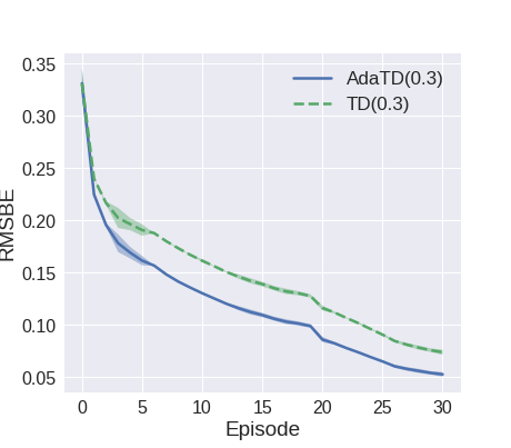
In the test of Mountain Car, the performance of all three methods is close, while AdaTD(λ\lambda) still has a small advantage over other two when λ\lambda is small. In the Acrobot task, the initial step size is relatively large for AdaTD(λ\lambda), but AdaTD(λ\lambda) is able to adjust the large initial step size and guarantee afterwards convergence. Note there is a major fluctuation in average loss around episode 3030. TD(λ\lambda) has constant step size, and thus it is more vulnerable to the fluctuation than AdaTD(λ\lambda). As a result, our algorithm demonstrates better overall convergence speed over TD(λ\lambda).

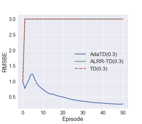
In Figures 4 and 5, we tested our algorithm with neural network parameterization. In these tests, the step size of TD(λ\lambda) cannot be large due to stability issues. As a result, TD(λ\lambda) is outperformed by AdaTD(λ\lambda) where large step size is allowed. In fact, when λ\lambda is large, a small step size of η=0.02\eta=0.02 still cannot guarantee the stability of TD(λ\lambda). It can be observed in Figure 4 that when λ\lambda gets larger, i.e. the gradient magnitude is larger, original TD(λ\lambda) becomes less stable. In comparison, AdaTD(λ\lambda) has exhibited robustness to the choice of λ\lambda and the large initial step size in this test.

We conduct two experiments in Figures 3 and 6 where we deliberately skip the step size tuning process and applies large step size to all methods. We show that our algorithm is more robust to large step size and therefore is easier to tune in practice. The hyper-parameters of the two tests are the same as before except for step sizes. In Acrobot, step size is set to 1. In Cartpole, step size is set to 0.8.

In Figure 7, we have also provided another test to evaluate the performance of AdaTD under sparse state features. The MDP has a discrete state space of size 50, and a discrete action space of size 4. The transition matrix and reward table are randomly generated with each element in (0,1)(0,1). To ensure the sparsity of gradients, we construct sparse state features as described in Section 3.3. In this test, we select η=0.45\eta=0.45 for TD, and η0=0.5\eta_{0}=0.5,δ\delta = 1.01.0, β\beta = 0.50.5 for AdaTD.

6 Proofs

6.1 Proofs for AdaTD(0)

This part contains the proofs of the main results and leaves the proofs of the technical lemmas in the appendix.

6.1.1 Technical Lemmas

Lemma 5 ([30, 22])

For 0aia¯0\leq a_{i}\leq\bar{a} and δ>0\delta>0, we have

t=1K0atδ+i=1tailn(δ+K0a¯)lnδ.\displaystyle\sum_{t=1}^{K_{0}}\frac{a_{t}}{\delta+\sum_{i=1}^{t}a_{i}}\leq\ln(\delta+K_{0}\bar{a})-\ln\delta.
Lemma 6 ([4])

For any 𝛉d{\bm{\theta}}\in\mathbb{R}^{d}, it follows

𝜽𝜽,𝐠(𝜽)(1γ)ω𝜽𝜽2.\displaystyle\langle{\bm{\theta}}^{*}-{\bm{\theta}},{\bf g}({\bm{\theta}})\rangle\geq(1-\gamma)\omega\|{\bm{\theta}}^{*}-{\bm{\theta}}\|^{2}. (25)

In the proofs, we use three shorthand notation for simplifications. Those three notation are all related to the iteration kk. Assume (𝐦k)k0({\bf m}^{k})_{k\geq 0}, (𝜽k)k0({\bm{\theta}}^{k})_{k\geq 0}, (vk)k0(v^{k})_{k\geq 0} are all generated by AdaTD(0). We denote

{𝐦^k:=𝔼[𝐦k2/(vk+δ)],Δk:=𝔼(𝜽k𝜽,𝐦k/(vk+δ)12),ϕk:=𝔼(𝜽𝜽k,𝐠(𝜽k)/(vk1+δ)12)k:=8K0(1β)δ1/2(1γ)ωh=K01𝐦^kh+ηβ𝐦^k+2RG(1β)1δ𝐠k2vk+δ+2R(1β)κρK0δ.\displaystyle\begin{cases}\hat{\bf m}_{k}&:=\mathbb{E}\Big{[}\|{\bf m}^{k}\|^{2}/(v^{k}+\delta)\Big{]},\\ \Delta_{k}&:=\mathbb{E}\left(\langle{\bm{\theta}}^{k}-{\bm{\theta}}^{*},{\bf m}^{k}\rangle/(v^{k}+\delta)^{\frac{1}{2}}\right),\\ \phi_{k}&:=\mathbb{E}\left(\langle{\bm{\theta}}^{*}-{\bm{\theta}}^{k},{\bf g}({\bm{\theta}}^{k})\rangle/(v^{k-1}+\delta)^{\frac{1}{2}}\right)\\ \Re_{k}&:=\frac{8K_{0}(1-\beta)}{\delta^{1/2}(1-\gamma)\omega}\sum_{h=K_{0}}^{1}\hat{\bf m}_{k-h}+\eta\beta\hat{\bf m}_{k}\\ &\quad+2RG(1-\beta)\frac{1}{\delta}\cdot\frac{\|{\bf g}^{k}\|^{2}}{v^{k}+\delta}+\frac{2R(1-\beta)\kappa\rho^{K_{0}}}{\sqrt{\delta}}.\end{cases} (26)

The above notations will be used in the remaining lemmas.

Lemma 7

Let (Δk)k0(\Delta_{k})_{k\geq 0} and (k)k0(\Re_{k})_{k\geq 0} be defined in (26), the following result holds for AdaTD(0)

Δk+(1β)2ϕkβΔk1+k.\displaystyle\Delta_{k}+\frac{(1-\beta)}{2}\phi_{k}\leq\beta\Delta_{k-1}+\Re_{k}. (27)

On the other hand, we can bound Δk\Delta_{k} as |Δk|η2RGδ12.|\Delta_{k}|\leq\eta\frac{2RG}{\delta^{\frac{1}{2}}}.

6.1.2 Proof of Theorem 1

Given K,K0+K,K_{0}\in\mathbb{Z}^{+} and KK01K\geq K_{0}-1, Lemma 7 tells

Δk+1β2ϕkβΔk1+k,\displaystyle\Delta_{k}+\frac{1-\beta}{2}\phi_{k}\leq\beta\Delta_{k-1}+\Re_{k},

where K0+1kKK_{0}+1\leq k\leq K. Summing together, we then get

(1β)2k=K0+1Kϕk\displaystyle\frac{(1-\beta)}{2}\sum_{k=K_{0}+1}^{K}\phi_{k}
ΔK+(β1)k=K0K1Δk+k=K0+1Kk\displaystyle\leq-\Delta_{K}+(\beta-1)\sum_{k=K_{0}}^{K-1}\Delta_{k}+\sum_{k=K_{0}+1}^{K}\Re_{k}
(β1)k=K0K1Δk+k=K0+1Kk+η2RGδ12.\displaystyle\leq(\beta-1)\sum_{k=K_{0}}^{K-1}\Delta_{k}+\sum_{k=K_{0}+1}^{K}\Re_{k}+\eta\frac{2RG}{\delta^{\frac{1}{2}}}. (28)

With direct calculations, we get

𝜽𝜽k+12\displaystyle\|{\bm{\theta}}^{*}-{\bm{\theta}}^{k+1}\|^{2}
𝜽𝜽kη𝐦k/vk+δ2\displaystyle\leq\|{\bm{\theta}}^{*}-{\bm{\theta}}^{k}-\eta{\bf m}^{k}/\sqrt{v^{k}+\delta}\|^{2}
𝜽𝜽k2+2η𝐦k,𝜽k𝜽(vk+δ)12+η2𝐦k2vk+δ.\displaystyle\leq\|{\bm{\theta}}^{*}-{\bm{\theta}}^{k}\|^{2}+\frac{2\eta\langle{\bf m}^{k},{\bm{\theta}}^{k}-{\bm{\theta}}^{*}\rangle}{(v^{k}+\delta)^{\frac{1}{2}}}+\frac{\eta^{2}\|{\bf m}^{k}\|^{2}}{v^{k}+\delta}.

Taking total condition expectation gives us

𝔼𝜽𝜽k+12𝔼𝜽𝜽k2+2ηΔk+η2𝐦^k.\displaystyle\mathbb{E}\|{\bm{\theta}}^{*}-{\bm{\theta}}^{k+1}\|^{2}\leq\mathbb{E}\|{\bm{\theta}}^{*}-{\bm{\theta}}^{k}\|^{2}+2\eta\Delta_{k}+\eta^{2}\hat{\bf m}_{k}.

That is also

k=K0K1Δk𝔼𝜽𝜽K022η+η2k=K0K1𝐦^k.\displaystyle\sum_{k=K_{0}}^{K-1}-\Delta_{k}\leq\frac{\mathbb{E}\|{\bm{\theta}}^{*}-{\bm{\theta}}^{K_{0}}\|^{2}}{2\eta}+\frac{\eta}{2}\sum_{k=K_{0}}^{K-1}\hat{\bf m}_{k}.

Combining (6.1.2), we are then led to

k=K0+1Kϕk\displaystyle\sum_{k=K_{0}+1}^{K}\phi_{k}
2k=K0K1(Δk)+21βk=K0+1Kk+4RGηδ12(1β)\displaystyle\leq 2\sum_{k=K_{0}}^{K-1}(-\Delta_{k})+\frac{2}{1-\beta}\sum_{k=K_{0}+1}^{K}\Re_{k}+\frac{4RG\eta}{\delta^{\frac{1}{2}}(1-\beta)}
𝔼𝜽𝜽K02η+ηk=K0K1𝐦^k\displaystyle\leq\frac{\mathbb{E}\|{\bm{\theta}}^{*}-{\bm{\theta}}^{K_{0}}\|^{2}}{\eta}+\eta\sum_{k=K_{0}}^{K-1}\hat{\bf m}_{k}
+k=K0+1K2k1β+4RGηδ12(1β)\displaystyle\qquad+\sum_{k=K_{0}+1}^{K}\frac{2\Re_{k}}{1-\beta}+\frac{4RG\eta}{\delta^{\frac{1}{2}}(1-\beta)}
4R2η+ηk=K0K1𝐦^k+k=K0+1K2k1β+4RGηδ12(1β).\displaystyle\leq\frac{4R^{2}}{\eta}+\eta\sum_{k=K_{0}}^{K-1}\hat{\bf m}_{k}+\sum_{k=K_{0}+1}^{K}\frac{2\Re_{k}}{1-\beta}+\frac{4RG\eta}{\delta^{\frac{1}{2}}(1-\beta)}. (29)

Now, we turn to bound the right side of (6.1.2): with the definition of k\Re_{k},

ηk=K0K1𝐦^k+21βk=K0+1Kk\displaystyle\eta\sum_{k=K_{0}}^{K-1}\hat{\bf m}_{k}+\frac{2}{1-\beta}\sum_{k=K_{0}+1}^{K}\Re_{k}
ηk=K0K1𝐦^k+(16K02δ1/2(1γ)ω+2ηβ1β)k=K0+1K𝐦^k\displaystyle\leq\eta\sum_{k=K_{0}}^{K-1}\hat{\bf m}_{k}+\left(\frac{16K_{0}^{2}}{\delta^{1/2}(1-\gamma)\omega}+\frac{2\eta\beta}{1-\beta}\right)\sum_{k=K_{0}+1}^{K}\hat{\bf m}_{k}
+4RGδk=K0+1K𝐠k2vk+δ+4RκρK0δ(KK0).\displaystyle\qquad+\frac{4RG}{\delta}\sum_{k=K_{0}+1}^{K}\frac{\|{\bf g}^{k}\|^{2}}{v^{k}+\delta}+\frac{4R\kappa\rho^{K_{0}}}{\sqrt{\delta}}(K-K_{0}).

With Lemma 4, the bound is further bounded by

(η+16K02δ1/2(1γ)ω+2ηβ1β)k=1K𝐦^k\displaystyle\left(\eta+\frac{16K_{0}^{2}}{\delta^{1/2}(1-\gamma)\omega}+\frac{2\eta\beta}{1-\beta}\right)\sum_{k=1}^{K}\hat{\bf m}_{k}
+4RGδk=1K𝐠k2vk+δ+4RκρK0δ(KK0)\displaystyle\qquad+\frac{4RG}{\delta}\sum_{k=1}^{K}\frac{\|{\bf g}^{k}\|^{2}}{v^{k}+\delta}+\frac{4R\kappa\rho^{K_{0}}}{\sqrt{\delta}}(K-K_{0})
Lemma4(16K02δ1/2(1γ)ω+2ηβ1β+η)\displaystyle\overset{\textrm{Lemma}~{}\ref{core0}}{\leq}\left(\frac{16K_{0}^{2}}{\delta^{1/2}(1-\gamma)\omega}+\frac{2\eta\beta}{1-\beta}+\eta\right)
×ln(δ+(K1)G2δ)\displaystyle\qquad\times\ln(\frac{\delta+(K-1)G^{2}}{\delta})
+4RGδln(δ+KG2δ)+4RκρK0δ(KK0),\displaystyle\qquad+\frac{4RG}{\delta}\ln(\frac{\delta+KG^{2}}{\delta})+\frac{4R\kappa\rho^{K_{0}}}{\sqrt{\delta}}(K-K_{0}), (30)

where we used the inequality k=1K𝐠k2vk+δln(δ+KG2δ)\sum_{k=1}^{K}\frac{\|{\bf g}^{k}\|^{2}}{v^{k}+\delta}\leq\ln(\frac{\delta+KG^{2}}{\delta}) (Lemma 5). We set K0=lnK/ln1ρK_{0}=\ulcorner\ln K/\ln\frac{1}{\rho}\urcorner. It is easy to see that K94(K0+1)K\geq\frac{9}{4}(K_{0}+1) as KK is large. On the other hand, with Lemma 6, we can get

k=K0Kϕk\displaystyle\sum_{k=K_{0}}^{K}\phi_{k} k=K0K(1γ)ω𝔼𝜽𝜽k2[(k1)G2+δ]12\displaystyle\geq\sum_{k=K_{0}}^{K}\frac{(1-\gamma)\omega\mathbb{E}\|{\bm{\theta}}^{*}-{\bm{\theta}}^{k}\|^{2}}{[(k-1)G^{2}+\delta]^{\frac{1}{2}}}
2((K1)G2+δ(K01)G2+δ)/G2\displaystyle\geq 2\Big{(}\sqrt{(K-1)G^{2}+\delta}-\sqrt{(K_{0}-1)G^{2}+\delta}\Big{)}/G^{2}
×(1γ)ωminK0kK𝔼𝜽𝜽k2\displaystyle\qquad\!\times(1-\gamma)\omega\min_{K_{0}\leq k\leq K}\mathbb{E}\|{\bm{\theta}}^{*}-{\bm{\theta}}^{k}\|^{2}
(1γ)ωK/GminK0kK𝔼𝜽𝜽k2,\displaystyle\geq(1-\gamma)\omega\sqrt{K}/G\cdot\min_{K_{0}\leq k\leq K}\mathbb{E}\|{\bm{\theta}}^{*}-{\bm{\theta}}^{k}\|^{2}, (31)

where we used K94(K0+1)K\geq\frac{9}{4}(K_{0}+1) to get

2((K1)G2+δ(K01)G2+δ)KG.2(\sqrt{(K-1)G^{2}+\delta}-\sqrt{(K_{0}-1)G^{2}+\delta})\geq\sqrt{K}G.

In this case, we then derive

(1γ)ωmin1kK𝔼𝜽𝜽k2\displaystyle(1-\gamma)\omega\min_{1\leq k\leq K}\mathbb{E}\|{\bm{\theta}}^{*}-{\bm{\theta}}^{k}\|^{2}
(1γ)ωminK0kK𝔼𝜽𝜽k2\displaystyle\leq(1-\gamma)\omega\min_{K_{0}\leq k\leq K}~{}\mathbb{E}\|{\bm{\theta}}^{*}-{\bm{\theta}}^{k}\|^{2}
4RκρK0GδK+(16K02Gδ1/2(1γ)ω+2Gηβ(1β)+ηG\displaystyle\leq\frac{4R\kappa\rho^{K_{0}}G}{\sqrt{\delta}}\sqrt{K}+\Big{(}\frac{16K_{0}^{2}G}{\delta^{1/2}(1-\gamma)\omega}+\frac{2G\eta\beta}{(1-\beta)}+\eta G
+4RG2δ)×ln(δ+KG2δ)1K+(4R2Gη+4RG2ηδ12(1β))1K.\displaystyle+\frac{4RG^{2}}{\delta}\Big{)}\times\ln(\frac{\delta+KG^{2}}{\delta})\frac{1}{\sqrt{K}}+(\frac{4R^{2}G}{\eta}+\frac{4RG^{2}\eta}{\delta^{\frac{1}{2}}(1-\beta)})\frac{1}{\sqrt{K}}.

By setting K0:=lnK/ln1ρK_{0}:=\ulcorner\ln K/\ln\frac{1}{\rho}\urcorner and defining the constants involved in the theorem as given in Theorem 1. we then proved the results.

6.1.3 Proof of Theorem 2

The proof lies on a re-estimate of (6.1.2). Under condition (20), we can derive

k=K0Kϕk\displaystyle\sum_{k=K_{0}}^{K}\phi_{k} k=K0K(1γ)ω𝔼𝜽𝜽k2[vk1+δ]12\displaystyle\geq\sum_{k=K_{0}}^{K}\frac{(1-\gamma)\omega\mathbb{E}\|{\bm{\theta}}^{*}-{\bm{\theta}}^{k}\|^{2}}{[v^{k-1}+\delta]^{\frac{1}{2}}}
k=K0K(1γ)ω[c(k1)ν+δ]12×minK0kK𝔼𝜽𝜽k2\displaystyle\geq\sum_{k=K_{0}}^{K}\frac{(1-\gamma)\omega}{[c(k-1)^{\nu}+\delta]^{\frac{1}{2}}}\!\times\min_{K_{0}\leq k\leq K}\mathbb{E}\|{\bm{\theta}}^{*}-{\bm{\theta}}^{k}\|^{2}
K1ν2(1γ)ω2(1ν/2)cminK0kK𝔼𝜽𝜽k2,\displaystyle\geq\frac{K^{1-\frac{\nu}{2}}(1-\gamma)\omega}{2(1-\nu/2)\sqrt{c}}\cdot\min_{K_{0}\leq k\leq K}\mathbb{E}\|{\bm{\theta}}^{*}-{\bm{\theta}}^{k}\|^{2}, (32)

as K211ν/2K0K\geq 2^{\frac{1}{1-\nu/2}}K_{0}. Noticing that (6.1.2) still holds, which means

min1kK𝔼𝜽𝜽k2=O(K02lnKK1ν2+ρK0Kν2).\min_{1\leq k\leq K}\mathbb{E}\|{\bm{\theta}}^{*}-{\bm{\theta}}^{k}\|^{2}=O(\frac{K_{0}^{2}\ln K}{K^{1-\frac{\nu}{2}}}+\rho^{K_{0}}K^{\frac{\nu}{2}}).

To achieve the O(ϵ)O(\epsilon)-accuracy for min1kK{𝔼𝜽𝜽k2}\min_{1\leq k\leq K}\{\mathbb{E}\|{\bm{\theta}}^{*}-{\bm{\theta}}^{k}\|^{2}\}, we need

ρK0Kν2ϵ,K02lnKK1ν2ϵ.\displaystyle\rho^{K_{0}}K^{\frac{\nu}{2}}\leq\epsilon,\frac{K_{0}^{2}\ln K}{K^{1-\frac{\nu}{2}}}\leq\epsilon.

We then have K0=O~(ln1ϵ/ln1ρ)K_{0}=\tilde{O}\left(\ln\frac{1}{\epsilon}/\ln\frac{1}{\rho}\right) and K=O~((ln1ϵ)21ν2/[ϵ11ν2(ln1ρ)21ν2])K=\tilde{O}\left((\ln\frac{1}{\epsilon})^{\frac{2}{1-\frac{\nu}{2}}}\Big{/}[\epsilon^{\frac{1}{1-\frac{\nu}{2}}}(\ln\frac{1}{\rho})^{\frac{2}{1-\frac{\nu}{2}}}]\right).

6.2 Proofs for AdaTD(λ\lambda)

The proof of AdaTD(λ\lambda) is similar to AdaTD(0) but with involved technical lemmas being modified. The complete proof is given in the appendix.

7 Conclusions

We developed an improved variant of the celebrated TD learning algorithm in this paper. Motivated by the close link between TD(0) and stochastic gradient-based methods, we developed adaptive TD(0) and TD(λ\lambda) algorithms. The finite-time convergence analysis of the novel adaptive TD(0) and TD(λ\lambda) algorithms has been established under the Markovian observation model. While the worst-case convergence rates of Adaptive TD(0) and TD(λ\lambda) are similar to those of the original TD(0) and TD(λ\lambda), our numerical tests on several standard benchmark tasks demonstrate the effectiveness of our adaptive approaches. Future work includes variance-reduced and decentralized AdaTD approaches.

References

  • [1] R. S. Sutton, A. G. Barto, et al., Introduction to reinforcement learning, vol. 2. MIT press Cambridge, 1998.
  • [2] R. S. Sutton, “Learning to predict by the methods of temporal differences,” Machine learning, vol. 3, no. 1, pp. 9–44, 1988.
  • [3] L. Baird, “Residual algorithms: Reinforcement learning with function approximation,” in Machine Learning, pp. 30–37, 1995.
  • [4] J. N. Tsitsiklis and B. Van Roy, “An analysis of temporal-difference learning with function approximation,” IEEE transactions on automatic control, vol. 42, no. 5, pp. 674–690, 1997.
  • [5] E. Even-Dar and Y. Mansour, “Learning rates for Q-learning,” Journal of machine learning Research, vol. 5, no. Dec., pp. 1–25, 2003.
  • [6] T. Jaakkola, M. I. Jordan, and S. P. Singh, “Convergence of stochastic iterative dynamic programming algorithms,” in Advances in neural information processing systems, pp. 703–710, 1994.
  • [7] V. S. Borkar and S. P. Meyn, “The ode method for convergence of stochastic approximation and reinforcement learning,” SIAM Journal on Control and Optimization, vol. 38, no. 2, pp. 447–469, 2000.
  • [8] R. S. Sutton, H. R. Maei, and C. Szepesvári, “A convergent o(n)o(n) temporal-difference algorithm for off-policy learning with linear function approximation,” in Advances in Neural Information Processing Systems, (Vancouver, Canada), pp. 1609–1616, Dec. 2009.
  • [9] B. Liu, J. Liu, M. Ghavamzadeh, S. Mahadevan, and M. Petrik, “Finite-sample analysis of proximal gradient td algorithms.,” in Proc. Conf. Uncertainty in Artificial Intelligence, (Amsterdam, Netherlands), pp. 504–513, 2015.
  • [10] G. Dalal, B. Szörényi, G. Thoppe, and S. Mannor, “Finite sample analyses for TD(0) with function approximation,” in Thirty-Second AAAI Conference on Artificial Intelligence, pp. 6144–6153, 2018.
  • [11] C. Lakshminarayanan and C. Szepesvari, “Linear stochastic approximation: How far does constant step-size and iterate averaging go?,” in International Conference on Artificial Intelligence and Statistics, pp. 1347–1355, 2018.
  • [12] J. Bhandari, D. Russo, and R. Singal, “A finite time analysis of temporal difference learning with linear function approximation,” in arXiv:1806.02450, two-page extended abstract at COLT 2018, PMLR, 2018.
  • [13] R. Srikant and L. Ying, “Finite-time error bounds for linear stochastic approximation and TD learning,” COLT, 2019.
  • [14] B. Hu and U. Syed, “Characterizing the exact behaviors of temporal difference learning algorithms using markov jump linear system theory,” in Advances in Neural Information Processing Systems, (Vancouver, Canada), pp. 8477–8488, Dec. 2019.
  • [15] T. Doan, S. Maguluri, and J. Romberg, “Finite-time analysis of distributed TD(0) with linear function approximation on multi-agent reinforcement learning,” in International Conference on Machine Learning, pp. 1626–1635, 2019.
  • [16] A. Devraj and S. Meyn, “Zap Q-learning,” in Advances in Neural Information Processing Systems, (Long Beach, CA), pp. 2235–2244, Dec. 2017.
  • [17] L. Y. Harsh Gupta, R. Srikant, “Finite-time performance bounds and adaptive learning rate selection for two time-scale reinforcement learning,” in Advances in Neural Information Processing Systems, (Vancouver, Canada), pp. 4706–4715, Nov. 2019.
  • [18] N. Vieillard, B. Scherrer, O. Pietquin, and M. Geist, “Momentum in reinforcement learning,” in International Conference on Artificial Intelligence and Statistics, pp. 2529–2538, PMLR, 2020.
  • [19] L. Shani, Y. Efroni, and S. Mannor, “Adaptive trust region policy optimization: Global convergence and faster rates for regularized MDPs,” in Proceedings of the AAAI Conference on Artificial Intelligence, vol. 34, pp. 5668–5675, 2020.
  • [20] J. Duchi, E. Hazan, and Y. Singer, “Adaptive subgradient methods for online learning and stochastic optimization,” Journal of Machine Learning Research, vol. 12, no. Jul, pp. 2121–2159, 2011.
  • [21] H. B. McMahan and M. Streeter, “Adaptive bound optimization for online convex optimization,” COLT 2010, p. 244, 2010.
  • [22] X. Li and F. Orabona, “On the convergence of stochastic gradient descent with adaptive stepsizes,” in The 22nd International Conference on Artificial Intelligence and Statistics, pp. 983–992, PMLR, 2019.
  • [23] R. Ward, X. Wu, and L. Bottou, “Adagrad stepsizes: Sharp convergence over nonconvex landscapes,” in International Conference on Machine Learning, pp. 6677–6686, PMLR, 2019.
  • [24] T. Tieleman and G. Hinton, “Rmsprop: Neural networks for machine learning,” University of Toronto, Technical Report, 2012.
  • [25] M. D. Zeiler, “ADADELTA: An adaptive learning rate method,” arXiv preprint:1212.5701, Dec. 2012.
  • [26] D. P. Kingma and J. Ba, “Adam: A method for stochastic optimization,” ICLR, 2014.
  • [27] T. Dozat, “Incorporating nesterov momentum into adam,” 2016.
  • [28] S. J. Reddi, S. Kale, and S. Kumar, “On the convergence of adam and beyond,” ICLR, 2019.
  • [29] F. Zou, L. Shen, Z. Jie, W. Zhang, and W. Liu, “A sufficient condition for convergences of adam and rmsprop,” in Proceedings of the IEEE Conference on Computer Vision and Pattern Recognition, pp. 11127–11135, 2019.
  • [30] X. Chen, S. Liu, R. Sun, and M. Hong, “On the convergence of a class of adam-type algorithms for non-convex optimization,” ICLR, 2018.
  • [31] D. A. Levin and Y. Peres, Markov chains and mixing times, vol. 107. American Mathematical Soc., 2017.
  • [32] V. Mnih, K. Kavukcuoglu, D. Silver, A. A. Rusu, J. Veness, M. G. Bellemare, A. Graves, M. Riedmiller, A. K. Fidjeland, G. Ostrovski, et al., “Human-level control through deep reinforcement learning,” Nature, vol. 518, no. 7540, p. 529, 2015.
  • [33] L. Liao, L. Shen, J. Duan, M. Kolar, and D. Tao, “Local adagrad-type algorithm for stochastic convex-concave minimax problems,” arXiv preprint arXiv:2106.10022, 2021.
  • [34] Z. Chen, Z. Yuan, J. Yi, B. Zhou, E. Chen, and T. Yang, “Universal stagewise learning for non-convex problems with convergence on averaged solutions,” in International Conference on Learning Representations, 2018.
  • [35] M. Liu, Y. Mroueh, J. Ross, W. Zhang, X. Cui, P. Das, and T. Yang, “Towards better understanding of adaptive gradient algorithms in generative adversarial nets,” in International Conference on Learning Representations, 2019.
  • [36] R. Mendelssohn, “An iterative aggregation procedure for markov decision processes,” Operations Research, vol. 30, no. 1, pp. 62–73, 1982.
  • [37] D. P. Bertsekas and D. A. Castanon, “Adaptive aggregation methods for infinite horizon dynamic programming,” IEEE Transactions on Automatic Control, vol. 34, no. 6, pp. 589–598, 1989.
  • [38] D. Abel, D. Hershkowitz, and M. Littman, “Near optimal behavior via approximate state abstraction,” in International Conference on Machine Learning, pp. 2915–2923, PMLR, 2016.
  • [39] Y. Duan, T. Ke, and M. Wang, “State aggregation learning from markov transition data,” Advances in Neural Information Processing Systems, vol. 32, pp. 4486–4495, 2019.
  • [40] L. Li, T. J. Walsh, and M. L. Littman, “Towards a unified theory of state abstraction for mdps.,” ISAIM, vol. 4, p. 5, 2006.
  • [41] B. Van Roy, “Performance loss bounds for approximate value iteration with state aggregation,” Mathematics of Operations Research, vol. 31, no. 2, pp. 234–244, 2006.
  • [42] R. S. Sutton, “Generalization in reinforcement learning: Successful examples using sparse coarse coding,” Advances in neural information processing systems, pp. 1038–1044, 1996.
  • [43] B. Van Roy, Learning and value function approximation in complex decision processes. PhD thesis, Massachusetts Institute of Technology, 1998.
  • [44] D. P. Bertsekas, “Dynamic programming and optimal control 3rd edition, volume ii,” Belmont, MA: Athena Scientific, 2011.
  • [45] G. Brockman, V. Cheung, L. Pettersson, J. Schneider, J. Schulman, J. Tang, and W. Zaremba, “OpenAI Gym,” arXiv:1606.01540, 2016.
  • [46] R. Lowe, Y. I. Wu, A. Tamar, J. Harb, O. P. Abbeel, and I. Mordatch, “Multi-agent actor-critic for mixed cooperative-competitive environments,” in Advances in neural information processing systems, pp. 6379–6390, 2017.

8 Proofs of Technical Lemmas for AdaTD(0)

8.1 Proof of Lemma 2

Given a fixed integer K0K_{0}, with Assumptions 1 and 2, by using a shorthand notation

Ξ:=((s,s)+γϕ(s)𝜽kK0ϕ(s)𝜽kK0)ϕ(s),\Xi:=\left(\mathcal{R}(s,s^{\prime})+\gamma\phi(s^{\prime})^{\top}{\bm{\theta}}^{k-K_{0}}-\phi(s)^{\top}{\bm{\theta}}^{k-K_{0}}\right)\phi(s),

we have

𝔼(𝐠¯(𝜽kK0;sk,sk+1)σkK0)=s,s𝒮π(s)𝒫(s|s)Ξ\displaystyle\mathbb{E}(\overline{{\bf g}}({\bm{\theta}}^{k-K_{0}};s_{k},s_{k+1})\mid\sigma^{k-K_{0}})=\sum_{s,s^{\prime}\in\mathcal{S}}\pi(s)\cdot\mathcal{P}(s^{\prime}|s)\cdot\Xi
+s,s𝒮(𝒫(skskK0=s)π(s))𝒫(s|s)Ξ.\displaystyle+\sum_{s,s^{\prime}\in\mathcal{S}}(\mathcal{P}(s_{k}\mid s_{k-K_{0}}=s)-\pi(s))\cdot\mathcal{P}(s^{\prime}|s)\cdot\Xi. (33)

Noticing that the following expectation

s,s𝒮π(s)𝒫(s|s)Ξ=𝐠(𝜽kK0).\displaystyle\sum_{s,s^{\prime}\in\mathcal{S}}\pi(s)\cdot\mathcal{P}(s^{\prime}|s)\cdot\Xi={\bf g}({\bm{\theta}}^{k-K_{0}}).

With Assumption 2, the second term in right side of (8.1) then can be bounded by Sκ¯(B+Rγ+R)ρK0S\bar{\kappa}(B+R\gamma+R)\rho^{K_{0}}. By setting κ:=Sκ¯(B+Rγ+R)\kappa:=S\bar{\kappa}(B+R\gamma+R) and using 𝔼(𝔼(σ))=𝔼()\mathbb{E}(\mathbb{E}(\cdot\mid\sigma))=\mathbb{E}(\cdot), we then proved the result.

8.2 Proof of Lemma 3

With the fact

𝐠k=𝐠(𝜽k)+𝐠k𝐠¯(𝜽kK0;sk,sk+1)\displaystyle{\bf g}^{k}={\bf g}({\bm{\theta}}^{k})+{\bf g}^{k}-\overline{{\bf g}}({\bm{\theta}}^{k-K_{0}};s_{k},s_{k+1})
+𝐠¯(𝜽kK0;sk,sk+1)𝐠(𝜽kK0)+𝐠(𝜽kK0)𝐠(𝜽k),\displaystyle+\overline{{\bf g}}({\bm{\theta}}^{k-K_{0}};s_{k},s_{k+1})-{\bf g}({\bm{\theta}}^{k-K_{0}})+{\bf g}({\bm{\theta}}^{k-K_{0}})-{\bf g}({\bm{\theta}}^{k}),

it then follows

𝔼[𝜽k𝜽,𝐠k/(vk1+δ)12]\displaystyle\mathbb{E}\Big{[}\langle{\bm{\theta}}^{k}-{\bm{\theta}}^{*},{\bf g}^{k}\rangle/(v^{k-1}+\delta)^{\frac{1}{2}}\Big{]}
=𝔼[𝜽k𝜽,𝐠(𝜽k)/(vk1+δ)12]+I+II+III,\displaystyle=\mathbb{E}\Big{[}\langle{\bm{\theta}}^{k}-{\bm{\theta}}^{*},{\bf g}({\bm{\theta}}^{k})\rangle/(v^{k-1}+\delta)^{\frac{1}{2}}\Big{]}+\textrm{I}+\textrm{II}+\textrm{III}, (34)

where

{I:=𝔼𝜽k𝜽,[𝐠k𝐠¯(𝜽kK0;sk,sk+1)](vk1+δ)12,II:=𝔼𝜽k𝜽,[𝐠¯(𝜽kK0;sk,sk+1)𝐠(𝜽kK0)](vk1+δ)12,III:=𝔼𝜽k𝜽,[𝐠(𝜽kK0)𝐠(𝜽k)](vk1+δ)12.\displaystyle\begin{cases}\textrm{I}&:=\frac{\mathbb{E}\mid\langle{\bm{\theta}}^{k}-{\bm{\theta}}^{*},\left[{\bf g}^{k}-\overline{{\bf g}}({\bm{\theta}}^{k-K_{0}};s_{k},s_{k+1})\right]\rangle\mid}{(v^{k-1}+\delta)^{\frac{1}{2}}},\\ \textrm{II}&:=\frac{\mathbb{E}\mid\langle{\bm{\theta}}^{k}-{\bm{\theta}}^{*},\left[\overline{{\bf g}}({\bm{\theta}}^{k-K_{0}};s_{k},s_{k+1})-{\bf g}({\bm{\theta}}^{k-K_{0}})\right]\rangle\mid}{(v^{k-1}+\delta)^{\frac{1}{2}}},\\ \textrm{III}&:=\frac{\mathbb{E}\mid\langle{\bm{\theta}}^{k}-{\bm{\theta}}^{*},\left[{\bf g}({\bm{\theta}}^{k-K_{0}})-{\bf g}({\bm{\theta}}^{k})\right]\rangle\mid}{(v^{k-1}+\delta)^{\frac{1}{2}}}.\end{cases}

Now, we bound I, II and III. Note that I and III enjoy the same upper bound as

I(III)2𝔼[𝜽k𝜽𝜽k𝜽kK0/(vk1+δ)12].\displaystyle\textrm{I}(\textrm{III})\leq 2\mathbb{E}\Big{[}\|{\bm{\theta}}^{k}-{\bm{\theta}}^{*}\|\cdot\|{\bm{\theta}}^{k}-{\bm{\theta}}^{k-K_{0}}\|/(v^{k-1}+\delta)^{\frac{1}{2}}\Big{]}.

With Lemma 2, we have II2RκρK0δ.\textrm{II}\leq\frac{2R\kappa\rho^{K_{0}}}{\sqrt{\delta}}. Thus, we get

I+II+III\displaystyle\textrm{I}+\textrm{II}+\textrm{III}
4h=1K0𝔼[𝜽k𝜽𝜽k+1h𝜽kh](vk1+δ)12+2RκρK0δ\displaystyle\leq 4\sum_{h=1}^{K_{0}}\frac{\mathbb{E}\Big{[}\|{\bm{\theta}}^{k}-{\bm{\theta}}^{*}\|\cdot\|{\bm{\theta}}^{k+1-h}-{\bm{\theta}}^{k-h}\|\Big{]}}{(v^{k-1}+\delta)^{\frac{1}{2}}}+\frac{2R\kappa\rho^{K_{0}}}{\sqrt{\delta}}
4h=1K0𝔼[𝜽k𝜽𝐦kh](vk1+δ)12(vkh+δ)12+2RκρK0δ.\displaystyle\leq 4\sum_{h=1}^{K_{0}}\frac{\mathbb{E}\Big{[}\|{\bm{\theta}}^{k}-{\bm{\theta}}^{*}\|\cdot\|{\bf m}^{k-h}\|\Big{]}}{(v^{k-1}+\delta)^{\frac{1}{2}}(v^{k-h}+\delta)^{\frac{1}{2}}}+\frac{2R\kappa\rho^{K_{0}}}{\sqrt{\delta}}. (35)

On the other hand, with the Cauchy-Schwarz inequality, we have

h=1K0𝔼(𝜽k𝜽𝐦kh(vk1+δ)12(vkh+δ)12σk)\displaystyle\sum_{h=1}^{K_{0}}\mathbb{E}\left(\frac{\|{\bm{\theta}}^{k}-{\bm{\theta}}^{*}\|\cdot\|{\bf m}^{k-h}\|}{(v^{k-1}+\delta)^{\frac{1}{2}}\cdot(v^{k-h}+\delta)^{\frac{1}{2}}}\mid\sigma^{k}\right)
1δ1/4h=1K0𝜽k𝜽(vk1+δ)1/4𝐦kh(vkh+δ)1/2\displaystyle\leq\frac{1}{\delta^{1/4}}\sum_{h=1}^{K_{0}}\frac{\|{\bm{\theta}}^{k}-{\bm{\theta}}^{*}\|}{(v^{k-1}+\delta)^{1/4}}\cdot\frac{\|{\bf m}^{k-h}\|}{(v^{k-h}+\delta)^{1/2}}
12δ1/4h=1K0[δ1/4(1γ)ω4K0𝜽k𝜽2(vk1+δ)1/2\displaystyle\leq\frac{1}{2\delta^{1/4}}\sum_{h=1}^{K_{0}}\Big{[}\frac{\delta^{1/4}(1-\gamma)\omega}{4K_{0}}\frac{\|{\bm{\theta}}^{k}-{\bm{\theta}}^{*}\|^{2}}{(v^{k-1}+\delta)^{1/2}}
+4K0δ1/4(1γ)ω𝐦kh2(vkh+δ)]\displaystyle\qquad+\frac{4K_{0}}{\delta^{1/4}(1-\gamma)\omega}\frac{\|{\bf m}^{k-h}\|^{2}}{(v^{k-h}+\delta)}\Big{]}
=(1γ)ω8𝜽k𝜽2(vk1+δ)1/2+2K0h=K01𝐦kh2(vkh+δ)δ1/2(1γ)ω\displaystyle=\frac{(1-\gamma)\omega}{8}\frac{\|{\bm{\theta}}^{k}-{\bm{\theta}}^{*}\|^{2}}{(v^{k-1}+\delta)^{1/2}}+\frac{2K_{0}\sum_{h=K_{0}}^{1}\frac{\|{\bf m}^{k-h}\|^{2}}{(v^{k-h}+\delta)}}{\delta^{1/2}(1-\gamma)\omega}
18𝜽𝜽k,𝐠(𝜽k)(vk1+δ)1/2+2K0h=K01𝐦kh2(vkh+δ)δ1/2(1γ)ω.\displaystyle\leq\frac{1}{8}\frac{\langle{\bm{\theta}}^{*}-{\bm{\theta}}^{k},{\bf g}({\bm{\theta}}^{k})\rangle}{(v^{k-1}+\delta)^{1/2}}+\frac{2K_{0}\sum_{h=K_{0}}^{1}\frac{\|{\bf m}^{k-h}\|^{2}}{(v^{k-h}+\delta)}}{\delta^{1/2}(1-\gamma)\omega}. (36)

Combining (8.2), (8.2) and (8.2), we then get the result.

8.3 Proof of Lemma 4

For simplicity, we define 𝐠k:=𝐠¯(𝜽k;sk,sk+1){\bf g}^{k}:=\overline{{\bf g}}({\bm{\theta}}^{k};s_{k},s_{k+1}). Recall 𝐦k=(1β)j=1k1βk1j𝐠j.{\bf m}^{k}=(1-\beta)\sum_{j=1}^{k-1}\beta^{k-1-j}{\bf g}^{j}. We have

𝐦k2/(vk+δ)\displaystyle\|{\bf m}^{k}\|^{2}/(v^{k}+\delta)
(1β)2j=1k1βk1j𝐠j/(vk+δ)122\displaystyle\leq(1-\beta)^{2}\|\sum_{j=1}^{k-1}\beta^{k-1-j}{\bf g}^{j}/(v^{k}+\delta)^{\frac{1}{2}}\|^{2}
a)(1β)2(j=1k1βk1j)j=1k1βk1j𝐠j2/(vk+δ)\displaystyle\overset{a)}{\leq}(1-\beta)^{2}(\sum_{j=1}^{k-1}\beta^{k-1-j})\cdot\sum_{j=1}^{k-1}\beta^{k-1-j}\|{\bf g}^{j}\|^{2}/(v^{k}+\delta)
=(1β)j=1k1βk1j𝐠j2/(vk+δ)\displaystyle=(1-\beta)\cdot\sum_{j=1}^{k-1}\beta^{k-1-j}\|{\bf g}^{j}\|^{2}/(v^{k}+\delta)
=b)(1β)j=1k1βk1j𝐠j2/(vj+δ)\displaystyle\overset{b)}{=}(1-\beta)\cdot\sum_{j=1}^{k-1}\beta^{k-1-j}\|{\bf g}^{j}\|^{2}/(v^{j}+\delta)

where a)a) uses the fact (j=1k1ajbj)2j=1k1aj2j=1k1bj2(\sum_{j=1}^{k-1}a_{j}b_{j})^{2}\leq\sum_{j=1}^{k-1}a_{j}^{2}\sum_{j=1}^{k-1}b_{j}^{2} with aj=βk1j2a_{j}=\beta^{\frac{k-1-j}{2}} and bj=βk1j2𝐠j/(vk+δ)12b_{j}=\beta^{\frac{k-1-j}{2}}{\bf g}^{j}/(v^{k}+\delta)^{\frac{1}{2}}, and b)b) is due to vjvkv^{j}\leq v^{k} when jk1j\leq k-1. Then, we then get

k=1Kj=1k1βk1j𝐠j2/(vj+δ)\displaystyle\sum_{k=1}^{K}\sum_{j=1}^{k-1}\beta^{k-1-j}\|{\bf g}^{j}\|^{2}/(v^{j}+\delta)
=j=1K1k=jK1βkj𝐠j2/(vj+δ)j=1K1𝐠j2/(vj+δ).\displaystyle=\sum_{j=1}^{K-1}\sum_{k=j}^{K-1}\beta^{k-j}\|{\bf g}^{j}\|^{2}/(v^{j}+\delta)\leq\sum_{j=1}^{K-1}\|{\bf g}^{j}\|^{2}/(v^{j}+\delta).

Combining the inequalities above, we then get the result. By applying Lemma 5, we then get the second bound.

8.4 Proof of Lemma 7

With direct computations, we have

Δk\displaystyle\Delta_{k} =𝔼(𝜽k𝜽,𝐦k/(vk1+δ)12)I\displaystyle=\underbrace{\mathbb{E}\left(\langle{\bm{\theta}}^{k}-{\bm{\theta}}^{*},{\bf m}^{k}\rangle/(v^{k-1}+\delta)^{\frac{1}{2}}\right)}_{\textrm{I}}
+𝔼(𝜽k𝜽,𝐦k(vk+δ)12𝜽k𝜽,𝐦k(vk1+δ)12)II\displaystyle\quad+\underbrace{\mathbb{E}\left(\frac{\langle{\bm{\theta}}^{k}-{\bm{\theta}}^{*},{\bf m}^{k}\rangle}{(v^{k}+\delta)^{\frac{1}{2}}}-\frac{\langle{\bm{\theta}}^{k}-{\bm{\theta}}^{*},{\bf m}^{k}\rangle}{(v^{k-1}+\delta)^{\frac{1}{2}}}\right)}_{\textrm{II}}

Now, we bound I and II. The Cauchy’s inequality then gives us

II 𝜽k𝜽𝐦k(1/(vk1+δ)121/(vk+δ)12)\displaystyle\leq\|{\bm{\theta}}^{k}-{\bm{\theta}}^{*}\|\cdot\|{\bf m}^{k}\|\cdot(1/(v^{k-1}+\delta)^{\frac{1}{2}}-1/(v^{k}+\delta)^{\frac{1}{2}})
2RG𝐠k2(vk+δ)12(vk1+δ)12((vk+δ)12+(vk1+δ)12)\displaystyle\leq 2RG\frac{\|{\bf g}^{k}\|^{2}}{(v^{k}+\delta)^{\frac{1}{2}}(v^{k-1}+\delta)^{\frac{1}{2}}((v^{k}+\delta)^{\frac{1}{2}}+(v^{k-1}+\delta)^{\frac{1}{2}})}
=2RGδ𝐠k2vk+δ.\displaystyle=\frac{2RG}{\delta}\cdot\frac{\|{\bf g}^{k}\|^{2}}{v^{k}+\delta}.

With scheme of the algorithm, we use a shorthand notation Λ:=𝔼(𝜽k𝜽,𝐠k/(vk1+δ)12σk)\Lambda:=\mathbb{E}(\langle{\bm{\theta}}^{k}-{\bm{\theta}}^{*},{\bf g}^{k}\rangle/(v^{k-1}+\delta)^{\frac{1}{2}}\mid\sigma^{k}) and then get

I=𝔼(𝜽k𝜽,β𝐦k1+(1β)𝐠k/(vk1+δ)12)\displaystyle\textrm{I}=\mathbb{E}\left(\langle{\bm{\theta}}^{k}-{\bm{\theta}}^{*},\beta{\bf m}^{k-1}+(1-\beta){\bf g}^{k}\rangle/(v^{k-1}+\delta)^{\frac{1}{2}}\right)
=(β1)Λ+β𝜽k𝜽,𝐦k1/(vk1+δ)12\displaystyle=(\beta-1)\Lambda+\beta\langle{\bm{\theta}}^{k}-{\bm{\theta}}^{*},{\bf m}^{k-1}\rangle/(v^{k-1}+\delta)^{\frac{1}{2}}
=(β1)Λ+βΔk+β𝜽k𝜽k1,𝐦k1/(vk1+δ)12\displaystyle=(\beta-1)\Lambda+\beta\Delta_{k}+\beta\langle{\bm{\theta}}^{k}-{\bm{\theta}}^{k-1},{\bf m}^{k-1}\rangle/(v^{k-1}+\delta)^{\frac{1}{2}}
a)(β1)Λ+βΔk+β𝜽k1𝜽k𝐦k1/(vk1+δ)12\displaystyle\overset{a)}{\leq}(\beta-1)\Lambda+\beta\Delta_{k}+\beta\|{\bm{\theta}}^{k-1}-{\bm{\theta}}^{k}\|\cdot\|{\bf m}^{k-1}\|/(v^{k-1}+\delta)^{\frac{1}{2}}
b)(β1)Λ+βΔk+ηβ𝐦k12/(vk1+δ),\displaystyle\overset{b)}{\leq}(\beta-1)\Lambda+\beta\Delta_{k}+\eta\beta\|{\bf m}^{k-1}\|^{2}/(v^{k-1}+\delta),

where a)a) uses the Cauchy’s inequality, b)b) depends on the scheme of AdaTD(0). Combination of the inequalities I, II and Lemma 3 gives the final result.

The bound for Δk\Delta_{k} a direct result from the bound of 𝐦k{\bf m}^{k} and 𝐠k{\bf g}^{k}.

9 Proofs for AdaTD(λ\lambda)

9.1 Technical Lemmas

Although (𝐦k)k0({\bf m}^{k})_{k\geq 0} and (vk)k0(v^{k})_{k\geq 0} are generated as the same as AdaTD(0), the difference scheme of updating (𝐠k)k0({\bf g}^{k})_{k\geq 0} makes they different. Thus, we use different notation here. Like previous proofs, we denote three items for AdaTD(λ\lambda) as follows

{𝐦^^k:=𝔼[𝐦k2/(vk+δ)],Δ^k:=𝔼(𝜽k𝜽,𝐦k/(vk+δ)12),ϕ^k:=𝔼(𝜽𝜽k,𝐠λ(𝜽k)/(vk1+δ)12),^k:=8K0(1β)δ1/2(1γ)ω(1γλ)d=K01𝐦^^kd+2R(1β)κρK0δ(1γλ)+2RG^(1β)dδ𝐠k2vk+δ+2R(1β)G^δ(1γλ)ζk+ηβ𝐦^^k.\displaystyle\begin{cases}\hat{\hat{{\bf m}}}_{k}&:=\mathbb{E}\Big{[}\|{\bf m}^{k}\|^{2}/(v^{k}+\delta)\Big{]},\\ \hat{\Delta}_{k}&:=\mathbb{E}\left(\langle{\bm{\theta}}^{k}-{\bm{\theta}}^{*},{\bf m}^{k}\rangle/(v^{k}+\delta)^{\frac{1}{2}}\right),\\ \hat{\phi}_{k}&:=\mathbb{E}\left(\langle{\bm{\theta}}^{*}-{\bm{\theta}}^{k},{\bf g}^{\lambda}({\bm{\theta}}^{k})\rangle/(v^{k-1}+\delta)^{\frac{1}{2}}\right),\\ \hat{\Re}_{k}&:=\frac{8K_{0}(1-\beta)}{\delta^{1/2}(1-\gamma)\omega(1-\gamma\lambda)}\sum_{d=K_{0}}^{1}\hat{\hat{{\bf m}}}_{k-d}+\frac{2R(1-\beta)\kappa\rho^{K_{0}}}{\sqrt{\delta}(1-\gamma\lambda)}\\ &+2R\hat{G}(1-\beta)\frac{d}{\delta}\cdot\frac{\|{\bf g}^{k}\|^{2}}{v^{k}+\delta}+\frac{2R(1-\beta)\hat{G}}{\sqrt{\delta}(1-\gamma\lambda)}\zeta_{k}+\eta\beta\hat{\hat{{\bf m}}}_{k}.\end{cases} (37)

Direct computing gives

k=1ζkmax{γλ,ρ}(1max{γλ,ρ})2.\displaystyle\sum_{k=1}^{\infty}\zeta_{k}\leq\frac{\max\{\gamma\lambda,\rho\}}{(1-\max\{\gamma\lambda,\rho\})^{2}}. (38)
Lemma 8

Assume (𝔼𝐳k)k0(\mathbb{E}{\bf z}^{k})_{k\geq 0} is generated by AdaTD(λ\lambda). It then holds that

𝔼𝐳k𝔼𝐳kζk1γλand𝐳11γλ.\displaystyle\|\mathbb{E}{\bf z}^{k}-\mathbb{E}{\bf z}^{\infty}\|\leq\frac{k\zeta^{k}}{1-\gamma\lambda}~{}~{}~{}{\rm and}~{}~{}~{}\|{\bf z}^{\infty}\|\leq\frac{1}{1-\gamma\lambda}. (39)
Lemma 9

Assume (𝐦k)k0({\bf m}^{k})_{k\geq 0} and (vk)k0(v^{k})_{k\geq 0} are given by (37). We have

k=1K𝐦^^kj=1K1𝔼𝐠j2/(vj+δ).\displaystyle\sum_{k=1}^{K}\hat{\hat{{\bf m}}}_{k}\leq\sum_{j=1}^{K-1}\mathbb{E}\|{\bf g}^{j}\|^{2}/(v^{j}+\delta).

Further, with the boundedness of (𝐠k)k0(\|{\bf g}^{k}\|)_{k\geq 0}, we then get

k=1K𝐦^^kln(δ+(K1)G^2δ).\displaystyle\sum_{k=1}^{K}\hat{\hat{{\bf m}}}_{k}\leq\ln(\frac{\delta+(K-1)\hat{G}^{2}}{\delta}).
Lemma 10

Assume (𝛉k)k0({\bm{\theta}}^{k})_{k\geq 0} is generated by AdaTD(λ\lambda). Given integer K0+K_{0}\in\mathbb{Z}^{+}, we then get

𝔼[𝐠¯λ(𝜽kK0;sk,sk+1,𝐳k)]𝐠λ(𝜽kK0)\displaystyle\Big{\|}\mathbb{E}\Big{[}\overline{{\bf g}}^{\lambda}({\bm{\theta}}^{k-K_{0}};s_{k},s_{k+1},{\bf z}^{k})\big{]}-{\bf g}^{\lambda}({\bm{\theta}}^{k-K_{0}})\Big{\|}
κ1γλρK0+G^1γλζk.\displaystyle\quad\leq\frac{\kappa}{1-\gamma\lambda}\rho^{K_{0}}+\frac{\hat{G}}{1-\gamma\lambda}\zeta_{k}.
Lemma 11

Assume (𝛉k)k0({\bm{\theta}}^{k})_{k\geq 0} is generated by AdaTD(λ\lambda). Given K0+K_{0}\in\mathbb{Z}^{+}, we have

𝔼[𝜽k𝜽,𝐠k(vk1+δ)12]12ϕ^k+8K0δ1/2(1γ)ω(1γλ)\displaystyle\mathbb{E}\Big{[}\frac{\langle{\bm{\theta}}^{k}-{\bm{\theta}}^{*},{\bf g}^{k}\rangle}{(v^{k-1}+\delta)^{\frac{1}{2}}}\Big{]}\leq-\frac{1}{2}\hat{\phi}_{k}+\frac{8K_{0}}{\delta^{1/2}(1-\gamma)\omega(1-\gamma\lambda)}
+2Rδ(κ1γλρK0+G^1γλζk).\displaystyle+\frac{2R}{\sqrt{\delta}}\Big{(}\frac{\kappa}{1-\gamma\lambda}\rho^{K_{0}}+\frac{\hat{G}}{1-\gamma\lambda}\zeta_{k}\Big{)}. (40)
Lemma 12

Assume 𝐦^^k,Δ^k\hat{\hat{\bf m}}_{k},\hat{\Delta}_{k} are denoted by (37), we then have the following result

Δ^k+(1β)2ϕ^kβΔ^k1+^k.\displaystyle\hat{\Delta}_{k}+\frac{(1-\beta)}{2}\hat{\phi}_{k}\leq\beta\hat{\Delta}_{k-1}+\hat{\Re}_{k}. (41)

On the other hand, we have another bound for Δ^k\hat{\Delta}_{k} as |Δ^k|η2RG^δ12.|\hat{\Delta}_{k}|\leq\eta\frac{2R\hat{G}}{\delta^{\frac{1}{2}}}.

9.2 Proof of Theorem 3

Similar to (6.1.2), we can derive

k=K0+1K𝜽𝜽k,𝐠λ(𝜽k)(vk1+δ)12𝔼𝜽𝜽K02η\displaystyle\sum_{k=K_{0}+1}^{K}\frac{\langle{\bm{\theta}}^{*}-{\bm{\theta}}^{k},{\bf g}^{\lambda}({\bm{\theta}}^{k})\rangle}{(v^{k-1}+\delta)^{\frac{1}{2}}}\leq\frac{\mathbb{E}\|{\bm{\theta}}^{*}-{\bm{\theta}}^{K_{0}}\|^{2}}{\eta}
+ηk=K0K1𝐦^^k+21βk=K0+1K^k+4R^G^ηδ12(1β).\displaystyle\quad+\eta\sum_{k=K_{0}}^{K-1}\hat{\hat{{\bf m}}}_{k}+\frac{2}{1-\beta}\sum_{k=K_{0}+1}^{K}\hat{\Re}_{k}+\frac{4\hat{R}\hat{G}\eta}{\delta^{\frac{1}{2}}(1-\beta)}. (42)

Lemma 9 give us

ηk=K0K1𝐦^^k+21βk=K0+1K^k\displaystyle\eta\sum_{k=K_{0}}^{K-1}\hat{\hat{{\bf m}}}_{k}+\frac{2}{1-\beta}\sum_{k=K_{0}+1}^{K}\hat{\Re}_{k}
ηk=K0K1𝐦^^k+(16K02δ1/2(1γ)ω+2ηβ1β)k=K0+1K𝐦^^k\displaystyle\leq\eta\sum_{k=K_{0}}^{K-1}\hat{\hat{{\bf m}}}_{k}+\left(\frac{16K_{0}^{2}}{\delta^{1/2}(1-\gamma)\omega}+\frac{2\eta\beta}{1-\beta}\right)\sum_{k=K_{0}+1}^{K}\hat{\hat{{\bf m}}}_{k}
+4RG^δk=K0+1K𝐠k2vk+δ+4RκρK0(KK0)(1γλ)δ\displaystyle\quad+\frac{4R\hat{G}}{\delta}\sum_{k=K_{0}+1}^{K}\frac{\|{\bf g}^{k}\|^{2}}{v^{k}+\delta}+\frac{4R\kappa\rho^{K_{0}}(K-K_{0})}{(1-\gamma\lambda)\sqrt{\delta}}
+k=K0K12R^G^δ(1γλ)ζk\displaystyle\quad+\sum_{k=K_{0}}^{K-1}\frac{2\hat{R}\hat{G}}{\sqrt{\delta}(1-\gamma\lambda)}\zeta_{k}

Further with Lemma 5, the right hand is bounded by

(16K02δ1/2(1γ)ω(1γλ)+2ηβ(1β)+η)×ln(δ+(K1)G^2δ)\displaystyle\Big{(}\frac{16K_{0}^{2}}{\delta^{1/2}(1-\gamma)\omega(1-\gamma\lambda)}+\frac{2\eta\beta}{(1-\beta)}+\eta\Big{)}\times\ln(\frac{\delta+(K-1)\hat{G}^{2}}{\delta})
+4R^G^δln(δ+KG^2δ)+4R^κρK0(KK0)δ(1γλ)+2R^G^k=1+ζkδ(1γλ).\displaystyle+\frac{4\hat{R}\hat{G}}{\delta}\ln(\frac{\delta+K\hat{G}^{2}}{\delta})+\frac{4\hat{R}\kappa\rho^{K_{0}}(K-K_{0})}{\sqrt{\delta}(1-\gamma\lambda)}+\frac{2\hat{R}\hat{G}\sum_{k=1}^{+\infty}\zeta_{k}}{\sqrt{\delta}(1-\gamma\lambda)}.

The rest of the proof is almost identical to the one of Theorem 1. Letting K0=lnK/ln1ρK_{0}=\ulcorner\ln K/\ln\frac{1}{\rho}\urcorner and

C1λ:=16K02G^δ1/2(1γ)(1α)ω2+2ηβG^(1β)(1α)ω\displaystyle C_{1}^{\lambda}:=\frac{16K_{0}^{2}\hat{G}}{\delta^{1/2}(1-\gamma)(1-\alpha)\omega^{2}}+\frac{2\eta\beta\hat{G}}{(1-\beta)(1-\alpha)\omega}
+ηG^(1α)ω+4RG^2δ(1α)ω=O((lnK/ln1ρ)2δ(1γλ)),\displaystyle\quad+\frac{\eta\hat{G}}{(1-\alpha)\omega}+\frac{4R\hat{G}^{2}}{\delta(1-\alpha)\omega}=O(\frac{(\ln K/\ln\frac{1}{\rho})^{2}}{\sqrt{\delta}(1-\gamma\lambda)}),
C2λ:=4R^2G^η(1α)ω+4R^G^2ηδ12(1β)(1α)ω\displaystyle C_{2}^{\lambda}:=\frac{4\hat{R}^{2}\hat{G}}{\eta(1-\alpha)\omega}+\frac{4\hat{R}\hat{G}^{2}\eta}{\delta^{\frac{1}{2}}(1-\beta)(1-\alpha)\omega}
+2R^G^2k=1+ζkδ(1γλ)(1α)ω+4R^κ¯(B+R^γ+R^)G^(1α)δω\displaystyle\quad+\frac{2\hat{R}\hat{G}^{2}\sum_{k=1}^{+\infty}\zeta_{k}}{\sqrt{\delta}(1-\gamma\lambda)(1-\alpha)\omega}+\frac{4\hat{R}\bar{\kappa}(B+\hat{R}\gamma+\hat{R})\hat{G}}{(1-\alpha)\sqrt{\delta}\omega}
=O(1δ(1β)+max{γλ,ρ}δ(1γλ)(1max{γλ,ρ})2).\displaystyle\quad=O(\frac{1}{\sqrt{\delta}(1-\beta)}+\frac{\max\{\gamma\lambda,\rho\}}{\sqrt{\delta}(1-\gamma\lambda)(1-\max\{\gamma\lambda,\rho\})^{2}}).

we then proved the results.

9.3 Proof of Proposition 1

Based on Theorem 3, in the general case, we directly get the complexity of AdaTD(λ\lambda). Beginning from (9.2), like the proof of Theorem 2, the improved complexity can be obtained with condition (20).

10 Proofs of Technical Lemmas for Ada-TD(λ\lambda)

10.1 Proof of Lemma 8

With the scheme of updating 𝐳k{\bf z}^{k}, it follows 𝔼𝐳k=t=1k(γλ)kt𝔼ϕ(st).\mathbb{E}{\bf z}^{k}=\sum_{t=1}^{k}(\gamma\lambda)^{k-t}\mathbb{E}\phi(s_{t}). Assume π0\pi^{0} is the initial probability of s0s_{0}, then 𝔼ϕ(st)=Φ𝒫tπ0\mathbb{E}\phi(s_{t})=\Phi^{\top}\mathcal{P}^{t}\pi^{0} which yields

𝔼𝐳k=t=1k(γλ)ktΦ𝒫tπ0.\mathbb{E}{\bf z}^{k}=\sum_{t=1}^{k}(\gamma\lambda)^{k-t}\Phi^{\top}\mathcal{P}^{t}\pi^{0}.

From [oldenburger1940infinite], there exists orthogonal matrix UU such that

𝒫=UDiag(1,λ2,,λS)U.\mathcal{P}=U^{\top}\textrm{Diag}(1,\lambda_{2},\ldots,\lambda_{S})U.

with λ2λS0\lambda_{2}\geq\ldots\geq\lambda_{S}\geq 0 and λ2ρ\lambda_{2}\leq\rho. Without loss of generation, we assume γλ>ρ\gamma\lambda>\rho and then derive

𝔼𝐳k=ΦUΓUπ0,\mathbb{E}{\bf z}^{k}=\Phi^{\top}U^{\top}\Gamma U\pi^{0},

where

Γ:=Diag(t=1k(γλ)kt,t=1k(γλ)ktλ2t,,t=1k(γλ)ktλSt).\Gamma:=\textrm{Diag}(\sum_{t=1}^{k}(\gamma\lambda)^{k-t},\sum_{t=1}^{k}(\gamma\lambda)^{k-t}\lambda_{2}^{t},\ldots,\sum_{t=1}^{k}(\gamma\lambda)^{k-t}\lambda_{S}^{t}).

We also see 𝔼𝐳=ΦUDiag(11γλ,0,,0)Uπ0.\mathbb{E}{\bf z}^{\infty}=\Phi^{\top}U^{\top}\textrm{Diag}(\frac{1}{1-\gamma\lambda},0,\ldots,0)U\pi^{0}. And hence, it follows

𝔼𝐳k𝔼𝐳=ΦUΓ^Uπ0,\mathbb{E}{\bf z}^{k}-\mathbb{E}{\bf z}^{\infty}=\Phi^{\top}U^{\top}\hat{\Gamma}U\pi^{0},

where

Γ^:=Diag((γλ)k1γλ,t=1k(γλ)ktλ2t,,t=1k(γλ)ktλSt).\hat{\Gamma}:=\textrm{Diag}(\frac{-(\gamma\lambda)^{k}}{1-\gamma\lambda},\sum_{t=1}^{k}(\gamma\lambda)^{k-t}\lambda_{2}^{t},\ldots,\sum_{t=1}^{k}(\gamma\lambda)^{k-t}\lambda_{S}^{t}).

For i{2,3,,S}i\in\{2,3,\ldots,S\}, t=1k(γλ)ktλStt=1k(γλ)ktρt.\sum_{t=1}^{k}(\gamma\lambda)^{k-t}\lambda_{S}^{t}\leq\sum_{t=1}^{k}(\gamma\lambda)^{k-t}\rho^{t}. It is easy to see

ζk\displaystyle\zeta_{k} :=t=1k(γλ)ktρtt=1k(max{γλ,ρ})kt(max{γλ,ρ})t\displaystyle:=\sum_{t=1}^{k}(\gamma\lambda)^{k-t}\rho^{t}\leq\sum_{t=1}^{k}(\max\{\gamma\lambda,\rho\})^{k-t}(\max\{\gamma\lambda,\rho\})^{t}
=k(max{γλ,ρ})k.\displaystyle=k(\max\{\gamma\lambda,\rho\})^{k}.

10.2 Proof of Lemma 9

This proof is identical to the one of Lemma 4 and will not be reproduced.

10.3 Proof of Lemma 10

With the boundedness, we are led to

𝔼[𝐠¯λ(𝜽kK0;sk,sk+1,𝐳k)]\displaystyle\Big{\|}\mathbb{E}\Big{[}\overline{{\bf g}}^{\lambda}({\bm{\theta}}^{k-K_{0}};s_{k},s_{k+1},{\bf z}^{k})\Big{]}
𝔼[𝐠λ(𝜽kK0;sk,sk+1,𝐳)]G^1γλkζk.\displaystyle-\mathbb{E}\Big{[}{\bf g}^{\lambda}({\bm{\theta}}^{k-K_{0}};s_{k},s_{k+1},{\bf z}^{\infty})\Big{]}\Big{\|}\leq\frac{\hat{G}}{1-\gamma\lambda}k\zeta_{k}.

By using a shorthand notation

Υ:=(s,s)+γϕ(s)𝜽kK0ϕ(s)𝜽kK0,\Upsilon:=\mathcal{R}(s,s^{\prime})+\gamma\phi(s^{\prime})^{\top}{\bm{\theta}}^{k-K_{0}}-\phi(s)^{\top}{\bm{\theta}}^{k-K_{0}},

with direct computation, we have

𝔼[𝐠¯λ(𝜽kK0;sk,sk+1,𝐳)σ(σkK0,𝐳)]\displaystyle\mathbb{E}\Big{[}\overline{{\bf g}}^{\lambda}({\bm{\theta}}^{k-K_{0}};s_{k},s_{k+1},{\bf z}^{\infty})\mid\sigma(\sigma^{k-K_{0}},{\bf z}^{\infty})\Big{]}
=s,s𝒮π(s)𝒫(s|s)Υ𝐳\displaystyle=\sum_{s,s^{\prime}\in\mathcal{S}}\pi(s)\mathcal{P}(s^{\prime}|s)\cdot\Upsilon\cdot{\bf z}^{\infty}
+s,s𝒮(𝒫(skskK0=s)π(s))𝒫(s|s)Υ𝐳.\displaystyle+\sum_{s,s^{\prime}\in\mathcal{S}}(\mathcal{P}(s_{k}\mid s_{k-K_{0}}=s)-\pi(s))\mathcal{P}(s^{\prime}|s)\cdot\Upsilon\cdot{\bf z}^{\infty}. (43)

Noticing that

s,s𝒮π(s)𝒫(s|s)Υ𝐳\displaystyle\sum_{s,s^{\prime}\in\mathcal{S}}\pi(s)\mathcal{P}(s^{\prime}|s)\cdot\Upsilon\cdot{\bf z}^{\infty}
=𝔼[𝐠λ(𝜽kK0;sk,sk+1,𝐳)σ(σkK0,𝐳)].\displaystyle=\mathbb{E}\Big{[}{\bf g}^{\lambda}({\bm{\theta}}^{k-K_{0}};s_{k},s_{k+1},{\bf z}^{\infty})\mid\sigma(\sigma^{k-K_{0}},{\bf z}^{\infty})\Big{]}.

Direct calculation gives us

s,s𝒮(𝒫(skskK0=s)π(s))𝒫(s|s)Υ𝐳\displaystyle\Big{\|}\sum_{s,s^{\prime}\in\mathcal{S}}(\mathcal{P}(s_{k}\mid s_{k-K_{0}}=s)-\pi(s))\mathcal{P}(s^{\prime}|s)\cdot\Upsilon\cdot{\bf z}^{\infty}\Big{\|}
κρK01γλ.\displaystyle\leq\frac{\kappa\rho^{K_{0}}}{1-\gamma\lambda}.

10.4 Proof of Lemma 11

Noting

𝔼[𝐠¯λ(𝜽;s^k,s^k+1,𝐳)]=𝐠λ(𝜽),\mathbb{E}\Big{[}\overline{{\bf g}}^{\lambda}({\bm{\theta}};\hat{s}_{k},\hat{s}_{k+1},{\bf z}^{\infty})\Big{]}={\bf g}^{\lambda}({\bm{\theta}}),

where (s^1,s^2,)(\hat{s}_{1},\hat{s}_{2},\ldots) is the stationary sequence. Then for any 𝜽1,𝜽2d{\bm{\theta}}^{1},{\bm{\theta}}^{2}\in\mathbb{R}^{d},

𝐠λ(𝜽1)𝐠λ(𝜽2)\displaystyle\|{\bf g}^{\lambda}({\bm{\theta}}^{1})-{\bf g}^{\lambda}({\bm{\theta}}^{2})\|
=𝔼[𝐠¯λ(𝜽1;s^k,s^k+1,𝐳)]𝔼[𝐠¯λ(𝜽2;s^k,s^k+1,𝐳)]\displaystyle=\|\mathbb{E}\Big{[}\overline{{\bf g}}^{\lambda}({\bm{\theta}}^{1};\hat{s}_{k},\hat{s}_{k+1},{\bf z}^{\infty})\Big{]}-\mathbb{E}\Big{[}\overline{{\bf g}}^{\lambda}({\bm{\theta}}^{2};\hat{s}_{k},\hat{s}_{k+1},{\bf z}^{\infty})\Big{]}\|
2𝜽1𝜽21γλ.\displaystyle\leq\frac{2\|{\bm{\theta}}^{1}-{\bm{\theta}}^{2}\|}{1-\gamma\lambda}.

With the fact 𝐠k=𝐠λ(𝜽k)+𝐠k𝐠¯λ(𝜽kK0;sk,sk+1,𝐳k)+𝐠¯λ(𝜽kK0;sk,sk+1,𝐳k)𝐠λ(𝜽kK0)+𝐠λ(𝜽kK0)𝐠λ(𝜽k){\bf g}^{k}={\bf g}^{\lambda}({\bm{\theta}}^{k})+{\bf g}^{k}-\overline{{\bf g}}^{\lambda}({\bm{\theta}}^{k-K_{0}};s_{k},s_{k+1},{\bf z}^{k})+\overline{{\bf g}}^{\lambda}({\bm{\theta}}^{k-K_{0}};s_{k},s_{k+1},{\bf z}^{k})-{\bf g}^{\lambda}({\bm{\theta}}^{k-K_{0}})+{\bf g}^{\lambda}({\bm{\theta}}^{k-K_{0}})-{\bf g}^{\lambda}({\bm{\theta}}^{k}), we can have

𝔼[𝜽k𝜽,𝐠k/(vk1+δ)12]\displaystyle\mathbb{E}\Big{[}\langle{\bm{\theta}}^{k}-{\bm{\theta}}^{*},{\bf g}^{k}\rangle/(v^{k-1}+\delta)^{\frac{1}{2}}\Big{]}
=𝔼[𝜽k𝜽,𝐠λ(𝜽k)/(vk1+δ)12]\displaystyle=\mathbb{E}\Big{[}\langle{\bm{\theta}}^{k}-{\bm{\theta}}^{*},{\bf g}^{\lambda}({\bm{\theta}}^{k})\rangle/(v^{k-1}+\delta)^{\frac{1}{2}}\Big{]}
+𝔼𝜽k𝜽,[𝐠k𝐠¯λ(𝜽kK0;sk,sk+1,𝐳k)](vk1+δ)12I\displaystyle+\underbrace{\frac{\mathbb{E}\mid\langle{\bm{\theta}}^{k}-{\bm{\theta}}^{*},\left[{\bf g}^{k}-\overline{{\bf g}}^{\lambda}({\bm{\theta}}^{k-K_{0}};s_{k},s_{k+1},{\bf z}^{k})\right]\rangle\mid}{(v^{k-1}+\delta)^{\frac{1}{2}}}}_{\textrm{I}}
+𝔼𝜽k𝜽,[𝐠¯λ(𝜽kK0;sk,sk+1,𝐳k)𝐠λ(𝜽kK0)](vk1+δ)12II\displaystyle+\underbrace{\frac{\mathbb{E}\mid\langle{\bm{\theta}}^{k}-{\bm{\theta}}^{*},\left[\overline{{\bf g}}^{\lambda}({\bm{\theta}}^{k-K_{0}};s_{k},s_{k+1},{\bf z}^{k})-{\bf g}^{\lambda}({\bm{\theta}}^{k-K_{0}})\right]\rangle\mid}{(v^{k-1}+\delta)^{\frac{1}{2}}}}_{\textrm{II}}
+𝔼𝜽k𝜽,[𝐠λ(𝜽kK0)𝐠λ(𝜽k)](vk1+δ)12III.\displaystyle+\underbrace{\frac{\mathbb{E}\mid\langle{\bm{\theta}}^{k}-{\bm{\theta}}^{*},\left[{\bf g}^{\lambda}({\bm{\theta}}^{k-K_{0}})-{\bf g}^{\lambda}({\bm{\theta}}^{k})\right]\rangle\mid}{(v^{k-1}+\delta)^{\frac{1}{2}}}}_{\textrm{III}}. (44)

We bound I, II and III in the following. We can see I and III have the same bound

I(III)21γλ𝔼[𝜽k𝜽𝜽k𝜽kK0(vk1+δ)12],\displaystyle\textrm{I}(\textrm{III})\leq\frac{2}{1-\gamma\lambda}\mathbb{E}\Big{[}\frac{\|{\bm{\theta}}^{k}-{\bm{\theta}}^{*}\|\cdot\|{\bm{\theta}}^{k}-{\bm{\theta}}^{k-K_{0}}\|}{(v^{k-1}+\delta)^{\frac{1}{2}}}\Big{]},

and with Lemma 10

II2R^δ(κ1γλρK0+G^1γλζk).\displaystyle\textrm{II}\leq\frac{2\hat{R}}{\sqrt{\delta}}(\frac{\kappa}{1-\gamma\lambda}\rho^{K_{0}}+\frac{\hat{G}}{1-\gamma\lambda}\zeta_{k}).

Hence, we have

I+II+III\displaystyle\textrm{I}+\textrm{II}+\textrm{III}
41γλh=K01𝔼[𝜽k𝜽𝜽k+1h𝜽kh](vk1+δ)12\displaystyle\leq\frac{4}{1-\gamma\lambda}\sum_{h=K_{0}}^{1}\frac{\mathbb{E}\Big{[}\|{\bm{\theta}}^{k}-{\bm{\theta}}^{*}\|\cdot\|{\bm{\theta}}^{k+1-h}-{\bm{\theta}}^{k-h}\|\Big{]}}{(v^{k-1}+\delta)^{\frac{1}{2}}}
+2R^δ(κ1γλρK0+G^1γλζk)\displaystyle\quad+\frac{2\hat{R}}{\sqrt{\delta}}\Big{(}\frac{\kappa}{1-\gamma\lambda}\rho^{K_{0}}+\frac{\hat{G}}{1-\gamma\lambda}\zeta_{k}\Big{)}
41γλh=K01𝔼[𝜽k𝜽𝐦kh](vk1+δ)12(vkh+δ)12\displaystyle\leq\frac{4}{1-\gamma\lambda}\sum_{h=K_{0}}^{1}\frac{\mathbb{E}\Big{[}\|{\bm{\theta}}^{k}-{\bm{\theta}}^{*}\|\cdot\|{\bf m}^{k-h}\|\Big{]}}{(v^{k-1}+\delta)^{\frac{1}{2}}\cdot(v^{k-h}+\delta)^{\frac{1}{2}}}
+2R^δ(κ1γλρK0+G^1γλζk).\displaystyle\quad+\frac{2\hat{R}}{\sqrt{\delta}}\Big{(}\frac{\kappa}{1-\gamma\lambda}\rho^{K_{0}}+\frac{\hat{G}}{1-\gamma\lambda}\zeta_{k}\Big{)}. (45)

On the other hand, with the Cauchy-Schwarz inequality, we derive

h=K01𝔼(𝜽k𝜽𝐦kh(vk1+δ)12(vkh+δ)12σk)\displaystyle\sum_{h=K_{0}}^{1}\mathbb{E}\left(\frac{\|{\bm{\theta}}^{k}-{\bm{\theta}}^{*}\|\cdot\|{\bf m}^{k-h}\|}{(v^{k-1}+\delta)^{\frac{1}{2}}\cdot(v^{k-h}+\delta)^{\frac{1}{2}}}\mid\sigma^{k}\right)
1δ1/4h=K01𝜽k𝜽(vk1+δ)1/4𝐦kh(vkh+δ)1/2\displaystyle\leq\frac{1}{\delta^{1/4}}\sum_{h=K_{0}}^{1}\frac{\|{\bm{\theta}}^{k}-{\bm{\theta}}^{*}\|}{(v^{k-1}+\delta)^{1/4}}\cdot\frac{\|{\bf m}^{k-h}\|}{(v^{k-h}+\delta)^{1/2}}
12δ1/4h=K01(δ1/4(1α)ω(1γλ)4K0𝜽k𝜽2(vk1+δ)1/2\displaystyle\leq\frac{1}{2\delta^{1/4}}\sum_{h=K_{0}}^{1}\Big{(}\frac{\delta^{1/4}(1-\alpha)\omega(1-\gamma\lambda)}{4K_{0}}\frac{\|{\bm{\theta}}^{k}-{\bm{\theta}}^{*}\|^{2}}{(v^{k-1}+\delta)^{1/2}}
+4K0δ1/4(1α)ω(1γλ)𝐦kh2(vkh+δ)).\displaystyle\quad+\frac{4K_{0}}{\delta^{1/4}(1-\alpha)\omega(1-\gamma\lambda)}\frac{\|{\bf m}^{k-h}\|^{2}}{(v^{k-h}+\delta)}\Big{)}. (46)

The right hand of (10.4) is further bounded by

(1α)ω(1γλ)8𝜽k𝜽2/(vk1+δ)1/2\displaystyle\frac{(1-\alpha)\omega(1-\gamma\lambda)}{8}\|{\bm{\theta}}^{k}-{\bm{\theta}}^{*}\|^{2}/(v^{k-1}+\delta)^{1/2}
+2K0δ1/2(1α)ω(1γλ)h=1K0𝐦^^kh\displaystyle\quad+\frac{2K_{0}}{\delta^{1/2}(1-\alpha)\omega(1-\gamma\lambda)}\sum_{h=1}^{K_{0}}\hat{\hat{{\bf m}}}_{k-h}
(1γλ)8ϕ^k+2K0δ1/2(1α)ω(1γλ)h=1K0𝐦^^kh.\displaystyle\leq\frac{(1-\gamma\lambda)}{8}\hat{\phi}_{k}+\frac{2K_{0}}{\delta^{1/2}(1-\alpha)\omega(1-\gamma\lambda)}\sum_{h=1}^{K_{0}}\hat{\hat{{\bf m}}}_{k-h}. (47)

Combining (10.4) and (10.4), we then get the result.

10.5 Proof of Lemma 12

The proof is identical to Lemma 7 and will not be repeated.