Adaptive Fuzzy Tracking Control with Global Prescribed-Time Prescribed Performance for Uncertain Strict-Feedback Nonlinear Systems

Bing Mao, Xiaoqun Wu, Hui Liu, Yuhua Xu, Jinhu Lü Bing Mao is with the School of Mathematics and Statistics, Wuhan University, Hubei 430072, China (e-mail: [email protected]).Xiaoqun Wu is with the School of Mathematics and Statistics, Wuhan University, Hubei 430072, China, with Hubei Key Laboratory of Computational Science, Wuhan University, Hubei 430072, China, and also with Research Center of Complex Network, Wuhan University, Hubei 430072, China (e-mail: [email protected]).Hui Liu is with the School of Automation, Huazhong University of Science and Technology, Hubei 430074, China, and also with the Key Laboratory of Image Processing and Intelligent Control of Education Ministry of China, Hubei 430074, China (e-mail: [email protected]).Yuhua Xu is with the School of Statistics and Data Science, Nanjing Audit University, Jiangsu 211815, China (e-mail: [email protected])Jinhu Lü is with the School of Automation Science and Electrical Engineering, Beihang University, Beijing 100191, China (e-mail: [email protected]).

Abstract

Adaptive fuzzy control strategies are established to achieve global prescribed performance with prescribed-time convergence for strict-feedback systems with mismatched uncertainties and unknown nonlinearities. Firstly, to quantify the transient and steady performance constraints of the tracking error, a class of prescribed-time prescribed performance functions are designed, and a novel error transformation function is introduced to remove the initial value constraints and solve the singularity problem in existing works. Secondly, based on dynamic surface control methods, controllers with or without approximating structures are established to guarantee that the tracking error achieves prescribed transient performance and converges into a prescribed bounded set within prescribed time. In particular, the settling time and initial value of the prescribed performance function are completely independent of initial conditions of the tracking error and system parameters, which improves existing results. Moreover, with a novel Lyapunov-like energy function, not only the differential explosion problem frequently occurring in backstepping techniques is solved, but the drawback of the semi-global boundedness of tracking error induced by dynamic surface control can be overcome. The validity and effectiveness of the main results are verified by numerical simulations on practical examples.

Index Terms:

Strict-feedback systems, mismatched uncertainty, prescribed time, global prescribed performance, adaptive fuzzy control.

I Introduction

Trajectory tracking is one of the most fundamental problems in control community with wide applications in many fields, including leader-following tracking [1, 2], formation-containment tracking [3, 4, 5], bipartite tracking [6, 7], average tracking [8, 9] and synchronization [10, 11, 12]. To guarantee the tracking performance, prescribed performance control [13] has been commonly employed, which can ensure the convergence of the tracking error into a sufficiently small prescribed residual set with a prescribed convergence rate and a desired transient state performance. In the past decades, many efforts have been devoted to prescribed performance control and fruitful results have been developed.

A robust adaptive controller with exponential prescribed performance function for unknown multi-input multi-output (MIMO) systems was developed in 2008 [13], which pioneered the methodology of prescribed performance control. Subsequently, the prescribed performance control for MIMO nonlinear systems [14, 15, 16, 17, 18], uncertain strict-feedback systems with unknown control directions [20, 21, 19, 22, 23], and high-power nonlinear systems [24] were studied using different control techniques. With hysteretic actuator nonlinearity and faults, the problem of adaptive fuzzy prescribed performance control for nonlinear systems was solved by using the command filter theory [25]. In [26], the prescribed performance control was extended to the leader-following consensus for uncertain nonlinear strict-feedback multiagent systems under directed communication graphs. Nussbaum-type functions and fuzzy logic systems were introduced to solve the problem of unknown control directions and nonlinearities, respectively. However, the Nussbaum-type function expends the dynamic order of the closed-loop systems and fuzzy logic systems lead to semi-global boundedness of all closed-loop signals. To this end, decentralized control laws of low complexity in the sense of no prior knowledge of system nonlinearity, no approximating structures, no complex calculations and static control protocols, were proposed [27, 28].

The event-triggered control, as an effective energy-saving scheme, was introduced to explore adaptive fuzzy prescribed performance control strategies for pure-feedback nonlinear systems with unknown nonlinearities and unmeasured states [29]. In [30], fuzzy adaptive dynamic surface control was employed to solve the differential explosion problem of backstepping techniques [19, 29], and an error-driven nonlinear feedback function was designed to establish the semi-global stability of closed-loop systems. Via uniting control [31], the global prescribed performance of the output tracking error was achieved, improving the semi-global stability [15, 16, 17, 18, 26, 25, 29, 30, 32]. Moreover, significant modifications on the standard prescribed performance control methodology were provided to successfully handle discontinuities in desired trajectory [33], and time-varying delays in both state measurements and control inputs [34].

It should be emphasized that only asymptotic or exponential convergence of the tracking error system can be guaranteed in all aforementioned results, which restricts their practical applicability under finite time constraints. Accordingly, a finite-time performance function is defined in [35], and semi-globally practical finite-time tracking of a class of uncertain non-strict feedback nonlinear systems is achieved using an adaptive neural network controller. Following this idea, the finite-time prescribed performance control is studied for non-strict feedback nonlinear systems with adaptive fuzzy control [36, 37], multivariable strict feedback nonlinear systems with neural network control [38], strict feedback nonlinear systems with disturbance observer-based control [39], and stochastic nonlinear systems with adaptive backstepping control [40]. Based on exponential performance functions, finite-time adaptive fuzzy control with event-triggered mechanism for uncertain strict-feedback nonlinear systems [41] and multiagent systems [42] and a fixed-time version for uncertain robot systems [43] are established. Particularly, fuzzy logic systems [36] and dynamic surface control [37, 38, 39, 41, 42] are used to deal with the differential explosion problem, and thus complex calculations can be avoided.

Finite-/fixed-time stability ensures higher convergence accuracy, faster convergence rate and better anti-interference ability than asymptotic or exponential ones, but the settling-time function is neither independent of the initial states nor the system parameters. Therefore, the settling time generally cannot be prescribed in advance by users. It is even nontrivial to obtain the explicit convergence time under unavailable initial states or system parameters.

At present, few results have been reported about the prescribed-time prescribed performance control. Using a skillful rate function and a self-tuning Nussbaum-type function, the problem is preliminarily solved for a second-order Euler-Lagrange system with full-state constraints and nonparametric uncertainties [45]. Then, this methodology is extended to uncertain strict-feedback nonlinear systems [46, 47, 48] and high-order multi-agent systems [49] via traditional backstepping control techniques. However, the self-tuning Nussbaum-type function multiplies the dynamic order of the closed-loop systems, which, together with the differential explosion problem, leads to higher computational complexity. Besides, the time-varying performance functions introduced in [47, 48] are singular at the initial time, which further limits its practical applicability. In conclusion, how to obtain globally prescribed-time prescribed performance without high computational complexity for uncertain strick-feedback nonlinear systems is still an open problem and deserves further investigation.

Inspired by aforementioned discussions, this work focuses on designing an adaptive fuzzy tracking control as well as reduce computational complexity to achieve global prescribed-time prescribed performance for strict-feedback nonlinear systems with unknown nonlinearities and mismatched uncertainties. In existing work, there are three open issues that may result in semi-global boundedness of closed-loop signals.

(A1)

To well define the error transformation function at the initial time, the initial value of the prescribed performance function is related to one of the tracking error [15, 16, 26, 27, 28, 18, 17, 25, 29, 31, 33, 34, 40, 39, 41, 42, 43, 24, 49, 23].
(A2)

To suppress the influence of the error surface defined in dynamic surface control on the energy function, derivatives of virtual controllers are bounded or defined on a compact set [36, 44, 39].
(A3)

The system states are constrained in a compact set while using neural networks or fuzzy logic systems to approximate the unknown nonlinearities [15, 16, 26, 17, 25, 30, 29, 32, 35, 36, 37, 38, 40, 39, 41, 42, 43].

Therefore, in addition to avoiding high computational complexity caused by the differential explosion and Nussbaum-type functions, it is also theoretically challenging to guarantee global performance. The main contributions of this paper and comparisons with some related works are summarized as follows.

1)

A novel prescribed-time prescribed performance function is defined. Contrary to finite-time prescribed functions [35, 36, 37, 38, 39, 40], the settling time is independent of initial conditions and system parameters and can be prescribed in advance by users. In addition, the problem in (A1) is solved due to the design of a novel error transformation function.
2)

A novel Lyapunov-like energy function is proposed to avoid the differential explosion. A skillful time-varying function from the derivative of the Lyapunov-like energy function is used to eliminate the influence of the error surface, which solves the problem in (A2). Besides, the problem in (A3) is addressed using a generalized Lipschitz condition.
3)

Two fuzzy control strategies with or without approximating structures are established, achieving global prescribed performance of tracking error, and guaranteeing the global uniform boundedness of all closed-loop signals. Specifically, no Nussbaum-type functions are used and no singular phenomenon occurs in control design. Consequently, the proposed controllers are superior to those in [45, 46, 47, 49, 48] in terms of reducing computational complexity and improving practical implementability.

The remainder of this work is organized as follows. Preliminaries are presented in Section II. Control design and stability analysis are provided in Section III, and two practical examples are presented to verify the validity and effectiveness of the proposed methods in Section IV. Section V concludes this paper.

Notation: Let $R_{\geq 0}$ and $R^{n}$ denote the set of non-negative real numbers and the $n-$ dimensional Euclidean space, respectively. $I_{m}$ is an $m-$ dimensional identity matrix, and $\mathbf{1}_{n}$ $(\mathbf{0}_{n})$ stands for a vector with all entries equal to $1$ $(0)$ .

II Preliminaries and Problem Formulation

In this section, the system model, fuzzy logic systems, some lemmas and assumptions are provided.

II-A System Descriptions

Consider a strict-feedback nonlinear system with mismatched uncertainties

$\displaystyle\dot{x}_{i}(t)$	$\displaystyle=f_{i}(\bar{x}_{i}(t))+g_{i}(\bar{x}_{i}(t))x_{i+1}(t)+\omega_{i}(t),1\leq i\leq n-1,$
$\displaystyle\dot{x}_{n}(t)$	$\displaystyle=f_{n}(\bar{x}_{n}(t))+g_{n}(\bar{x}_{n}(t))u(t)+\omega_{n}(t),$	(1)
$\displaystyle y(t)$	$\displaystyle=x_{1}(t),$

where $x_{i}(t)\in R$ is the system state, $\bar{x}_{i}(t)=(x_{1}(t),\cdots,x_{i}(t))^{\top}\in R^{i}$ , $u(t)\in R$ , $\omega_{i}(t)\in R$ and $y(t)\in R$ denote the control input, external disturbance and output trajectory of the system, respectively. $f_{i}(\bar{x}_{i}(t)):R^{i}\rightarrow R$ and $g_{i}(\bar{x}_{i}(t)):R^{i}\rightarrow R$ are unknown continuous nonlinear functions, called nonlinearities and control coefficients, respectively.

Define the reference signal as $y_{r}(t)$ , which is bounded, continuous and differentiable, and denote $\bar{y}_{i}(t)=(y_{r}(t),\cdots,y_{r}(t))^{\top}\in R^{i}$ .

Remark 1:

Compared with [20, 21, 19, 29, 31, 45, 39, 47, 36], system (II-A) is more common and can describe many practical control plants including robot manipulators, mass-spring-damper systems, parallel active suspension systems, ship maneuvering systems and switched RLC circuits. Therefore, it is of great significance to study the tracking control problem of system (II-A), specifically, with prescribed-time prescribed performance for more desired system response.

II-B Fuzzy Logic Systems

A fuzzy logic system is composed of fuzzifier, fuzzy rule base, fuzzy inference engine and defuzzifier based on the fuzzy if-then rules [50]:

$Q_{j}:$ if $\varpi_{1}$ is $\Omega_{1}^{j}$ , $\varpi_{2}$ is $\Omega_{2}^{j}$ , $\cdots$ , and $\varpi_{n}$ is $\Omega_{n}^{j}$ ,

then $\varsigma$ is $\Delta^{j}$ , $j=1,2,\cdots,m$ ,
where $\varpi=(\varpi_{1},\varpi_{2},\cdots,\varpi_{n})^{\top}\in R^{n}$ , $\varsigma\in R$ and $m$ are the input, output variables and the number of fuzzy rules, respectively, $\Omega_{i}^{j}$ and $\Delta^{j}$ $(i=1,\cdots,n,j=1,2,\cdots,m)$ are the fuzzy sets with fuzzy membership functions $\mu_{\Omega_{i}^{j}}(\varpi_{i})$ and $\mu_{\Delta^{j}}(\varsigma)$ , respectively. In general, the approximation of a fuzzy logic system can be described as via center average defuzzification, product inference, singleton fuzzifiers and Gaussian membership functions:

\displaystyle\varsigma(\varpi)=\phi^{\top}(\varpi)\theta=\sum_{j=1}^{r}\vartheta_{j}\phi_{j}(\varpi),

where $\phi(\varpi)=(\phi_{1}(\varpi),\cdots,\phi_{m}(\varpi))^{\top}$ , $\theta=(\vartheta_{1},\cdots,\vartheta_{m})^{\top}$ , and $\vartheta_{j}$ $(j=1,2,\cdots,m)$ are optimal weights and

\displaystyle\phi_{j}(\varpi)=\frac{\Pi_{i=1}^{n}\mu_{\Omega_{i}^{j}}(\varpi_{i})}{\sum_{j=1}^{m}\left(\Pi_{i=1}^{n}\mu_{\Omega_{i}^{j}}(\varpi_{i})\right)}~{}(j=1,2,\cdots,m)

are fuzzy basis functions. Singleton fuzzifiers and Gaussian membership functions are defined by

\displaystyle\mu_{\Delta^{j}}(\varsigma)=\begin{cases}1,\text{ if }\varsigma=\vartheta_{j}\\ 0,\text{ if }\varsigma\neq\vartheta_{j}\end{cases}{\rm and~{}}\mu_{\Omega_{i}^{j}}(\varpi_{i})=a_{i}^{j}{\rm e}^{-\frac{1}{2}\left(\frac{\varpi_{i}-\bar{\varpi}_{i}^{j}}{\sigma_{i}^{j}}\right)^{2}},

respectively, where $a_{i}^{j}>0$ , $\bar{\varpi}_{i}^{j}$ and $\sigma_{i}^{j}$ $(i=1,2,\cdots,n,j=1,2,\cdots,m)$ are some constants.

II-C Assumptions and Lemmas

Before proceeding further, some common assumptions and lemmas are necessary.

Assumption 1:

The reference signal $y_{r}(t)$ and $\dot{y}_{r}(t)$ are bounded and available for control design.

Assumption 2:

The sign of function $g_{i}(\bar{x}_{i}(t))$ is certain definite. Without loss of generality, suppose that there exist positive constants $\underline{g_{i}}$ and $\bar{g}_{i}$ such that $0<\underline{g_{i}}<g_{i}(\bar{x}_{i}(t))<\bar{g}_{i}<+\infty$ .

Assumption 3:

There exists an unknown constant $\bar{\omega}_{i}>0$ such that $\lvert\omega_{i}(t)\rvert\leq\bar{\omega}_{i}$ $(i=1,\cdots,n)$ .

Assumption 4:

There exists a positive and continuous function $L_{i}(x_{i}(t),y_{i}(t),t)$ such that for any $x_{i}\in R^{i}$ and $y_{i}\in R^{i}$ ,

\displaystyle\lvert f_{i}(x_{i}(t))-f_{i}(y_{i}(t))\rvert\leq L_{i}(x_{i}(t),y_{i}(t),t)\lVert x_{i}(t)-y_{i}(t)\rVert

holds $(i=1,\cdots,n)$ , where $L_{i}(x_{i}(t),y_{i}(t),t)$ is bounded if $x_{i}(t)$ and $y_{i}(t)$ are bounded.

Remark 2:

Assumption Assumption 1 implies that for any $\bar{y}_{i}\in R^{i}$ and $t\in[0,+\infty)$ , there must exist some compact set $\Omega_{i}\subset R^{i}$ such that $\bar{y}_{i}\in\Omega_{i}$ , which makes it feasible to introduce fuzzy logic systems to deal with the unknown nonlinearity. Assumptions Assumption 2 and Assumption 3 are used in most existing results [36, 30, 33, 51, 52]. Assumption Assumption 4 can be seen as a generalized Lipschitz condition which is less restrictive as compared with that in [46, 47].

Lemma 1([53]):

Let $\epsilon>0$ , $a>1$ , $b>1$ satisfying $(a-1)(b-1)=1$ . Then, for all $x,y\in R$ ,

\displaystyle xy\leq\frac{\epsilon^{a}}{a}\lvert x\lvert^{a}+\frac{1}{b\epsilon^{b}}\lvert y\lvert^{b}.

Lemma 2([54]):

For any constants $\alpha>0$ and $\beta\in R$ ,

\displaystyle 0\leq\lvert\beta\rvert-\frac{\beta^{2}}{\sqrt{\beta^{2}+\alpha^{2}}}\leq\alpha.

Lemma 3([50, 55]):

Consider a continuous nonlinear function $f(x(t)):\Omega\rightarrow R$ defined on a compact set $\Omega\subset R^{n}$ . Then, there exists a fuzzy logic system with bounded optimal weight $\theta=(\vartheta_{1},\cdots,\vartheta_{m})^{\top}$ and fuzzy basis function $\phi(x(t))=(\phi_{1}(x(t)),\cdots,\phi_{m}(x(t)))^{\top}$ such that for any $\bar{\varepsilon}>0$ ,

\displaystyle f(x(t))=\phi^{\top}(x(t))\theta+\varepsilon(t),

where $\varepsilon(t)$ is the approximation error satisfying $\lvert\varepsilon(t)\lvert\leq\bar{\varepsilon}$ for all $t\in[0,+\infty)$ . In addition, for $\phi(x(t))$ , there holds

\displaystyle\phi(x(t))\phi^{\top}(x(t))\leq mI_{m}.

Lemma 4([56]):

For continuous function $V(t):R_{\geq 0}\rightarrow R_{\geq 0}$ and bounded function $\varsigma(t):R_{\geq 0}\rightarrow R$ , if there exist constants $d_{1}>0$ and $d_{2}\in R$ such that

\displaystyle\dot{V}(t)\leq-d_{1}V(t)+d_{2}\varsigma(t),

then $V(t)$ is bounded.

III Main Results

This section presents main results including prescribed performance function, control scheme design and stability analysis.

III-A Prescribed Performance Functions

The subsection introduces a novel prescribed-time performance function and further discusses some useful properties.

Definition 1:

Let $\underline{\eta}>0$ be a positive constant and $T>0$ be any user-prescribed time. A continuous and differentiable function $\eta(t)$ is called the prescribed-time performance function if satisfying

(i)

$\eta(t)>0$ for all $t\in[0,+\infty)$ ;
(ii)

$\dot{\eta}(t)\leq 0$ ;
(iii)

$\lim_{t\rightarrow T}\eta(t)=\underline{\eta}$ and $\eta(t)\equiv\underline{\eta}$ for all $t\geq T$ ,

where $T$ and $\underline{\eta}$ stand for prescribed time and prescribed accuracy, respectively.

Remark 3:

Compared with the finite-time performance function [36, 40, 39], the settling time $T$ of the prescribed-time performance function is independent of initial values and system parameters, which contributes to simplifying the design of performance function, improving convergence rate and achieving global performance. Therefore, it can better meet the practical application demands.

From Definition Definition 1, a typical prescribed-time performance function can be designed as

\displaystyle\eta(t)=\begin{cases}a{\rm e}^{-b\big{(}\frac{T}{T-t}\big{)}^{h}}+c,&0\leq t<T,\\ c,&t\geq T,\end{cases}

(2)

where $h>0$ , $a,b$ and $c$ are positive constants satisfying $\eta(0)=a{\rm e}^{-b}+c=\frac{\pi}{2}$ .

Define the tracking error $e(t)=y(t)-y_{r}(t)$ and the error transformation function

\displaystyle z_{1}(t)=\tan\bigg{(}\frac{\pi}{2}\frac{\arctan(e(t))}{\eta(t)}\bigg{)},

(3)

which means that

\displaystyle e(t)

\displaystyle=\tan\bigg{(}\frac{2}{\pi}\eta(t)\arctan(z_{1}(t))\bigg{)}.

(4)

Therefore,

\displaystyle\dot{e}(t)

\displaystyle=\frac{\frac{2}{\pi}\dot{\eta}(t)\arctan(z_{1}(t))+\frac{2}{\pi}\eta(t)\frac{\dot{z}_{1}(t)}{1+z_{1}^{2}(t)}}{\cos^{2}\big{(}\frac{2\eta(t)\arctan(z_{1}(t))}{\pi}\big{)}},

(5)

which is equivalent to

$\displaystyle\dot{z}_{1}(t)=$	$\displaystyle\psi(t)\big{(}\dot{e}(t)\varphi(t)-\frac{2}{\pi}\dot{\eta}(t)\arctan(z_{1}(t))\big{)}$
$\displaystyle=$	$\displaystyle\psi(t)\big{(}(f_{1}(\bar{x}_{1}(t))+g_{1}(\bar{x}_{1}(t))x_{2}+\omega_{1}(t)$
	$\displaystyle-\dot{y}_{r}(t))\varphi(t)-\frac{2}{\pi}\dot{\eta}(t)\arctan(z_{1}(t))\big{)},$	(6)

where

\displaystyle\psi(t)=\frac{\pi(1+z_{1}^{2}(t))}{2\eta(t)}>0

and

\displaystyle\varphi(t)=\cos^{2}\bigg{(}\frac{2\eta(t)\arctan(z_{1}(t))}{\pi}\bigg{)}>0.

Proposition 1:

The following properties hold for functions $\eta(t)$ and $z_{1}(t)$ :

(i)

$\eta(t)$ is continuous and infinitely differentiable with

\displaystyle\dot{\eta}(t)=\begin{cases}-\frac{abhT^{h}}{(T-t)^{h+1}}{\rm e}^{-b\big{(}\frac{T}{T-t}\big{)}^{h}},&0\leq t<T,\\ 0&t\geq T;\end{cases}

(ii)

$z_{1}(0)=e(0)$ for any $e(0)\in R$ , and $z(t)$ is well defined if $\lvert e(t)\rvert<\tan(\eta(t))$ ;
(iii)

if $z_{1}(t)$ is bounded for all $t\in[0,+\infty)$ , then one has transient state performance $\lvert e(t)\rvert<\tan(\eta(t))$ for all $t\geq 0$ , and steady state performance $\lvert e(t)\rvert<\tan(c)$ for all $t\geq T$ .

Remark 4:

It is worth noting that in the existing exponential [23, 20, 26, 24, 27, 28, 18, 17, 25, 29, 31] and finite-time [40, 39, 49] prescribed performance control, the error transformation depends on the initial values of tracking error $e(t)$ and performance function $\eta(t)$ , i.e., $\lvert e(0)\rvert<\eta(0)$ , which may lead to semi-global stability of the tracking error and impose some difficulties on the implementation of the error transformation in the absence of initial values. Prescribed-time performance functions in [47, 48] are infinite at the initial time in order to guarantee $\lvert e(0)\rvert<\eta(0)$ , which leads to the singularity problem. The error transformation (3) addresses the above problems via tangent function $\tan(\cdot)$ and its inverse. Another common barrier function is hyperbolic arctangent function ${\rm arctanh}(\cdot)$ . It should be pointed out that only symmetrical prescribed performance can be obtained via tangent function and hyperbolic arctangent function, which may not be applicable for some specific scenarios. Two kinds of asymmetrical prescribed performance can be achieved via combining the tangent function and the hyperbolic arctangent function, which are

	$\displaystyle(i)~{}\bar{z}_{1}(t)$	$\displaystyle=\begin{cases}\tan\big{(}\frac{\pi}{2}\frac{\arctan(e(t))}{\eta(t)}\big{)},~{}e(t)\geq 0,\\ {\rm arctanh}\big{(}\frac{2}{\pi}\frac{\tanh(e(t))}{\eta(t)}\big{)},~{}e(t)<0,\end{cases}\text{and}$
	$\displaystyle(ii)~{}\hat{z}_{1}(t)$	$\displaystyle=\begin{cases}{\rm arctanh}\big{(}\frac{2}{\pi}\frac{\tanh(e(t))}{\eta(t)}\big{)},~{}e(t)\geq 0,\\ \tan\big{(}\frac{\pi}{2}\frac{\arctan(e(t))}{\eta(t)}\big{)},~{}e(t)<0.\end{cases}$

It can be observed that both $\bar{z}_{1}(t)$ and $\hat{z}_{1}(t)$ are continuously differentiable.

According to Proposition Proposition 1, the control objective is given as follows.

Objective 1:

Design controller $u(t)$ to guarantee that

(i)

the tracking error $e(t)$ converges to a prescribed region with a prescribed time, and satisfies transient state performance $\lvert e(t)\rvert<\tan(\eta(t))$ for all $t\geq 0$ and steady state performance $\lvert e(t)\rvert<\tan(c)$ for all $t\geq T$ .
(ii)

all signals in system (II-A) are globally and uniformly bounded.

III-B Control Schemes

In the subsection, to avoid the differential explosion problem in traditional backstepping techniques, a novel dynamic surface control is developed to design adaptive fuzzy controller to guarantee the tracking error with global prescribed-time prescribed performance.

Let $\alpha_{i-1}(t)$ be the virtual control, and define the intermediate error $z_{i}(t)=x_{i}(t)-s_{i}(t)$ and the error surface $r_{i}(t)=s_{i}(t)-\alpha_{i-1}(t)~{}(i=2,3,\cdots,n)$ , where $s_{i}$ is the filtering signal obtained by the first-order filter $\lambda_{i}\dot{s}_{i}(t)+s_{i}(t)=\alpha_{i-1}(t)$ with positive constant $\lambda_{i}>0$ and initial condition $s_{i}(0)=\alpha_{i-1}(0)$ . Then, the control design is divided into the following three steps.

Step 1: According to Eq. (III-A), the transformed closed-loop system is

$\displaystyle\dot{z}_{1}(t)=$	$\displaystyle\psi(t)\bigg{(}\big{(}f_{1}(\bar{x}_{1}(t))-f_{1}(\bar{y}_{1}(t))+f_{1}(\bar{y}_{1}(t))$
	$\displaystyle+g_{1}(\bar{x}_{1}(t))x_{2}+\omega_{1}(t)-\dot{y}_{r}(t)\big{)}\varphi(t)$
	$\displaystyle-\frac{2}{\pi}\dot{\eta}(t)\arctan(z(t))\bigg{)}.$	(7)

It follows from Assumption Assumption 1 and Lemma Lemma 3 that for any given estimate accuracy $\bar{\varepsilon}_{1}>0$ , there exist a optimal weight $\theta_{1}\in R^{m}$ and a fuzzy basis function $\phi_{1}(\bar{y}_{1}(t)):R\rightarrow R^{m}$ such that

\displaystyle f_{1}(\bar{y}_{1}(t))=\phi_{1}^{\top}(\bar{y}_{1}(t))\theta_{1}+\varepsilon_{1}(t),

(8)

where $\lvert\varepsilon_{1}(t)\rvert\leq\bar{\varepsilon}_{1}$ . Let $\hat{\theta}_{1}(t)\in R^{m}$ be the estimate of the optimal weight $\theta_{1}$ and $\tilde{\theta}_{1}(t)=\theta_{1}-\hat{\theta}_{1}(t)$ be the estimate error. Consider the Lyapunov-like energy function

\displaystyle V_{1}(t)=

\displaystyle\frac{1}{2}z_{1}^{2}(t)+\frac{1}{2\mu_{1}}\tilde{\theta}_{1}^{\top}(t)\tilde{\theta}_{1}(t),

(9)

where $\mu_{1}>0$ is a positive constant. Differentiating $V_{1}(t)$ along the solution of closed-loop system (III-B) yields

$\displaystyle\dot{V}_{1}(t)=$	$\displaystyle z_{1}(t)\psi(t)\bigg{(}\big{(}f_{1}(\bar{x}_{1}(t))-f_{1}(\bar{y}_{1}(t))+\phi_{1}^{\top}(\bar{y}_{1}(t))\tilde{\theta}_{1}(t)$
	$\displaystyle+\phi_{1}^{\top}(\bar{y}_{1}(t))\hat{\theta}_{1}(t)+\varepsilon_{1}(t)+g_{1}(\bar{x}_{1}(t))x_{2}(t)$
	$\displaystyle+\omega_{1}(t)-\dot{y}_{r}(t)\big{)}\varphi(t)-\frac{2}{\pi}\dot{\eta}(t)\arctan(z_{1}(t))\bigg{)}$
	$\displaystyle-\frac{1}{\mu_{1}}\tilde{\theta}_{1}^{\top}(t)\dot{\hat{\theta}}_{1}(t)$
$\displaystyle=$	$\displaystyle z_{1}(t)\psi(t)\bigg{(}\big{(}f_{1}(\bar{x}_{1}(t))-f_{1}(\bar{y}_{1}(t))+\phi_{1}^{\top}(\bar{y}_{1}(t))\tilde{\theta}_{1}(t)$
	$\displaystyle+\phi_{1}^{\top}(\bar{y}_{1}(t))\hat{\theta}_{1}(t)+\varepsilon_{1}(t)$
	$\displaystyle+g_{1}(\bar{x}_{1}(t))(z_{2}(t)+r_{2}(t)+\alpha_{1}(t))$
	$\displaystyle+\omega_{1}(t)-\dot{y}_{r}(t)\big{)}\varphi(t)-\frac{2}{\pi}\dot{\eta}(t)\arctan(z_{1}(t))\bigg{)}$
	$\displaystyle-\frac{1}{\mu_{1}}\tilde{\theta}_{1}^{\top}(t)\dot{\hat{\theta}}_{1}(t)$
$\displaystyle\leq$	$\displaystyle\lvert z_{1}(t)\rvert\varphi(t)\psi(t)\lvert f_{1}(\bar{x}_{1}(t))-f_{1}(\bar{y}_{1}(t))\rvert$
	$\displaystyle+z_{1}(t)\varphi(t)\psi(t)\phi_{1}^{\top}(\bar{y}_{1}(t))\tilde{\theta}_{1}(t)+\big{(}z_{1}(t)\varphi(t)\psi(t)\big{)}^{2}$
	$\displaystyle+z_{1}(t)\psi(t)\big{(}(\phi_{1}^{\top}(\bar{y}_{1}(t))\hat{\theta}_{1}(t)-\dot{y}_{r}(t))\varphi(t)$
	$\displaystyle-\frac{2}{\pi}\dot{\eta}(t)\arctan(z_{1}(t))\big{)}-\frac{1}{\mu_{1}}\tilde{\theta}_{1}^{\top}(t)\dot{\hat{\theta}}_{1}(t)$
	$\displaystyle+\lvert z_{1}(t)\rvert\varphi(t)\psi(t)\bar{g}_{1}(\lvert z_{2}(t)\rvert+\lvert r_{2}(t)\rvert)$
	$\displaystyle+\frac{1}{2}(\bar{\varepsilon}_{1}^{2}+\bar{\omega}_{1}^{2})+z_{1}(t)\varphi(t)\psi(t)g_{1}(\bar{x}_{1}(t))\alpha_{1}(t),$	(10)

where Assumption Assumption 3 and Lemma Lemma 1 are used to derive the last inequality. Design

$\displaystyle\alpha_{1}(t)=$	$\displaystyle-\frac{z_{1}(t)\varphi(t)\psi(t)\beta_{1}^{2}(t)}{\underline{g_{1}}\sqrt{(z_{1}(t)\varphi(t)\psi(t)\beta_{1}(t))^{2}+\delta_{1}^{2}}}$
	$\displaystyle-\frac{z_{1}(t)\varphi(t)\psi(t)\chi_{1}^{2}(t)}{\underline{g_{1}}\sqrt{(z_{1}(t)\varphi(t)\psi(t)\chi_{1}(t))^{2}+\sigma_{1}^{2}}}$
	$\displaystyle-\frac{z_{1}(t)\varphi(t)\psi(t)}{\underline{g_{1}}}-\frac{\varpi_{1}z_{1}(t)}{2\underline{g_{1}}\varphi(t)\psi(t)},$	(11)
$\displaystyle\dot{\hat{\theta}}_{1}(t)=$	$\displaystyle-\varpi_{1}\hat{\theta}_{1}(t)+\mu_{1}z_{1}(t)\varphi(t)\psi(t)\phi_{1}(\bar{y}_{1}(t)),$	(12)

where $\varpi_{1},\delta_{1}$ and $\sigma_{1}$ are some positive constants, $\beta_{1}(t)$ and $\chi_{1}(t)$ will be designed later. Therefore, the last term of Eq. (III-B) can be calculated as

	$\displaystyle z_{1}(t)\varphi(t)\psi(t)g_{1}(\bar{x}_{1}(t))\alpha_{1}(t)$
$\displaystyle=$	$\displaystyle-\frac{g_{1}(\bar{x}_{1}(t))(z_{1}(t)\varphi(t)\psi(t)\beta_{1}(t))^{2}}{\underline{g_{1}}\sqrt{(z_{1}(t)\varphi(t)\psi(t)\beta_{1}(t))^{2}+\delta_{1}^{2}}}$
	$\displaystyle-\frac{g_{1}(\bar{x}_{1}(t))(z_{1}(t)\varphi(t)\psi(t)\chi_{1}(t))^{2}}{\underline{g_{1}}\sqrt{(z_{1}(t)\varphi(t)\psi(t)\chi_{1}(t))^{2}+\sigma_{1}^{2}}}$
	$\displaystyle-\frac{g_{1}(\bar{x}_{1}(t))}{\underline{g_{1}}}\big{(}z_{1}(t)\varphi(t)\psi(t)\big{)}^{2}$
	$\displaystyle-\frac{\varpi_{1}g_{1}(\bar{x}_{1}(t))z_{1}^{2}(t)}{2\underline{g_{1}}}$
$\displaystyle\leq$	$\displaystyle-\frac{(z_{1}(t)\varphi(t)\psi(t)\beta_{1}(t))^{2}}{\sqrt{(z_{1}(t)\varphi(t)\psi(t)\beta_{1}(t))^{2}+\delta_{1}^{2}}}$
	$\displaystyle-\frac{(z_{1}(t)\varphi(t)\psi(t)\chi_{1}(t))^{2}}{\sqrt{(z_{1}(t)\varphi(t)\psi(t)\chi_{1}(t))^{2}+\sigma_{1}^{2}}}$
	$\displaystyle-\big{(}z_{1}(t)\varphi(t)\psi(t)\big{)}^{2}-\frac{\varpi_{1}z_{1}^{2}(t)}{2}$
$\displaystyle\leq$	$\displaystyle\delta_{1}-\lvert z_{1}(t)\varphi(t)\psi(t)\beta_{1}(t)\rvert$
	$\displaystyle+\sigma_{1}-\lvert z_{1}(t)\varphi(t)\psi(t)\chi_{1}(t)\rvert$
	$\displaystyle-\big{(}z_{1}(t)\varphi(t)\psi(t)\big{)}^{2}-\frac{\varpi_{1}z_{1}^{2}(t)}{2}$
$\displaystyle\leq$	$\displaystyle-z_{1}(t)\varphi(t)\psi(t)\beta_{1}(t)+\delta_{1}$
	$\displaystyle-\lvert z_{1}(t)\varphi(t)\psi(t)\chi_{1}(t)\rvert+\sigma_{1}$
	$\displaystyle-\big{(}z_{1}(t)\varphi(t)\psi(t)\big{)}^{2}-\frac{\varpi_{1}z_{1}^{2}(t)}{2},$	(13)

where Assumption Assumption 2, Lemmas Lemma 2 and Lemma 1 are employed to obtain the first, second and last inequalities, respectively. Consequently, combining Eqs. (III-B), (12) and (III-B) yields

$\displaystyle\dot{V}_{1}(t)\leq$	$\displaystyle\lvert z_{1}(t)\rvert\varphi(t)\psi(t)(\lvert f_{1}(\bar{x}_{1}(t))-f_{1}(\bar{y}_{1}(t))\rvert-\lvert\chi_{1}(t)\rvert)$
	$\displaystyle+\lvert z_{1}(t)\rvert\varphi(t)\psi(t)\bar{g}_{1}(\lvert z_{2}(t)\rvert+\lvert r_{2}(t)\rvert)$
	$\displaystyle+z_{1}(t)\psi(t)\big{(}(\phi_{1}^{\top}(\bar{y}_{1}(t))\hat{\theta}_{1}(t)-\beta_{1}(t)-\dot{y}_{r}(t))\varphi(t)$
	$\displaystyle-\frac{2}{\pi}\dot{\eta}(t)\arctan(z_{1}(t))\big{)}-\frac{\varpi_{1}z_{1}^{2}(t)}{2}$
	$\displaystyle\frac{\varpi_{1}}{\mu_{1}}\tilde{\theta}_{1}^{\top}(t)\hat{\theta}_{1}(t)+\frac{1}{2}(\bar{\varepsilon}_{1}^{2}+\bar{\omega}_{1}^{2})+\delta_{1}+\sigma_{1}.$	(14)

Define

$\displaystyle\beta_{1}(t)=$	$\displaystyle\phi_{1}^{\top}(\bar{y}_{1}(t))\hat{\theta}_{1}(t)-\dot{y}_{r}(t)$
	$\displaystyle-\frac{2}{\pi\varphi(t)}\dot{\eta}(t)\arctan(z_{1}(t)),$	(15)
$\displaystyle\chi_{1}(t)=$	$\displaystyle L_{1}(\bar{x}_{1}(t),\bar{y}_{1}(t),t)\lVert\bar{x}_{1}(t)-\bar{y}_{1}(t)\rVert.$	(16)

From Assumption Assumption 4, Eqs. (III-B) and (16), one has

$\displaystyle\dot{V}_{1}(t)\leq$	$\displaystyle\lvert z_{1}(t)\rvert\varphi(t)\psi(t)\bar{g}_{1}(\lvert z_{2}(t)\rvert+\lvert r_{2}(t)\rvert)$
	$\displaystyle-\frac{\varpi_{1}z_{1}^{2}(t)}{2}+\frac{1}{2}(\bar{\varepsilon}_{1}^{2}+\bar{\omega}_{1}^{2})+\delta_{1}+\sigma_{1}$
	$\displaystyle+\frac{\varpi_{1}}{\mu_{1}}\tilde{\theta}_{1}^{\top}(t)\hat{\theta}_{1}(t)$
$\displaystyle=$	$\displaystyle\lvert z_{1}(t)\rvert\varphi(t)\psi(t)\bar{g}_{1}(\lvert z_{2}(t)\rvert+\lvert r_{2}(t)\rvert)-\frac{\varpi_{1}z_{1}^{2}(t)}{2}$
	$\displaystyle+\frac{1}{2}(\bar{\varepsilon}_{1}^{2}+\bar{\omega}_{1}^{2})+\delta_{1}+\sigma_{1}+\frac{\varpi_{1}}{2\mu_{1}}\theta_{1}^{\top}\theta_{1}$
	$\displaystyle-\frac{\varpi_{1}}{2\mu_{1}}\hat{\theta}_{1}^{\top}(t)\hat{\theta}_{1}(t)-\frac{\varpi_{1}}{2\mu_{1}}\tilde{\theta}_{1}^{\top}(t)\tilde{\theta}_{1}(t)$
$\displaystyle\leq$	$\displaystyle-\varpi_{1}V_{1}(t)+\Lambda_{1}$
	$\displaystyle+\lvert z_{1}(t)\rvert\varphi(t)\psi(t)\bar{g}_{1}(\lvert z_{2}(t)\rvert+\lvert r_{2}(t)\rvert),$	(17)

where $\Lambda_{1}=\frac{1}{2}(\bar{\varepsilon}_{1}^{2}+\bar{\omega}_{1}^{2})+\delta_{1}+\sigma_{1}+\frac{\varpi_{1}}{2\mu_{1}}\theta_{1}^{\top}\theta_{1}$ .

Step 2: For $i=2,3,\cdots,n-1$ , according to $z_{i}(t)=x_{i}(t)-s_{i}(t)$ , one has

$\displaystyle\dot{z}_{i}(t)=$	$\displaystyle\dot{x}_{i}(t)-\dot{s}_{i}(t)$
$\displaystyle=$	$\displaystyle f_{i}(\bar{x}_{i}(t))+g_{i}(\bar{x}_{i}(t))x_{i+1}+\omega_{i}(t)-\dot{s}_{i}(t)$
$\displaystyle=$	$\displaystyle f_{i}(\bar{x}_{i}(t))+g_{i}(\bar{x}_{i}(t))(z_{i+1}(t)+r_{i+1}(t)+\alpha_{i}(t))$
	$\displaystyle+\omega_{i}(t)-\dot{s}_{i}(t)$
$\displaystyle=$	$\displaystyle f_{i}(\bar{x}_{i}(t))-f_{i}(\bar{y}_{i}(t))+\phi_{i}^{\top}(\bar{y}_{i}(t))\theta_{i}+\varepsilon_{i}(t)$
	$\displaystyle+g_{i}(\bar{x}_{i}(t))(z_{i+1}(t)+r_{i+1}(t)+\alpha_{i}(t))$
	$\displaystyle+\omega_{i}(t)-\dot{s}_{i}(t),$	(18)

where $f_{i}(\bar{y}_{i}(t))=\phi_{i}^{\top}(\bar{y}_{i}(t))\theta_{i}+\varepsilon_{i}(t)$ is employed with $\lvert\varepsilon_{i}(t)\rvert\leq\bar{\varepsilon}_{i}$ under Assumption Assumption 1 and Lemma Lemma 3. Let $\hat{\theta}_{i}(t)\in R^{m}$ be the estimate of the optimal weight $\theta_{i}$ and $\tilde{\theta}_{i}(t)=\theta_{i}-\hat{\theta}_{i}(t)$ be the estimate error. Consider the Lyapunov-like energy function

\displaystyle V_{i}(t)=V_{i-1}(t)+{\rm arctan}(z_{i}(t))+\varrho_{i}\lvert z_{i}(t)\rvert+\frac{1}{2\mu_{i}}\tilde{\theta}_{i}^{\top}(t)\tilde{\theta}_{i}(t),

(19)

where $\mu_{i}>0$ and $\varrho_{i}>1$ are positive constants. Denote $\zeta_{i}(t)=\frac{1}{1+z_{i}^{2}(t)}+\varrho_{i}{\rm sign}(z_{i}(t))$ . Then, $\zeta_{i}(t)\neq 0$ for all $z_{i}(t)$ . Differentiating $V_{i}(t)$ along the solution of closed-loop system (III-B) yields

$\displaystyle\dot{V}_{i}(t)=$	$\displaystyle\dot{V}_{i-1}(t)+\zeta_{i}(t)\dot{z}_{i}(t)-\frac{1}{\mu_{i}}\tilde{\theta}_{i}^{\top}(t)\dot{\hat{\theta}}_{i}(t)$
$\displaystyle=$	$\displaystyle\dot{V}_{i-1}(t)+\zeta_{i}(t)\big{(}f_{i}(\bar{x}_{i}(t))-f_{i}(\bar{y}_{i}(t))$
	$\displaystyle+\phi_{i}^{\top}(\bar{y}_{i}(t))\tilde{\theta}_{i}(t)+\phi_{i}^{\top}(\bar{y}_{i}(t))\hat{\theta}_{i}(t)$
	$\displaystyle+g_{i}(\bar{x}_{i}(t))(z_{i+1}(t)+r_{i+1}(t)+\alpha_{i}(t))$
	$\displaystyle+\varepsilon_{i}(t)+\omega_{i}(t)-\dot{s}_{i}(t)\big{)}-\frac{1}{\mu_{i}}\tilde{\theta}_{i}^{\top}(t)\dot{\hat{\theta}}_{i}(t)$
$\displaystyle\leq$	$\displaystyle\dot{V}_{i-1}(t)+\lvert\zeta_{i}(t)(f_{i}(\bar{x}_{i}(t))-f_{i}(\bar{y}_{i}(t)))\rvert$
	$\displaystyle+\zeta_{i}(t)\big{(}\phi_{i}^{\top}(\bar{y}_{i}(t))\tilde{\theta}_{i}(t)+\phi_{i}^{\top}(\bar{y}_{i}(t))\hat{\theta}_{i}(t)$
	$\displaystyle-\frac{1}{\lambda_{i}}(\alpha_{i-1}(t)-s_{i}(t))\big{)}-\frac{1}{\mu_{i}}\tilde{\theta}_{i}^{\top}(t)\dot{\hat{\theta}}_{i}(t)$
	$\displaystyle+\bar{g}_{i}\lvert\zeta_{i}(t)\rvert(\lvert z_{i+1}(t)\rvert+\lvert r_{i+1}(t)\rvert)$
	$\displaystyle+\zeta_{i}(t)g_{i}(\bar{x}_{i}(t))\alpha_{i}(t)+\zeta_{i}^{2}(t)+\frac{1}{2}(\bar{\varepsilon}_{i}^{2}+\bar{\omega}_{i}^{2}),$	(20)

where the last inequality is obtained via Lemma Lemma 1 and Assumption Assumption 2.

Design

$\displaystyle\alpha_{i}(t)=$	$\displaystyle-\frac{\zeta_{i}(t)\beta_{i}^{2}(t)}{\underline{g_{i}}\sqrt{\zeta_{i}^{2}(t)\beta_{i}^{2}(t)+\delta_{i}^{2}}}-\frac{\zeta_{i}(t)\chi_{i}^{2}(t)}{\underline{g_{i}}\sqrt{\zeta_{i}^{2}(t)\chi_{i}^{2}(t)+\sigma_{i}^{2}}}$
	$\displaystyle-\frac{\zeta_{i}(t)\gamma_{i}^{2}(t)}{\underline{g_{i}}\sqrt{\zeta_{i}^{2}(t)\gamma_{i}^{2}(t)+\rho_{i}^{2}}}-\frac{\zeta_{i}(t)\xi_{i}^{2}(t)}{\underline{g_{i}}\sqrt{\zeta_{i}^{2}(t)\gamma_{i}^{2}(t)+\tau_{i}^{2}}}$
	$\displaystyle-\frac{\varpi_{i}\big{(}{\rm arctan}(z_{i}(t))+\varrho_{i}\lvert z_{i}(t)\rvert\big{)}}{\underline{g_{i}}\zeta_{i}(t)}-\frac{\zeta_{i}(t)}{\underline{g_{i}}},$	(21)
$\displaystyle\dot{\hat{\theta}}_{i}(t)=$	$\displaystyle-\varpi_{i}\hat{\theta}_{i}(t)+\mu_{i}\zeta_{i}(t)\phi_{i}(\bar{y}_{i}(t)),$	(22)

where $\varpi_{i},$ $\delta_{i}$ , $\sigma_{i}$ , $\rho_{i}$ and $\tau_{i}$ are some positive constants, and

$\displaystyle\beta_{i}(t)=$	$\displaystyle\phi_{i}^{\top}(\bar{y}_{i}(t))\hat{\theta}_{i}(t)-\frac{1}{\lambda_{i}}(\alpha_{i-1}(t)-s_{i}(t)),$	(23)
$\displaystyle\gamma_{i}(t)=$	$\displaystyle\begin{cases}\frac{\bar{g}_{1}\varphi(t)\psi(t)\lvert z_{1}(t)z_{2}(t)\rvert}{\zeta_{2}(t)},i=2,\\ \frac{\bar{g}_{i-1}\lvert\zeta_{i-1}(t)z_{i}(t)\rvert}{\zeta_{i}(t)},i>2,\end{cases}$	(24)
$\displaystyle\chi_{i}(t)=$	$\displaystyle L_{i}(\bar{x}_{i}(t),\bar{y}_{i}(t),t)\lVert\bar{x}_{i}(t)-\bar{y}_{i}(t)\rVert,$	(25)
$\displaystyle\xi_{i}(t)=$	$\displaystyle\begin{cases}\frac{\bar{g}_{1}\varphi(t)\psi(t)\lvert z_{1}(t)r_{2}(t)\rvert}{\zeta_{2}(t)},i=2,\\ \frac{\bar{g}_{i-1}\lvert\zeta_{i-1}(t)r_{i}(t)\rvert}{\zeta_{i}(t)},i>2.\end{cases}$	(26)

According to Eq. (III-B), the sixth term of Eq. (III-B) can be calculated as

	$\displaystyle\zeta_{i}(t)g_{i}(\bar{x}_{i}(t))\alpha_{i}(t)$
$\displaystyle=$	$\displaystyle-\frac{g_{i}(\bar{x}_{i}(t))\zeta_{i}^{2}(t)\beta_{i}^{2}(t)}{\underline{g_{i}}\sqrt{\zeta_{i}^{2}(t)\beta_{i}^{2}(t)+\delta_{i}^{2}}}-\frac{g_{i}(\bar{x}_{i}(t))\zeta_{i}^{2}(t)\chi_{i}^{2}(t)}{\underline{g_{i}}\sqrt{\zeta_{i}^{2}(t)\chi_{i}^{2}(t)+\sigma_{i}^{2}}}$
	$\displaystyle-\frac{g_{i}(\bar{x}_{i}(t))\zeta_{i}^{2}(t)\gamma_{i}^{2}(t)}{\underline{g_{i}}\sqrt{\zeta_{i}^{2}(t)\gamma_{i}^{2}(t)+\rho_{i}^{2}}}-\frac{g_{i}(\bar{x}_{i}(t))\zeta_{i}^{2}(t)\xi_{i}^{2}(t)}{\underline{g_{i}}\sqrt{\zeta_{i}^{2}(t)\gamma_{i}^{2}(t)+\tau_{i}^{2}}}$
	$\displaystyle-\frac{\varpi_{i}g_{i}(\bar{x}_{i}(t))\big{(}{\rm arctan}(z_{i}(t))+\varrho_{i}\lvert z_{i}(t)\rvert\big{)}}{\underline{g_{i}}}$
	$\displaystyle-\frac{g_{i}(\bar{x}_{i}(t))\zeta_{i}^{2}(t)}{\underline{g_{i}}}$
$\displaystyle\leq$	$\displaystyle-\frac{\zeta_{i}^{2}(t)\beta_{i}^{2}(t)}{\sqrt{\zeta_{i}^{2}(t)\beta_{i}^{2}(t)+\delta_{i}^{2}}}-\frac{\zeta_{i}^{2}(t)\chi_{i}^{2}(t)}{\sqrt{\zeta_{i}^{2}(t)\chi_{i}^{2}(t)+\sigma_{i}^{2}}}$
	$\displaystyle-\frac{\zeta_{i}^{2}(t)\gamma_{i}^{2}(t)}{\sqrt{\zeta_{i}^{2}(t)\gamma_{i}^{2}(t)+\rho_{i}^{2}}}-\frac{\zeta_{i}^{2}(t)\xi_{i}^{2}(t)}{\sqrt{\zeta_{i}^{2}(t)\gamma_{i}^{2}(t)+\tau_{i}^{2}}}$
	$\displaystyle-\varpi_{i}\big{(}{\rm arctan}(z_{i}(t))+\varrho_{i}\lvert z_{i}(t)\rvert\big{)}-\zeta_{i}^{2}(t)$
$\displaystyle\leq$	$\displaystyle\delta_{i}-\lvert\zeta_{i}(t)\beta_{i}(t)\rvert+\sigma_{i}-\lvert\zeta_{i}(t)\chi_{i}(t)\rvert$
	$\displaystyle+\rho_{i}-\lvert\zeta_{i}(t)\gamma_{i}(t)\rvert+\tau_{i}-\lvert\zeta_{i}(t)\xi_{i}(t)\rvert$
	$\displaystyle-\varpi_{i}\big{(}{\rm arctan}(z_{i}(t))+\varrho_{i}\lvert z_{i}(t)\rvert\big{)}-\zeta_{i}^{2}(t)$
$\displaystyle\leq$	$\displaystyle-\zeta_{i}(t)\beta_{i}(t)-\lvert\zeta_{i}(t)\chi_{i}(t)\rvert-\lvert\zeta_{i}(t)\gamma_{i}(t)\rvert$
	$\displaystyle-\lvert\zeta_{i}(t)\xi_{i}(t)\rvert-\varpi_{i}\big{(}{\rm arctan}(z_{i}(t))+\varrho_{i}\lvert z_{i}(t)\rvert\big{)}$
	$\displaystyle-\zeta_{i}^{2}(t)+\delta_{i}+\sigma_{i}+\rho_{i}+\tau_{i},$	(27)

where Assumption Assumption 2 and Lemma Lemma 2 are used to derive the first and second inequality, respectively. Therefore, according to Assumption Assumption 3, combining Eqs. (III-B), (III-B), (22) and (III-B) yields

$\displaystyle\dot{V}_{i}(t)\leq$	$\displaystyle\dot{V}_{i-1}(t)-\varpi_{i}\big{(}{\rm arctan}(z_{i}(t))+\varrho_{i}\lvert z_{i}(t)\rvert\big{)}$
	$\displaystyle+\frac{\varpi_{i}}{\mu_{i}}\tilde{\theta}_{i}^{\top}(t)\hat{\theta}_{i}(t)+\bar{g}_{i}\lvert\zeta_{i}(t)\rvert(\lvert z_{i+1}(t)\rvert+\lvert r_{i+1}(t)\rvert)$
	$\displaystyle-\lvert\zeta_{i}(t)\gamma_{i}(t)\rvert-\lvert\zeta_{i}(t)\xi_{i}(t)\rvert+\frac{1}{2}(\bar{\varepsilon}_{i}^{2}+\bar{\omega}_{i}^{2})$
	$\displaystyle+\delta_{i}+\sigma_{i}+\rho_{i}+\tau_{i}$
$\displaystyle=$	$\displaystyle-\sum_{k=2}^{i-1}\varpi_{k}\bigg{(}{\rm arctan}(z_{k}(t))+\varrho_{k}\lvert z_{k}(t)\rvert$
	$\displaystyle+\frac{\varpi_{k}}{2\mu_{k}}\hat{\theta}_{k}^{\top}(t)\hat{\theta}_{k}(t)\bigg{)}-\varpi_{1}V_{1}(t)+\sum_{k=1}^{i-1}\Lambda_{k}$
	$\displaystyle-\varpi_{i}\big{(}{\rm e}^{z_{i}(t)}+\varrho_{i}\lvert z_{i}(t)\rvert\big{)}+\frac{\varpi_{i}}{2\mu_{i}}\theta_{i}^{\top}\theta_{i}$
	$\displaystyle-\frac{\varpi_{i}}{2\mu_{i}}\hat{\theta}_{i}^{\top}(t)\hat{\theta}_{i}(t)-\frac{\varpi_{i}}{2\mu_{i}}\tilde{\theta}_{i}^{\top}(t)\tilde{\theta}_{i}(t)$
	$\displaystyle+\bar{g}_{i}\lvert\zeta_{i}(t)\rvert(\lvert z_{i+1}(t)\rvert+\lvert r_{i+1}(t)\rvert)$
	$\displaystyle+\frac{1}{2}(\bar{\varepsilon}_{i}^{2}+\bar{\omega}_{i}^{2})+\delta_{i}+\sigma_{i}+\rho_{i}+\tau_{i}$
$\displaystyle\leq$	$\displaystyle-\sum_{k=2}^{i}\varpi_{k}\bigg{(}{\rm arctan}(z_{k}(t))+\varrho_{k}\lvert z_{k}(t)\rvert$
	$\displaystyle+\frac{\varpi_{k}}{2\mu_{k}}\hat{\theta}_{k}^{\top}(t)\hat{\theta}_{k}(t)\bigg{)}-\varpi_{1}V_{1}(t)+\sum_{k=1}^{i}\Lambda_{k}$
	$\displaystyle+\bar{g}_{i}\lvert\zeta_{i}(t)\rvert(\lvert z_{i+1}(t)\rvert+\lvert r_{i+1}(t)\rvert),$	(28)

where $\Lambda_{k}=\frac{1}{2}(\bar{\varepsilon}_{k}^{2}+\bar{\omega}_{k}^{2})+\delta_{k}+\sigma_{k}+\rho_{k}+\tau_{k}+\frac{\varpi_{k}}{2\mu_{k}}\theta_{k}^{\top}\theta_{k}~{}(2\leq k\leq n-1)$ .

Step 3: For $i=n$ , $z_{n}(t)=x_{n}(t)-s_{n}(t)$ ,

$\displaystyle\dot{z}_{n}(t)=$	$\displaystyle\dot{x}_{n}(t)-\dot{s}_{n}(t)$
$\displaystyle=$	$\displaystyle f_{n}(\bar{x}_{n}(t))+g_{n}(\bar{x}_{n}(t))u(t)+\omega(t)-\dot{s}_{n}(t)$
$\displaystyle=$	$\displaystyle f_{n}(\bar{x}_{n}(t))-f_{n}(\bar{y}_{n}(t))+\phi_{n}^{\top}(\bar{y}_{n}(t))\theta_{n}+\varepsilon_{n}(t)$
	$\displaystyle+g_{n}(\bar{x}_{n}(t))u(t)+\omega_{n}(t)-\dot{s}_{n}(t),$	(29)

where $f_{n}(\bar{y}_{n}(t))=\phi_{n}^{\top}(\bar{y}_{n}(t))\theta_{n}+\varepsilon_{n}(t)$ is employed with $\lvert\varepsilon_{n}(t)\rvert\leq\bar{\varepsilon}_{n}$ under Assumption Assumption 1 and Lemma Lemma 3. Let $\hat{\theta}_{n}(t)\in R^{m}$ be the estimate of the optimal weight $\theta_{n}$ and $\tilde{\theta}_{n}(t)=\theta_{n}-\hat{\theta}_{n}(t)$ be the estimate error. Consider the energy function

\displaystyle V_{n}(t)=V_{n-1}(t)+{\rm arctan}(z_{n}(t))+\varrho_{n}\lvert z_{n}(t)\rvert+\frac{1}{2\mu_{n}}\tilde{\theta}_{n}^{\top}(t)\tilde{\theta}_{n}(t),

(30)

where $\mu_{n}>0$ and $\varrho_{n}>1$ are positive constants. Denote $\zeta_{n}(t)=\frac{1}{1+z_{n}^{2}(t)}+\varrho_{n}{\rm sign}(z_{n}(t))$ . Then, $\zeta_{n}(t)\neq 0$ for all $z_{n}(t)$ . Differentiating $V_{n}(t)$ along the solution of closed-loop system (III-B) yields

$\displaystyle\dot{V}_{n}(t)=$	$\displaystyle\dot{V}_{n-1}(t)+\zeta_{n}(t)\big{(}f_{n}(\bar{x}_{n}(t))-f_{n}(\bar{y}_{n}(t))$
	$\displaystyle+\phi_{n}^{\top}(\bar{y}_{n}(t))\tilde{\theta}_{n}(t)+\phi_{n}^{\top}(\bar{y}_{n}(t))\hat{\theta}_{n}(t)+\varepsilon_{n}(t)$
	$\displaystyle+g_{n}(\bar{x}_{n}(t))u(t)+\omega_{n}(t)-\dot{s}_{n}(t)\big{)}-\frac{1}{\mu_{n}}\tilde{\theta}_{n}^{\top}(t)\dot{\hat{\theta}}_{n}(t)$
$\displaystyle\leq$	$\displaystyle\dot{V}_{n-1}(t)+\lvert\zeta_{n}(t)(f_{n}(\bar{x}_{n}(t))-f_{n}(\bar{y}_{n}(t)))\rvert$
	$\displaystyle+\zeta_{n}(t)\big{(}\phi_{n}^{\top}(\bar{y}_{n}(t))\tilde{\theta}_{n}(t)+\phi_{n}^{\top}(\bar{y}_{n}(t))\hat{\theta}_{n}(t)$
	$\displaystyle-\frac{1}{\lambda_{n}}(\alpha_{n-1}(t)-s_{n}(t))\big{)}-\frac{1}{\mu_{n}}\tilde{\theta}_{n}^{\top}(t)\dot{\hat{\theta}}_{n}(t)$
	$\displaystyle+\zeta_{n}(t)g_{n}(\bar{x}_{n}(t))u(t)+\zeta_{n}^{2}(t)+\frac{1}{2}(\bar{\varepsilon}_{n}^{2}+\bar{\omega}_{n}^{2}).$	(31)

Design the actual controllers as follows

$\displaystyle u(t)=$	$\displaystyle-\frac{\zeta_{n}(t)\beta_{n}^{2}(t)}{\underline{g_{n}}\sqrt{\zeta_{n}^{2}(t)\beta_{n}^{2}(t)+\delta_{n}^{2}}}-\frac{\zeta_{n}(t)\chi_{n}^{2}(t)}{\underline{g_{n}}\sqrt{\zeta_{n}^{2}(t)\chi_{n}^{2}(t)+\sigma_{n}^{2}}}$
	$\displaystyle-\frac{\zeta_{n}(t)\gamma_{n}^{2}(t)}{\underline{g_{n}}\sqrt{\zeta_{n}^{2}(t)\gamma_{n}^{2}(t)+\rho_{n}^{2}}}-\frac{\zeta_{n}(t)\xi_{n}^{2}(t)}{\underline{g_{n}}\sqrt{\zeta_{n}^{2}(t)\gamma_{i}^{2}(t)+\tau_{n}^{2}}}$
	$\displaystyle-\frac{\varpi_{n}\big{(}{\rm arctan}(z_{n}(t))+\varrho_{n}\lvert z_{n}(t)\rvert\big{)}}{\underline{g_{n}}\zeta_{n}(t)}-\frac{\zeta_{n}(t)}{\underline{g_{n}}},$	(32)
$\displaystyle\dot{\hat{\theta}}_{n}(t)=$	$\displaystyle-\varpi_{n}\hat{\theta}_{n}(t)+\mu_{n}\zeta_{n}(t)\phi_{n}(\bar{y}_{n}(t)),$	(33)

where $\varpi_{n},$ $\delta_{n}$ , $\sigma_{n}$ , $\rho_{n}$ and $\tau_{n}$ are some positive constants, and

$\displaystyle\beta_{n}(t)=$	$\displaystyle\phi_{n}^{\top}(\bar{y}_{n}(t))\hat{\theta}_{n}(t)-\frac{1}{\lambda_{n}}(\alpha_{n-1}(t)-s_{n}(t)),$	(34)
$\displaystyle\gamma_{n}(t)=$	$\displaystyle\frac{\bar{g}_{n-1}\lvert\zeta_{n-1}(t)z_{n}(t)\rvert}{\zeta_{n}(t)},$	(35)
$\displaystyle\chi_{n}(t)=$	$\displaystyle L_{n}(\bar{x}_{n}(t),\bar{y}_{n}(t),t)\lVert\bar{x}_{n}(t)-\bar{y}_{n}(t)\rVert,$	(36)
$\displaystyle\xi_{n}(t)=$	$\displaystyle\frac{\bar{g}_{n-1}\lvert\zeta_{n-1}(t)r_{n}(t)\rvert}{\zeta_{n}(t)}.$	(37)

Similar to Eq. (III-B), one has

$\displaystyle\zeta_{n}(t)g_{n}(\bar{x}_{n}(t))u(t)\leq$	$\displaystyle-\zeta_{n}(t)\beta_{n}(t)-\lvert\zeta_{n}(t)\chi_{n}(t)\rvert$
	$\displaystyle-\lvert\zeta_{n}(t)\gamma_{n}(t)\rvert-\lvert\zeta_{n}(t)\xi_{n}(t)\rvert$
	$\displaystyle-\varpi_{n}\big{(}{\rm arctan}(z_{n}(t))+\lvert z_{n}(t)\rvert\big{)}$
	$\displaystyle-\zeta_{n}^{2}(t)+\delta_{n}+\sigma_{n}+\rho_{n}+\tau_{n}.$	(38)

Therefore, it follows from Eqs. (III-B), (III-B), (33) and (III-B) that

$\displaystyle\dot{V}_{n}(t)\leq$	$\displaystyle\dot{V}_{n-1}(t)-\lvert\zeta_{n}(t)\gamma_{n}(t)\rvert-\lvert\zeta_{n}(t)\xi_{n}(t)\rvert$
	$\displaystyle-\varpi_{n}\big{(}{\rm e}^{z_{n}(t)}+\lvert z_{n}(t)\rvert\big{)}+\frac{1}{\mu_{n}}\tilde{\theta}_{n}^{\top}(t)\hat{\theta}_{n}(t)$
	$\displaystyle+\frac{1}{2}(\bar{\varepsilon}_{n}^{2}+\bar{\omega}_{n}^{2})+\delta_{n}+\sigma_{n}+\rho_{n}+\tau_{n}$
$\displaystyle\leq$	$\displaystyle-\sum_{k=2}^{n}\varpi_{k}\bigg{(}{\rm arctan}(z_{k}(t))+\varrho_{n}\lvert z_{k}(t)\rvert$
	$\displaystyle+\frac{\varpi_{k}}{2\mu_{k}}\hat{\theta}_{k}^{\top}(t)\hat{\theta}_{k}(t)\bigg{)}-\varpi_{1}V_{1}(t)+\sum_{k=1}^{n}\Lambda_{k}$
$\displaystyle\leq$	$\displaystyle-\varpi V_{n}(t)+\Lambda,$	(39)

where $\varpi=\min\{\varpi_{1},\cdots,\varpi_{n}\}$ , $\Lambda_{n}=\frac{1}{2}(\bar{\varepsilon}_{n}^{2}+\bar{\omega}_{n}^{2})+\delta_{n}+\sigma_{n}+\rho_{n}+\tau_{n}$ and $\Lambda=\sum_{k=1}^{n}\Lambda_{k}$ .

The main results are presented in the following theorems.

Theorem 1:

Suppose that Assumptions Assumption 1, Assumption 2, Assumption 3 and Assumption 4 hold. Using the virtual controllers (III-B) and (III-B), adaptive fuzzy update laws (12), (22) and (33), the actual controller (III-B) achieves Objective Objective 1.

Proof:

Consider the energy function (30). Then, it follows from Eq. (III-B) and Lemma Lemma 4 that $V_{n}(t)\leq V_{n}(0){\rm e}^{-\varpi t}+\frac{\Lambda}{\varpi}\big{(}1-{\rm e}^{-\varpi t}\big{)}$ . Therefore, both $z_{i}(t)$ and $\tilde{\theta}_{i}(t)$ $(i=1,2,\cdots,n)$ are uniformly ultimately bounded. According to Proposition Proposition 1, Objective Objective 1(i) is achieved.

From $\tilde{\theta}_{1}(t)=\theta_{1}-\hat{\theta}_{1}(t)$ , the boundedness of $\tilde{\theta}_{1}(t)$ implies the boundedness of $\hat{\theta}_{1}(t)$ . Therefore, it follows from Lemma Lemma 3 that

$\displaystyle\big{(}\phi_{1}^{\top}(\bar{y}_{1}(t))\hat{\theta}_{1}(t)\big{)}^{2}=$	$\displaystyle\big{(}\phi_{1}^{\top}(\bar{y}_{1}(t))\hat{\theta}_{1}(t)\big{)}^{\top}\big{(}\phi_{1}^{\top}(\bar{y}_{1}(t))\hat{\theta}_{1}(t)\big{)}$
$\displaystyle=$	$\displaystyle\hat{\theta}_{1}^{\top}(t)\big{(}\phi_{1}(\bar{y}_{1}(t))\phi_{1}^{\top}(\bar{y}_{1}(t))\big{)}\hat{\theta}_{1}(t)$
$\displaystyle\leq$	$\displaystyle m\hat{\theta}_{1}^{\top}(t)\hat{\theta}_{1}(t)<+\infty,$	(40)

which guarantees the boundedness of $\beta_{1}(t)$ . Furthermore, from $e(t)=x_{1}(t)-y_{r}(t)$ and Assumption Assumption 1, $\chi_{i}(t)$ in Eq. (16) is bounded. Therefore, the virtual control $\alpha_{1}(t)$ is bounded based on Eqs. (III-B) and (16), which implies that

	$\displaystyle s_{2}(t)=$	$\displaystyle\alpha_{1}(0){\rm e}^{-\frac{t}{\lambda_{2}}}+\int_{0}^{t}\alpha_{1}(\tau){\rm e}^{-\frac{t-\tau}{\lambda_{2}}}d\tau$
	$\displaystyle\leq$	$\displaystyle\alpha_{1}(0){\rm e}^{-\frac{t}{\lambda_{2}}}+\hat{\alpha}_{1}\big{(}1-{\rm e}^{-\frac{t}{\lambda_{2}}}\big{)},$

where $\hat{\alpha}_{1}=\sup_{t\in[0,+\infty)}\{\lvert\alpha_{1}(t)\rvert\}$ . Consequently, the filtering signal $s_{2}(t)$ is bounded. Recursively, the boundedness of $\beta_{i}(t)$ , $\chi_{i}(t)$ , $\xi_{i}(t)$ , $r_{i}(t)$ , $x_{i}(t)$ and $s_{i}(t)$ $(i=2,3,\cdots,n)$ can be guaranteed via $z_{i}(t)=x_{i}(t)-s_{i}(t)$ and $r_{i}(t)=s_{i}(t)-\alpha_{i-1}(t)$ , and no finite-time escape phenomenon can occur. The proof is thus completed.

Generally, employing adaptive fuzzy estimator to acquire the information of unknown nonlinearity may increase the computational complexity, which will cause unnecessary consumption of computational power and equipment wear. To avoid this, let

$\displaystyle\beta_{1}(t)=$	$\displaystyle z_{1}(t)\varphi(t)\psi(t)\phi_{1}^{\top}(\bar{y}_{1}(t))\phi_{1}(\bar{y}_{1}(t))$
	$\displaystyle-\dot{y}_{r}(t)-\frac{2}{\pi\varphi(t)}\dot{\eta}(t)\arctan(z_{1}(t)),$	(41)
$\displaystyle\beta_{i}(t)=$	$\displaystyle\zeta_{i}(t)\phi_{i}^{\top}(\bar{y}_{i}(t))\phi_{i}(\bar{y}_{i}(t))$
	$\displaystyle-\frac{1}{\lambda_{i}}(\alpha_{i-1}(t)-s_{i}(t)),1<i<n,$	(42)
$\displaystyle\beta_{n}(t)=$	$\displaystyle\zeta_{n}(t)\phi_{n}^{\top}(\bar{y}_{n}(t))\phi_{n}(\bar{y}_{n}(t))$
	$\displaystyle-\frac{1}{\lambda_{n}}(\alpha_{n-1}(t)-s_{n}(t)).$	(43)

Then, the results with prescribed-time prescribed performance without approximating structures can be developed.

Theorem 2:

Suppose that Assumptions Assumption 1, Assumption 2, Assumption 3 and Assumption 4 hold. Under the virtual controllers (III-B) and (III-B) with $\beta_{1}(t)$ and $\beta_{i}(t)$ defined in Eqs. (III-B) and (III-B), respectively, the conclusions in Theorem Theorem 1 hold via the actual controller (III-B) with $\beta_{n}(t)$ in Eq. (III-B).

Proof:

Consider the energy function

\displaystyle V(t)=\sum_{i=1}^{n}V_{i}(t),

(44)

where $V_{1}(t)=\frac{1}{2}z_{1}^{2}(t)$ and $V_{i}(t)={\rm arctan}(z_{i}(t))+\varrho_{i}\lvert z_{i}(t)\rvert~{}(i=2,3,\cdots,n)$ . Differentiating $V_{1}(t)$ along system (III-B) yields

$\displaystyle\dot{V}_{1}(t)=$	$\displaystyle z_{1}(t)\psi(t)\bigg{(}\big{(}f_{1}(\bar{x}_{1}(t))-f_{1}(\bar{y}_{1}(t))$
	$\displaystyle+\phi_{1}^{\top}(\bar{y}_{1}(t))\theta_{1}+\varepsilon_{1}(t)+\omega_{1}(t)$
	$\displaystyle+g_{1}(\bar{x}_{1}(t))(z_{2}(t)+r_{2}(t)+\alpha_{1}(t))$
	$\displaystyle-\dot{y}_{r}(t)\big{)}\varphi(t)-\frac{2}{\pi}\dot{\eta}(t)\arctan(z_{1}(t))\bigg{)}$
$\displaystyle\leq$	$\displaystyle\lvert z_{1}(t)\varphi(t)\psi(t)(f_{1}(\bar{x}_{1}(t))-f_{1}(\bar{y}_{1}(t)))\rvert$
	$\displaystyle+z_{1}^{2}(t)\psi^{2}(t)\varphi^{2}(t)\big{(}1+\frac{1}{2}\phi_{1}^{\top}(\bar{y}_{1}(t))\phi_{1}(\bar{y}_{1}(t))\big{)}$
	$\displaystyle+\frac{1}{2}(\theta_{1}^{\top}\theta_{1}+\bar{\varepsilon}_{1}^{2}+\bar{\omega}_{1}^{2})$
	$\displaystyle+\bar{g}_{1}\varphi(t)\psi(t)\lvert z_{1}(t)\rvert(\lvert z_{2}(t)\rvert+\lvert r_{2}(t)\rvert)$
	$\displaystyle+z_{1}(t)\varphi(t)\psi(t)g_{1}(\bar{x}_{1}(t))(\alpha_{1}(t)-\dot{y}_{r}(t))$
	$\displaystyle-\frac{2}{\pi}z_{1}(t)\psi(t)\dot{\eta}(t)\arctan(z_{1}(t))$
$\displaystyle\leq$	$\displaystyle-\varpi_{1}V_{1}(t)+\Delta_{1},$	(45)

where $\Delta_{1}=\frac{1}{2}(\bar{\varepsilon}_{1}^{2}+\bar{\omega}_{1}^{2})+\delta_{1}+\sigma_{1}+\frac{1}{2}\theta_{1}^{\top}\theta_{1}$ .

Similar to the analytical derivation of Eq. (III-B), one has

\displaystyle\dot{V}(t)\leq-\varpi V(t)+\Delta,

(46)

where $\Delta=\sum_{k=1}^{n}\Delta_{k}$ and $\Delta_{k}=\delta_{k}+\sigma_{k}+\rho_{j}+\tau_{k}+\frac{1}{2}\bar{\varepsilon}_{k}^{2}+\frac{1}{2}\bar{\omega}_{k}^{2}+\frac{1}{2}\theta_{k}^{\top}\theta_{k}~{}(2\leq k\leq n)$ . The proof is thus completed

Remark 5:

In traditional dynamic surface control [39, 44], the error surface $r_{i}(t)$ plays a significant part in the boundeness of the energy function. This is because $r_{i}(t)$ is an integral part of the energy function, which means that it has got to guarantee the boundedness of $\dot{\alpha}_{i}(t)$ , but this is typically challenging and may cause semiglobal stability of closed-loop systems. In this work, a novel function, $\zeta_{i}(t)=\frac{1}{1+z_{i}^{2}(t)}+\varrho_{i}{\rm sign}(z_{i}(t))$ , is exploited to eliminate the effect of the error surface on the energy function, which makes it feasible to achieve global stability of closed-loop systems when solving the differential explosion problem of backstepping techniques.

Remark 6:

There are many tunable parameters in prescribed performance function and control schemes including $a,b,c,h$ and $T$ in performance function, $\delta_{i},\sigma_{i},\rho_{i},\tau_{i},\varrho_{i},\mu_{i}$ and $\varpi_{i}$ in controllers and adaptive fuzzy update laws, and $\lambda_{i}$ in the first-order filter. Positive constants $a,b,c,h$ and $T$ are preassigned by users according to practical control demands under the constraint $a{\rm e}^{-b}+c=\frac{\pi}{2}$ . From Proposition Proposition 1, $\tan(c)$ is the maximum convergence threshold of the tracking error, and it thus should select $c$ according to practical requirements. Parameters $\mu_{i}$ and $\varpi_{i}$ have an impact on the update rate of the adaptive fuzzy estimate $\hat{\theta}_{i}(t)$ , but do not require careful adjustment as long as $\mu_{i}>0$ and $\varpi_{i}>0$ . The steady state performance has nothing to do with the values of $\delta_{i},\sigma_{i},\rho_{i}$ and $\tau_{i}$ , which means that these parameters can be chosen as some positive constants big enough to reduce the values of virtual and actual controllers. Besides, $\lim_{z_{i}(t)\rightarrow 0^{-}}\zeta_{i}(t)=1-\varrho_{i}\neq 0$ , and equivalently, $\lim_{z_{i}(t)\rightarrow 0^{-}}\frac{1}{\zeta_{i}(t)}=\frac{1}{1-\varrho_{i}}\neq\infty$ , which explains why $\varrho_{i}>0$ and $\varrho_{i}\neq 1$ .

IV Simulatons

In this section, some examples are provided to demonstrate the validity and performance of the proposed methods.

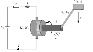
Consider a electromechanical system [57] shown in Fig. 1,

Refer to caption — Figure 1: Schematic of the electromechanical system.

whose dynamics is described as

\displaystyle\begin{cases}M\ddot{q}+B\dot{q}+N\sin(q)=I,\\ L\dot{I}+K_{B}\dot{q}+RI=V_{\varepsilon},\end{cases}

(47)

where $q(t)$ , $I(t)$ and $V_{\varepsilon}(t)$ are the angular motor position, the motor armature current, and the input control voltage, respectively, $M=\frac{J}{K_{\tau}}+\frac{m_{0}L_{0}^{2}}{3K_{\tau}}+\frac{M_{0}L_{0}^{2}}{K_{\tau}}+\frac{2M_{0}R_{0}^{2}}{5K_{\tau}}$ , $N=\frac{m_{0}L_{0}g}{2K_{\tau}}+\frac{M_{0}L_{0}g}{K_{\tau}}$ , $B=\frac{B_{0}}{K_{\tau}}$ , whose meanings and values of system symbols are shown in Table I.

TABLE I:

Symbol	Meaning	Value
$J$	the rotor inertia	$1.625\times 10^{-3}{\rm kg\cdot m^{2}}$
$m_{0}$	the link mass	$0.506{\rm kg}$
$M_{0}$	the load mass	$0.434{\rm kg}$
$L_{0}$	the link length	$0.305{\rm m}$
$R_{0}$	the radius of the load	$0.023{\rm m}$
$B_{0}$	the coefficient of viscous friction at the joint	$16.25\times 10^{-3}{\rm N\cdot m\cdot s/rad}$
$L$	the armature inductance	$15{\rm H}$
$R$	the armature resistance	$5.0{\rm\Omega}$
$K_{\tau}$	the electromechanical conversion coefficient of armature current to torque	$0.90{\rm N\cdot m/A}$
$K_{B}$	the back EMF coefficient	$0.90{\rm N\cdot m/A}$
$g$	the gravity coefficient	$9.81{\rm N/s^{2}}$

Let $x_{1}(t)=q(t),x_{2}(t)=\dot{q}(t),x_{3}(t)=\frac{I(t)}{M}$ and $u(t)=\frac{V_{\varepsilon}(t)}{ML}$ . Then, system (47) with mismatched uncertainties can be written as

\displaystyle\begin{cases}\dot{x}_{1}(t)=x_{2}(t)+\omega_{1}(t),\\ \dot{x}_{2}(t)=x_{3}(t)-\frac{N}{M}\sin(x_{1}(t))-\frac{B}{M}x_{2}(t)+\omega_{2}(t),\\ \dot{x}_{3}(t)=u(t)-\frac{K_{b}}{ML}x_{2}(t)-\frac{R}{ML}x_{3}(t)+\omega_{3}(t).\end{cases}

(48)

Therefore, it follows from Eq. (48), Assumptions Assumption 2 and Assumption 4 that one can choose $\underline{g_{i}}=0.1$ , $\bar{g}_{i}=10$ $(i=1,2,3)$ and $L_{1}=1$ , $L_{2}=\frac{N+B}{M}$ , $L_{3}=\frac{K_{B}+R}{ML}$ . In simulations, the disturbances $\omega_{1}(t)=2\sin(5t)$ , $\omega_{2}(t)=5\cos(2t)$ , $\omega_{3}(t)=10\sin(t)$ and the reference signal $y_{r}(t)=\sin(10t)+2$ .

Take $m=11$ and set the Gaussian membership functions as

\displaystyle\mu_{\Omega_{i}^{j}}(y_{r})=10{\rm e}^{-\frac{(y_{r}-\upsilon_{i}^{j})^{2}}{10}},

where $v_{i}=(v_{i}^{1},\cdots,v_{i}^{11})^{\top}=(-20,\cdots,-4,0,4,\cdots,20)^{\top}$ for $i=1,2,3$ . Moreover, control design parameters are selected as

	$\displaystyle b$	$\displaystyle=0.1,c=0.05,h=1,T=0.5,a=\frac{\frac{\pi}{2}-c}{{\rm e}^{-b}}=1.6807,$
	$\displaystyle\delta_{1}$	$\displaystyle=\sigma_{1}=10^{10},\delta_{i}=\sigma_{i}=\rho_{i}=\tau_{i}=10^{10}~{}(i=2,3),$
	$\displaystyle\varpi_{i}$	$\displaystyle=\mu_{i}=10~{}(i=1,2),\varrho_{i}=10,\lambda_{i}=10^{-5}~{}(i=2,3),$
	$\displaystyle\varpi_{3}$	$\displaystyle=5\times 10^{3},\mu_{3}=10,$

and two initial values are set as $\bar{x}_{3}^{1}(0)=(5,3,2)^{\top}$ and $\bar{x}_{3}^{2}(0)=-100\bar{x}_{3}^{1}(0)$ with $\hat{\theta}_{i}(0)=\mathbf{0}_{11}$ $(i=1,2,3)$ . Figs. 2 and 3 present the simulation results.

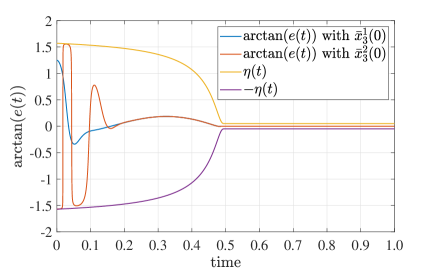
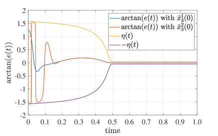
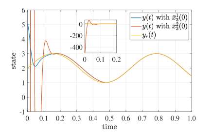
It can be observed from Figs. 2a and 3a that tracking error $e(t)$ always satisfies that $-\eta(t)<{\rm arctan}(e(t))<\eta(t)$ , equivalently, $\lvert e(t)\rvert<\tan(\eta(t))$ for any $t\geq 0$ , and $\lvert e(t)\rvert<\tan(0.05)$ for $t\geq 0.5$ . Therefore, the prescribed transient and steady state performances with prescribed time are achieved via proposed controllers. It should be emphasized that the state performances without approximating structures in Fig. 3 are almost identical to those with approximating structures in Fig. 2, but the computational complexity without approximating structures is far below the latter. The control mechanism without approximating structures can thus save more computation resources and have more potential to practical application.

In what follows, a single-link manipulator [58] shown in Fig. 4 is employed to compare the proposed controller without approximating structures and the one designed in [39].

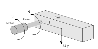
The single-link manipulator’s dynamics is

\displaystyle I\ddot{q}(t)+B\dot{q}(t)+Mgl\sin(q(t))=u(t),

(49)

where $g=9.81{\rm N/s^{2}}$ is the gravity coefficient, $q(t)$ is the angles of the link, $u(t)$ is the control input, $I$ is the total rotational inertias of the link and the motor, $l$ is the distance between the joint axis and the link center of mass, $M$ is the total mass of the single link, and $B$ is the damping coefficients. For simplicity, take $I=1{\rm kg\cdot m^{2}}$ , $B=2{\rm kg\cdot m/s}$ , $M=1{\rm kg}$ and $l=1{\rm m}$ .

Denote $x_{1}(t)=q(t)$ and $x_{2}(t)=\dot{q}(t)$ . Then, according to Eq. $(\ref{equ50})$ , the dynamics with external disturbance is

\displaystyle\begin{cases}\dot{x}_{1}(t)=x_{2}(t)+\omega_{1}(t),\\ \dot{x}_{2}(t)=-\frac{1}{I}(Bx_{2}(t)+Mgl\sin(x_{1}(t)))+\frac{1}{I}u(t)+\omega_{2}(t).\end{cases}

Let the reference signal $y_{r}(t)=\pi+2\sin(10t)$ , and disturbances $\omega_{1}(t)=0,\omega_{2}(t)=10\cos(5t)$ . In this example, take $\underline{g}_{1}=\underline{g}_{2}=0.5,$ $\bar{g}_{1}=\bar{g}_{2}=10$ , $L_{1}=1,L_{2}=\frac{B+Mgl}{I}$ , $\delta_{1}=\delta_{2}=\sigma_{1}=\sigma_{2}=\rho_{2}=\tau_{2}=10^{6}$ , $\varpi_{2}=\varrho_{2}=10$ and $\lambda_{2}=0.001$ . The parameters in prescribed performance functions are chosen as $b=0.9,c=0.05,T=0.5,h=1$ and $a=4.1340$ . In addition, Gaussian membership functions are the same as above. All initial values are chosen as zero. For the purpose of rigour in simulation, the settling time $t_{r}$ and initial value of prescribed performance function $\eta(0)$ in [39] are set as $t_{r}=T$ and $\eta(0)=\lvert e(0)\rvert+1$ , and the other parameters are the same as those in [39]. Therefore, $\psi=\frac{\eta_{0}^{\ell}}{\ell t_{r}}=16.1466$ , where $\ell=\frac{2}{13},\eta_{0}=\eta(0)-\eta_{t_{r}}$ and $\eta_{t_{r}}=\tan(c)$ . For convergence, denote the proposed controller and the one in [39] by $u_{1}(t)$ and $u_{2}(t)$ , respectively. The simulation results are displayed in Figs. 5, 6, 7 and 8.

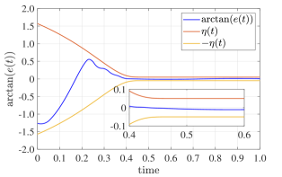
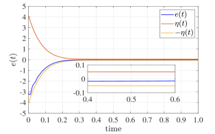
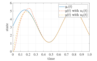
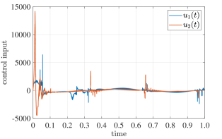
As shown in Figs. 5, 6 and 7, both controllers $u_{1}(t)$ and $u_{2}(t)$ can guarantee the prescribed transient and steady state performance of the tracking error within prescribed time, which again verifies the validity of Theorem Theorem 2. In addition, it can be seen from Fig. 8 that the absolute value of the proposed controller $u_{1}(t)$ with prescribed-time prescribed performance is generally less than controller $u_{2}(t)$ with finite-time prescribed performance, which demonstrates the effectiveness and practicality of the proposed methods.

V Conclusion

In this paper, the adaptive fuzzy tracking control with global prescribed-time prescribed performance for strict-feedback nonlinear systems with mismatched uncertainties has been investigated. Firstly, a class of prescribed-time prescribed performance functions independent of initial values and an error transformation function are designed. Secondly, two adaptive fuzzy controllers with and without approximating structures are designed to guarantee prescribed-time prescribed performance of the tracking error and the global uniform boundedness of all closed-loop signals. With a novel Lyapunov-like energy function, the differential explosion problem frequently occurring in backstepping techniques is solved. It is worth noting that no Nussbaum-type functions are used and no singular phenomenon occurs in the control design, and thus complex calculations can be avoided. Finally, some practical examples are employed to demonstrate the validity and effectiveness of the proposed methods. In future studies, the focus will be on the leader-following consensus with prescribed-time prescribed performance for strict-feedback multi-agent systems owing to their broad applications in various fields.

Acknowledgments

This work is supported by the National Natural Science Foundation of China under Grants 61973241 and 62176127.

References

[1] X. Wu, B. Mao, X. Wu and J. Lü, “Dynamic event-triggered leader-follower consensus control for multiagent systems,” SIAM Journal on Control and Optimization, vol. 60, no. 1, pp. 189–209, Jan. 2022.
[2] Y. Salmanpour, M. Mehdi Arefi, A. Khayatian and O. Kaynak, “Event-triggered fuzzy adaptive leader-following tracking control of nonaffine multiagent systems with finite-time output constraint and input saturation,” IEEE Transactions on Fuzzy Systems, vol. 30, no. 4, pp. 933–944, Apr. 2022.
[3] Y. Cai, H. Zhang, Y. Wang, Z. Gao and Q. He, “Adaptive bipartite fixed-time time-varying output formation-containment tracking of heterogeneous linear multiagent systems,” IEEE Transactions on Neural Networks and Learning Systems, vol. 33, no. 9, pp. 4688–4698, Sept. 2022.
[4] Y. Lu, X. Dong, Q. Li, J. Lü and Z. Ren, “Time-varying group formation-containment tracking control for general linear multiagent systems with unknown inputs,” IEEE Transactions on Cybernetics, vol. 52, no. 10, pp. 11055–11067, Oct. 2022.
[5] C. Liu, X. Wu and B. Mao, “Formation tracking of second-order multi-agent systems with multiple leaders based on sampled data,” IEEE Transactions on Circuits and Systems II: Express Briefs, vol. 68, no. 1, pp. 331–335, Jan. 2021.
[6] H. Liang, X. Guo, Y. Pan and T. Huang, “Event-triggered fuzzy bipartite tracking control for network systems based on distributed reduced-order observers,” IEEE Transactions on Fuzzy Systems, vol. 29, no. 6, pp. 1601–1614, Jun. 2021.
[7] G. Liu, M. V. Basin, H. Liang and Q. Zhou, “Adaptive bipartite tracking control of nonlinear multiagent systems with input quantization,” IEEE Transactions on Cybernetics, vol. 52, no. 3, pp. 1891–1901, Mar. 2022.
[8] A. Sen, S. R. Sahoo and M. Kothari, “Distributed average tracking with incomplete measurement under a weight-unbalanced digraph,” IEEE Transactions on Automatic Control, early access, May 31, 2022. [Online]. Available: https://doi.org/10.1109/TAC.2022.3179219.
[9] Y. Zhao, C. Xian, G. Wen, P. Huang and W. Ren, “Design of distributed event-triggered average tracking algorithms for homogeneous and heterogeneous multiagent systems,” IEEE Transactions on Automatic Control, vol. 67, no. 3, pp. 1269–1284, Mar. 2022.
[10] Y. Xu, X. Wu, B. Mao, J. Lü and C. Xie, “Fixed-time synchronization in the $p$ th moment for time-varying delay stochastic multilayer networks,” IEEE Transactions on Systems, Man, and Cybernetics: Systems, vol. 52, no. 2, pp. 1135–1144, Feb. 2022.
[11] Y. Xu, X. Wu, N. Li, J. Lu and C. Li, “Synchronization of complex networks with continuous or discontinuous controllers based on new fixed-time stability theorem,” IEEE Transactions on Systems, Man, and Cybernetics: Systems, early access, Otc. 13, 2022. [Online]. Available: https://ersp.lib.whu.edu.cn/s/org/doi/G.https/10.1109/TSMC.2022.3211621.
[12] N. Li, X. Wu, J. Feng, Y. Xu and J. Lü, “Fixed-time synchronization of coupled neural networks with discontinuous activation and mismatched parameters,” IEEE Transactions on Neural Networks and Learning Systems, vol. 32, no. 6, pp. 2470–2482, Jun. 2021.
[13] C. P. Bechlioulis and G. A. Rovithakis, “Robust adaptive control of feedback linearizable MIMO nonlinear systems with prescribed performance,” IEEE Transactions on Automatic Control, vol. 53, no. 9, pp. 2090–2099, Oct. 2008.
[14] C. P. Bechlioulis and G. A. Rovithakis, “Prescribed performance adaptive control for multi-input multi-output affine in the control nonlinear systems,” IEEE Transactions on Automatic Control, vol. 55, no. 5, pp. 1220–1226, May 2010.
[15] A. K. Kostarigka and G. A. Rovithakis, “Adaptive dynamic output feedback neural network control of uncertain MIMO nonlinear systems with prescribed performance,” IEEE Transactions on Neural Networks and Learning Systems, vol. 23, no. 1, pp. 138–149, Jan. 2012.
[16] A. Theodorakopoulos and G. A. Rovithakis, “A simplified adaptive neural network prescribed performance controller for uncertain MIMO feedback linearizable systems,” IEEE Transactions on Neural Networks and Learning Systems, vol. 26, no. 3, pp. 589–600, Mar. 2015.
[17] W. Shi, “Adaptive fuzzy output-feedback control for nonaffine MIMO nonlinear systems with prescribed performance,” IEEE Transactions on Fuzzy Systems, vol. 29, no. 5, pp. 1107–1120, May 2021.
[18] S. Gao, M. Li, Y. Zheng and H. Dong, “Expansive errors-based fuzzy adaptive prescribed performance control by residual approximation,” IEEE Transactions on Fuzzy Systems, vol. 30, no. 7, pp. 2736–2746, Jul. 2022.
[19] K. Zhao, Y. Song, C. L. P. Chen and L. Chen, “Adaptive asymptotic tracking with global performance for nonlinear systems with unknown Control directions,” IEEE Transactions on Automatic Control, vol. 67, no. 3, pp. 1566–1573, Mar. 2022.
[20] J. Zhang and G. Yang, “Prescribed performance fault-tolerant control of uncertain nonlinear systems with unknown control directions,” IEEE Transactions on Automatic Control, vol. 62, no. 12, pp. 6529–6535, Dec. 2017.
[21] F. Li and Y. Liu, “Control design with prescribed performance for nonlinear systems with unknown control directions and nonparametric uncertainties,” IEEE Transactions on Automatic Control, vol. 63, no. 10, pp. 3573–3580, Oct. 2018.
[22] J. Zhang, Q. Wang and W. Ding, “Global output-feedback prescribed performance control of nonlinear systems with unknown virtual control coefficients,” IEEE Transactions on Automatic Control, early access, Dec. 21, 2021. [Online]. Available: https://doi.org/10.1109/TAC.2021.3137103.
[23] J. Zhang and G. Yang, “Low-complexity tracking control of strict-feedback systems with unknown control directions,” IEEE Transactions on Automatic Control, vol. 64, no. 12, pp. 5175–5182, Dec. 2019.
[24] M. Lü, Z. Chen, B. De Schutter and S. Baldi, “Prescribed-performance tracking for high-power nonlinear dynamics with time-varying unknown control coefficients,” Automatica, vol. 146, p. 110584, Dec. 2022.
[25] L. Zhang and G. Yang, “Adaptive fuzzy prescribed performance control of nonlinear systems with hysteretic actuator nonlinearity and faults,” IEEE Transactions on Systems, Man, and Cybernetics: Systems, vol. 48, no. 12, pp. 2349–2358, Dec. 2018.
[26] W. Wang, D. Wang, Z. Peng and T. Li, “Prescribed performance consensus of uncertain nonlinear strict-feedback systems with unknown control directions,” IEEE Transactions on Systems, Man, and Cybernetics: Systems, vol. 46, no. 9, pp. 1279–1286, Sept. 2016.
[27] C. P. Bechlioulis and G. A. Rovithakis, “Decentralized robust synchronization of unknown high order nonlinear multi-agent systems with prescribed transient and steady state performance,” IEEE Transactions on Automatic Control, vol. 62, no. 1, pp. 123-134, Jan. 2017.
[28] I. Katsoukis and G. A. Rovithakis, “A low complexity robust output synchronization protocol with prescribed performance for high-order heterogeneous uncertain MIMO nonlinear multiagent systems,” IEEE Transactions on Automatic Control, vol. 67, no. 6, pp. 3128-3133, Jun. 2022.
[29] J. Qiu, K. Sun, T. Wang and H. Gao, “Observer-based fuzzy adaptive event-triggered control for pure-feedback nonlinear systems with prescribed performance,” IEEE Transactions on Fuzzy Systems, vol. 27, no. 11, pp. 2152–2162, Nov. 2019
[30] H. Dong, S. Gao, B. Ning, T. Tang, Y. Li and K. P. Valavanis, “Error-driven nonlinear feedback design for fuzzy adaptive dynamic surface control of nonlinear systems with prescribed tracking performance,” IEEE Transactions on Systems, Man, and Cybernetics: Systems, vol. 50, no. 3, pp. 1013–1023, Mar. 2020.
[31] G. S. Kanakis and G. A. Rovithakis, “Guaranteeing global asymptotic stability and prescribed transient and steady-state attributes via uniting control,” IEEE Transactions on Automatic Control, vol. 65, no. 5, pp. 1956-1968, May 2020.
[32] Y. Li, X. Shao and S. Tong, “Adaptive fuzzy prescribed performance control of nontriangular structure nonlinear systems,” IEEE Transactions on Fuzzy Systems, vol. 28, no. 10, pp. 2416–2426, Oct. 2020.
[33] F. Fotiadis and G. A. Rovithakis, “Prescribed performance control for discontinuous output reference tracking,” IEEE Transactions on Automatic Control, vol. 66, no. 9, pp. 4409–4416, Sept. 2021.
[34] L. N. Bikas and G. A. Rovithakis, “Prescribed performance tracking of uncertain MIMO nonlinear systems in the presence of delays,” IEEE Transactions on Automatic Control, early access, Dec. 14, 20211. [Online]. Available: https://doi.org/10.1109/TAC.2021.3135276.
[35] Y. Liu, X. Liu and Y. Jing, “Adaptive neural networks finite-time tracking control for non-strict feedback systems via prescribed performance,” Information Sciences, vol. 468, pp. 29–46, Nov. 2018.
[36] Y. Liu, X. Liu, Y. Jing and Z. Zhang, “A novel finite-time adaptive fuzzy tracking control scheme for nonstrict feedback systems,” IEEE Transactions on Fuzzy Systems, vol. 27, no. 4, pp. 646–658, Apr. 2019.
[37] S. Sui and S. Tong, “Finite-time fuzzy adaptive PPC for nonstrict-feedback nonlinear MIMO systems,” IEEE Transactions on Cybernetics, early access, Apr. 25, 2022. [Online]. Available: https://doi.org/10.1109/TCYB.2022.3163739.
[38] T. Jiang, J. Huang and X. Su, “Multivariable finite-time composite neural control via prescribed performance for error norm,” IEEE Transactions on Systems, Man, and Cybernetics: Systems, early access, Aug. 29, 2022. [Online]. Available: https://doi.org/10.1109/TSMC.2022.3199266.
[39] J. Qiu, T. Wang, K. Sun, I. J. Rudas and H. Gao, “Disturbance observer-based adaptive fuzzy control for strict-feedback nonlinear systems with finite-time prescribed performance,” IEEE Transactions on Fuzzy Systems, vol. 30, no. 4, pp. 1175–1184, Apr. 2022.
[40] S. Sui, C. L. P. Chen and S. Tong, “A novel adaptive NN prescribed performance control for stochastic nonlinear systems,” IEEE Transactions on Neural Networks and Learning Systems, vol. 32, no. 7, pp. 3196–3205, Jul. 2021.
[41] K. Sun, J. Qiu, H. R. Karimi and Y. Fu, “Event-triggered robust fuzzy adaptive finite-time control of nonlinear systems with prescribed performance,” IEEE Transactions on Fuzzy Systems, vol. 29, no. 6, pp. 1460–1471, Jun. 2021.
[42] H. Zhou, S. Sui and S. Tong, “Finite-time adaptive fuzzy prescribed performance formation control for high-order nonlinear multi-agent systems based on event-triggered mechanism,” IEEE Transactions on Fuzzy Systems, early access, Aug. 10, 2022. [Online]. Available: https://doi.org/10.1109/TFUZZ.2022.3197938.
[43] C. Zhu, C. Yang, Y. Jiang and H. Zhang, “Fixed-time fuzzy control of uncertain robots with guaranteed transient performance,” IEEE Transactions on Fuzzy Systems, early access, Jul. 27, 2022. [Online]. Available: https://doi.org/10.1109/TFUZZ.2022.3194373.
[44] F. Shojaei, M. M. Arefi, A. Khayatian and H. R. Karimi, “Observer-based fuzzy adaptive dynamic surface control of uncertain nonstrict feedback systems with unknown control direction and unknown dead-zone,” IEEE Transactions on Systems, Man, and Cybernetics: Systems, vol. 49, no. 11, pp. 2340–2351, Nov. 2019.
[45] K. Zhao, Y. Song, T. Ma and L. He, “Prescribed performance control of uncertain Euler-Lagrange systems subject to full-state constraints,” IEEE Transactions on Neural Networks and Learning Systems, vol. 29, no. 8, pp. 3478–3489, Aug. 2018.
[46] K. Zhao, Y. Song and L. Chen, “Tracking control of nonlinear systems with improved performance via transformational approach,” International Journal of Robust and Nonlinear Control, vol. 29, no. 6, pp. 1789–1806, Apr. 2019.
[47] Z. Shao, Y. Wang and X. Chen, “Global prescribed performance control for strict feedback systems pursuing uncertain target,” IEEE Transactions on Neural Networks and Learning Systems, early access, Jul. 25, 2022. [Online]. Available: https://doi.org/10.1109/TNNLS.2022.3189951.
[48] Y. Cao, J. Cao and Y. Song, “Practical prescribed time tracking control over infinite time interval involving mismatched uncertainties and non-vanishing disturbances,” Automatica, vol. 136, p. 110050, Feb. 2022.
[49] Y. Cao and Y. Song, “Performance guaranteed consensus tracking control of nonlinear multiagent systems: A finite-time function-based approach,” IEEE Transactions on Neural Networks and Learning Systems, vol. 32, no. 4, pp. 1536–1546, Apr. 2021.
[50] L. Wang and J. M. Mendel, “Fuzzy basis functions, universal approximation, and orthogonal least-squares learning,” IEEE Transactions on Neural Networks, vol. 3, no. 5, pp. 807-814, Sept. 1992.
[51] B. Cui, Y. Xia, K. Liu and G. Shen, “Finite-time tracking control for a class of uncertain strict-feedback nonlinear systems with state constraints: A smooth control approach,” IEEE Transactions on Neural Networks and Learning Systems, vol. 31, no. 11, pp. 4920–4932, Nov. 2020.
[52] M. Cai, P. Shi and J. Yu, “Adaptive neural finite-time control of non-strict feedback nonlinear systems with non-symmetrical dead-zone,” IEEE Transactions on Neural Networks and Learning Systems, early access, Jun. 09, 2022. [Online]. Available: https://doi.org/10.1109/TNNLS.2022.3178366.
[53] M. Krstic, I. Kanellakopoulos, and P. V. Kokotovic, Nonlinear and Adaptive Control Design (Adaptive and Learning Systems for Signal Processing, Communications and Control Series). Hoboken, NJ, USA: Wiley, 1995.
[54] Z. Ma and H. Ma, “Adaptive fuzzy backstepping dynamic surface control of strict-feedback fractional-order uncertain nonlinear systems,” IEEE Transactions on Fuzzy Systems, vol. 28, no. 1, pp. 122–133, Jan. 2020.
[55] C. Deng and G. Yang, “Distributed adaptive fuzzy control for nonlinear multiagent systems under directed graphs,” IEEE Transactions on Fuzzy Systems, vol. 26, no. 3, pp. 1356–1366, Jun. 2018.
[56] S. S. Ge and Cong Wang, “Adaptive neural control of uncertain MIMO nonlinear systems,” IEEE Transactions on Neural Networks, vol. 15, no. 3, pp. 674–692, May 2004.
[57] Y. Li, S. Tong, Y. Liu and T. Li, “Adaptive fuzzy robust output feedback control of nonlinear systems with unknown dead zones based on a small-gain approach,” IEEE Transactions on Fuzzy Systems, vol. 22, no. 1, pp. 164–176, Feb. 2014.
[58] B. Mao, X. Wu, J. Lü and G. Chen, “Predefined-time bounded consensus of multiagent systems with unknown nonlinearity via distributed adaptive fuzzy control,” IEEE Transactions on Cybernetics, early access, Apr. 15, 2022. [Online]. Available: https://doi.org/10.1109/TCYB.2022.3163755.

Hui Liu (S’11-M’14) received the B.S. and Ph.D. degrees in computational mathematics from Wuhan University, China, in 2005 and 2010 respectively. And she also received the Ph.D. degree in the field of systems and control from the University of Groningen, the Netherlands, in 2013. She is currently an associate professor with the School of Artificial Intelligence and Automation, Huazhong University of Science and Technology, Wuhan, China. She held visiting positions with the Academy of Mathematics and Systems Science, Chinese Academy of Sciences, Beijing, China, and with the Department of Electronic and Information Engineering, the Hong Kong Polytechnic University, Hong Kong. Her main research interests are in complex networks, cooperative control of networked systems, and intelligent control systems.