Adaptive finite element approximation of sparse optimal control with integral fractional Laplacian
Fangyuan Wang
School of Mathematics and Statistics, Shandong Normal University, Jinan, 250014, China
, Qiming Wang
School of Mathematical Sciences, Beijing Normal University, Zhuhai, 519087, China
and Zhaojie Zhou∗School of Mathematics and Statistics, Shandong Normal University, Jinan, 250014, China
In this paper we present and analyze a weighted residual a posteriori error estimate for an optimal control problem. The problem involves a nondifferentiable cost functional, a state equation with an integral fractional Laplacian, and control constraints. We employ subdifferentiation in the context of nondifferentiable convex analysis to obtain first-order optimality conditions. Piecewise linear polynomials are utilized to approximate the solutions of the state and adjoint equations. The control variable is discretized using the variational discretization method. Upper and lower bounds for the a posteriori error estimate of the finite element approximation of the optimal control problem are derived.
In the region where , the residuals do not satisfy the regularity. To address this issue, an additional weight is included in the weighted residual estimator, which is based on a power of the distance from the mesh skeleton.
Furthermore, we propose an h-adaptive algorithm driven by the posterior view error estimator, utilizing the Drfler labeling criterion. The convergence analysis results show that the approximation sequence generated by the adaptive algorithm converges at the optimal algebraic rate. Finally, numerical experiments are conducted to validate the theoretical results.
In this paper, we present and analyze a weighted residual a posteriori error estimate for an optimal control problem involving a nondifferentiable cost functional, a state equation with an integral fractional Laplacian, and control constraints. For a bounded Lipschitz domain , we consider
(1.1)
subject to
(1.2)
and the control constraints
Here parameters and . In the sequel,
is state and is the control variable. The function is referred to as desired state. To focus on the scenario of nondifferentiability, it is assumed that satisfy the condition that . We notice that the set , is a nonempty, bounded, closed and convex subset of .
The introduction of nonsmooth regularization term in the PDE-constrained optimization problems promotes sparsity in the solutions. This allows the control variable in the optimization process to tend towards zero in regions where it has negligible impact on the cost function, therefore minimizing the cost function. Sparse optimization is widely used in many practical applications, especially in the processing and analysis of high dimensional data, such as noise processing, machine learning, face recognition, etc.
Previous research has addressed the analysis of optimal control problems with a cost term containing norm [1, 2, 3, 4, 5, 6, 7, 8, 20]. For instance, in [7], the authors investigated the control problem constrained by a linear elliptic PDE, where the objective functional incorporated a regularization technique based on the control cost term. The authors analyzed the optimality conditions and proposed a semismooth Newton method that achieves local convergence with superlinear speed. Building upon this work, [8] provided a priori and posteriori error estimates through finite element analysis. Furthermore, in [5], the authors considered a semilinear elliptic PDE as the state equation and analyzed second-order optimality conditions. Additionally, the authors in [6] studied the sparse control problem with a fractional diffusion equation as the state equation. They analyzed a priori error estimate for the fully discrete case using finite element methods. More recently, Otrola et al. studied a sparse optimal control problem with a non-differentiable cost functional, where the state equations are Poisson’s problem and fractional diffusion equation, respectively in [9, 10]. In [9], the authors studied three different strategies for approximating the control variable, they proposed and analyzed a reliable and efficient a posteriori error estimate, and designed an adaptive strategy to achieve optimal convergence rates. In [10], the authors investigated an adaptive finite element method for sparse optimal control of fractional diffusion, taking into account the spectral definition of the fractional Laplacian operator.
In comparison to the priori error analysis of finite element approximations for PDE-constrained optimization, the design and analysis of a posteriori error estimate is not much. The initial work on reliable a posteriori error estimation for optimal control problems was presented in [11], followed by a series of related studies [12, 13, 14, 15, 16]. Residual-based a posteriori error estimates incorporating data oscillation were introduced in [17]. Later, a unified framework for the a posterior error analysis of linear quadratic optimal control problems with control constraints was established in [18], and the pure convergence of an adaptive finite element method for optimal control problems with variable divergence control was proved, that is, convergence without convergence rate. In [19], the authors rigorously proved convergence and quasi-optimality of AFEM for optimal control problem involving state and adjoint state variable.
However, to the best of our knowledge, no previous research has combined adaptive finite element methods (AFEMs) with integral fractional Laplacian sparse optimal control to address such problems. Therefore, in this paper, we focus on the adaptive finite element approximation for sparse optimal control with the integral fractional Laplacian. We outline and analyze the solution methodology for problem (1.1)-(1.2) based on the following considerations:
The optimal control problem involving the fractional Laplacian operator can effectively simulate groundwater pollution [21], turbulent flow [22], and chaotic dynamics [23]. Unlike integer-order diffusion equations, the fractional Laplacian operator exhibits power-law decay, which accurately captures heavy-tailed power-law decay phenomena observed in these applications. Hence, studying fractional optimal control problem is essential.
Objective functional by introducing the norm to control some specific physical quantities or locations, and the norm to maintain smoothness and continuity, can better solve the practical problems that need to control the optimal cost. The existence of term in the objective function
requires us to derive the first-order condition using a subdifferential approach [5, 7, 8], which is different from distributed optimal control problems.
Due to the non-locality, non-differentiability, and intrinsic constraints of the fractional Laplacian operator, by adopting adaptive strategies and a posteriori error estimate, we can identify singularities and refine the mesh accordingly, which can more effectively allocate computational resources and achieve higher accuracy with lower computational costs. One of the challenges in designing the a posterior error estimator is the nature of the residual, that is, it is not necessarily in . We refer to [26] and introduce the weighted residual estimator, where the weights are given by the power of the distance to the grid skeleton
(see section 4).
The adaptive finite element method is widely used, but there are not many convergence analyses of the algorithm. The optimal control problem we studied is a coupled system with nonlinear properties, which leads to the lack of orthogonality presented in [30] and brings difficulties to our convergence analysis. In order to address this issue, we refer to reference [28] and prove its quasi-orthogonality.
Recently, the only work on a posteriori error analysis for sparse optimal control constrained by fractional order equations, as in (1.1)-(1.2), is found in [10]. Compared with [10], this paper studies the integral definition of the fractional Laplacian operator, which plays an important role in the modeling of complex non-local and nonlinear phenomena such as diffusion, heat transfer, resistance and elasticity. And the main difference is that the convergence of the adaptive algorithm is also analyzed in this paper. In this paper, we use piecewise linear polynomial dispersion for the state variable and variational discretization for the control variable. We design a posterior error estimator that requires only discretization of the state variable and adjoint variable. Notably, in the , the residual does not satisfy the -regularity. To address this issue, an additional weight based on the power of the distance from the mesh skeleton is included in the weighted residual estimator. An h-adaptive algorithm driven by the Drfler marking criterion based on the a posteriori error estimator is proposed and its convergence is proved.
The organization of the paper is as follows: In section 2, we introduce the symbols used and provide a brief overview of elements in convex analysis, along with the regularity of solutions to optimal control problem. In section 3, we analyze the first-order optimality conditions for the problem. In section 4, we introduce the finite element discretization of the optimal control problem (1.1)-(1.2) and design a weighted residual estimator. The core of our work is presented in sections 4 and 5. For the discretization introduced at the beginning of section 4, we first derive upper and lower bounds for the a posteriori error estimate of the finite element approximation for the optimal control problem. An h-adaptive algorithm driven by the posterior view error estimator based on Drfler labeling criterion is proposed. In section 5, we show that the sequence of approximations produced by the adaptive algorithm converges at the optimal algebraic rate. In section 6, a series of numerical examples are provided to demonstrate the effectiveness of our theoretical findings.
2. Preliminaries
In this section we introduce some preliminaries about fractional Sobolev spaces, subdifferential and fractional Laplacian.
For a bounded domain denotes the Banach spaces of standard 2-th Lebesgue integrable functions on . For denotes the fractional Sobolev space. is the subspace of consisting of functions whose trace is zero on . Let and denote the inner product and norm in , respectively. The
seminorm and the full norm are denoted as follows
Moreover, we introduce the following space, which will be used in the weak formulation of state equation
Next, we will review some concepts with respect to subdifferentials from convex analysis that will be useful in our upcoming analysis. For details, please refer to [24].
Consider a real and normed vector space . Suppose be a convex and proper functional. Let be such that . A subgradient of at is an element that satisfies
(2.1)
Here, represents the duality pairing between and . The set of all subgradients of at , denoted by , refers to the subdifferential of at .
As is a convex functional, the subdifferential at any point within the effective domain of is not empty. Additionally, it is important to note that the subdifferential is monotone, i.e.,
(2.2)
Finally, we introduce the definition of fractional Laplacian:
(2.3)
Here , and
and ”p.v.” denotes the principal value of the integral:
(2.4)
where is a ball of radius centered at . The difference in the numerator of (2.3), which vanishes at the singularity, provides a regularization, which together with averaging of positive and negative parts allows the principal value to exist.
A consequence of this definition is the mapping property (see [25]).
3. Optimal control problem
The weak formulation of state equation (1.2) reads: Find such that
(3.1)
Here
We define
As the seminorm is equivalent to the norm on (see [29]), by Lax-Milgram theorem, the solution exists and is unique.
For the state equation with the right hand we can define a linear and bounded solution operator such that .
Moreover, the following regularity result holds for the state equation.
Here , for and for as well as a constant depending on and .
The weak formulation of the optimal control problem (1.1)-(1.2) reads:
(3.2)
subject to
(3.3)
Since the is strictly convex and weakly lower semicontinuous, this problem admits a unique optimal solution .
In order to obtain optimality conditions for (3.2)-(3.3), we introduce the following adjoint state as follows:
(3.4)
Set
and . Then we obtain the reduced problem of (1.1):
(3.5)
Although the reduced cost functional (3.5) is nonsmooth, it consists in the sum of a regular part and a convex nondifferentiable term. Thanks to the structure, optimality conditions can still be established according to the following result.
Lemma 3.2.
([27])
Let be defined as in (3.5). The element is a minimizer of over if and only if there exists a subgradient such that
(3.6)
Theorem 3.1.
(Optimality conditions)
If is an optimal solution to (3.5), then it satisfies the following variational inequality
These three properties are equivalent to (3.10). Therefore, (3.9), (3.10), (3.12) the previous estimate allow us to deduce (3.11)
which completes the proof.
∎
At end we present the following first order optimality conditions for above optimal control problems.
Theorem 3.3.
Let be the solution of the optimal control problem (3.2)-(3.3). Then there exists an adjoint state , such that
(3.13)
4. Finite element approximation method and a posteriori error estimate
We begin by partitioning the domain into simplices with size , forming a conforming partition . We then define and denote by the collection of conforming and shape regular meshes that are refinements of an initial mesh .
For let be the finite element space consisting of continuous piecewise linear functions over the triangulation
For all elements and , we introduce the -th order element patch inductively by
The finite element approximation of the optimal control problem (3.2)-(3.3) can be characterized as
subject to
(4.1)
Here the admissible set of control is not discretized, i.e., the so-called
variational discretization approach.
Similar to the continuous case we have the discrete first order optimality condition
(4.2)
where
Next, we give the following discrete projection formula.
Lemma 4.1.
Suppose are the optimal variables associated to (4.2), then we obtain
(4.3)
(4.4)
(4.5)
Similar to the continuous case, we can define a discrete control-to-state mapping .
Set Then we have for with
Lemma 4.2.
Assume that and are the solutions of the continuous and discretised state equation with right hand term . Then the following error estimates hold
and
Proof.
We invoke the Galerkin orthogonality to arrive at
Thus we have
Next, let be the solution of the following problem with
Then we have
Setting , to prove the second estimate, we invoke the Galerkin orthogonality and the previous estimate to arrive at
Consequently,
∎
To derive a posteriori error analysis we need to introduce the following auxiliary problems
(4.6)
Note that the residuals do not satisfy the -regularity for . To address this issue, we require a weight function to measure the distance from the mesh skeleton. For a mesh , we introduce the weight function defined in [26]
We further define the corresponding weighted residual errors as follows
(4.7)
(4.8)
where
Then on a subset , we define the error estimators of the state and adjoint state by
Thus, and constitute the error estimators for the state equation
and the adjoint state equation on with respect to as follows
Moreover we also need the Scott-Zhang operator([26]) that satisfy the following properties
(4.9)
(4.10)
(4.11)
Lemma 4.3.
For , and the weighted residual error estimator is reliable:
Moreover, for and , the estimator is also efficient
Proof.
Note that and are finite element approximations of and . We refer the reader to [26] for details on the proof of the upper and lower bounds in the Lemma.
∎
We define
(4.12)
(4.13)
Here . can be described similarly by
(4.14)
Due to the variational
approach is considered, we have that Thus a posteriori error indicators and estimators for the optimal control variable and the associated subgradient are zero, i.e.,
(4.15)
In the subsequent analysis, let represent a generic constant with distinct values in different instances.
We define the errors the vector , and the norm
(4.16)
4.1. Reliability of the error estimator
Theorem 4.1.
Let and be the solutions of problems (3.13) and (4.2), respectively. Then the following upper bound of a posteriori error holds for
Here
(4.17)
Proof.
We proceed in five steps.
By applying the triangle inequality and Lemma 4.3, we can readily obtain
(4.18)
Moreover, by the coercivity of the bilinear form , we can derive
Since the control variable is implicitly discretized, the error estimators with respect to and are zeros. By (4.29) and (4.30) we can derive
the estimate only for state and adjoint state
Here .
4.2. Efficiency of the error estimator
Theorem 4.2.
Suppose that and are the solutions of the optimal control problem of (3.13) and (4.2), respectively. If , for some parameter then we have the error estimator , defined as in (4.17) satisfied the following lower bound for
We can deal with the second term of (4.32) in a similar way
where denotes the maximum times of an element appearing in all element patch .
On the basis of (4.32) and the previous estimate, we immediately obtain the local efficiency of
Assuming that the initial size of the mesh fulfills the following condition: For , we can obtain
(4.35)
Note that
We need to estimate using the dual argument in the following analysis.
Let be the solution of the following problem
In an analogous way we obtain
Then we can get
(4.36)
Using the previous inequality, we can obtain
and
Thus we have
(4.37)
Combining the estimate (4.35) and (4.37) we derive
This concludes the proof.
∎
5. AFEMs and convergence analysis
The optimal control , due to the sparsity term in the cost functional, is sparse and has sparsely support sets within .
The fractional Laplacian operator is nonlocal ([32, 33, 34]) and can lead to singularity of the state variable and the adjoint variable near the boundary ([35]), which leads to a lower convergence rate ([36, 37]).
To overcome these hurdle, adaptive mesh refinement methods can be employed. The method facilitate more comprehensive mesh refinement in areas where the solution singularity is intense, and consequently improving the numerical solution’s accuracy.
5.1. AFEMs
Utilizing the residual error estimator to measure local contributions, we explore an established technique for adaptive mesh refinement known as , which employs Drfler’s marking criterion to designate elements for refinement.
: Initial mesh with mesh size , constraints and , regularization parameter , sparsity parameter . Set and solve (4.2) to obtain
: Given a parameter ; Construct a minimal subset such that
: We bisect all the elements that are contained in
with the newest-vertex bisection method and create a new mesh
. Refine
Algorithm 1Design of the AFEMs:
In the first step of , we used the following projection gradient algorithm:
Start with the mesh with mesh size .
Given the initial value , and a tolerance
.
Solving the state equation in (4.2) to get state variable ;
Solving the adjoint state equation in (4.2) to obtain adjoint state variable ;
Using (4.5) to compute the associted subgradient and control variable
Calculate the error:
Update the control variable
Algorithm 2Projection gradient algorithm
5.2. Convergence analysis
To establish the quasi-optimality of Adaptive Finite Element Methods (AFEMs), we employ the framework proposed by Carstensen et al. in [28]. The fulfillment of several prerequisites is necessary to establish quasi-optimality in adaptive algorithms: (1) Stability, (2) Reduction, (3) Discrete reliability and (4) Quasi-orthogonality. The stability prerequisite ensures the stability of error estimate on non-refined elements, while the reduction prerequisite guarantees a reduction in error on refined elements. The discrete reliability ensures the ability of the error estimators on refined elements to effectively control the error between coarse and fine grid solutions. The quasi-orthogonality prerequisite involves providing a measure for the relationship between the error estimators and the exact errors. These requirements will be rigorously validated through a series of mathematical proofs.
Theorem 5.1.
(Stability)
We use to denote the refinements of . For any subsets , there holds
where the constant .
Proof.
From the definition of (4.7), (4.8) and (4.31) we can obtain
where Note that
and
By the Lipschitz continuity of the operator , we have that
An application of
and
yields
Further by the inverse estimate for fractional Laplacian ([26]) we have
This result allows us to derive that
∎
Theorem 5.2.
(Reduction) We use to denote the refinements of . Then we have
where the constant , for for Here and
Proof.
Bisection ensures that for any and its descendants with Note that
(5.1)
we prove the Theorem with Here denotes the bisection time of every element in the refinement.
By the definition of (4.7), the relationship between and we can get
(5.2)
Similarly,
Then we have
Therefore, the previous estimate allows us to deduce the reduction property on the refined elements
Similar arguments can be applied to . Using the definition of (4.17), we can thus arrive at the estimate
(5.6)
Lemma 5.1.
Set and . Then the following estimates hold
Proof.
By the coercivity and Galerkin orthogonality we derive
Assume We obtained by applying (4.9) and (4.11) in the above estimation
which yields the first result. The second result can be derived in an analogous way.
∎
Theorem 5.3.
(Discrete reliability)
We use to denote the refinements of . There holds
Proof.
Taking and as the continuous solutions and and as its approximation, respectively. It can be deduced from
the coercivity of , Galerkin orthogonality and Lemma 5.1 that
Similar arguments can be applied to bound . Using the previous inequality, we can thus arrive at the estimate
Combining the above estimates yields
∎
The optimal control system is a coupled system with nonlinear characteristics. These nonlinear characteristics lead to a lack of support for orthogonality when attempting to prove a contraction. Therefore, we need to prove quasi-orthogonality next.
Let be the solution associated to the discrete problem (4.1) with respect to and be the solution associated to the discrete problem (4.1) with respect to . We assume is a refinement of , and define the following norm
(5.7)
and
(5.8)
where is the optimal solution of the problem (3.2)-(3.3). Then the following relation is satisfied
(5.9)
Theorem 5.4.
(Quasi-orthogonality) By the above definitions, there holds
Here, , for all the constant is depend
on and the -shape regularity of the initial triangulation .
Proof.
At first we prove the case For convenience, we use to denote and . So it suffices to proceed in five steps.
Since , we have that
(5.10)
To control the right hand side of (5.2), we utilize the auxiliary state , defined as , the control defined in (3.13) and combine (4.28), Lemma 4.2 to obtain
The goal of this step is to bound . Similarly, Since , we have that
In an analogous way, we utilize the auxiliary adjoint state , defined as , the control defined in (3.13) and combine (4.29), Lemma 4.2, (4.2) to obtain
By the relation (5.9) and Lemma 5.1, combining above estimates leads to
Further, a simple application of the triangle inequality reveal that
To conclude the previous estimate combined with Theorem 4.1 and Remark 5.1 leads to the general quasi-orthogonality as follows
This concludes the proof.
∎
For each , if there exists constants such that
(5.11)
we say that the adaptive Algorithm 2 is rate optimal with respect to the
error estimator, where
According to [28], through the proof of the above Theorem we indeed also verify that Algorithm 1 can reach the optimal convergence order in the sense of (5.11).
6. Numerical results
In this section, three numerical experiments are presented, and the exact solutions in the circle domain of the first example are given. The solutions in the square domain of the second and third examples are not known. We proceed by establishing fixed values for the optimal state and adjoint state variable, by employing the projection formulas
and
.
Example 6.1.
We set , , , and the exact solutions are as follows:
Figure 6.1 shows the initial mesh and the final refinement mesh with . Since the exact solutions of the state variable and adjoint variable exhibit smoothdness within the unit circle, with singularities on the boundary, so the mesh is refined mainly in the region close to the boundary.
Figure 6.1. The initial mesh (left) and the final refinement mesh (right) with on the circle.
In Figure 6.2, the computational rates of convergence for the computable error estimators and indicators and for and are presented, respectively. It can be observed that, in both cases, each contribution decays with the optimal rate .
Figure 6.2. The convergent behaviors of the indicators and estimators for (left) and (right).
We set and the parameter that governs the module . The left plot of Figure 6.3 illustrates the convergence orders of the error estimators and error indicators under different values of . On the right plot of Figure 6.3, the convergence orders of the errors for the state and adjoint variables in and the effectivity indices which are given by are presented for different values. From the Figure 6.3, it is observed that when , indicating uniform refinement, the displayed convergence rates do not reach optimality. However, for the convergence rates of the error eatimators and errors clearly converge to . Thus, our theoretical analysis is effectively verified.
Figure 6.3. The convergent behaviors of the errors, indicators and estimators for fixed and respectively on the circle.
Next, we consider the effect of changing the regularization parameter on the system with and . Specifically, we examine the cases where takes the values of
It can be seen from the Figure 6.4 that the error estimators , the error indicators errors of state and adjoint variable in can reach the optimal convergence order for all the values of the parameter considered.
Figure 6.4. The convergent behaviors of the errors, indicators and estimators for all the values of the parameter respectively on the circle.
In Figures 6.5-6.6, we show the profiles of the numerical solutions for the control and state when , respectively. It can be seen that as decreases, the term dominates and the numerical solutions of the control become sparsier.
Figure 6.5. The profiles of the numerically computed control with (a), (b), and (c).
Figure 6.6. The profiles of the numerically computed state with (a), (b), and (c).
Example 6.2.
In the second example we consider an optimal control problem with . We set , , , , , respectively.
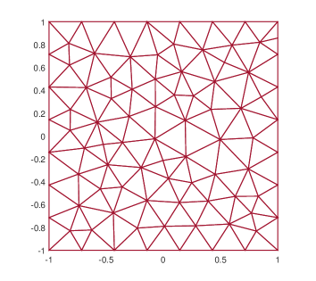
In Figure 6.7 we show the initial mesh and the final refinement mesh with . The primary refinement behavior is observed to occur exclusively along the boundaries of the entire square domain. This observation suggests that the estimators effectively capture the singularities of the exact solution along the entire boundary, thus guiding the mesh refinement process.
Figure 6.7. The initial mesh (left) and the final refinement mesh (right) with on the square.
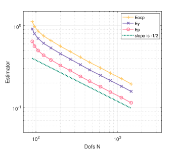
For and , the Figure 6.8 shows that the AFEM proposed in Section 6 delivers
optimal experimental rates of convergence for the error estimators , the error indicators The results obtained empirically are consistent with those of the previous example. The convergence rates of the estimators and indicators are for uniform refinement, while adaptive refinement leads to optimal convergence rates of .
Figure 6.8. The convergent behaviors of the indicators and estimators for (left) and (right).
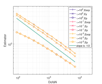
For all choices of the parameter considered, the Figure 6.9 shows the decrease of the total error estimators and the error indicators with respect to the number of degrees of freedom (Dofs). In all the values of the parameter cases the optimal rate is achieved.
Figure 6.9. The convergent behaviors of the indicators and estimators for all the values of the parameter respectively on the square. We have considered (left), (right)
In Figures 6.10-6.11, we show the profiles of the numerical solutions for the control when and , respectively. As decreases, the numerical solutions of the control become sparsier.
Figure 6.10. The profiles of the numerically computed control with (a), (b) and (c).
Figure 6.11. The profiles of the numerically computed control with (a), (b) and (c).
Example 6.3.
In the third example we consider an optimal control problem with . We set , , , , , respectively.
In Figure 6.12 we show the initial mesh and the refinement mesh after 13 adaptive steps with . We observe that the mesh nodes are distributed around the domain where the solutions have a large gradient as well as at the boundarys. In Figure 6.13, the convergence rates of error estimators and indicators for and are presented, respectively. It can be observed that, in both cases, each contribution decays with the optimal convergence rate . In Figure 6.14, the profiles of the numerical control and state with are provided.
Figure 6.12. The initial mesh (left) and the final refinement mesh (right) with on the square.
Figure 6.13. The convergent behaviors of the indicators and estimators for (left) and (right).
Figure 6.14. The numerical control(left) and state (right) with .
7. Conclusion
In this paper, we present and analyze a weighted residual a posteriori error estimate for an optimal control problem. The problem involves a cost functional that is nondifferentiable, a state equation with an integral fractional Laplacian, and control constraints. We provide first-order optimality conditions and derive upper and lower bounds on the a posteriori error estimates for the finite element approximation of the optimal control problem. Moreover, we demonstrate that the approximation sequence generated by the adaptive algorithm converges at the optimal algebraic rate. Finally, we validate the theoretical findings through numerical experiments.
Acknowledgements
The work was supported by the National Natural
Science Foundation of China under Grant No. 11971276 and 12171287.
References
[1] Clason, C., Kunisch, K.: A duality-based approach to ellipic control problems in nonreflexive Banach spaces. ESAIM Control Optim. Calc. Var. 17, 243-266 (2011)
[2] Casas, E., Herzog, R., Wachsmuth, G.: Approximation of sparse controls in semilinear equations by piecewise linear functions, Numer. Math. 122,
645-669 (2012)
[3] Casas, E.: A review on sparse solutions in optimal control of partial differential equations. SeMA Journal, 74, 319-344 (2017)
[4] Casas, E. and Kunisch, K.: Stabilization by sparse controls for a class of semilinear parabolic equations. SIAM J. Control Optim., 55, 512-532 (2017)
[5] Casas, E., Herzog, R., Wachsmuth, G.: Optimality conditions and error analysis of semilinear elliptic control problems with cost functional. SIAM J. Optim., 22, 795-820 (2012)
[6] Otrola, E., Salgado, A.J.: Sparse optimal control for fractional diffffusion. Comput. Methods Appl. Math., 18(1), 95-110 (2018)
[7]Stadler, G.: Elliptic optimal control problems with -control cost and applications for the placement of control devices. Comput. Optim. Appl., 44, 159-181 (2009)
[8] Wachsmuth, G., Wachsmuth, D.: Convergence and regularization results for optimal control problems with sparsity functional. ESAIM Control Optim. Calc. Var., 17, 858-866 (2011)
[9] Allendes, A., Fuica, F., Otrola, E.: Adaptive finite element methods for sparse PDE-constrained optimization. IMA J. Numer. Anal., 40(3), 2106-2142 (2020)
[10] Otrola, E.: An adaptive finite element method for the sparse optimal control of fractional diffusion. Numer. Meth. Part. D. E., 36(2), 302-328 (2019)
[11] Liu, W.B., Yan, N.N.: A posteriori error analysis for convex distributed
optimal control problems. Adv. Comput. Math. 15(1-4), 285-309 (2001)
[12] Liu, W.B., Yan, N.N.: A posteriori error estimates for convex boundary
control problems. SIAM J. Numer. Anal. 39(1), 73-99 (2001)
[13] Li, R., Liu, W.B., Ma, H.P., Tang, T.: Adaptive finite element approximation for distributed elliptic optimal control problems. SIAM J. Control
Optim. 41(5), 1321-1349 (2002)
[14] Liu, W.B., Yan, N.N.: A posteriori error estimates for optimal problems governed by Stokes equations. SIAM J. Numer. Anal. 40, 1850-1869
(2003)
[15] Liu, W.B., Yan, N.N.: A posteriori error estimates for optimal control
problems governed by parabolic equations. Numer. Math. 93, 497-521
(2003)
[16] Liu, W.B., Yan, N.N.: Adaptive Finite Element Methods for Optimal
Control Governed by PDEs. Science Press, Beijing (2008)
[17] Hintermller, M., Hoppe, R.H.W.: Goal-oriented adaptivity in control
constrained optimal control of partial differential equations. SIAM J.
Control Optim. 47(4), 1721-1743 (2008)
[18] Kohls, K., Rsch, A., Siebert, K.G.: A posteriori error analysis of optimal
control problems with control constraints. SIAM J. Control Optim. 52,
1832-1861 (2014)
[19] Gong, W., Yan, N.N.: Adaptive finite element method for elliptic optimal
control problems: convergence and optimality. Numer. Math. 135, 1121-1170 (2017)
[20] Leng, H.T., Chen, Y.P., Huang, Y.Q.: Equivalent a posteriori error estimates for elliptic optimal control problems with -control cost, Comput. Math. Appl. 77(2), 342-356 (2019)
[21] Benson, D.A., Wheatcraft, S., Meerschaert. M.: The fractional-order governing equation of Lévy motion. Water Resour. Res., 36(6), 1413-1424, 2000.
[25] Bonito, A., Borthagaray, J.P., Nochetto, R.H., Otrola, E., Salgado, A.J.: Numerical
methods for fractional diffusion, Comput. Vis. Sci. 19, 19-46 (2018)
[26] Faustmann, M., Melenk, J.M., Praetorius, D.: Quasi-optimal convergence
rate for an adaptive method for the integral fractional Laplacian. Math. Comp. 90(330), 1557-1587 (2021)
[27] Ioffe, A.D., Tichomirov, V.M.: Theorie der Extremalaufgaben. VEB Deutscher Verlag der Wissenschaften, Berlin (1979).
[28] Carstensen, C., Feischl, M., Praetorius, D.: Axioms of adaptivity. Comput.
Math. Appl. 67(6), 1195-1253 (2014)
[29] Acosta, G., Borthagaray, J.P.: A fractional laplace equation: regularity of solutions and finite element approximations. SIAM J. Numer. Anal., 55(2), 472-495 (2017)
[30] Cascon, J.M., Kreuzer, C., Nochetto, R.H., Siebert, K.G.: Quasi-optimal convergence rate for an adaptive finite element method, SIAM J. Numer. Anal. 46,
2524-2550 (2008)
[31] Borthagaray, J.P., Leykekhman, D., Nochetto, R.H.: Local energy estimates for the fractional Laplacian. SIAM J. Numer. Anal. 59(4), 1918-1947 (2021)
[32] Cabr, X., Tan, J.: Positive solutions of nonlinear problems involving the square root of the Laplacian. Adv. Math., 224(5), 2052-2093 (2010)
[33] Caffarelli L., Silvestre, L.: An extension problem related to the fractional Laplacian. Comm. Part. Diff. Eqs., 32(7-9), 1245-1260 (2007)
[34] Caffarelli, L.A., Stinga, P.R.: Fractional elliptic equations, Caccioppoli estimates and regularity. Ann. Inst. H. Poincar Anal. Non Linaire, 33(3), 767-807 (2016)
[35] Capella, A., Dvila, J., Dupaigne, L., Sire, Y.: Regularity of radial extremal solutions for some non-local semilinear equations. Comm. Part. Diff. Eqs., 36(8), 1353-1384 (2011)
[36] Banjai, L., Melenk, J.M., Nochetto, R.H., Otrola, E., Salgado, A.J., Schwab. Ch.: Tensor FEM
for spectral fractional diffusion. Found. Comput. Math., 19, 901-962 (2019)
[37] Nochetto, R.H., Otrola, E., Salgado, A.J.: A PDE approach to fractional diffusion in general domains: a priori error analysis. Found. Comput. Math., 15(3), 733-791 (2015)