Adaptive Central-Upwind Scheme on Triangular Grids for the Saint-Venant System

Yekaterina Epshteyn¹¹¹1Department of Mathematics, The University of Utah, Salt Lake City, UT 84112, USA; epshteyn@math.utah.edu and Thuong Nguyen²²2Department of Mathematics, The University of Utah, Salt Lake City, UT 84112, USA; tnguyen@math.utah.edu

Abstract

In this work we develop a robust adaptive well-balanced and positivity-preserving central-upwind scheme on unstructured triangular grids for shallow water equations. The numerical method is an extension of the scheme from [Liu et al.,J. of Comp. Phys, 374 (2018), pp. 213 - 236]. As a part of the adaptive central-upwind algorithm, we obtain local a posteriori error estimator for the efficient mesh refinement strategy. The accuracy, high-resolution and efficiency of new adaptive central-upwind scheme are demonstrated on a number of challenging tests for shallow water models.

keywords:

Saint-Venant system of shallow water equations, central-upwind scheme, well-balanced and positivity-preserving scheme, adaptive algorithm, weak local residual error estimator, unstructured triangular grid

AMS subject classification: 76M12, 65M08, 35L65, 86-08, 86A05

1 Introduction

We consider the two-dimensional (2-D) Saint-Venant system of shallow water equations,


	$\displaystyle h_{t}+(hu)_{x}+(hv)_{y}=0,$		(1.1a)
	$\displaystyle(hu)_{t}+\Big{(}hu^{2}+\frac{g}{2}h^{2}\Big{)}_{x}+(huv)_{y}=-ghB_{x},$		(1.1b)
	$\displaystyle(hv)_{t}+(huv)_{x}+\Big{(}hv^{2}+\frac{g}{2}h^{2}\Big{)}_{y}=-ghB_{y},$		(1.1c)

where $t$ is the time, $x$ and $y$ are horizontal spatial coordinates ( $(x,y)\in\Omega$ ), $h(x,y,t)$ is the water height, $u(x,y,t)$ and $v(x,y,t)$ are the $x$ - and $y$ -components of the flow velocity, $B(x,y)$ is the bottom topography, and $g$ is the constant gravitational acceleration. The system (1.1a)–(1.1c) was originally proposed in [12], but it is still widely used to model water flow in rivers, lakes and coastal areas, to name a few examples. The Saint-Venant system (1.1a)–(1.1c) is an example of the hyperbolic system of balance/conservation laws. The design of robust and accurate numerical algorithms for the computation of its solutions is important and challenging problem that has been extensively studied in the recent years.

An accurate numerical scheme for shallow water equations (1.1a)–(1.1c) should preserve the physical properties of the flow. For example, i) the numerical method should be positivity preserving, that is, the water height $h$ should be nonnegative at all times. The positivity preserving property ensures a robust performance of the algorithm on dry ( $h$ is zero) or almost dry ( $h$ is near zero) states; ii) in addition, the numerical method for system (1.1a)–(1.1c) should be well-balanced, the method should exactly preserve the “lake-at-rest” solution, $h+B\equiv const,u\equiv 0,v\equiv 0.$ This property diminishes the appearance of unphysical oscillations of magnitude proportional to the grid size. In the past decade, several well-balanced [15, 16, 4, 1, 17, 22, 23, 25, 30, 7, 33, 34, 39, 40, 41, 42, 46, 47, 16, 35, 18, 2, 6, 5, 36] and positivity preserving [1, 25, 30, 40, 35, 8, 4, 2, 6, 5, 36] schemes (non exhaustive lists) for shallow water models have been proposed, but only few satisfy both major properties i) and ii) simultaneously.

The traditional numerical methods for system (1.1a)–(1.1c) consider very fine fixed meshes to reconstruct delicate features of the solution. However, this can lead to high computational cost, as well as to a poor accuracy of small scale characteristics of the problem. Therefore, the main goal of this work is to design adaptive numerical algorithm for shallow water equations. In this work, we extend numerical method in [36] to adaptive well-balanced and positivity-preserving central-upwind finite volume method on unstructured triangular grids. The central Nessyahu-Tadmor schemes, their generalization into higher resolution central schemes and semidiscrete central-upwind schemes are a family of efficient and accurate Godunov-type Riemann problem-free projection-evolution finite volume methods for hyperbolic problems. They were originally developed in [38, 31, 28]. The main advantages of these numerical algorithms are the high-resolution, efficiency and their simplicity. The class of central-upwind methods has been successfully used for problems in science and engineering, including, for geophysical flow problems and related models, e.g. [31, 32, 28, 25, 7, 30, 10, 9, 11, 27, 26, 3, 29, 5, 6, 44, 36]. There is some very recent effort on the design of adaptive well-balanced and positivity-preserving central-upwind schemes on quad-tree grids for shallow water models [43, 19], but no research has been done for the development of such adaptive schemes on unstructured triangular grids.

This paper is organized as follows. In Section 2, we briefly review well-balanced positivity-preserving central-upwind scheme on unstructured triangular grids [36] which serves as the underlying discretization for the developed adaptive algorithm. We give summary of the adaptive central-upwind method in Section 3.1. We discuss adaptive mesh refinement strategy in Section 3.2. In Section 3.3, we present adaptive second-order strong stability preserving Runge-Kutta method, employed as a part of time evolution for the adaptive central-upwind scheme. We derive local a posteriori error estimator in Section 3.4 which is used as a robust indicator for the adaptive mesh refinement in our work. Finally, in Section 4, we illustrate the high accuracy and efficiency of the developed adaptive central-upwind scheme on a number of challenging tests for shallow water models.

2 Semi-Discrete Central-Upwind Scheme – an Overview

In this work, we employ the central-upwind scheme discussed in this section as the underlying discretization for the developed adaptive central-upwind algorithm, Section 3. Therefore, in this section, we will briefly review a semi-discrete second-order well-balanced positivity preserving central-upwind scheme on unstructured triangular grids for the Saint-Venant system of shallow water equations [6, 36].

In the first work [6], a new second-order semi-discrete central-upwind scheme was developed for computing the solutions of the system (1.1a)–(1.1c) on unstructured triangular grids. The key ideas in the development of the scheme in [6] were: 1) Change of variables from $(h,hu,hv)^{T}$ to variables $(w:=h+B,hu,hv)^{T}$ . This change of variables simplifies the construction of the well-balanced scheme since in the “lake-at-rest” steady-state, it is the equilibrium variable, the water surface $w\equiv h+B$ (but not the conservative variable, the water height $h$ ) that has to stay constant; 2) Replacement of the bottom topography function $B$ with its continuous piecewise linear approximation; 3) Design of the special positivity preserving correction of the piecewise linear reconstruction for the water surface $w$ ; 4) Development of a special well-balanced finite-volume-type quadrature for the discretization of the cell averages of the geometric source term. The developed scheme in [6], enforced the positivity of the water height $h$ , and preserved the “lake-at-rest” steady state in the case of fully submerged bottom topography. In the recent work [36], we further improved the well-balanced property of the scheme from [6], and extended the scheme to accurate and stable simulations of shallow water models with dry or near dry states (e.g., waves arriving or leaving the shore). We will briefly review below the central-upwind scheme from [36].

First, we rewrite the system (1.1a)–(1.1c) in the following equivalent form,

\bm{U}_{t}+\bm{F}(\bm{U},B)_{x}+\bm{G}(\bm{U},B)_{y}=\bm{S}(\bm{U},B),

(2.1)

where the variables $\bm{U}$ and the fluxes $\bm{F}$ and $\bm{G}$ are

\bm{U}=\left(\begin{array}[]{c}w\\[7.74998pt] hu\\[7.74998pt] hv\end{array}\right),\quad\bm{F}=\left(\begin{array}[]{c}hu\\ \dfrac{(hu)^{2}}{w-B}+\dfrac{g}{2}(w-B)^{2}\\[6.45831pt] \dfrac{(hu)(hv)}{w-B}\end{array}\right),\quad\bm{G}=\left(\begin{array}[]{c}hv\\ \dfrac{(hu)(hv)}{w-B}\\[6.45831pt] \dfrac{(hv)^{2}}{w-B}+\dfrac{g}{2}(w-B)^{2}\end{array}\right),

and the source term $\bm{S}$ is

\bm{S}=\left(\begin{array}[]{c}0\\ -g(w-B)B_{x}\\[2.15277pt] -g(w-B)B_{y}\end{array}\right).

Refer to caption — Figure 2.1: A typical triangular cell with three neighbors.

As illustrated in Figure 2.1, we denote,

${\mathcal{T}}:=\bigcup_{j}T_{j}$ is an unstructured triangulation of the computational domain $\Omega$ ;

$T_{j}\in\mathcal{T}$ is a triangular cell of size $|T_{j}|$ with the barycenter $(x_{j},y_{j})$ ;

$V_{j\kappa}=(\widetilde{x}_{j\kappa},\widetilde{y}_{j\kappa}),~{}\kappa=12,23,31$ are the three vertices of $T_{j}$ ;

$T_{jk},~{}k=1,2,3$ are the neighboring triangles that share a common side with $T_{j}$ ;

$\ell_{jk}$ is the length of the common side of $T_{j}$ and $T_{jk}$ , and $M_{jk}$ is its midpoint;

$\bm{n}_{jk}:=(\cos(\theta_{jk}),\sin(\theta_{jk}))^{\top}$ is the outer unit normal to the $k$ th side of $T_{j}$ .

Next, in order to develop the positivity-preserving and well-balanced scheme, the bottom topography $B$ is replaced with its continuous piecewise linear approximation $\widetilde{B}$ given by

\left|\begin{array}[]{ccc}x-\widetilde{x}_{j12}&y-\widetilde{y}_{j12}&{\widetilde{B}}(x,y)-\widehat{B}_{j12}\\[2.15277pt] \widetilde{x}_{j23}-\widetilde{x}_{j12}&\widetilde{y}_{j23}-\widetilde{y}_{j12}&\widehat{B}_{j23}-\widehat{B}_{j12}\\[2.15277pt] \widetilde{x}_{j13}-\widetilde{x}_{j12}&\widetilde{y}_{j13}-\widetilde{y}_{j12}&\widehat{B}_{j13}-\widehat{B}_{j12}\end{array}\right|=0,\quad(x,y)\in T_{j},

where, in the case of continuous bottom topography, $\widehat{B}_{j\kappa}:=B(V_{j\kappa})~{}\kappa=12,23,31$ . Then, denote:

B_{jk}:=\widetilde{B}(M_{jk}),\quad B_{j}:=\widetilde{B}(x_{j},y_{j})=\frac{1}{3}(\widehat{B}_{j12}+\widehat{B}_{j23}+\widehat{B}_{j13}).

At time $t$ , define by $\hbox{\vbox{\hrule height=0.5pt\kern 1.72218pt\hbox{\kern-0.50003pt$\bm{U}$\kern-0.50003pt}}}_{j}(t)$ the approximation of the cell averages of the solution,

\hbox{\vbox{\hrule height=0.5pt\kern 1.72218pt\hbox{\kern-0.50003pt$\bm{U}$\kern-0.50003pt}}}_{j}(t)\approx\frac{1}{|T_{j}|}\iint\limits_{T_{j}}\bm{U}(x,y,t)\,dxdy.

Then, it can be shown (see [36, 6]), that the semi-discrete second-order central-upwind scheme for the Saint-Venant system (2.1) on triangular grid is given by the following system of ODEs,

\displaystyle\frac{d\,\hbox{\vbox{\hrule height=0.5pt\kern 1.72218pt\hbox{\kern-0.50003pt$\bm{U}$\kern-0.50003pt}}}_{j}}{dt}=

\displaystyle-\frac{1}{|T_{j}|}\big{[}\bm{H}_{j1}+\bm{H}_{j2}+\bm{H}_{j3}\big{]}+\hbox{\vbox{\hrule height=0.5pt\kern 1.72218pt\hbox{\kern-0.50003pt$\bm{S}$\kern-0.50003pt}}}_{j},

(2.2)

where the numerical fluxes through the edges of the triangular cell $T_{j}$ are

$\displaystyle\bm{H}_{jk}=$	$\displaystyle\frac{\ell_{jk}\cos(\theta_{jk})}{a_{jk}^{\rm in}+a_{jk}^{\rm out}}\Big{[}{a_{jk}^{\rm in}\bm{F}(\bm{U}_{jk}(M_{jk}),B_{jk})+a_{jk}^{\rm out}\bm{F}(\bm{U}_{j}(M_{jk}),B_{jk})}\Big{]}$	(2.3)
$\displaystyle+$	$\displaystyle\frac{\ell_{jk}\sin(\theta_{jk})}{a_{jk}^{\rm in}+a_{jk}^{\rm out}}\Big{[}{a_{jk}^{\rm in}\bm{G}(\bm{U}_{jk}(M_{jk}),B_{jk})+a_{jk}^{\rm out}\bm{G}(\bm{U}_{j}(M_{jk}),B_{jk})}\Big{]}$
$\displaystyle-$	$\displaystyle\ell_{jk}\frac{a_{jk}^{\rm in}a_{jk}^{\rm out}}{a_{jk}^{\rm in}+a_{jk}^{\rm out}}\big{[}\bm{U}_{jk}(M_{jk})-\bm{U}_{j}(M_{jk})\big{]},\quad k=1,2,3.$

Here, $\bm{U}_{j}(M_{jk})$ and $\bm{U}_{jk}(M_{jk})$ are the reconstructed point values of $\bm{U}$ at the middle points of the edges $M_{jk}$ . To obtain these values [36], first, a piecewise linear reconstruction of the variables $\bm{\Upsilon}:=(w,u,v)^{\top}$ is computed as,

\widetilde{\bm{\Upsilon}}(x,y)=\sum\limits_{j}\bm{\Upsilon}_{j}(x,y){\Large{\mbox{$\chi$}}}_{T_{j}},\quad\bm{\Upsilon}_{j}(x,y):=\bm{\Upsilon}_{j}+(\widehat{\bm{\Upsilon}}_{x})_{j}(x-x_{j})+(\widehat{\bm{\Upsilon}}_{y})_{j}(y-y_{j}),

(2.4)

where ${\Large{\mbox{$\chi$}}}_{T_{j}}$ is the characteristic function of the cell $T_{j}$ , $\bm{\Upsilon}_{j}$ are the point values of $\bm{\Upsilon}$ at the cell centers and $(\widehat{\bm{\Upsilon}}_{x})_{j}$ and $(\widehat{\bm{\Upsilon}}_{y})_{j}$ are the limited partial derivative. After that, the second and third components of the point values $\bm{U}_{j}(M_{jk})$ and $\bm{U}_{jk}(M_{jk})$ are obtained from, $\bm{\Upsilon}_{j}(M_{jk})$ and $\bm{\Upsilon}_{jk}(M_{jk})$ ,

		$\displaystyle(hu)_{j}(M_{jk})=(w_{j}(M_{jk})-B_{jk})\,u_{j}(M_{jk}),$		$\displaystyle(hu)_{jk}(M_{jk})=(w_{jk}(M_{jk})-B_{jk})\,u_{jk}(M_{jk}),$
		$\displaystyle(hv)_{j}(M_{jk})=(w_{j}(M_{jk})-B_{jk})\,v_{j}(M_{jk}),$		$\displaystyle(hv)_{jk}(M_{jk})=(w_{jk}(M_{jk})-B_{jk})\,v_{jk}(M_{jk}).$

See Section 2 in [36] for more details on the reconstruction.

Moreover, to design a well-balanced central-upwind scheme, a special second-order reconstruction of water surface is introduced in [36] which is positivity preserving for the steady-state solutions with partially flooded/dry cells. Hence, the linear approximation for the water surface is updated as follows:

•

In the dry cells in which $\hbox{\vbox{\hrule height=0.5pt\kern 1.72218pt\hbox{\kern-0.50003pt$w$\kern-0.50003pt}}}_{j}=B_{j}$ , the corresponding linear pieces for $w$ in (2.4) are replaced by,

$\widetilde{w}_{j}(x,y)=\widetilde{B}(x,y).$ (2.5)

•

If $T_{j}$ is a partially flooded which means $B_{j}<\hbox{\vbox{\hrule height=0.5pt\kern 1.72218pt\hbox{\kern-0.50003pt$w$\kern-0.50003pt}}}_{j}<\max\{\widehat{B}_{j23},\widehat{B}_{j13},\widehat{B}_{j12}\}$ , the water surface is reconstructed by using two linear pieces instead of one as,

\widetilde{w}_{j}(x,y)=\begin{cases}\mathring{w}_{j}(x,y),\quad&\text{if}\quad(x,y)\in T^{wet}_{j},\\ \widetilde{B}(x,y),\quad&\text{otherwise},\end{cases}

(2.6)

where $\mathring{w}_{j}(x,y)$ is a linear reconstruction of the water surface on the wet part $T^{wet}_{j}$ of the cell $T_{j}$ .

•

If $T_{j}$ is a fully flooded $\hbox{\vbox{\hrule height=0.5pt\kern 1.72218pt\hbox{\kern-0.50003pt$w$\kern-0.50003pt}}}_{j}\geq\max\{\widehat{B}_{j23},\widehat{B}_{j13},\widehat{B}_{j12}\}$ , no further modification for the linear approximation (2.4) is needed.

See Section 3 in [36] for more details of the reconstruction of the water surface $w$ .

In (2.3), $a_{jk}^{\rm in}$ and $a_{jk}^{\rm out}$ are the one-sided local speeds of propagation in the directions $\pm\bm{n}_{jk}$ . These speeds are related to the largest and smallest eigenvalues of the Jacobian matrix $J_{jk}=\cos(\theta_{jk})\,\frac{\partial{\bm{F}}}{\partial{\bm{U}}}+\sin(\theta_{jk})\,\frac{\partial{\bm{G}}}{\partial{\bm{U}}}$ , denoted by $\lambda_{+}[J_{jk}]$ and $\lambda_{-}[J_{jk}]$ , respectively, and are defined by

		$\displaystyle a^{\rm in}_{jk}=-\min\{\lambda_{-}[J_{jk}(\bm{U}_{j}(M_{jk}))],\,\lambda_{-}[J_{jk}(\bm{U}_{jk}(M_{jk})],\,0\},$		(2.7)
		$\displaystyle a^{\rm out}_{jk}=\max\{\lambda_{+}[J_{jk}(\bm{U}_{j}(M_{jk}))],\,\lambda_{+}[J_{jk}(\bm{U}_{jk}(M_{jk})],\,0\},$		(2.7)

where

		$\displaystyle\lambda_{\pm}[J_{jk}(\bm{U}_{j}(M_{jk}))]=\cos(\theta_{jk})u_{j}(M_{jk})+\sin(\theta_{jk})v_{j}(M_{jk})\pm\sqrt{gh_{j}(M_{jk})},$
		$\displaystyle\lambda_{\pm}[J_{jk}(\bm{U}_{jk}(M_{jk}))]=\cos(\theta_{jk})u_{jk}(M_{jk})+\sin(\theta_{jk})v_{jk}(M_{jk})\pm\sqrt{gh_{jk}(M_{jk})}.$

Remark 2.1

In order to avoid division by 0 (or by a very small positive number), the numerical flux (2.3) is replaced with

	$\displaystyle\bm{H}_{jk}=$	$\displaystyle\frac{\ell_{jk}\cos(\theta_{jk})}{2}\left[\bm{F}(\bm{U}_{jk}(M_{jk}),B_{jk})+\bm{F}(\bm{U}_{j}(M_{jk}),B_{jk})\right]$
	$\displaystyle+$	$\displaystyle\frac{\ell_{jk}\sin(\theta_{jk})}{2}\left[\bm{G}(\bm{U}_{jk}(M_{jk}),B_{jk})+\bm{G}(\bm{U}_{j}(M_{jk}),B_{jk})\right]$

wherever $a_{jk}^{\rm in}+a_{jk}^{\rm out}<\sigma$ . In all of the reported numerical examples in Section 4, we have taken $\sigma=10^{-6}$ .

A fully discrete scheme can be obtained by numerically solving the ODE system (2.2), (2.3) using a stable and sufficiently accurate ODE solver. The time-step size on each cell $T_{j}\in\mathcal{T}$ should satisfy the CFL-type condition (see [6]), which can be expressed as,

\Delta t<\frac{1}{6}\min_{j,k}\left[\frac{r_{jk}}{\max(a^{\rm in}_{jk},a^{\rm out}_{jk})}\right],

(2.8)

where $r_{j1}$ , $r_{j2}$ and $r_{j3}$ are the three corresponding altitudes of the triangle $T_{j}$ . However, the condition (2.8) can become too restrictive on partially flooded cells. Thus, for partially flooded cells, the “draining” time-step technique is used to ensure the positivity of the scheme without reducing the time step size (2.8), [4, 36]. Namely, first the “draining” time-step $\Delta t_{j}^{\rm drain}$ is defined by,

\Delta t_{j}^{\rm drain}:=\frac{|T_{j}|\,\hbox{\vbox{\hrule height=0.5pt\kern 1.72218pt\hbox{\kern-0.50003pt$h$\kern-0.50003pt}}}_{j}^{\,n}}{\sum\limits_{k=1}^{3}\max(0,H^{(1)}_{jk})}

where $H^{(1)}_{jk}$ is the first component of the numerical flux ${\bm{H}}_{jk}$ given by (2.3). Notice that, for fully flooded cells $\Delta t_{j}^{\rm drain}=\Delta t$ , while for dry cells $\Delta t_{j}^{\rm drain}=0$ . Next, the local “draining” time-step $\Delta t_{jk}$ for each edge $k$ of the cell $T_{j}\in\mathcal{T}$ is defined as,

\Delta t_{jk}=\begin{cases}\min(\Delta t,\Delta t^{drain}_{j}),\quad\text{if}\quad H^{(1)}_{jk}>0,\\ \min(\Delta t,\Delta t^{drain}_{jk}),\quad\text{if}\quad H^{(1)}_{jk}\leq 0,\\ \end{cases}

(2.9)

where $\Delta t^{drain}_{jk}$ is the “draining” time-step in the neighboring triangle $T_{jk}\in\mathcal{T}$ of $T_{j}$ and $\Delta t$ is computed by (2.8), but with the minimum taken there over the flooded cells only. This procedure of the draining time step is a part of the adaptive SSPRK2 time evolution (3.5a)-(3.5b) in Section 3.3.

Finally, the cell average of the source term $\bm{S}_{j}$ in (2.2),

\hbox{\vbox{\hrule height=0.5pt\kern 1.72218pt\hbox{\kern-0.50003pt$\bm{S}$\kern-0.50003pt}}}_{j}(t)\approx\frac{1}{|T_{j}|}\iint\limits_{T_{j}}\bm{S}\big{(}\bm{U}(x,y,t),B(x,y)\big{)}\,dxdy,

has to be discretized in a well-balanced manner [36]:
Quadrature for $\hbox{\vbox{\hrule height=0.5pt\kern 1.72218pt\hbox{\kern-0.50003pt$S$\kern-0.50003pt}}}^{\,(2)}_{j}$ is

	$\displaystyle\hbox{\vbox{\hrule height=0.5pt\kern 1.72218pt\hbox{\kern-0.50003pt$S$\kern-0.50003pt}}}^{\,(2)}_{j}$	$\displaystyle=\frac{g}{2\|T_{j}\|}\sum_{k=1}^{3}\ell_{jk}\cos(\theta_{jk})\cdot\frac{\Delta t_{jk}}{\Delta t}\cdot\big{[}w(M_{jk})-B(M_{jk})\big{]}^{2}$		(2.10)
		$\displaystyle-\frac{g}{3}\Big{[}(w_{j12}-\widehat{B}_{j12})\,w_{x}(V_{j12})+(w_{j23}-\widehat{B}_{j23})\,w_{x}(V_{j23})+(w_{j13}-\widehat{B}_{j13})\,w_{x}(V_{j13})\Big{]}.$		(2.10)

A similar quadrature for $\hbox{\vbox{\hrule height=0.5pt\kern 1.72218pt\hbox{\kern-0.50003pt$S$\kern-0.50003pt}}}^{\,(3)}_{j}$ is

	$\displaystyle\hbox{\vbox{\hrule height=0.5pt\kern 1.72218pt\hbox{\kern-0.50003pt$S$\kern-0.50003pt}}}^{\,(3)}_{j}$	$\displaystyle=\frac{g}{2\|T_{j}\|}\sum_{k=1}^{3}\ell_{jk}\sin(\theta_{jk})\cdot\frac{\Delta t_{jk}}{\Delta t}\cdot\big{[}w(M_{jk})-B(M_{jk})\big{]}^{2}$		(2.11)
		$\displaystyle-\frac{g}{3}\Big{[}(w_{j12}-\widehat{B}_{j12})\,w_{y}(V_{j12})+(w_{j23}-\widehat{B}_{j23})\,w_{y}(V_{j23})+(w_{j13}-\widehat{B}_{j13})\,w_{y}(V_{j13})\Big{]}.$		(2.11)

Remark 2.2

Note, that in Section 4, we compare performance of the developed adaptive central-upwind scheme Section 3 with a performance of the central-upwind scheme without adaptivity from [36] (see also brief review above). We use standard SSPRK2 time discretization [20] together with the draining time step for the scheme without adaptivity from [36] in numerical experiments in Section 4.

3 Adaptive Central-Upwind Scheme

The traditional numerical schemes are based on the use of very fine fixed meshes to reconstruct delicate features of the solution. This can lead to high computational cost, as well as poor resolution of all small scale features of the problem. In many engineering and scientific applications, it is beneficial to use adaptive meshes for improving the accuracy of the approximation at a much lower cost. Therefore, in this section, we will introduce an efficient and accurate adaptive central-upwind algorithm.

3.1 Adaptive Central-Upwind Algorithm

The adaptive central-upwind algorithm is described briefly by the following steps.

Step 0. At time $t=t^{0}$ , generate the initial uniform grid $\mathcal{T}^{0,0}$ .

Step 1. On mesh $\mathcal{T}^{n,\mathcal{M}_{n}}$ , evolve the cell averages $\hbox{\vbox{\hrule height=0.5pt\kern 1.72218pt\hbox{\kern-0.50003pt$\bm{U}$\kern-0.50003pt}}}^{n}$ of the solution from time $t^{n}$ to $\hbox{\vbox{\hrule height=0.5pt\kern 1.72218pt\hbox{\kern-0.50003pt$\bm{U}$\kern-0.50003pt}}}^{n+1}$ at the next time level $t^{n+1}$ using adaptive central-upwind scheme (3.5a)-(3.5b), see Section 3:

•

At time $t^{n}$ , determine the level $l=0,1,...,L$ of each cell/triangle $T^{n,\mathcal{M}_{n}}_{j}\in\mathcal{T}^{n,\mathcal{M}_{n}}$ , (3.1), Section 3.3.
•

At each time level $t^{n,p}_{l},p=0,1,...,\mathcal{P}_{l}-1$ , perform the piecewise polynomial reconstruction (2.4) and compute the point values, Section 2, Section 3.3.
•

At each time level $t^{n,p}_{l},p=0,1,...,\mathcal{P}_{l}-1$ , calculate the one-sided local speeds of propagation using (2.7), Section 2, Section 3.3.
•

At time $t^{n}$ , calculate the reference time step $\Delta t$ using (3.3), Section 3.3.
•

At each time level $t^{n,p}_{l},p=0,1,...,\mathcal{P}_{l}-1$ , compute the local time step for each cell level, (3.4), Section 3.3.
•

At each time level $t^{n,p}_{l},p=0,1,...,\mathcal{P}_{l}-1$ , compute numerical fluxes and source term in the adaptive central-upwind scheme (3.5a)-(3.5b), (2.3), (2.10)-(2.11), Section 2, Section 3.3.

Step 2. On mesh $\mathcal{T}^{n,\mathcal{M}_{n}}$ , compute WLR error using (3.14) in Section 3.4 and update the refinement/de-refinement status for each cell/triangle, Section 3.4.

Step 3. Generate the new adaptive mesh $\mathcal{T}^{n+1,\mathcal{M}_{n+1}}$ at $t^{n+1}$ , Section 3.2. This step includes coarsening of some cells, refinement of some cells, and the appropriate projection of the cell averages from the mesh $\mathcal{T}^{n,\mathcal{M}_{n}}$ at $t^{n}$ onto a new adaptive mesh $\mathcal{T}^{n+1,\mathcal{M}_{n+1}}$ at time $t^{n+1}$ , Section 3.2.

Step 4. Repeat Step 1 - Step 3 until final time.

3.2 Adaptive Mesh Refinement/Coarsening

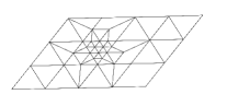
The main idea of the proposed adaptive mesh refinement algorithm is as follows. At time $t^{n}$ , we start with the given mesh, denoted as $\mathcal{T}^{n,m}=\{T^{n,m}_{j}\}$ , where $T^{n,m}_{j}$ is a triangular cell of size $|T^{n,m}_{j}|$ with the barycenter $(x^{n,m}_{j},y^{n,m}_{j})$ within the initial mesh $\mathcal{T}^{n,m}$ , and index $m=0,1,2...$ is the level of refinement ( $m=0$ corresponds to the mesh with no refinement and $\mathcal{T}^{n,0}\equiv\mathcal{T}^{0,0}$ for all $n$ ). To flag triangular cells in the mesh $\mathcal{T}^{n,m}$ for the refinement/de-refinement (or coarsening), we use weak local residual (WLR) error estimate, see Section 3.4. We apply “regular refinement” on the triangles flagged for refinement to obtain a new mesh $\mathcal{T}^{n,m+1}$ with the refinement level $m+1$ . The “regular refinement” on a fully flooded triangle is obtained by splitting each flagged triangle (“parent” triangle) into four smaller triangles (“children” triangles) by inserting a new node at the mid-point of each edge of the “parent” triangle. We illustrate this idea using Fig. 3.1 (a), where we show an example of splitting a flagged triangle $T^{n,m}_{j}$ by using the mid-points of the sides to obtain the “children” cells $T^{n,m+1}_{j_{s}},s=1,2,3,4$ . In addition, the insertion of new nodes on the edges means that non-flagged triangles adjacent to refined triangles get hanging nodes and must also be refined. This is done by inserting a new edge between the hanging node and the opposite corner as illustrated in Fig. 3.1 (b).

In practice, we may want to reach a higher level of refinement for some cells. This happens when those cells have very large WLR error (3.14), and we need to add more data points. We can obtain a finer cell by repeating the refinement for the flagged triangles in the refined mesh $\mathcal{T}^{n,m+1}$ to get the mesh with higher level $\mathcal{T}^{n,m+2},m=0,1,2,....$ . Fig. 3.2 is the illustration of the “regular refinement” procedure with two levels of refinement.

In the partially flooded cells, Section 2, the approximation of the water surface $\widetilde{w}(x,y)$ at each time level $t^{n}$ consists of two linear pieces, the piece for the wet and for the dry region, see Fig. 3.3. This motivates an idea of the “wet/dry refinement” which uses the boundary between the wet region and the dry region of the cell to refine the partially flooded triangles as shown in the example in Fig. 3.4 (left). Namely, consider a partially flooded triangle $T^{n,m}_{j}$ which is flagged for the refinement and has three non-flagged neighboring cells in the grid $\mathcal{T}^{n,m}$ . The segment $I_{1}I_{2}$ is the boundary between the wet and dry interface in that triangle. Note that, the location of the nodes $I_{1}$ and $I_{2}$ is determined by the second order water surface reconstruction developed in [36], see also Section 2. During “regular refinement” of the partially flooded cell, we first split the flagged cell $T^{n,m}_{j}$ into a smaller triangle and a quadrilateral using the wet/dry interface $I_{1}I_{2}$ . We then continue to refine the quadrilateral by its diagonal. As can be seen in Fig. 3.4 (left), the flagged triangle $T^{n,m}_{j}$ has three “children” which are either fully flooded or dry. Similarly, as in Fig. 3.1, the appearance of two hanging nodes $I_{1}$ and $I_{2}$ on two sides leads to the need of the further splitting of the neighboring cells as presented in Fig. 3.4 (right). The “regular wet/dry refinement” will capture the features of the wet/dry fronts and will minimize number of partially flooded “children” cells. However, this method may give us difficulties in controlling the shape of triangles in the adaptive mesh. In some cases, it may produce “children” cells with unexpected large obtuse angles or very small altitudes, as shown in Fig. 3.5. For cells where such situation happens, we instead use the “regular refinement” for the fully flooded cells as described above.

Very often in the numerical simulations of the wave phenomena, the regions of the domain that need to be refined move with time. Hence, the refinement in some cells may become no longer needed. The de-refinement or coarsening procedure is then introduced to deactivate unnecessarily fine cells in the mesh. The de-refinement is performed by coarsening (by deactivating “children” cells) in the triangles of the mesh flagged for coarsening (and possibly deactivating finer neighboring triangles due to removal of the hanging nodes). At time $t^{n}$ , “children” cells in the mesh $\mathcal{T}^{n,m+1},m=0,1,...,M_{n}-1$ , are deactivated based on the WLR and the corresponding “parent” cell from the mesh $\mathcal{T}^{n,m}$ is activated back. In order to minimize the complexity of the adaptive grid generation, the de-refinement should be applied on all cells flagged for coarsening prior to the refinement, see for example [21].

The refinement/de-refinement process at time $t^{n}$ produces a hierarchical system of grids $\mathcal{S}^{n}=\{\mathcal{T}^{n,0},\mathcal{T}^{n,1},\mathcal{T}^{n,2},...,\mathcal{T}^{n,\mathcal{M}_{n}}\}$ , where $\mathcal{T}^{n,m}$ , $m=1,2,...,\mathcal{M}_{n}$ is the grid with the level of refinement $m$ obtained by refining the grid $\mathcal{T}^{n,m-1}$ . The final mesh $\mathcal{T}^{n,\mathcal{M}_{n}}\in\mathcal{S}^{n}$ is the mesh that is used in the adaptive central-upwind scheme (3.5a)-(3.5b) at time level $t^{n}$ . After the evolution of the numerical solution from time $t^{n}$ to time $t^{n+1}$ using mesh $\mathcal{T}^{n,\mathcal{M}_{n}}\in\mathcal{S}^{n}$ , we proceed with the generation of a new adaptive grid $\mathcal{T}^{n+1,\mathcal{M}_{n+1}}\in\mathcal{S}^{n+1}$ from the mesh $\mathcal{T}^{n,\mathcal{M}_{n}}$ , using WLR in Section 3.4. After a new adaptive mesh $\mathcal{T}^{n+1,\mathcal{M}_{n+1}}$ is constructed, the obtained cell averages $\hbox{\vbox{\hrule height=0.5pt\kern 1.72218pt\hbox{\kern-0.50003pt$\bm{U}$\kern-0.50003pt}}}^{n+1}$ on the mesh $\mathcal{T}^{n,\mathcal{M}_{n}}$ need to be projected accurately on the new mesh $\mathcal{T}^{n+1,\mathcal{M}_{n+1}}$ , using the ideas as summarized briefly below.

Case 1. If a triangle $T^{n+1,\mathcal{M}_{n+1}}_{j}\in\mathcal{T}^{n+1,\mathcal{M}_{n+1}}$ at $t^{n+1}$ is the same cell as in the grid $\mathcal{T}^{n,\mathcal{M}_{n}}$ , we will keep without any change the cell averages for that triangle at $t^{n+1}$ .

Case 2. A cell $T^{n+1,\mathcal{M}_{n+1}}_{j}\in\mathcal{T}^{n+1,\mathcal{M}_{n+1}}$ is obtained by coarsening some finer cells $T^{n,\mathcal{M}_{n}}_{j_{s}}\in\mathcal{T}^{n,\mathcal{M}_{n}},s=1,2,..,S$ . In order to enforce the conservation, the solution, $\hbox{\vbox{\hrule height=0.5pt\kern 1.72218pt\hbox{\kern-0.50003pt$U$\kern-0.50003pt}}}^{n+1}_{j}$ in the cell $T^{n+1,\mathcal{M}_{n+1}}_{j}$ , is computed as

\displaystyle\hbox{\vbox{\hrule height=0.5pt\kern 1.72218pt\hbox{\kern-0.50003pt$U$\kern-0.50003pt}}}^{n+1}_{j}

\displaystyle=\dfrac{1}{|T^{n+1,\mathcal{M}_{n+1}}_{j}|}\sum\limits_{s=1}^{S}\hbox{\vbox{\hrule height=0.5pt\kern 1.72218pt\hbox{\kern-0.50003pt$U$\kern-0.50003pt}}}^{n}_{j_{s}}|T^{n,\mathcal{M}_{n}}_{j_{s}}|,

where $\hbox{\vbox{\hrule height=0.5pt\kern 1.72218pt\hbox{\kern-0.50003pt$U$\kern-0.50003pt}}}^{n}_{j_{s}}$ is the solution in $T^{n,\mathcal{M}_{n}}_{j_{s}}$ .

Case 3. A triangle $T^{n+1,\mathcal{M}_{n+1}}_{j}\in\mathcal{T}^{n+1,\mathcal{M}_{n+1}}$ is obtained from the refinement of the cell $T^{n,\mathcal{M}_{n}}_{i}\in\mathcal{T}^{n,\mathcal{M}_{n}}$ . The approximation of the cell averages of the solution at $t^{n+1}$ in $\mathcal{T}^{n+1,\mathcal{M}_{n+1}}$ is obtained using the evaluation of the piecewise linear reconstruction (2.4) of the solution at $t^{n+1}$ in the triangle $T^{n,\mathcal{M}_{n}}_{i}$ .

3.3 Second-order Adaptive Time Evolution

The CFL-type condition (2.8) is needed due to numerical stability. Hence, use of a global time step in the adaptive algorithm may lead to the time step that can become very small due presence of much finer cells in the mesh. To improve the computational cost of the algorithm, we consider the approach based on the adaptive time step from [13, 14, 37]. The main idea of the adaptive time evolution is that we group cells into different levels based on the cell sizes. After that, we evolve the solution on each cell level individually with its local time step. This approach does not violate the stability of the explicit time discretization scheme as was shown in [13, 37]. Below, we present the brief summary of the adaptive time evolution algorithm based on the second-order strong stability preserving Runge-Kutta methods (SSPRK2) in [20], [13, 14, 37].

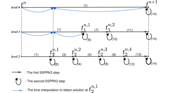
The idea and the order of steps of adaptive SSPRK2 are illustrated on the example in Fig. 3.6. First, we group all cells $T^{n,\mathcal{M}_{n}}_{j}\in\mathcal{T}^{n,\mathcal{M}_{n}}$ at time $t^{n}$ in cell levels $l=0,1,..,L$ based on their sizes. We define cell levels at $t^{n}$ in mesh $\mathcal{T}^{n,\mathcal{M}_{n}}$ as follows. A cell $T^{n,\mathcal{M}_{n}}_{j}\in\mathcal{T}^{n,\mathcal{M}_{n}}$ belongs to the level $l$ , if $l$ is the smallest positive integer satisfying,

2^{l}\geq\dfrac{\displaystyle\max_{j}\left(\displaystyle\min_{k}\left(r_{jk}\right)\right)}{\displaystyle\min_{k}(r_{j,k})},

(3.1)

where $r_{jk},k=1,2,3$ are three altitudes of triangle $T^{n,\mathcal{M}_{n}}_{j}$ . Thus, the cell levels with larger index $l$ will contain finer cells which will require a smaller time step (2.8) for the evolution from $t^{n}\to t^{n+1}$ . Next, at $t^{n}$ , we define the reference time step $\Delta t$ as the local time step on the coarsest level $l=0$ of cells in the mesh $\mathcal{T}^{n,\mathcal{M}_{n}}$ by considering the CFL-type condition (2.8) locally on level $l=0$ . Namely, define first $a_{max}$ ,

a_{max}:=\displaystyle\max_{j,k}(a^{\rm in}_{jk},a^{\rm out}_{jk}),

(3.2)

where $(a^{\rm in}_{jk},a^{\rm out}_{jk})$ are the local one-sided speeds of propagation (2.7) at $t^{n}$ for sides $k=1,2,3$ in the triangle $T^{n,\mathcal{M}_{n}}_{j}\in\mathcal{T}^{n,\mathcal{M}_{n}}$ . Then, the reference time step $\Delta t$ is computed as,

\displaystyle\Delta t\equiv\Delta t^{n,0}_{0}=\frac{0.9\displaystyle\max_{j}\left(\displaystyle\min_{k}\left(r_{jk}\right)\right)}{6a_{max}}.

(3.3)

We set, $t^{n+1}=t^{n}+\Delta t$ .

Assume next, that $\mathcal{P}_{l}$ is the number of steps taken on higher levels $l=1,..L$ to evolve from $t^{n}$ to $t^{n+1},$ namely $[t^{n},t^{n+1}]=\cup[t_{l}^{n,p},t_{l}^{n,p+1}],p=0,...,\mathcal{P}_{l}-1$ with $t^{n,0}_{l}\equiv t^{n}$ , $t_{l}^{n,\mathcal{P}_{l}}\equiv t^{n+1}\quad\forall l$ . We define the local time step for cells on these levels $l=1,...,L$ as,

\Delta t^{n,p}_{l}=\dfrac{2^{-l}\Delta t}{\max(\mu^{n,p}_{l},1)},

(3.4)

where parameter $\mu^{n,p}_{l}$ takes into account change in the local one-sided speeds of the propagation,

\mu^{n,p}_{l}=\dfrac{\displaystyle\max_{j,k}(a^{\rm in}_{jk},a^{\rm out}_{jk})^{n,p}_{l}}{a_{max}},

where $(a^{\rm in}_{jk},a^{\rm out}_{jk})^{n,p}_{l}$ are the local one-sided speeds of propagation at $t^{n,p}_{l}$ of the cell $T^{n,\mathcal{M}_{n}}_{j}$ in the level $l$ . Therefore, on each cell $T^{n,\mathcal{M}_{n}}_{j}$ of level $l$ , for each substep $[t_{l}^{n,p},t_{l}^{n,p+1}]\equiv[t_{l}^{n,p},t_{l}^{n,p}+\Delta t_{l}^{n,p}],p=0,1,2,3,...,\mathcal{P}_{l}-1$ of the evolution from $t^{n}$ to $t^{n+1}$ , we apply the following two adaptive steps of SSPRK2 method,


$\displaystyle\hbox{\vbox{\hrule height=0.5pt\kern 1.72218pt\hbox{\kern-0.50003pt$\bm{U}$\kern-0.50003pt}}}_{j}^{(1)}$	$\displaystyle=\hbox{\vbox{\hrule height=0.5pt\kern 1.72218pt\hbox{\kern-0.50003pt$\bm{U}$\kern-0.50003pt}}}_{j}^{n,p}-\frac{1}{\|T^{n,\mathcal{M}_{n}}_{j}\|}\sum_{k=1}^{3}\Delta t^{n,p}_{jk}{\bm{H}}^{n,p}_{jk}+\Delta t_{l}^{n,p}\,\hbox{\vbox{\hrule height=0.5pt\kern 1.72218pt\hbox{\kern-0.50003pt$\bm{S}$\kern-0.50003pt}}}^{n,p}_{j}:={\bm{R}}(\hbox{\vbox{\hrule height=0.5pt\kern 1.72218pt\hbox{\kern-0.50003pt$\bm{U}$\kern-0.50003pt}}}_{j}^{n,p},\Delta t_{l}^{n,p}),$	(3.5a)
$\displaystyle\hbox{\vbox{\hrule height=0.5pt\kern 1.72218pt\hbox{\kern-0.50003pt$\bm{U}$\kern-0.50003pt}}}_{j}^{n,p+1}$	$\displaystyle=\dfrac{1}{2}\hbox{\vbox{\hrule height=0.5pt\kern 1.72218pt\hbox{\kern-0.50003pt$\bm{U}$\kern-0.50003pt}}}_{j}^{n,p}+\dfrac{1}{2}{\bm{R}}(\hbox{\vbox{\hrule height=0.5pt\kern 1.72218pt\hbox{\kern-0.50003pt$\bm{U}$\kern-0.50003pt}}}_{j}^{(1)},\Delta t_{l}^{n,p}),$	(3.5b)

Here, $\Delta t_{l}^{n,p}$ is the local time step of the cells of level $l$ at time $t_{l}^{n,p}$ (3.4), and $\Delta t^{n,p}_{jk}$ is the “draining” time step in cell $T^{n,\mathcal{M}_{n}}_{j}$ for the local time step $\Delta t_{l}^{n,p}$ in level $l$ . The flux term ${\bm{H}}^{n,p}_{jk}$ in (3.5a) -(3.5b) is the flux (2.3) computed at $t=t^{n,p}_{l}$ . The source term $\hbox{\vbox{\hrule height=0.5pt\kern 1.72218pt\hbox{\kern-0.50003pt${\bm{S}}$\kern-0.50003pt}}}^{n,p}_{j}$ in (3.5a) -(3.5b) is the source (2.10) - (2.11) computed at $t=t^{n,p}_{l}$ with the time step $\Delta t_{l}^{n,p}$ and with the corresponding local “draining” time step $\Delta t^{n,p}_{jk}$ . Note that, $\hbox{\vbox{\hrule height=0.5pt\kern 1.72218pt\hbox{\kern-0.50003pt$\bm{U}$\kern-0.50003pt}}}_{j}^{n,0}\equiv\hbox{\vbox{\hrule height=0.5pt\kern 1.72218pt\hbox{\kern-0.50003pt$\bm{U}$\kern-0.50003pt}}}_{j}^{n}$ and $\hbox{\vbox{\hrule height=0.5pt\kern 1.72218pt\hbox{\kern-0.50003pt$\bm{U}$\kern-0.50003pt}}}_{j}^{n,\mathcal{P}_{l}}\equiv\hbox{\vbox{\hrule height=0.5pt\kern 1.72218pt\hbox{\kern-0.50003pt$\bm{U}$\kern-0.50003pt}}}_{j}^{n+1}$ .

Remark 3.1

If cells from different cell levels are neighbors, we use linear interpolation in time to match the time levels of such cells, see also Fig. 3.6, for the illustration of the interpolation.

3.4 A Posteriori Error Estimator

Here, using the idea of Weak Local Residual (WLR) from [45, 24], we will derive local error estimator that is used as the robust indicator for the adaptive mesh refinement in our work.

Let us recall that the weak form of the mass conservation equation for the system (2.1) in $\Omega\times[0,T]$ takes the integral form,

\int_{0}^{T}\int_{\Omega}(w\phi_{t}(x,y,t)+hu\phi_{x}(x,y,t)+hv\phi_{y}(x,y,t)d\Omega dt+\int_{\Omega}w(x,y,0)\phi(x,y,0)d\Omega=0,

(3.6)

for all sufficiently smooth test functions $\phi(x,y,t)$ with compact support on $\Omega\times[0,T)$ .

Consider example of localized test function in time and space,

\displaystyle\phi^{n+\frac{1}{2}}_{i}(x,y,t)=\frac{1}{\Delta}f_{i}(x,y)f^{n+\frac{1}{2}}(t),

(3.7)

where $\Delta:=\max(\displaystyle\max_{j,k}(r_{jk}),\Delta t)$ , $\Delta t=t^{n+1}-t^{n}=t^{n+\frac{1}{2}}-t^{n-\frac{1}{2}},n=1,2,3...$ , and $r_{jk}$ are the heights of the triangle/cell $T^{n,\mathcal{M}_{n}}_{j}\in\mathcal{T}^{n,\mathcal{M}_{n}}$ . Function $f^{n+\frac{1}{2}}(t)$ is a linear function in time with a local support defined as,

\displaystyle f^{n+\frac{1}{2}}(t)

\displaystyle=\begin{cases}\dfrac{t-t^{n-\frac{1}{2}}}{\Delta t},&\mbox{if}\quad t^{n-\frac{1}{2}}\leq t\leq t^{n+\frac{1}{2}},\\ \\ \dfrac{t^{n+\frac{3}{2}}-t}{\Delta t},&\mbox{if}\quad t^{n+\frac{1}{2}}\leq t\leq t^{n+\frac{3}{2}},\\ \\ 0,&\mbox{otherwise}.\end{cases}

(3.8)

Function $f_{i}(x,y),i=1,2,3,...$ is a “hat function”, namely, a piecewise linear function with compact support over all triangles with common vertex $N_{i}=(\widetilde{x}_{i},\widetilde{y}_{i})$ . The function $f_{i}(x,y)$ takes value $1$ at the vertex $N_{i}$ and $0$ at all other nodes. More precisely, assume that there are $C_{i}$ triangles $T^{n,\mathcal{M}_{n}}_{j_{1}}$ , $T^{n,\mathcal{M}_{n}}_{j_{2}}$ , $T^{n,\mathcal{M}_{n}}_{j_{3}}$ ,…, $T^{n,\mathcal{M}_{n}}_{j_{C_{i}}}\in\mathcal{T}^{n,\mathcal{M}_{n}}$ which share common vertex $N_{i}$ . Thus, the function $f_{i}(x,y)$ is defined as,

\displaystyle f_{i}(x,y)

\displaystyle=\begin{cases}a^{(i)}_{c}(x-\widetilde{x}_{i})+b^{(i)}_{c}(y-\widetilde{y}_{i})+1,&\mbox{if}\quad(x,y)\in T^{n,\mathcal{M}_{n}}_{j_{c}},\quad c=1,2,...C_{i}\\ 0,&\mbox{otherwise}\end{cases},

(3.9)

The quantity $(a^{(i)}_{c},b^{(i)}_{c})$ is the gradient of the linear piece of $f_{i}(x,y)$ restricted to $T^{n,\mathcal{M}_{n}}_{j_{c}}$ ,

	$\displaystyle a^{(i)}_{c}$	$\displaystyle=\dfrac{\widetilde{y}_{2}-\widetilde{y}_{3}}{(\widetilde{y}_{3}-\widetilde{y}_{i})(\widetilde{x}_{2}-\widetilde{x}_{i})-(\widetilde{y}_{2}-\widetilde{y}_{i})(\widetilde{x}_{3}-\widetilde{x}_{i})},$		(3.10)
	$\displaystyle b^{(i)}_{c}$	$\displaystyle=\dfrac{\widetilde{x}_{3}-\widetilde{x}_{2}}{(\widetilde{y}_{3}-\widetilde{y}_{i})(\widetilde{x}_{2}-\widetilde{x}_{i})-(\widetilde{y}_{2}-\widetilde{y}_{i})(\widetilde{x}_{3}-\widetilde{x}_{i})},$		(3.10)

where $N_{i}=(\widetilde{x}_{i},\widetilde{y}_{i}),(\widetilde{x}_{2},\widetilde{y}_{2}),$ and $(\widetilde{x}_{3},\widetilde{y}_{3})$ are the three vertices of triangle $T^{n,\mathcal{M}_{n}}_{j_{c}}$ . Next, define the following piecewise constant approximation for the solution $\bm{U}=(w,hu,hv)$ ,

\bm{U}^{\Delta}:=\hbox{\vbox{\hrule height=0.5pt\kern 1.72218pt\hbox{\kern-0.50003pt$\bm{U}$\kern-0.50003pt}}}_{j_{c}}^{n},\mbox{ if }(x,y,t)\in T^{n,\mathcal{M}_{n}}_{j_{c}}\times[t^{n-\frac{1}{2}},t^{n+\frac{1}{2}}].

(3.11)

Now, using the localized test function $\phi^{n+\frac{1}{2}}_{i}(x,y,t)$ , (3.7) together with the piecewise constant approximation $\bm{U}^{\Delta}$ , (3.11) in (3.6), we can define the weak form of the truncation error, (WLR), which will be used as the error indicator for refinement/de-refinement in the adaptive grid,

	$\displaystyle E^{n+\frac{1}{2}}_{i}:=E(\bm{U}^{\Delta},\phi^{n+\frac{1}{2}}_{i})$	$\displaystyle=\sum_{c=1}^{C_{i}}\int_{t^{n-\frac{1}{2}}}^{t^{n+\frac{1}{2}}}\int_{T^{n,\mathcal{M}_{n}}_{j_{c}}}(\hbox{\vbox{\hrule height=0.5pt\kern 1.72218pt\hbox{\kern-0.50003pt$w$\kern-0.50003pt}}}^{n}_{j_{c}}(\phi^{n+\frac{1}{2}}_{i})_{t}+(\hbox{\vbox{\hrule height=0.5pt\kern 1.72218pt\hbox{\kern-0.50003pt$hu$\kern-0.50003pt}}})^{n}_{j_{c}}(\phi^{n+\frac{1}{2}}_{i})_{x}+(\hbox{\vbox{\hrule height=0.5pt\kern 1.72218pt\hbox{\kern-0.50003pt$hv$\kern-0.50003pt}}})^{n}_{j_{c}}(\phi^{n+\frac{1}{2}}_{i})_{y})d\Omega dt$		(3.12)
		$\displaystyle+\sum_{c=1}^{C_{i}}\int_{t^{n+\frac{1}{2}}}^{t^{n+\frac{3}{2}}}\int_{T^{n,\mathcal{M}_{n}}_{j_{c}}}(\hbox{\vbox{\hrule height=0.5pt\kern 1.72218pt\hbox{\kern-0.50003pt$w$\kern-0.50003pt}}}^{n+1}_{j_{c}}(\phi^{n+\frac{1}{2}}_{i})_{t}+(\hbox{\vbox{\hrule height=0.5pt\kern 1.72218pt\hbox{\kern-0.50003pt$hu$\kern-0.50003pt}}})^{n+1}_{j_{c}}(\phi^{n+\frac{1}{2}}_{i})_{x}+(\hbox{\vbox{\hrule height=0.5pt\kern 1.72218pt\hbox{\kern-0.50003pt$hv$\kern-0.50003pt}}})^{n+1}_{j_{c}}(\phi^{n+\frac{1}{2}}_{i})_{y})d\Omega dt.$		(3.12)

After straightforward calculations, the WLR error $E^{n+\frac{1}{2}}_{i}$ on mesh $\mathcal{T}^{n,\mathcal{M}_{n}}$ is given by the formula,

$\displaystyle E^{n+\frac{1}{2}}_{i}$	$\displaystyle=\frac{1}{\Delta}(\mathcal{U}^{n+\frac{1}{2}}_{i}+\mathcal{F}^{n+\frac{1}{2}}_{i}+\mathcal{G}^{n+\frac{1}{2}}_{i}),$	(3.13)
$\displaystyle\mathcal{\bm{U}}^{n+\frac{1}{2}}_{i}$	$\displaystyle=\sum\limits_{c=1}^{C_{i}}\frac{1}{3}\|T^{n,\mathcal{M}_{n}}_{j_{c}}\|(\hbox{\vbox{\hrule height=0.5pt\kern 1.72218pt\hbox{\kern-0.50003pt$w$\kern-0.50003pt}}}^{n}_{j_{c}}-\hbox{\vbox{\hrule height=0.5pt\kern 1.72218pt\hbox{\kern-0.50003pt$w$\kern-0.50003pt}}}^{n+1}_{j_{c}}),$
$\displaystyle\mathcal{F}^{n+\frac{1}{2}}_{i}$	$\displaystyle=\sum\limits_{c=1}^{C_{i}}a^{(i)}_{c}\frac{\Delta t}{2}\|T^{n,\mathcal{M}_{n}}_{j_{c}}\|((\hbox{\vbox{\hrule height=0.5pt\kern 1.72218pt\hbox{\kern-0.50003pt$hu$\kern-0.50003pt}}})^{n}_{j_{c}}+(\hbox{\vbox{\hrule height=0.5pt\kern 1.72218pt\hbox{\kern-0.50003pt$hu$\kern-0.50003pt}}})^{n+1}_{j_{c}}),$
$\displaystyle\mathcal{G}^{n+\frac{1}{2}}_{i}$	$\displaystyle=\sum\limits_{c=1}^{C_{i}}b^{(i)}_{c}\frac{\Delta t}{2}\|T^{n,\mathcal{M}_{n}}_{j_{c}}\|((\hbox{\vbox{\hrule height=0.5pt\kern 1.72218pt\hbox{\kern-0.50003pt$hv$\kern-0.50003pt}}})^{n}_{j_{c}}+(\hbox{\vbox{\hrule height=0.5pt\kern 1.72218pt\hbox{\kern-0.50003pt$hv$\kern-0.50003pt}}})^{n+1}_{j_{c}}).$

The error in a cell $T^{n,\mathcal{M}_{n}}_{j}\in\mathcal{T}^{n.\mathcal{M}_{n}}$ is given by,

e_{j}=\max_{k}\left|E^{n+\frac{1}{2}}_{jk}\right|,\quad k=1,2,3,

(3.14)

where $E^{n+\frac{1}{2}}_{jk}$ is the WLR error computed in (3.13) at a node $k$ of triangle $T_{j}$ .

In our numerical experiments, we define an error tolerance, $\omega$ as,

\omega=\sigma\max_{j}(e_{j}),

(3.15)

where $\sigma<1$ is a given problem-dependent constant (see Section 4), and $e_{j}$ is the WLR error in the triangle $T^{n.\mathcal{M}_{n}}_{j}$ , (3.14). The error $e_{j}$ in each cell $T^{n.\mathcal{M}_{n}}_{j}\in\mathcal{T}^{n,\mathcal{M}_{n}}$ is compared to the error tolerance (3.15), and the cell is either “flagged” for refinement/de-refinement or “no-change”.

Note that, in this work, we consider only the equation (1.1a) to obtain WLR error. The full system of shallow water equations can be used to derive WLR too, however it will make the computation of the error indicator more complex and more expensive.

4 Numerical Examples

In this section, we illustrate the performance of the designed adaptive central-upwind scheme. We compare the results of the adaptive central-upwind scheme developed in this work with the results of the central-upwind scheme from [36] on uniform triangular meshes (example of such uniform triangular mesh is outlined in Fig. 4.1). In addition, in all experiments, we compute ratio, $\mathcal{R}_{CPU}=\frac{CPU_{uniform}}{CPU_{adaptive}}$ , which is the ratio of the CPU times of the central-upwind algorithm without adaptivity to the CPU time of the adaptive central-upwind algorithm. To compare $L^{1}$ -errors, as well as to compare the CPU times and to compute $\mathcal{R}_{CPU}$ , we consider uniform mesh and the adaptive mesh with the same size of the smallest cells. More precisely, in Table 4.1, $L^{1}$ -errors, and in Tables 4.2-4.7, $\mathcal{R}_{CPU}$ are computed using the uniform meshes $2\times N\times N,N=100,200,400$ and using the corresponding adaptive meshes which are obtained from the coarser uniform mesh $2\times N/2^{\mathcal{M}}\times N/2^{\mathcal{M}}$ ( $\mathcal{M}=1,2$ is the highest level of refinement in the adaptive mesh). In Example 4.1 and the first two cases in Example 4.2 with (4.1)-(4.2), the gravitational acceleration is set, $g=1.0$ , while in the last case of Example 4.2 with (4.3)-(4.4) and Example 4.3, we take $g=9.8$ . We set the desingularization parameters $\tau$ and $\varepsilon$ for calculations of the velocity components $u$ and $v$ to be $\tau=\max_{j}\{|T^{n,\mathcal{M}_{n}}_{j}|^{2}\}$ and $\varepsilon=10^{-4}$ , except for the Example 4.2, (4.3)-(4.4), where $\varepsilon=10^{-2}$ (see Section 2.1 formula (2.6) in [36]).

4.1 Example 1—Accuracy Test

Here, we consider the example from [6], and we verify experimentally the order of accuracy of the designed adaptive central-upwind scheme. We also compare the computational efficiency of the adaptive central-upwind scheme and the central-upwind scheme without adaptivity on uniform and non-uniform triangular meshes.

We consider the following initial data and the bottom topography,

w(x,y,0)=1,\quad u(x,y,0)=0.3,\quad v(x,y,0)=0,

B(x,y)=0.5\exp(-25(x-1)^{2}-50(y-0.5)^{2}).

The computational domain is $[0,2]\times[0,1]$ . A zero-order extrapolation is used at all boundaries. The error tolerance (3.15) for the mesh refinement in this example is set to $\omega=0.01\max_{j}(e_{j})$ .

From the result reported in [6], by $t=0.07$ , the numerical solution reaches the steady state. In Fig. 4.2 (left column), we show the numerical solution of water surface at $t=0.07$ . The solution is computed using the central-upwind scheme on uniform meshes on Fig. 4.2 (a, b) and using the adaptive central-upwind scheme on Fig. 4.2 (c, d). The adaptive meshes in Fig. 4.2 are obtained from the uniform mesh $2\times 25\times 25$ , Fig. 4.2 (a). The adaptive mesh with one level of refinement $\mathcal{M}=1$ (as the highest level of refinement) is on Fig. 4.2 (c), and with two levels of refinement $\mathcal{M}=2$ (as the highest level of refinement) is on Fig. 4.2 (d).

Next, in Table 4.1 we compute the $L^{1}$ -errors of the central-upwind scheme on uniform meshes and of the adaptive central-upwind scheme. To obtain the errors, the reference solution is calculated on the uniform mesh with $2\times 800\times 800$ triangles. In Table 4.2, we present the $\mathcal{R}_{CPU}$ ratio to compare the computational efficiency of the two methods. From Table 4.1 and Table 4.2, we observe that the adaptive algorithm produces similar accuracy as the scheme on fixed uniform triangular meshes, but at a less computational cost. Also, as expected, the adaptive central-upwind scheme achieves second-order accuracy in space, similar to the central-upwind scheme without adaptivity.

algorithm without adaptivity			adaptive algorithm
			one level $\mathcal{M}=1$			two levels $\mathcal{M}=2$
cells	$L^{1}$ -error	rate	cells	$L^{1}$ -error	rate	cells	$L^{1}$ -error	rate
$2\times 100\times 100$	2.22e-05		11,808	2.33e-05		10,404	3.41e-05
$2\times 200\times 200$	4.74e-06	2.22	46,892	5.62e-06	2.05	40,728	5.91e-06	2.53
$2\times 400\times 400$	9.84e-07	2.26	187,726	1.55e-06	1.85	160,846	1.54e-06	1.94

Table 4.1: Example 1:

L^{1}

-errors of the water surface

w

t=0.07

, and the convergence rates of the central-upwind scheme without adaptivity (uniform mesh

2\times N\times N,N=100,200,400

) and the adaptive scheme (the corresponding adaptive mesh is reconstructed from the uniform mesh

2\times N/2^{\mathcal{M}}\times N/2^{\mathcal{M}}

uniform mesh	adaptive mesh $\mathcal{M}=1$	$\mathcal{R}_{CPU}$ with $\mathcal{M}=1$		adaptive mesh $\mathcal{M}=2$	$\mathcal{R}_{CPU}$ with $\mathcal{M}=2$
(cells)	(cells)	total	without grid generation	(cells)	total	without grid generation
$2\times 100\times 100$	11,808	2.18	2.36	10,404	2.58	2.70
$2\times 200\times 200$	46,892	1.85	2.05	40,728	2.48	2.62
$2\times 400\times 400$	187,726	1.77	1.98	160,846	2.25	2.40
$\mathcal{R}_{CPU}$ average:		1.93	2.13		2.44	2.57

Table 4.2: Example 1:

\mathcal{R}_{CPU}

ratio at

t=0.07

, where for adaptive central-upwind scheme, we consider the total CPU times and CPU times without the grid generation.

In addition, we will use this example to show that the adaptive central-upwind scheme is also effective on the unstructured triangular meshes. On Fig. 4.3 (left), we plot the numerical solution at $t=0.07$ computed using the central-upwind method on a non-uniform mesh, Fig. 4.3 (a), the adaptive scheme with one level of refinement, Fig. 4.3 (b) and the adaptive scheme with two levels of refinement, Fig. 4.3 (c). The adaptive meshes on Fig. 4.3 (b, c) are reconstructed from the non-uniform mesh shown on the right Fig. 4.3 (a).

We then recompute the accuracy of the solution, see Table 4.3, and the CPU time ratio, see Table 4.4, obtained by using the non-uniform meshes. From Table 4.3 and Table 4.4, we observe that the advantage of the adaptive scheme is still maintained on non-uniform meshes as it reduces the computational cost of the method. Next, we compare the results presented in Table 4.3 and in Table 4.1. As expected, we see that the errors obtained by using scheme on non-uniform meshes is slightly larger than the ones using the corresponding uniform meshes (with approximately the same number of cells).

algorithm without adaptivity			adaptive algorithm
			one level $\mathcal{M}=1$			two levels $\mathcal{M}=2$
cells	$L^{1}$ -error	rate	cells	$L^{1}$ -error	rate	cells	$L^{1}$ -error	rate
22,438	2.64e-05		13,036	2.53e-05		11,630	3.59e-05
90,434	6.53e-06	2.02	51,656	5.98e-06	2.08	44,400	7.06e-06	2.35
314,708	1.15e-06	2.51	204,044	1.68e-06	1.83	176,278	1.60e-06	2.14

Table 4.3: Example 1:

L^{1}

-errors of the water surface

w

t=0.07

, and the convergence rates of the central-upwind scheme without adaptivity in non-uniform mesh and the adaptive scheme (the corresponding adaptive meshes has the same size of the smallest cells with the compared non-uniform meshes).

Non-uniform and non-adaptive mesh	adaptive mesh $\mathcal{M}=1$	$\mathcal{R}_{CPU}$ with $\mathcal{M}=1$		adaptive mesh $\mathcal{M}=2$	$\mathcal{R}_{CPU}$ with $\mathcal{M}=2$
(cells)	(cells)	total	without grid generation	(cells)	total	without grid generation
22,438	13,036	1.86	1.94	11,630	3.77	3.90
90,434	51,656	2.20	2.20	44,400	3.34	3.43
314,708	204,044	2.45	2.57	176,278	3.36	3.46
$\mathcal{R}_{CPU}$ average:		2.17	2.24		3.49	3.60

Table 4.4: Example 1:

\mathcal{R}_{CPU}

ratio at

t=0.07

, where for adaptive central-upwind scheme, we consider the total CPU times and CPU times without the grid generation in non-uniform meshes.

4.2 Example 2—Well-Balanced Tests and Test with Wet/Dry Interfaces

The first numerical example here was proposed in [33] to test capability of the numerical scheme to accurately resolve small perturbations of a steady state solution. We take a computational domain $[0,2]\times[0,1]$ and the bottom topography,

B(x,y)=0.8\exp(-5(x-0.9)^{2}-50(y-0.5)^{2}).

(4.1)

The initial conditions describe a flat surface of water with a small perturbation in $0.05<x<0.15$ :

w(x,y,0)=\begin{cases}1+\epsilon,\quad&0.05<x<0.15,\\ 1,&\mbox{otherwise,}\end{cases}\quad u(x,y,0)\equiv v(x,y,0)\equiv 0,

(4.2)

where $\epsilon$ is the perturbation height. We have used the zero-order extrapolation at the right and the left boundaries of the domain and the periodic boundary conditions for the top and the bottom ones.

To verify well-balanced property of the adaptive scheme, we first consider a very small perturbation $\epsilon=10^{-14}$ . The adaptive meshes with levels $\mathcal{M}=1,2$ are obtained from a coarse uniform mesh $2\times 25\times 25$ . The threshold for mesh refinement in this example is $\displaystyle\omega=0.1\max_{j}(e_{j})$ . We plot $\displaystyle\max_{x,y}(w-1)$ as a function of time for the central-upwind scheme without adaptivity on uniform mesh in Fig. 4.4 (a), for the adaptive central-upwind scheme with $\mathcal{M}=1$ in Fig. 4.4 (b), and with $\mathcal{M}=2$ in Fig. 4.4 (c). The results of the test show that the adaptive scheme is stable and preserves numerically the balance between the fluxes and the source term, similar to the scheme without adaptivity.

In the next numerical test, we take a larger perturbation value $\epsilon=10^{-2}$ . The purpose of this test is to demonstrate the capability of the adaptive algorithm to resolve the small scale features of the solution. In Fig. 4.5, we plot the water surface $w$ obtained by the method without adaptivity on two uniform meshes $2\times 100\times 100$ (left) and $2\times 200\times 200$ (right) at $t=0.6,0.9,1.2,1.5$ and $1.8$ . The computed solutions of the water surface exhibit a right-going disturbance propagating past the hump. We then apply the adaptive algorithm and plot the numerical solution of the water surface $w$ on selected meshes at different times in Fig. 4.6 (left) with $\mathcal{M}=1$ and in Fig. 4.7 (left) with $\mathcal{M}=2$ (the starting grid was a uniform mesh with $2\times 100\times 100$ and the threshold is $\displaystyle\omega=0.1\max_{j}(e_{j})$ ). We observe from Fig. 4.5, Fig. 4.6 and Fig. 4.7 that the adaptive central-upwind scheme delivers high resolution of the complex features of a small perturbation of the ”lake-at-rest” steady state. We note also, that by increasing the level of refinement from $\mathcal{M}=1$ to $\mathcal{M}=2$ , the number of cells in the mesh increases from $30,912$ cells with $\mathcal{M}=1$ to $66,097$ cells with $\mathcal{M}=2$ , but the accuracy is clearly improved with higher resolution as seen in Fig. 4.6 and Fig. 4.7. We also present the corresponding adaptive meshes in Fig. 4.6 (right) and in Fig. 4.7 (right). Clearly, the meshes are adapted to the behavior of the flow during time evolution from $t=0.6$ to $t=1.8$ . This confirms the ability of the WLR error estimator to detect location of the steep local gradients in the solution.

To demonstrate further the advantage of the adaptive scheme, we have compared the CPU times of the central-upwind scheme without adaptivity and with adaptivity for the solution at $t=0.9$ . The computed $\mathcal{R}_{CPU}$ ratios are presented in Table 4.5. The computed ratios $\mathcal{R}_{CPU}$ show that the adaptive central-upwind scheme can reduce the numerical cost by about three times with $\mathcal{M}=1$ and by about five times with $\mathcal{M}=2$ in comparison with the cost of the algorithm without adaptivity.

uniform mesh (cells)	adaptive mesh $\mathcal{M}=1$ (cells)	$\mathcal{R}_{CPU}$ with $\mathcal{M}=1$	adaptive mesh $\mathcal{M}=2$ (cells)	$\mathcal{R}_{CPU}$ with $\mathcal{M}=2$
$2\times 100\times 100$	9,127	3.50	8,274	4.06
$2\times 200\times 200$	30,912	2.06	21,131	5.29
$2\times 400\times 400$	108,297	3.67	66,097	6.38
$\mathcal{R}_{CPU}$ average:		3.07		5.24

Table 4.5: Example 2: The

R_{CPU}

ratio obtained in solving the IVP (1.1a)-(1.1c),(4.1)-(4.2) with

\epsilon=10^{-2}

t=0.9

In the final test, we consider an example with a small perturbation that propagates around an island. Similar examples were considered in [6, 36]. We consider a hump partially submerged in water so that there is a disk-shaped island at the origin, see Fig. 4.8. Hence, the bottom topography is given by

B(x,y)=\begin{cases}1.1,\quad&r\leq 0.1,\\ 11\times(0.2-r)\quad&0.1<r\leq 0.2,\\ 0,&\mbox{otherwise,}\end{cases}\quad r:=\sqrt{(x-0.5)^{2}+(y-0.5)^{2}}.

(4.3)

We consider the following initial condition,

w(x,y,0)=\begin{cases}1+\epsilon,\quad&0.1<x<0.2,\\ \max(1,B(x,y)),&\mbox{otherwise,}\end{cases}\quad u(x,y,0)\equiv v(x,y,0)\equiv 0,

(4.4)

where $\epsilon=10^{-2}$ is the perturbation height. The homogeneous Neumann boundary conditions are used at all boundaries.

We first obtain the water surface using central-upwind scheme without adaptivity. Different to the results in the submerged plateau case (4.1)-(4.2), the right-going disturbance bends around the island and is being reflected by the island.

We then compare with the performance of the adaptive scheme in this case. The adaptive grids are generated from the uniform mesh $2\times 100\times 100$ using the threshold $\omega=0.001\max_{j}(e_{j})$ for one level of refinement $\mathcal{M}=1$ and $\omega=0.01\max_{j}(e_{j})$ for $\mathcal{M}=2$ . In Fig. 4.10 (left) and Fig. 4.11 (left), we plot the results for $w$ (left) obtained by the adaptive scheme and the corresponding adaptive meshes (right). The results are similar to the results of the central-upwind scheme without adaptivity in Fig. 4.9. There are no non-physical spurious waves generated at the wet/dry front. The well-balanced property, positivity and stability of the proposed adaptive central-upwind method are maintained with the adaptive mesh refinement. As in previous examples, WLR error estimator accurately detects regions in the domain which are marked for adaptive refinement/coarsening.

Next, in Table 4.6, we present ratio of CPU times $\mathcal{R}_{CPU}$ to compute the solution at $t=0.1$ by the central-upwind method without adaptivity and by the adaptive algorithm. In order to compare the computational costs and calculate $\mathcal{R}_{CPU}$ , we consider uniform and adaptive meshes with the same size of the smallest cells. From Table 4.6, one can see that the adaptive algorithm reduces the CPU times up to four times. In our experiments, we considered only $\mathcal{M}=1$ and $\mathcal{M}=2$ , but one can consider higher levels of refinement to further enhance the accuracy of the numerical solution at the reduced computational cost.

uniform mesh (cells)	adaptive mesh $\mathcal{M}=1$ (cells)	$\mathcal{R}_{CPU}$ with $\mathcal{M}=1$	adaptive mesh $\mathcal{M}=2$ (cells)	$\mathcal{R}_{CPU}$ with $\mathcal{M}=2$
$2\times 100\times 100$	11,831	1.91	6,155	3.04
$2\times 200\times 200$	31,050	2.08	25,753	3.14
$2\times 400\times 400$	154,616	3.16	94,357	5.82
$\mathcal{R}_{CPU}$ average:		2.38		4.00

Table 4.6: Example 2: The

R_{CPU}

ratio for solving the IVP (1.1a)-(1.1c), (4.3)-(4.4) at

t=0.1

Finally, we illustrate the advantages of WLR error as the error indicator, and hence compare it with another example of the error indicator which uses the unlimited gradients of the water surface $(w_{x},w_{y})$ , see e.g. [19]. We continue to consider the IVP (1.1a)-(1.1c),(4.1)-(4.2). In Fig. 4.12 (left column), we first present the contour plots of water surface $w$ computed at $t=0.14$ and $t=0.2$ using the meshes obtained by WLR error indicator, Fig. 4.12 (middle column). The adaptive meshes in Fig. 4.12 (middle and right columns) are reconstructed from the uniform mesh $2\times 100\times 100$ , respectively, by using the WLR error indicator and the gradient indicator. For WLR error, we apply the threshold $\omega=0.01\max_{j}(e_{j})$ and refine a cell $T_{j}$ if local WLR error $e_{j}>\omega\times 2^{m-1}$ for $m\leq\mathcal{M}=3$ levels. For the gradient indicator, a cell $T_{j}$ is flagged for $m,m\leq 3,$ levels of refinement if it has $(w_{x})_{j}^{2}+(w_{y})_{j}^{2}>0.0005\times 2^{m-1}$ . From Fig. 4.12, we can observe that the WLR error indicator captures more subtle features of the solution than the error indicator based on the gradient.

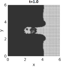
4.3 Example 3—Dam Break Test

In example 3 taken from [36], we simulate the propagation of the dam-break flood wave which produces a moving wet/dry fronts over an irregular dry bed with three obstacles. The test allows to verify capability of the proposed adaptive algorithm to handle wet/dry interfaces. The bottom topography is defined by,

B(x,y)=\max\left[0.5e^{-8(x-2)^{2}-10(y-3)^{2}},0.2e^{-3(x-4)^{2}-4(y-4.8)^{2}},0.2e^{-3(x-4)^{2}-4(y-1.2)^{2}}\right],

(4.5)

in the computational domain is $[0,6]\times[0,6]$ . At $t=0$ , an upstream reservoir in the region $[0,1]\times[0,6]$ filled with water up to $w(x,y,0)=0.5$ is suddenly released. Hence, the following initial condition is imposed,

w(x,y,0)=\begin{cases}0.5,\quad&0\leq x<1,\\ B(x,y),&\mbox{otherwise,}\end{cases}\quad u(x,y,0)\equiv v(x,y,0)\equiv 0.

(4.6)

In this example, we consider the friction effects by modifying the governing equation (1.1b) and (1.1c) with the Manning friction terms as follows,

\begin{split}(hu)_{t}+\left(hu^{2}+\dfrac{g}{2}h^{2}\right)_{x}+(huv)_{y}=-ghB_{x}-\dfrac{gn^{2}_{b}u\sqrt{u^{2}+v^{2}}}{h^{1/3}},\\ (hv)_{t}+(huv)_{x}+\left(hv^{2}+\dfrac{g}{2}h^{2}\right)_{y}=-ghB_{y}-\dfrac{gn^{2}_{b}v\sqrt{u^{2}+v^{2}}}{h^{1/3}},\end{split}

(4.7)

where $n_{b}=0.01$ is the Manning roughness coefficient. We have used the homogeneous Neumann boundary condition for the left boundary $x=6$ and the solid wall boundary condition for the other boundaries.

We first present the numerical solution computed by applying the central-upwind scheme without the adaptivity [36] on the uniform meshes. Fig. 4.13 and Fig. 4.14 are the 3-D view of the dam-break wave propagation over the initially dry bed obtained respectively on $2\times 100\times 100$ and $2\times 200\times 200$ uniform meshes at different times $t=0.4,0.6,1.0,1.4,2.0,$ and $4.0$ . As can be observed from the figures, the water wave spreads from the reservoir and passes the obstacles. In addition, we plot the contour lines of the water depth for the solutions obtained on the uniform meshes $2\times 100\times 100$ (Fig. 4.15) and $2\times 200\times 200$ (Fig. 4.16). The contour lines clearly show the reflections and interactions of waves.

Now, we continue the test for the proposed adaptive central-upwind method with the refined meshes generated from the uniform mesh $2\times 100\times 100$ . The threshold for the grid refinement is set to $\omega=0.01\max_{j}(e_{j})$ in this example. In Fig. 4.17 and Fig. 4.18, we show the 3-D view of the simulated water computed by the adaptive scheme on the adaptive meshes with two cases of the highest refinement level $\mathcal{M}=1$ and $\mathcal{M}=2$ . The behavior of the wave is similar to the result obtained by the central-upwind scheme without adaptivity, see Fig. 4.13 and Fig. 4.14. This means that the adaptive scheme performs well in simulating the wetting/drying processes. There are no non-physical spurious waves appear as a result of the simulation. We also present the contour lines of the water depth obtained on the adaptive meshes with $\mathcal{M}=1$ (Fig. 4.19) and $\mathcal{M}=2$ (Fig. 4.20). Clearly, the simulated solution captures correctly the reflections and interactions of the waves with no oscillations or disturbances showing up at the wet/dry interfaces. The considered adaptive meshes with $\mathcal{M}=1$ are plotted in Fig. 4.21 and with $\mathcal{M}=2$ in Fig. 4.22. As we expected, the moving refined/de-refined regions match with the wetting and drying processes in the propagation of the flow.

Finally, we present the $R_{CPU}$ ratios at time $t=1.0$ in Table 4.7. The result in Table 4.7 shows that the average cost for the adaptive central-upwind method is about half of the cost for the central-upwind method without adaptivity. Note that at $t=1.0$ , the refined region is larger than half of the computational domain, see Fig. 4.21 and Fig. 4.22. Therefore, the numerical cost is not as remarkably reduced with the adaptive grid as the cost in example 2, see Table 4.6. As illustrated, the adaptive central-upwind method preserves the advantages of the well-balanced positivity preserving central-upwind scheme proposed in [36], but at a less computational cost.

uniform mesh (cells)	adaptive mesh $\mathcal{M}=1$ (cells)	$\mathcal{R}_{CPU}$ with $\mathcal{M}=1$	adaptive mesh $\mathcal{M}=2$ (cells)	$\mathcal{R}_{CPU}$ with $\mathcal{M}=2$
$2\times 100\times 100$	15,064	2.47	14,299	2.64
$2\times 200\times 200$	59,252	1.62	54,518	2.13
$2\times 400\times 400$	238,485	1.53	217,075	1.69
$\mathcal{R}_{CPU}$ average:		1.87		2.02

Table 4.7: Example 3: The

R_{CPU}

ratios at

t=1.0

5 Conclusion

We have developed a new adaptive well-balanced and positivity preserving central-upwind scheme on unstructured traingular meshes for shallow water equations. The designed scheme is an extension and improvement of the scheme in [36]. In addition, as a part of the adaptive algorithm, we obained a robust local error indicator for the efficient mesh refinement strategy. We conducted several challenging numerical tests for shallow water equations and we demonstrated that the new adaptive central-upwind scheme maintains important stability properties (i.e., well-balanced and positivity-preserving properties) and delivers high-accuracy at a reduced computational cost.

References

[1] E. Audusse, F. Bouchut, M.-O. Bristeau, R. Klein, and B. Perthame, A fast and stable well-balanced scheme with hydrostatic reconstruction for shallow water flows, SIAM J. Sci. Comput., 25 (2004), pp. 2050–2065 (electronic).
[2] P. Azerad, J.-L. Guermond, and B. Popov, Well-balanced second-order approximation of the shallow water equation with continuous finite elements, SIAM J. Numer. Anal., 55 (2017), pp. 3203–3224.
[3] A. Bollermann, G. Chen, A. Kurganov, and S. Noelle, A well-balanced reconstruction of wet/dry fronts for the shallow water equations, J. Sci. Comput., 56 (2013), pp. 267–290.
[4] A. Bollermann, S. Noelle, and M. Lukáčová-Medviďová, Finite volume evolution Galerkin methods for the shallow water equations with dry beds, Commun. Comput. Phys., 10 (2011), pp. 371–404.
[5] S. Bryson, Y. Epshteyn, A. Kurganov, and G. Petrova, Central Upwind Scheme on Triangular Grids for the Saint Venant System of Shallow Water Equations, AIP Conference Proceedings, 1389 (2011), pp. 686–689.
[6] S. Bryson, Y. Epshteyn, A. Kurganov, and G. Petrova, Well-balanced positivity preserving central-upwind scheme on triangular grids for the Saint-Venant system, ESAIM Math. Model. Numer. Anal., 45 (2011), pp. 423–446.
[7] S. Bryson and D. Levy, Balanced central schemes for the shallow water equations on unstructured grids, SIAM J. Sci. Comput., 27 (2005), pp. 532–552 (electronic).
[8] S. Bunya, E. J. Kubatko, J. J. Westerink, and C. Dawson, A wetting and drying treatment for the Runge-Kutta discontinuous Galerkin solution to the shallow water equations, Comput. Methods Appl. Mech. Engrg., 198 (2009), pp. 1548–1562.
[9] A. Chertock, Y. Epshteyn, H. Hu, and A. Kurganov, High-order positivity-preserving hybrid finite-volume-finite-difference methods for chemotaxis systems, Adv. Comput. Math., 44 (2018), pp. 327–350.
[10] A. Chertock, K. Fellner, A. Kurganov, A. Lorz, and P. A. Markowich, Sinking, merging and stationary plumes in a coupled chemotaxis-fluid model: a high-resolution numerical approach, Journal of Fluid Mechanics, 694 (2012), pp. 155–190.
[11] A. Chertock, A. Kurganov, and Y. Liu, Central-upwind schemes for the system of shallow water equations with horizontal temperature gradients, Numer. Math., 127 (2014), pp. 595–639.
[12] A. J. C. de Saint-Venant, Thèorie du mouvement non-permanent des eaux, avec application aux crues des rivière at à l’introduction des marèes dans leur lit., C.R. Acad. Sci. Paris, 73 (1871), pp. 147–154.
[13] M. O. Domingues, S. M. Gomes, O. Roussel, and K. Schneider, An adaptive multiresolution scheme with local time stepping for evolutionary pdes, Journal of Computational Physics, 227 (2008), pp. 3758–3780.
[14] R. Donat, M. Martí, A. Martínez-Gavara, and P. Mulet, Well-balanced adaptive mesh refinement for shallow water flows, Journal of Computational Physics, 257 (2014), pp. 937–953.
[15] U. S. Fjordholm, S. Mishra, and E. Tadmor, Energy preserving and energy stable schemes for the shallow water equations, in Foundations of computational mathematics, Hong Kong 2008, vol. 363 of London Math. Soc. Lecture Note Ser., Cambridge Univ. Press, Cambridge, 2009, pp. 93–139.
[16] , Well-balanced and energy stable schemes for the shallow water equations with discontinuous topography, J. Comput. Phys., 230 (2011), pp. 5587–5609.
[17] T. Gallouët, J.-M. Hérard, and N. Seguin, Some approximate Godunov schemes to compute shallow-water equations with topography, Comput. & Fluids, 32 (2003), pp. 479–513.
[18] D. L. George, Finite volume methods and adaptive refinement for tsunami propagation and inundation, Ph.D, University of Washington, (2006).
[19] M. A. Ghazizadeh, A. Mohammadian, and A. Kurganov, An adaptive well-balanced positivity preserving central-upwind scheme on quadtree grids for shallow water equations, Computers $\&$ Fluids, 208 (2020), p. 104633.
[20] S. Gottlieb, C.-W. Shu, and E. Tadmor, Strong stability-preserving high-order time discretization methods, SIAM Rev., 43 (2001), pp. 89–112.
[21] N. Hannoun and V. Alexiades, Issues in adaptive mesh refinement implementation, Electronic Journal of Differential Equations, 15 (2007), pp. 141–151.
[22] S. Jin, A steady-state capturing method for hyperbolic systems with geometrical source terms, M2AN Math. Model. Numer. Anal., 35 (2001), pp. 631–645.
[23] S. Jin and X. Wen, Two interface-type numerical methods for computing hyperbolic systems with geometrical source terms having concentrations, SIAM J. Sci. Comput., 26 (2005), pp. 2079–2101.
[24] S. Karni and A. Kurganov, Local error analysis for approximate solutions of hyperbolic conservation laws, Adv. Comput. Math., 22 (2005), pp. 79–99.
[25] A. Kurganov and D. Levy, Central-upwind schemes for the Saint-Venant system, M2AN Math. Model. Numer. Anal., 36 (2002), pp. 397–425.
[26] A. Kurganov and Y. Liu, New adaptive artificial viscosity method for hyperbolic systems of conservation laws, J. Comput. Phys., 231 (2012), pp. 8114–8132.
[27] A. Kurganov and J. Miller, Central-upwind scheme for Savage-Hutter type model of submarine landslides and generated tsunami waves, Comput. Methods Appl. Math., 14 (2014), pp. 177–201.
[28] A. Kurganov, S. Noelle, and G. Petrova, Semi-discrete central-upwind schemes for hyperbolic conservation laws and Hamilton-Jacobi equations, SIAM J. Sci. Comput., 23 (2001), pp. 707–740.
[29] A. Kurganov and G. Petrova, Central-upwind schemes on triangular grids for hyperbolic systems of conservation laws, Numer. Methods Partial Differential Equations, 21 (2005), pp. 536–552.
[30] A. Kurganov and G. Petrova, A second-order well-balanced positivity preserving scheme for the Saint-Venant system, Commun. Math. Sci., 5 (2007), pp. 133–160.
[31] A. Kurganov and E. Tadmor, New high-resolution central schemes for nonlinear conservation laws and convection-diffusion equations, J. Comput. Phys., 160 (2000), pp. 241–282.
[32] , New high-resolution semi-discrete central schemes for Hamilton-Jacobi equations, J. Comput. Phys., 160 (2000), pp. 720–742.
[33] R. LeVeque, Balancing source terms and flux gradients in high-resolution Godunov methods: the quasi-steady wave-propagation algorithm, J. Comput. Phys., 146 (1998), pp. 346–365.
[34] , Finite volume methods for hyperbolic problems, Cambridge Texts in Applied Mathematics, Cambridge University Press, Cambridge, 2002.
[35] M. Li, P. Guyenne, F. Li, and L. Xu, A positivity-preserving well-balanced central discontinuous Galerkin method for the nonlinear shallow water equations, J. Sci. Comput., 71 (2017), pp. 994–1034.
[36] X. Liu, J. Albright, Y. Epshteyn, and A. Kurganov, Well-balanced positivity preserving central-upwind scheme with a novel wet/dry reconstruction on triangular grids for the Saint-Venant system, Journal of Computational Physics, 374 (2018), pp. 213 – 236.
[37] M. Moreira Lopes, M. O. Domingues, K. Schneider, and O. Mendes, Local time-stepping for adaptive multiresolution using natural extension of runge–kutta methods, Journal of Computational Physics, 382 (2019), pp. 291 – 318.
[38] H. Nessyahu and E. Tadmor, Nonoscillatory central differencing for hyperbolic conservation laws, J. Comput. Phys., 87 (1990), pp. 408–463.
[39] S. Noelle, N. Pankratz, G. Puppo, and J. Natvig, Well-balanced finite volume schemes of arbitrary order of accuracy for shallow water flows, J. Comput. Phys., 213 (2006), pp. 474–499.
[40] B. Perthame and C. Simeoni, A kinetic scheme for the Saint-Venant system with a source term, Calcolo, 38 (2001), pp. 201–231.
[41] G. Russo, Central schemes for balance laws, in Hyperbolic problems: theory, numerics, applications, Vol. I, II (Magdeburg, 2000), vol. 141 of Internat. Ser. Numer. Math., 140, Birkhäuser, Basel, 2001, pp. 821–829.
[42] G. Russo, Central schemes for conservation laws with application to shallow water equations, in Trends and applications of mathematics to mechanics: STAMM 2002, S. Rionero and G. Romano (eds.), (2005), pp. 225–246.
[43] M. L. Sæ tra, A. R. Brodtkorb, and K.-A. Lie, Efficient GPU-implementation of adaptive mesh refinement for the shallow-water equations, J. Sci. Comput., 63 (2015), pp. 23–48.
[44] H. Shirkhani, A. Mohammadian, O. Seidou, and A. Kurganov, A well-balanced positivity-preserving central-upwind scheme for shallow water equations on unstructured quadrilateral grids, Comput. & Fluids, 126 (2016), pp. 25–40.
[45] E. Tadmor, Local error estimates for discontinuous solutions of nonlinear hyperbolic equations, SIAM J. Numer. Anal., 28 (1991), pp. 891–906.
[46] Y. Xing and C.-W. Shu, High order finite difference WENO schemes with the exact conservation property for the shallow water equations, J. Comput. Phys., 208 (2005), pp. 206–227.
[47] , High order well-balanced finite volume WENO schemes and discontinuous Galerkin methods for a class of hyperbolic systems with source terms, J. Comput. Phys., 214 (2006), pp. 567–598.