Adaptive and Robust Watermark for Generative Tabular Data

Daniel Ngo¹¹1Work done while the author was an intern at JP Morgan AI Research University of Minnesota, [email protected] Daniel Scott JP Morgan AI Research, {daniel.scott, saheed.obitayo, vamsi.k.potluru, manuela.veloso}@jpmchase.com Saheed Obitayo JP Morgan AI Research, {daniel.scott, saheed.obitayo, vamsi.k.potluru, manuela.veloso}@jpmchase.com Vamsi K. Potluru JP Morgan AI Research, {daniel.scott, saheed.obitayo, vamsi.k.potluru, manuela.veloso}@jpmchase.com Manuela Veloso JP Morgan AI Research, {daniel.scott, saheed.obitayo, vamsi.k.potluru, manuela.veloso}@jpmchase.com

Abstract

Recent development in generative models has demonstrated its ability to create high-quality synthetic data. However, the pervasiveness of synthetic content online also brings forth growing concerns that it can be used for malicious purpose. To ensure the authenticity of the data, watermarking techniques have recently emerged as a promising solution due to their strong statistical guarantees. In this paper, we propose a flexible and robust watermarking mechanism for generative tabular data. Specifically, a data provider with knowledge of the downstream tasks can partition the feature space into pairs of $(key,value)$ columns. Within each pair, the data provider first uses elements in the $key$ column to generate a randomized set of “green” intervals, then encourages elements of the $value$ column to be in one of these “green” intervals. We show theoretically and empirically that the watermarked datasets (i) have negligible impact on the data quality and downstream utility, (ii) can be efficiently detected, and (iii) are robust against multiple attacks commonly observed in data science.

1 Introduction

With the recent development in generative models, synthetic data [14] has become more ubiquitous with applications ranging from health care [9] to finance [4, 24]. Among these applications, synthetic data can serve as an alternative option to human-generated data due to its high quality and relatively low cost to procure. However, there is also a growing concern that carelessly adopting synthetic data with the same frequency as human-generated data may lead to misinformation and privacy breaches. Thus, it is important for synthetic data to be detectable by any upstream data-owner.

Watermarking has recently emerged as a promising solution to synthetic data detection with applications in generative text [18, 19], images [3], and relational data [12, 30]. A watermark is a hidden pattern embedded in the data that may be indiscernible to an oblivious human decision-maker, yet can be algorithmically detected through an efficient procedure. The watermark carries several desirable properties, notably: (i) fidelity - it should not degrade the quality and usability of the original dataset; (ii) detectability - it should be reliably identified through a specific detection process; (iii) robustness - it should withstand manipulations from an adversary [16, 5].

Refer to caption — Figure 1: Illustrative example of our watermarking Algorithm 1 on a tabular dataset with $3$ rows and $4$ columns. This structure corresponds to $2$ pairs of $(key,value)$ columns. Note that for the first row, the element $V_{1}$ is already in a "green" bin, while the other two elements $V_{2}$ and $V_{3}$ have to be moved from the "red" interval to a nearby "green" interval.

Applying watermark to synthetic tabular dataset is particularly challenging due to its rigid structure. A tabular dataset must follow a specific format where each row contains a fixed number of features, which are precise information about a certain individual. Hence, even perturbation of a subset of features in the data can have substantial effect in the performance of downstream tasks. Furthermore, tabular data is commonly subjected to various methods of data manipulation by the downstream data scientist, e.g., feature selection and data alteration, to improve data quality and enable efficient learning. While many prior works have proposed watermarking techniques for tabular data, they often fail to address how their watermark perform under these seemingly innocuous attack masked as preprocessing tasks.

In this paper, we focus on establishing a theoretical framework to watermark tabular datasets. Our approach leverages the overall structure of the feature space to form pairs of $(key,value)$ columns for a more fine-grained watermark embedding. The elements in the $key$ columns are divided into consecutive intervals, whose centers determine the seed to generate random "red" and "green" intervals for the corresponding $value$ columns. We embed the watermark into the data by promoting all elements in the $value$ columns to fall into these green intervals. For an illustrative example of this watermarking process on a stylized $3\times 4$ dataset, see Figure 1. During the detection phase, we employ a statistical hypothesis test to examine characteristics of the empirical data distribution. Finally, we provide theoretical and empirical analysis of the watermark’s robustness to various data manipulation techniques on both synthetic and real-world datasets. We briefly summarize our main contributions as follows:

•

We propose a flexible watermarking scheme for tabular data with strong statistical guarantees and desirable properties: fidelity, detectability, and robustness. To our best knowledge, this work is the first study that leverages the feature space structure to watermark tabular datasets.
•

To enhance robustness and ensure high quality data for downstream task, we employ a pairing subroutine based on the feature importance. We show that, under the feature selection attack, our proposed pairing scheme retains twice as many important columns as the naive approach.
•

We demonstrate the high fidelity, detectability and robustness of our proposed watermarking method on a set of synthetic and real-world datasets.

2 Related Work

Data Type

Fidelity

\uparrow

Detection Cost

\downarrow

Robustness

\uparrow

Oblivious

Adversarial

He et al. [12]

Numerical

High

Low

Zheng et al. [30]

Numerical

+ Categorical

High

Medium

High

Medium

Ours

Numerical

High

Table 1: A brief comparison of the data type and results from [12, 30] and our technique for watermarking generative tabular data. Although our method achieves high fidelity and robustness, it does not handle categorical data and suffer from high detection cost. Among these three methods, there is not a clear "winner" as each paper focused on improving a different property of the watermark.

In this section, we provide a brief overview of related work on watermarking data and discuss their limitations.

Watermarking tabular data

There exists a long line of research studying watermarking schemes for tabular data. Agrawal and Kiernan [2] is the first work to tackle this problem setting, where the watermark was embedded in the least significant bit of some cells, i.e., setting them to be either $0$ or $1$ based on a hash value computed using primary and private keys. Subsequently, Xiao et al. [28], Hamadou et al. [11] proposed an improved watermarking scheme by embedding multiple bits. Another approach is to embed the watermark into the statistics of the data. Notably, Sion et al. [26] partitioned the rows into different subsets and embedded the watermark by modifying the subset-related statistics. This approach is then improved upon by Shehab et al. [25] to protect against insertion and deletion attacks through optimizing the partitioning algorithm and using hash values based on primary and private keys. To minimize data distortion, the authors modeled the watermark as an optimization problem that is solved using genetic algorithms and pattern search method. However, this approach is strictly limited by the requirement for data distribution and the reliance on primary keys for partitioning algorithms.

Inspired by the recent watermarking techniques in large language models [15, 1, 18], and in particular the last one, He et al. [12] and Zheng et al. [30] have made advances in watermarking generative tabular data by splitting the value range into red and green intervals. He et al. [12] proposed a watermarking scheme through data binning, where they ensure that all elements in the original data are close to a green interval. This embedding method, in conjunction with a statistical hypothesis-test for detection, allow the authors to protect the watermark from additive noise attack. However, the authors assumed that both the elements of the tabular dataset and the additive noise are sampled from a continuous distribution, which do not account for attacks such as feature selection or truncation. Zheng et al. [30] instead only embedded the watermark in the prediction target feature. While the authors showed that this watermarking technique can handle several attacks as well as categorical features, their result mostly focused on watermarking one feature using a random seed, which is often insufficient in practice. In contrast, our technique guarantees that half of the dataset are watermarked with the seed chosen based on the data in $key$ columns. For a comparison of our method with these two works, see Table 1.

3 Problem Formulation

Notation.

For $n\in\mathbb{N}^{+}$ , we write $[n]$ to denote $\{1,\cdots,n\}$ . For a matrix $\mathbf{X}\in\mathbb{R}^{m\times 2n}$ , we denote the $L$ -infinity norm of $\mathbf{X}$ as $\left\lVert\mathbf{X}\right\rVert_{\infty}=\max_{i\in[m],j\in[2n]}\mathbf{X}_{i,j}$ . For an interval $g=[a,b]$ , we denote the center of $g$ as $\mathrm{center}(g)=\nicefrac{{(a+b)}}{{2}}$ .

In this paper, we consider an original tabular dataset $\mathbf{X}\in[0,1]^{m\times 2n}$ with each column containing $m$ i.i.d data points from a (possibly unknown) distribution $F_{i},i\in[2n]$ with continuous probability density function $f_{i}$ . Our main objective is to generate a watermarked version of this data, denoted $\mathbf{X}_{w}$ , that achieves the following properties:

•

Fidelity: the watermarked dataset $\mathbf{X}_{w}$ is close to the original data set $\mathbf{X}$ to maintain high fidelity, measured through $L_{\infty}$ distance and Wasserstein distance;
•

Detectability: the watermarked dataset $\mathbf{X}_{w}$ can be reliably identified through the one-proportion $z$ -test using only few samples (rows);
•

Robustness: the watermarked dataset $\mathbf{X}_{w}$ achieve desirable robustness against multiple methods of attack commonly observed in data science.

Note that in our analysis, we only focus on embedding the watermark in the continuous features of a tabular dataset. While a real-world tabular dataset may contain many categorical features, embedding the watermark in these features through a small perturbation of its value may cause significant changes in the meaning for the entire sample (row). Given a dataset $\mathbf{X}$ with both categorical and continuous features, we can run our algorithm on a smaller dataset $\mathbf{X}^{\prime}\subseteq\mathbf{X}$ with same number of rows and only continuous features. After the watermark has been embedded in $\mathbf{X}^{\prime}$ to get $\mathbf{X}^{\prime}_{w}$ , we reconstruct a watermarked version of the original dataset $\mathbf{X}$ by replacing the continuous features of $\mathbf{X}$ with its watermarked versions from $\mathbf{X}^{\prime}_{w}$ . We leave the study of watermarking categorical features in tabular datasets for future work.

4 Pairwise Tabular Data Watermark

In this section, we provide the details of the watermarking algorithm. At a high level, we embed the watermark into a tabular dataset $\mathbf{X}$ by leveraging the pairwise structure of its feature space. Particularly, we first partition the feature space into pairs of $(key,value)$ columns using a subroutine $\mathrm{PAIR}$ . Detail of this subroutine will be discussed in the later section. Then, we finely divide the range of elements in each $key$ column into bins of size $\nicefrac{{1}}{{b}}$ to form $b$ consecutive intervals. The center of the bins for each $key$ column is then used to compute a hash, which becomes the seed for a random number generator. This random number generator then randomly generates red and green intervals for the corresponding $value$ column, where each interval is of size $\nicefrac{{1}}{{b}}$ . Finally, we embed the watermark in elements of this $value$ column by ensuring that they are always in a nearby green interval with minimal distortion. This process is repeated until all $value$ columns are watermarked. We formally describe our proposed watermarking method in Algorithm 1 below.

0: Tabular dataset

\mathbf{X}\in\mathbb{R}^{m\times 2n}

. Number of bins

b\in\mathbb{N}^{+}

. Pairing subroutine

\mathrm{PAIR}

0: Watermarked dataset

\mathbf{X}_{w}

1: Divide the columns into

n

pairs of columns labeled

(key,value)

using

\mathrm{PAIR}

2: Bin the

key

columns with bin width

\nicefrac{{1}}{{b}}

to form consecutive intervals denoted

\{I_{j}\}_{j\in[b]}

, where

I_{j}=[\nicefrac{{j-1}}{{b}},\nicefrac{{j}}{{b}}]

3: for each

key

column do

4: Use the center of the bins to compute the hash and seed a random number generator.

5: Randomly generate red and green intervals. Denote the set of green intervals as

G

6: for each element in the paired

value

column do

7: Identify the nearest green interval as

g=\arg\min_{g\in G}\left\lvert x-\mathrm{center}(g)\right\rvert

8: if

x\notin g

then

9: Replace

x

with

x_{w}

uniformly sampled from

g

10: else

11: Leave

x

as is.

Algorithm 1 Pairwise Tabular Watermarking

4.1 Fidelity of Pairwise Tabular Data Watermark

First, we show that the output watermarked dataset $\mathbf{X}_{w}$ maintains high fidelity, i.e., $\mathbf{X}_{w}$ is close to the $\mathbf{X}$ in $L_{\infty}$ distance. Since the red and green intervals are randomly assigned, our bound on the $L_{\infty}$ distance only holds with high probability. Intuitively, this bound depends on the distance to the nearest green interval: the probability that a search radius contains a green interval grows with the number of adjacent bins included in the search.

Theorem 4.1 (Fidelity).

Let $\mathbf{X}$ be a $m\times 2n$ tabular dataset, and let $\mathbf{X}_{w}$ denote its watermarked version. With probability at least $1-\delta$ for $\delta\in(0,1)$ , the distance between $\mathbf{X}$ and $\mathbf{X}_{w}$ is upper bounded by:

\mathbb{E}[\left\lVert\mathbf{X}_{w}-\mathbf{X}\right\rVert_{\infty}]\leq\frac{\log_{2}(1/\delta)}{b}

(1)

Equation 1 gives rise to a natural corollary that upper bounds the Wasserstein distance, i.e., the distance between the empirical distributions of $\mathbf{X}$ and $\mathbf{X}_{w}$ . Together, Equation 1 and Corollary 4.2 show that in expectation, the watermarked dataset $\mathbf{X}_{w}$ is close to the original dataset $\mathbf{X}$ . Thus, downstream tasks operated on $\mathbf{X}_{w}$ instead of $\mathbf{X}$ would only induce additional error in the order of $\nicefrac{{1}}{{b}}$ with high probability. We empirically show the impact of this additional error for several synthetic and real-world datasets in Section 7.

Corollary 4.2 (Wasserstein distance).

Let $F_{\mathbf{X}}=\sum_{j=1}^{m}\delta_{\mathbf{X}[j,:]}$ be the empirical distribution built on $\mathbf{X}$ , and $F_{\mathbf{X}_{w}}=\sum_{j=1}^{m}\frac{1}{m}\delta_{\mathbf{X}_{w}[j,:]}$ be the empirical distribution built on $\mathbf{X}_{w}$ . Then, with probability at least $1-\delta$ for $\delta\in(0,1)$ , we have:

\mathcal{W}_{k}(F_{\mathbf{X}},F_{\mathbf{X}_{w}})\leq\frac{\sqrt{2n}\cdot\log_{2}(1/\delta)}{b}

(2)

where $\mathcal{W}_{k}$ is the $k-$ Wasserstein distance.

5 Detection of Pairwise Tabular Data Watermark

In this section, we provide the detail of the watermark detection protocol. Informally, the detection protocol employs standard statistical measures to determine whether a dataset is watermarked with minimal knowledge assumptions. Particularly, we introduce the following lemma that shows, with increasing number of bins, the probability of any element in a $value$ column belonging to a green interval approaches $\nicefrac{{1}}{{2}}$ . That is, without running the watermarking algorithm 1, we have a baseline for the expected number of elements in green intervals for each $value$ column.

Lemma 5.1.

Consider a probability distribution $F$ with support in $[0,1]$ . As the number of bins $b\rightarrow\infty$ , for each element $x$ in a $value$ column:

\Pr_{x\sim F}[x\in G]\rightarrow\frac{1}{2}

(3)

We formalize the process of detecting watermark through a hypothesis test. Intuitively, the result of Lemma 5.1 implies that, for any $value$ column, the probability of an element being in a green list interval is approximately $\nicefrac{{1}}{{2}}$ . While this convergence is agnostic to how the green intervals are chosen, it is non-trivial for a data-provider to detect the watermark due to the pairwise structure of Algorithm 1. Particularly, if the data-provider has knowledge of the $value$ columns and the hash function, they still need to individually check which $key$ column corresponds to the selected $value$ column. In the worst case, all $n$ $key$ columns must be checked for each $value$ column before the data-provider can confidently claim that the dataset is not watermarked. With this knowledge, we formulate the hypothesis test as follows:

Hypothesis test

	$\displaystyle H_{0}:\text{Dataset }X\text{ is not watermarked}$
	$\displaystyle H_{0,i}:\text{The $i$-th $value$ column is not watermarked}$
	$\displaystyle H_{1}:\text{Dataset }X\text{ is watermarked}$

That is, when the null hypothesis $H_{0}$ holds, then it means all of the individual null hypotheses for the $i$ -th value column must hold simultaneously. Thus, the data-owner who want to detect the watermark for a dataset $\mathbf{X}$ would need to perform the hypothesis test for each $value$ column individually. If the goal is to reject the null hypothesis $H_{0}$ when the $p$ -value is less than a predetermined significant threshold $\alpha$ (typically chosen to be $0.05$ to represent $5\%$ risk of incorrectly rejecting the null hypothesis), then the data-provider would check if the $p$ -value for each individual null hypothesis $H_{0,i}$ is lower than $\nicefrac{{\alpha}}{{n^{2}}}$ (after accounting for the family-wise error rate using Bonferroni correction [6]). ²²2With knowledge of the feature importance (detailed explanation in Section 6), the data-owner can instead choose adaptive significant level $\alpha$ for each individual hypothesis test. Informally, we put more weight on pairs of $(key,value)$ columns that are closer together in their feature importance while ensuring that all significant levels still sum up to the desired $\alpha$ threshold.

Let $T_{i}$ denote the number of elements in the $i$ -th $value$ column that falls into a green interval. Then, under the individual null hypothesis $H_{0,i}$ , we know that $T_{i}\sim B(m,\nicefrac{{1}}{{2}})$ for large number of rows $m$ . Using Central Limit Theorem, we have

2\sqrt{m}\left(\frac{T_{i}}{m}-\frac{1}{2}\right)\rightarrow\mathcal{N}(0,1)

Hence, the statistic for a one-proportion $z$ -test is

z=2\sqrt{m}\left(\frac{T_{i}}{m}-\frac{1}{2}\right)

For a given pair of $(key,value)$ columns, the data-owner can calculate the corresponding $z$ -score by counting the number of elements in $value$ column that are in green intervals. Since we are performing multiple hypothesis tests simultaneously, if the dataset has $10$ columns and the chosen significant level $\alpha=0.05$ , then the individual threshold for each column is $\alpha_{i}=0.0005$ . The data-owner can look up the corresponding threshold for the $z$ -score to reject each individual null hypothesis. If the calculated $z$ -score exceeds the threshold, then the data-provider can reject the null hypothesis and claim that this $value$ column is watermarked. On the other hand, if the $z$ -score is below the threshold, then the data-owner cannot conclude whether this $value$ column is watermarked or not until they have checked all possible $key$ columns.

6 Robustness of Pairwise Tabular Data Watermark

In this section, we examine the robustness of the watermarked dataset when they are subjected to different ’attacks’ commonly seen in data science. We assume that the attacker has no knowledge of the $(key,value)$ pairing scheme, and consequently has no knowledge of the green intervals. We focus on two types of attacks: feature extraction and truncation, which are common preprocess steps before the dataset can be used for a downstream task.

6.1 Robustness to Feature Selection

Given a watermarked dataset $\mathbf{X}_{w}$ and a downstream task, a data scientist may want to preprocess the data by dropping irrelevant features from $\mathbf{X}_{w}$ . Formally, we make the following assumption on how to perform feature selection:

Assumption 6.1.

Given a dataset $\mathbf{X}\in[0,1]^{m\times 2n}$ with features $\mathbf{X}_{1},\cdots,\mathbf{X}_{2n}$ , the data scientist perform feature selection according to a known feature importance order with regard to the downstream task. Then, the truncated dataset is of size $m\times k$ for $k\leq n$ , where only the top- $k$ features with the highest importance are kept from the original dataset.

Algorithm 1 takes a black-box pairing subroutine $\mathrm{PAIR}$ as an input to determine the set of $(key,value)$ columns. In the following analysis, we consider two feature pairing schemes: (i) uniform: features are paired uniformly at random, or (ii) feature importance: features are paired according to the feature importance ordering, where features with similar importance are paired. Without loss of generality, we assume that the columns of the original dataset are ordered in descending order of feature importance. Note that this reordering of features does not affect the uniform pairing scheme and only serves to simplify notations in our analysis. Formally, given two columns $\mathbf{X}_{i}$ and $\mathbf{X}_{j}$ , we define the probability of $(\mathbf{X}_{i},\mathbf{X}_{j})$ being a $(key,value)$ pair as proportional to the inverse of the distance between their indices.

\Pr[(\mathbf{X}_{i},\mathbf{X}_{j})\text{ is pair}]=\frac{\frac{1}{\left\lvert i-j\right\rvert}}{\sum_{\ell\in[2n],\ell\neq i}\frac{1}{\left\lvert i-\ell\right\rvert}}

(4)

In the following theorem, we show that feature importance pairing will preserve more pairs of columns after the feature selection attack compared to uniform pairing.

Theorem 6.2.

Given a watermarked dataset $\mathbf{X}_{w}$ and a data scientist attacking $\mathbf{X}_{w}$ with feature selection as in 6.1. Then, the number of preserved column pairs under feature importance pairing is at least twice as many as that under uniformly random pairing.

Theorem 6.2 implies that, under the feature importance pairing scheme, the truncated dataset would retain more valuable information for the downstream task. In Section 7, we empirically show how this theoretical guarantee translates to improved utility in the downstream task for various datasets.

6.2 Robustness to Truncation

In addition to feature selection, the data scientist can also ’attack’ the watermarked dataset by directly modifying elements in the dataset. In particular, we are interested in ’truncation’ attack, where the data scientist reduces the number of digits after the decimal point of all elements in the dataset. Formally, let $\mathrm{truncate}:\mathbb{R}\rightarrow\mathbb{R}$ be the truncation function defined as:

x_{\mathrm{tr}}=\mathrm{truncate}(x,p)=\frac{\left\lfloor 10^{p}\cdot x\right\rfloor}{10^{p}}

(5)

That is, for all elements $x\in\mathbf{X}_{w}$ , the data scientist will truncate the digits in the mantissa of $x$ to $x_{\mathrm{tr}}\in\mathbb{R}$ with $p$ digits in the mantissa. For example, with $x=0.369$ and $p=2$ , the data scientist will truncate $x$ to get $x_{\mathrm{tr}}=0.36$ . In the following analysis, we focus on the case where $p=2$ , i.e., all values are truncated to $2$ decimal places. Extension to more digits in the mantissa follows the same analysis.

First, we determine how this truncation operation influence the distribution of watermarked elements in green intervals. When a watermarked element $x$ in a $value$ column is truncated to $x_{\mathrm{tr}}$ , it can fall out of the original green interval if the bins $[0,\nicefrac{{1}}{{b}}],\cdots,[\nicefrac{{b-1}}{{b}},1]$ and the hundredth grid points $\{0,0.01,0.02,\cdots,0.99,1\}$ are not perfectly aligned. To illustrate this phenomenon, we presented stylized example where Algorithm 1 uses $b=150$ bins for its watermarking procedure. Then, in the second bin $I_{2}=[\nicefrac{{1}}{{150}},\nicefrac{{2}}{{150}}]$ , any element $x\in[\nicefrac{{1}}{{150}},0.01)$ will be truncated to $x_{\mathrm{tr}}=0.0\in I_{1}$ . If $I_{1}$ is chosen to be a red interval by the random number generator in Algorithm 1, then the truncation operation has successfully moved elements out of the green intervals. In the following theorem, we show the probability of successful truncation attack as a function of the bin width.

Theorem 6.3.

Given a watermarked element $x\in I_{j}=[\nicefrac{{j-1}}{{b}},\nicefrac{{j}}{{b}}]$ and the truncation function defined in Equation 5. Then, the probability that the truncated element $x_{\mathrm{tr}}$ falls out of its original green interval is

\Pr[x_{\mathrm{tr}}\notin I_{j}]=\frac{(b-1)^{100}+b^{99}(c\cdot b-j+1)}{b^{100}}

where $c\in\{0.00,0.01,\cdots,1.00\}$ is the left grid point in $I_{j}$ .

Intuitively, with larger bin size $\nicefrac{{1}}{{b}}$ , the probability that our proposed watermarking scheme can withstand truncation attack increases as the truncated elements are more likely to fall into the same bins as the original elements. On the other hand, when the bins are more fine-grained, truncation would almost surely move the watermarked data outside of the original intervals. This result presents an interesting trade-off between choosing smaller bin width for higher fidelity (see Equation 1) and bigger bin width for better robustness, which has not been studied in prior work on watermarking generative tabular data. With this insight, we can choose the bin width to be the same as the truncation grid size, i.e., $\nicefrac{{1}}{{b}}=\nicefrac{{1}}{{10^{p}}}$ or $b=10^{p}$ to ensure high fidelity and robustness.

7 Experiments

In this section, we empirically evaluate the fidelity and robustness of our watermarking algorithm.

7.1 Synthetic Tabular Data

We begin our evaluation using synthetic data to validate properties of our algorithm including fidelity, robustness, and sensitivity of performance to selected parameters.

7.1.1 Gaussian data

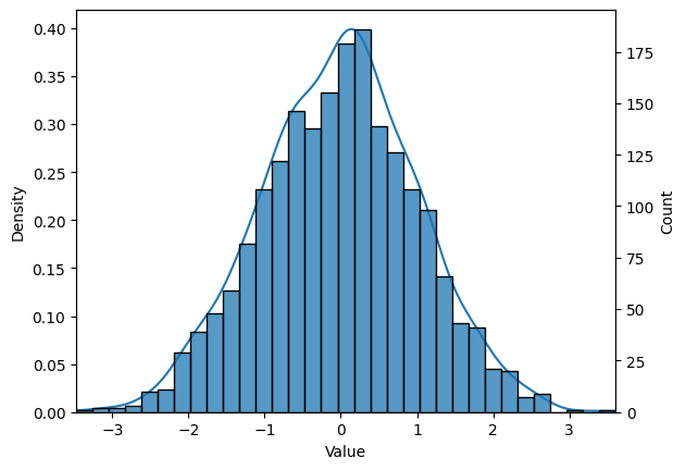
We generate a dataset of size $2000\times 2$ using the standard Gaussian distribution. One column is designated as the seed column and the other is watermarked. Figures 2(a) and 2(b) contain KDE plots showing minimal difference between the distribution before and after watermarking.

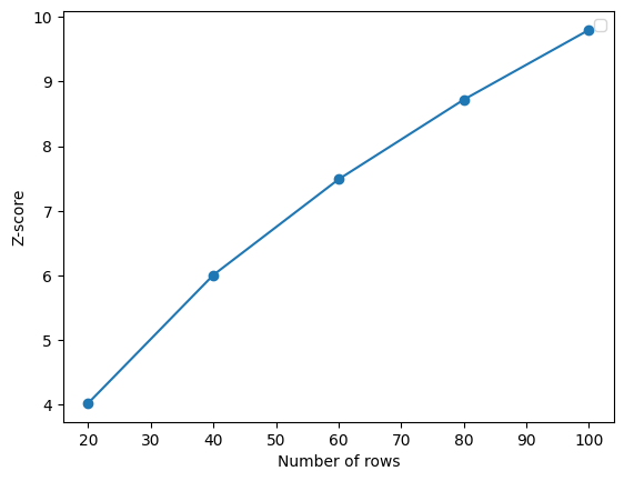
In the second experiment, we generate multiple datasets each containing 50 columns and varying numbers of rows from 20 to 100 in order to validate the effect that the row count has on the maximum achievable $z$ -score. We repeat this process 5 times and take the average $z$ -score. As shown in Figure 2(c), we find that as the number of rows in the dataset increases, so does the maximum possible $z$ -score. This means that given a choice of $z$ -score threshold, i) there is an increasing minimum number of total rows that the dataset must contain to achieve that score and ii) as the number of rows increases, so does the number of rows that an attacker must sufficiently alter to break the watermark.

Finally, we consider the fidelity vs. robustness trade off that the bin size parameter poses. We again generate a dataset of size $2000\times 2$ using the standard Gaussian distribution. We watermark one column, using the other for seeding, and vary the bin size between $10^{-4}$ and $10^{-1}$ . The average mean squared error across 5 runs between the original data and the watermarked data for each bin size is shown in Figure 2(d). As expected, greater fidelity is maintained with smaller bins since adjusting the data to fall into the nearest green bin requires smaller perturbations. Figure 2(e) displays the accompanying susceptibility to noise that comes with smaller bins. Averaging across 5 runs, we add zero-mean Gaussian noise with standard deviation varying from $10^{-3}$ to $10^{-1}$ to the watermarked data , and measure the effect on the $z$ -score. In each case, we find that smaller bins results in lower scores.

7.1.2 Classification

To validate the effectiveness of our feature importance based pairing scheme, we generate a multi-class classification dataset of size $75\times 75$ using scikit-learn, setting the number of classes to 5 and the number of informative features to 37. We create a set of column pairs using two different schemes: i) uniform: features are paired uniformly at random and ii) feature importance: sampling columns by treating their feature importances according to a Random Forest classifier as probabilities, pairing columns that are sampled one after the other. Using these two pairing schemes we create two watermarked datasets by watermarking 12 of the 37 available pairs, respectively.

For each of the watermarked datasets, we train a Random Forest classifier and use the resulting feature importances to drop subsets of columns varying in size from $20\%$ to $80\%$ . The metric of interest in this experiment is the percentage of pairs retained after column dropping. Both columns in a pair must still remain in the dataset to be counted as a preserved pair. This entire process is repeated 5 times, and the averaged results are shown in Figure 2(f). The results show there is a significant increase in preserved pairs when the pairs are created using the feature importance scheme.

7.2 Generative Tabular Data

7.2.1 Datasets and Generators

In a similar setup to He et al. [12], we evaluate our proposed watermarking technique using two real-world datasets of various sizes and distributions: Wilt [13], and California Housing Prices.

Wilt

This dataset is a public dataset that is part of the UCI Machine Learning Repository. It contains data from a remote sensing study that involved detecting diseased trees in satellite imagery. The data set consists of image segments, generated by segmenting the pansharpened image. The segments contain spectral information from the Quickbird multispectral image bands and texture information from the panchromatic (Pan) image band³³3Data available on the UCI platform at https://archive.ics.uci.edu/dataset/285/wilt. This dataset includes 4,889 records and 6 attributes.The attributes are a mixture of numerical and categorical data types. The data set has a binary target label which indicates whether a tree from is wilted or healthy. Therefore the dataset has a classification task which is to classify the tree samples as either diseased or healthy.

California Housing Prices

The dataset was collected from the 1990 U.S. Census and includes various socio-economic and geographical features that are believed to influence housing prices in a given California district. It contains 20,640 records and 10 attributes each of which represent data about homes in the district. Similar to the previous dataset, the attributes are a mixture of continuous and categorical data types. The dataset has a multi target label which indicates the proximity of each house to the ocean making it a multi-classification problem.

For each dataset, we generate corresponding synthetic datasets using neural network-based methods [22] and statistical-based generative methods [20]. Each of these methods for synthetic data generation possesses distinctive capabilities and features. For this paper, we employ CTGAN [29], Gaussian Copula [21], and TVAE [29] which represent GAN-based [10], copula-based [23], and VAE-based generators [17] respectively to generate tabular data.

7.2.2 Utility

Dataset

Method

Not WM

Watermarked (WM)

WM and Truncated

WM and

20% cols drop

WM and

40% cols drop

Random

California

CTGAN

0.373

0.371

0.368

0.301

0.242

0.203

0.256

Copula

0.370

0.376

0.347

0.332

0.31

0.30

TVAE

0.797

0.799

0.798

0.448

0.407

0.385

0.365

Wilt

CTGAN

0.731

0.733

0.575

0.574

0.563

Copula

0.99

0.996

0.995

0.994

0.993

TVAE

0.989

0.965

0.977

0.972

0.803

Table 2: Accuracy of the downstream models under various attacks to the watermarked datasets. In particular, we provide accuracy for the original dataset and its watermarked counterpart. Additionally, we consider truncation as well as the column dropping separately that are typical preprocessing steps in a machine learning pipeline. We note that the effect of our watermarking technique is negligible in terms of accuracy in all cases while maintaining high detectability.

For evaluating utility, we focus on machine learning (ML) efficiency [29]. In more detail, ML efficiency quantifies the performance of classification or regression models that are trained on synthetic data and evaluated on the real test set. In our experiment, we evaluate ML efficiency with respect to the XGBoost classifier [7] for classification tasks which are then evaluated on real testing sets. Classification performances are evaluated by the accuracy score. To explore the performance of our tabular watermark on real-world data, we sample from each generative model a generated dataset with the size of a real training set. For each setup, we create 5 watermarked training sets to measure the accuracy score. For reproducibility, we set a specific random seed to ensure that the data deformation and model training effects are repeatable on a similar hardware and software stack. To eliminate the randomness of the results, the experimental outcomes are averaged over multiple runs from each watermarked training set.

We watermark each of the generated datasets using a bin size of $10^{-2}$ and thus only consider columns that contain floating point numbers with at least 2 decimal places. This choice follows from the practical consideration that watermarking with this bin size involves perturbing up to 2 decimal places and watermarking any original columns that did not already contain values with this property may make it obvious to an outside party upon receiving the dataset that this specific section of the data has been manipulated.

We also consider two common data science preprocessing steps that downstream users of the watermarked datasets might conduct: truncation and dropping the least important columns. We aim to determine if the application of our watermark in conjunction with these operations For the former we truncate to 2 decimal places. For the latter we investigate dropping the lowest 20% and 40% of columns; in each case considering when the data is watermarked both with and without the feature importance based pairing scheme.

We find that the effect of our watermarking technique is negligible in terms of accuracy in all cases while maintaining high detectability as seen in Table 2.

8 Discussion and Future Work

In this work, we provided a novel robust watermarking scheme for tabular numerical datasets. Our watermarking method partitions the feature space into pairs of $(key,value)$ columns using knowledge of the feature importance in the downstream task. We use the center of the bins from each $key$ columns to generate randomized red and green intervals and watermark the $value$ columns by promoting its value to fall in green intervals. Compared to prior work in watermarking generative tabular data, our method is more robust to common preprocess attacks such as feature selection and truncation at the cost of harder detection. There are a few open questions in the current work that are ripe for investigation:

•

How do we include the categorical columns either in the key or the value of the watermarking process? Note that in the LLM setting, this was possible due to the richness of the vocabulary, which enabled replacing one token with a close enough token with similar semantic meaning.
•

Can we extend this framework to the LLM settings for tabular data generation? This extension will embed the watermark as part of the generation process [27] and the results in this paper will need to be adapted to the new setting. The samples generated by the LLM will be distorted due to the additional watermarking step and recent work [19] mitigates it by inducing correlations with secret keys. Similar injection of undetectable watermarks has been undertaken by Christ et al. [8]. Adapting these to our settings would be of great interest.
•

Can we provide an objective comparison between the strengths of the tabular watermarking schemes proposed by He et al. [12], Zheng et al. [30] and the current work? This comparison can be potentially accomplished by measuring the number of calls required to a watermark detector in order to break the watermarking scheme that has been employed.
•

The current watermark scheme only considers ’hard’ watermark, where all elements in the $value$ columns are deterministically placed in the nearest green intervals. Can we extend the current analysis to allow for a ’soft’ watermark scheme similar to the one described in Kirchenbauer et al. [18], where we first promote the probability of being in green intervals, then sample from such distribution to generate elements for the $value$ columns?

Disclaimer

This paper was prepared for informational purposes and is contributed by the Artificial Intelligence Research group of JPMorgan Chase & Co and its affiliates (“J.P. Morgan”), and is not a product of the Research Department of J.P. Morgan. J.P. Morgan makes no representation and warranty whatsoever and disclaims all liability, for the completeness, accuracy or reliability of the information contained herein. This document is not intended as investment research or investment advice, or a recommendation, offer or solicitation for the purchase or sale of any security, financial instrument, financial product or service, or to be used in any way for evaluating the merits of participating in any transaction, and shall not constitute a solicitation under any jurisdiction or to any person, if such solicitation under such jurisdiction or to such person would be unlawful.

References

Aaronson [2023] S. Aaronson. ‘Reform’ AI Alignment with Scott Aaronson. AXRP - the AI X-risk Research Podcast, 2023. URL https://axrp.net/episode/2023/04/11/episode-20-reform-ai-alignment-scott-aaronson.html.
Agrawal and Kiernan [2002] R. Agrawal and J. Kiernan. Watermarking relational databases. In VLDB’02: Proceedings of the 28th International Conference on Very Large Databases, pages 155–166. Elsevier, 2002.
An et al. [2024] B. An, M. Ding, T. Rabbani, A. Agrawal, Y. Xu, C. Deng, S. Zhu, A. Mohamed, Y. Wen, T. Goldstein, et al. Benchmarking the robustness of image watermarks. arXiv preprint arXiv:2401.08573, 2024.
Assefa et al. [2020] S. A. Assefa, D. Dervovic, M. Mahfouz, R. E. Tillman, P. Reddy, and M. Veloso. Generating synthetic data in finance: opportunities, challenges and pitfalls. In Proceedings of the First ACM International Conference on AI in Finance, pages 1–8, 2020.
Atallah et al. [2001] M. J. Atallah, V. Raskin, M. Crogan, C. Hempelmann, F. Kerschbaum, D. Mohamed, and S. Naik. Natural language watermarking: Design, analysis, and a proof-of-concept implementation. In Information Hiding: 4th International Workshop, IH 2001 Pittsburgh, PA, USA, April 25–27, 2001 Proceedings 4, pages 185–200. Springer, 2001.
Bonferroni [1936] C. Bonferroni. Teoria statistica delle classi e calcolo delle probabilita. Pubblicazioni del R istituto superiore di scienze economiche e commericiali di firenze, 8:3–62, 1936.
Chen and Guestrin [2016] T. Chen and C. Guestrin. Xgboost: A scalable tree boosting system. In Proceedings of the 22nd acm sigkdd international conference on knowledge discovery and data mining, pages 785–794, 2016.
Christ et al. [2023] M. Christ, S. Gunn, and O. Zamir. Undetectable watermarks for language models. arXiv preprint arXiv:2306.09194, 2023.
Gonzales et al. [2023] A. Gonzales, G. Guruswamy, and S. R. Smith. Synthetic data in health care: A narrative review. PLOS Digital Health, 2(1):e0000082, 2023.
Goodfellow et al. [2014] I. Goodfellow, J. Pouget-Abadie, M. Mirza, B. Xu, D. Warde-Farley, S. Ozair, A. Courville, and Y. Bengio. Generative adversarial nets. Advances in neural information processing systems, 27, 2014.
Hamadou et al. [2011] A. Hamadou, X. Sun, S. A. Shah, and L. Gao. A weight-based semi-fragile watermarking scheme for integrity verification of relational data. International Journal of Digital Content Technology and Its Applications, 5:148–157, 2011. URL https://api.semanticscholar.org/CorpusID:58278938.
He et al. [2024] H. He, P. Yu, J. Ren, Y. N. Wu, and G. Cheng. Watermarking generative tabular data, 2024. URL https://arxiv.org/abs/2405.14018.
Johnson [2014] B. Johnson. Wilt. UCI Machine Learning Repository, 2014. DOI: https://doi.org/10.24432/C5KS4M.
Jordon et al. [2022] J. Jordon, L. Szpruch, F. Houssiau, M. Bottarelli, G. Cherubin, C. Maple, S. N. Cohen, and A. Weller. Synthetic data-what, why and how? arXiv preprint arXiv:2205.03257, 2022.
Kamaruddin et al. [2018] N. S. Kamaruddin, A. Kamsin, L. Y. Por, and H. Rahman. A review of text watermarking: theory, methods, and applications. IEEE Access, 2018.
Katzenbeisser and Petitcolas [2000] S. Katzenbeisser and F. Petitcolas. Digital watermarking. Artech House, London, 2:2, 2000.
Kingma and Welling [2013] D. P. Kingma and M. Welling. Auto-encoding variational bayes. arXiv preprint arXiv:1312.6114, 2013.
Kirchenbauer et al. [2023] J. Kirchenbauer, J. Geiping, Y. Wen, J. Katz, I. Miers, and T. Goldstein. A watermark for large language models. arXiv preprint arXiv:2301.10226, 2023.
Kuditipudi et al. [2024] R. Kuditipudi, J. Thickstun, T. Hashimoto, and P. Liang. Robust distortion-free watermarks for language models. Transactions on Machine Learning Research, 2024. ISSN 2835-8856. URL https://openreview.net/forum?id=FpaCL1MO2C.
Li et al. [2020] Z. Li, Y. Zhao, and J. Fu. Sync: A copula based framework for generating synthetic data from aggregated sources. In 2020 International Conference on Data Mining Workshops (ICDMW), pages 571–578. IEEE, 2020.
Masarotto and Varin [2012] G. Masarotto and C. Varin. Gaussian copula marginal regression. Electronic Journal of Statistics, 6:1517–1549, 2012. URL https://api.semanticscholar.org/CorpusID:53962593.
Park et al. [2018] N. Park, M. Mohammadi, K. Gorde, S. Jajodia, H. Park, and Y. Kim. Data synthesis based on generative adversarial networks. arXiv preprint arXiv:1806.03384, 2018.
Patki et al. [2016] N. Patki, R. Wedge, and K. Veeramachaneni. The synthetic data vault. In 2016 IEEE international conference on data science and advanced analytics (DSAA), pages 399–410. IEEE, 2016.
Potluru et al. [2023] V. K. Potluru, D. Borrajo, A. Coletta, N. Dalmasso, Y. El-Laham, E. Fons, M. Ghassemi, S. Gopalakrishnan, V. Gosai, E. Kreačić, et al. Synthetic data applications in finance. arXiv preprint arXiv:2401.00081, 2023.
Shehab et al. [2007] M. Shehab, E. Bertino, and A. Ghafoor. Watermarking relational databases using optimization-based techniques. IEEE transactions on Knowledge and Data Engineering, 20(1):116–129, 2007.
Sion et al. [2003] R. Sion, M. Atallah, and S. Prabhakar. Rights protection for relational data. In Proceedings of the 2003 ACM SIGMOD International Conference on Management of Data, SIGMOD ’03, page 98–109, New York, NY, USA, 2003. Association for Computing Machinery. ISBN 158113634X. doi: 10.1145/872757.872772. URL https://doi.org/10.1145/872757.872772.
Venugopal et al. [2011] A. Venugopal, J. Uszkoreit, D. Talbot, F. J. Och, and J. Ganitkevitch. Watermarking the outputs of structured prediction with an application in statistical machine translation. In Proceedings of Empirical Methods for Natural Language Processing, 2011.
Xiao et al. [2007] X. Xiao, X. Sun, and M. Chen. Second-lsb-dependent robust watermarking for relational database. In Third International Symposium on Information Assurance and Security, pages 292–300, 2007. doi: 10.1109/IAS.2007.25.
Xu et al. [2019] L. Xu, M. Skoularidou, A. Cuesta-Infante, and K. Veeramachaneni. Modeling tabular data using conditional gan. Advances in neural information processing systems, 32, 2019.
Zheng et al. [2024] Y. Zheng, H. Xia, J. Pang, J. Liu, K. Ren, L. Chu, Y. Cao, and L. Xiong. Tabularmark: Watermarking tabular datasets for machine learning, 2024. URL https://arxiv.org/abs/2406.14841.

Appendix A Proof of Fidelity

Proofs of Equation 1

Proof.

Observe that the watermarked dataset $\mathbf{X}_{w}$ only differs from the original dataset $\mathbf{X}$ in the $value$ columns. For each element $x$ in the $value$ column of the original dataset $\mathbf{X}$ , let $Y$ denote the chosen nearest interval from the green list. Then, we have

	$\displaystyle\mathbb{E}[\left\lvert x-x_{w}\right\rvert]$
	$\displaystyle\leq\max_{y\in Y}\mathbb{E}[\left\lvert x-y\right\rvert]$
	$\displaystyle\leq\max_{y\in Y}\mathbb{E}\left[\left\lvert x-y\right\rvert\Big{\|}\left\lvert x-y\right\rvert\leq\frac{k}{b}\right]\cdot\Pr\left[\left\lvert x-y\right\rvert\leq\frac{k}{b}\right]$
	$\displaystyle\qquad+\mathbb{E}\left[\left\lvert x-y\right\rvert\Big{\|}\left\lvert x-y\right\rvert>\frac{k}{b}\right]\cdot\Pr\left[\left\lvert x-y\right\rvert>\frac{k}{b}\right]$
	$\displaystyle\leq\max_{y\in Y}\frac{k}{b}\cdot\left(1-\frac{1}{2^{k}}\right)+1\cdot\frac{1}{2^{k}}$
	$\displaystyle=\frac{k(2^{k}-1)}{b\cdot 2^{k}}+\frac{1}{2^{k}}$
	$\displaystyle=\frac{k\cdot(2^{k}-1)+2b}{b\cdot 2^{k}}$

where $k\in[1,b)$ is a random variable denoting the search radius for the nearest green interval. Then, choosing $\delta=\frac{1}{2^{k}}$ , we have with probability at least $1-\delta$ :

\displaystyle\mathbb{E}[\left\lVert\mathbf{X}-\mathbf{X}_{w}\right\rVert_{\infty}]\leq\frac{\log_{2}(1/\delta)}{b}

∎

Proof of Corollary 4.2

Proof.

By definition of $k$ -Wasserstein distance, we have with probability at least $1-\delta$ for $\delta\in(0,1)$ :

	$\displaystyle\mathcal{W}_{k}(F_{\mathbf{X}},F_{\mathbf{X}_{w}})$
	$\displaystyle\leq\left(\sum_{j=1}^{m}\frac{1}{m}\left\lVert\mathbf{X}[j,:]-\mathbf{X}_{w}[j,:]\right\rVert_{2}^{k}\right)^{1/k}$
	$\displaystyle\leq\left(\sum_{j=1}^{m}\frac{1}{m}\left(\sqrt{2n}\left\lVert\mathbf{X}[j,:]-\mathbf{X}_{w}[j,:]\right\rVert_{\infty}\right)^{k}\right)^{1/k}$
	$\displaystyle\leq\left(\sum_{j=1}^{m}\frac{1}{m}\left(\sqrt{2n}\cdot\frac{\log_{2}(1/\delta)}{b}\right)^{k}\right)^{1/k}$
	$\displaystyle=\left(\sum_{j=1}^{m}\frac{1}{m}\frac{(\sqrt{2n}\cdot\log_{2}(1/\delta))^{k}}{b^{k}}\right)^{1/k}$
	$\displaystyle=\frac{\sqrt{2n}\cdot\log_{2}(1/\delta)}{b}$

∎

Appendix B Proofs of Detectability

Proof of Lemma 5.1

Proof.

Let $I_{j}=\left[\frac{j-1}{b},\frac{j}{b}\right]$ denote an interval on $[0,1]$ . Then, for each element $x$ in a $value$ column, we have:

	$\displaystyle\Pr_{x\sim F}[x\in G]$	$\displaystyle=\Pr_{x\sim F}[\bigcup_{j=1}^{b}\{x\in I_{j}\&I_{j}\in G\}]$
		$\displaystyle=\sum_{j=1}^{b}\Pr_{x\sim F}[x\in I_{j}\&I_{j}\in G]$
		$\displaystyle=\sum_{j=1}^{b}\Pr[x\in I_{j}\|I_{j}\in G]\cdot\Pr[I_{j}\in G]$
		$\displaystyle=\sum_{j=1}^{b}\Pr[x\in I_{j}]\cdot\frac{1}{2}$
		$\displaystyle=\frac{1}{2}$

∎

Appendix C Proofs of Robustness

Proof of Theorem 6.2

Proof.

We first look at the number of preserved columns under uniform pairing.

Uniform pairing.

Let $\mathbf{X}^{\prime}_{w}\in[0,1]^{m\times k}$ denote the watermarked dataset after feature selection.

Consider the set of all possible pairs of columns after feature selection can be matched together. Then, there are $\binom{k}{2}$ possible choices, which are the number of $2$ -subset from $k$ total columns. Define an event $Y_{\ell}=\mathbf{1}[\ell\text{-th subset is a pair}]$ . In each $2$ -subset, after a first column is selected, the probability that the second column actually forms a pair with the first column is $\nicefrac{{1}}{{2n-1}}$ . Hence, we have:

\displaystyle\mathbb{E}[Y_{\ell}]=\frac{1}{2n-1}

Hence, the expected number of preserved pairs of columns in $\mathbf{X}^{\prime}_{w}$ under uniform random pairing can be obtained by summing over all $\binom{k}{2}$ possible choices as follow.

	$\displaystyle\quad\mathbb{E}[\text{number of preserved pairs}\in\mathbf{X}^{\prime}_{w}]$
	$\displaystyle=\sum_{\ell=1}^{\binom{k}{2}}\mathbb{E}[Y_{\ell}]$
	$\displaystyle=\binom{k}{2}\frac{1}{2n-1}$
	$\displaystyle=\frac{(k-1)k}{2(2n-1)}$

Now, we can look at the number of preserved pairs of columns under feature importance pairing. Note that we assume the feature selection is performed according to 6.1, and the columns are in descending order of feature importance. Since we are only retaining the top $k$ most important features after feature selection, this is equivalent to counting the number of preserved pairs among the first $k$ features after reordering.

Feature importance pairing.

When the columns are paired according to the feature importance ordering, we match them according to Equation 4. Define the event $Y_{i,j}=\mathbf{1}[\text{columns }(i,j)\text{ is a pair}]$ . Then, for fixed columns $i$ and $j$ , we have:

	$\displaystyle\mathbb{E}[Y_{\ell}]$	$\displaystyle=\frac{\frac{1}{\left\lvert i-j\right\rvert}}{\sum_{j\neq i}^{2n}\frac{1}{\left\lvert i-\ell\right\rvert}}$
		$\displaystyle=\frac{\frac{1}{\left\lvert i-j\right\rvert}}{\sum_{\ell=1}^{i-1}\frac{1}{\ell}+\sum_{s=1}^{2n-i}\frac{1}{s}}$
		$\displaystyle=\frac{\frac{1}{\left\lvert i-j\right\rvert}}{H_{i-1}+H_{2n-i}}$

where $H_{i}$ is the $i$ -th harmonic number. We know that for $i\geq 1$ , we have $\ln(i+1)\leq H_{i}\leq\ln(i)+1$ . Let $\Delta_{i}=\max\{i-1,2n-i\}$ . Since only the top-k columns are retained, we have:

	$\displaystyle\mathbb{E}[\text{number of preserved pairs}\in\mathbf{X}^{\prime}_{w}]$
	$\displaystyle=\sum_{i=1}^{k}\sum_{j\neq i,j=1}^{k}\frac{1}{\left\lvert i-j\right\rvert(H_{i-1}+H_{2n-i})}$
	$\displaystyle=\sum_{i=1}^{k}\frac{1}{H_{i-1}+H_{2n-i}}\left(\sum_{j\neq i,j=1}\frac{1}{\left\lvert i-j\right\rvert}\right)$
	$\displaystyle=\sum_{i=1}^{k}\frac{1}{H_{i-1}+H_{2n-i}}\left(H_{i-1}+H_{k-i}\right)$
	$\displaystyle=\sum_{i=1}^{k}1-\frac{H_{2n-i}-H_{k-i}}{H_{i-1}+H_{2n-i}}$
	$\displaystyle=k-\sum_{i=1}^{k}\frac{H_{2n-i}-H_{k-i}}{H_{i-1}+H_{2n-i}}$
	$\displaystyle\geq k-\sum_{i=1}^{k}\frac{H_{2n-i}}{H_{i-1}+H_{2n-i}}$

Since we assume that $k<n$ , we have

	$\displaystyle i<n$	$\displaystyle\Rightarrow 2n-i>n>i-1$
		$\displaystyle\Rightarrow\frac{1}{i-1}>\frac{1}{2n-i}$
		$\displaystyle\Rightarrow H_{i-1}<H_{2n-i}$
		$\displaystyle\Rightarrow\frac{H_{2n-i}}{H_{i-1}+H_{2n-i}}>\frac{1}{2}$

Therefore, the expected number of preserved pairs under feature importance pairing is $\nicefrac{{k}}{{2}}$ .

Finally, we can compare the number of preserved pairs under the two pairing schemes:

	$\displaystyle\frac{\frac{k}{2}}{\frac{(k-1)k}{2(2n-1)}}$	$\displaystyle=\frac{k}{2}\frac{2(2n-1)}{(k-1)k}$
		$\displaystyle=\frac{2n-1}{k-1}$
		$\displaystyle\geq\frac{2k-1}{k-1}$
		$\displaystyle>\frac{2k-2}{k-1}$
		$\displaystyle=2$

Therefore, we retain twice as many pairs of $(key,value)$ columns by using feature importance pairing scheme compared to the naive approach of uniformly random pairing. ∎

Proof of Theorem 6.3

Proof.

If $x_{\mathrm{tr}}$ falls out of the original green interval $I_{j}$ , then we know that either $x_{\mathrm{tr}}>\nicefrac{{j}}{{b}}$ or $x_{\mathrm{tr}}<\nicefrac{{j-1}}{{b}}$ . Since $b\leq 10^{p}$ , we know that the green interval $I_{j}$ lies in the union of at most two consecutive grids. We consider two cases depending on whether $I_{j}$ contains a grid point or not.

When $I_{j}$ does not contain a grid point.

Since the truncation function defined in Equation 5 always truncate an element $x$ to the nearest left grid point, which lies outside of $I_{j}$ , we have

\Pr\left[x_{\mathrm{tr}}\notin I_{j}|c\notin I_{j},\forall c\in\text{grid}\right]=1.

When $I_{j}$ contains a grid point.

Let $c$ denote the grid point in $I_{j}$ . Then, when the interval $I_{j}$ contains a grid point, we have:

	$\displaystyle\Pr[x_{\mathrm{tr}}\notin I_{j}\|c\in I_{j}]$	$\displaystyle=\Pr\left[x\in\Big{[}\frac{j-1}{b},c\Big{)}\right]$
		$\displaystyle=\frac{c-\frac{j-1}{b}}{\frac{1}{b}}$
		$\displaystyle=c\cdot b-j+1$

Then, summing over all possible events, we have the probability that the truncation attack successfully moves a watermarked element out of its original green interval is:

	$\displaystyle\quad\Pr[x_{\mathrm{tr}}\notin I_{j}]$
	$\displaystyle=\Pr[x_{\mathrm{tr}}\notin I_{j}\|c\notin I_{j},\forall c\in\text{grid}]\cdot\Pr[c\notin I_{j},\forall i\in\text{grid}]$
	$\displaystyle+\Pr[x_{\mathrm{tr}}\notin I_{j}\|c\in I_{j}]\cdot\Pr[c\in I_{j}]$
	$\displaystyle=\Pr[c\notin I_{j},\forall c\in\text{grid}]+(c\cdot b-j+1)\Pr[c\in I_{j}]$
	$\displaystyle=\left(\frac{b-1}{b}\right)^{10^{p}}+\frac{c\cdot b-j+1}{b}$
	$\displaystyle=\frac{(b-1)^{10^{p}}+b^{10^{p}-1}(c\cdot b-j+1)}{b^{10^{p}}}$

∎

Appendix D Additional experiments

D.1 Standard deviation

To investigate the performance of our tabular watermark on real-world data, we sample from each generative model a generated dataset. For each setup, we create 5 watermarked training sets of each generator so as to measure the mean accuracy and standard deviation. We use XGBoost classifier and Random Forest classifier for classification tasks which are then evaluated on real testing sets.

Dataset

Method

Not WM

Watermarked (WM)

WM and Truncated

WM and

40% cols drop

Random

California

CTGAN

0.373\pm 0.019

0.371\pm 0.012

0.368\pm 0.013

0.203\pm 0.13

0.256\pm 0.054

Copula

0.371\pm 0.024

0.376\pm 0.025

0.376\pm 0.032

0.31\pm 0.1

0.30\pm 0.13

TVAE

0.797\pm 0.018

0.799\pm 0.023

0.798\pm 0.020

0.385\pm 0.192

0.365\pm 0.077

Wilt

CTGAN

0.731\pm 0.033

0.733\pm 0.041

0.733\pm 0.041

0.563\pm 0.034

0.563\pm 0.031

Copula

0.99\pm 0.012

0.996\pm 0.013

0.996\pm 0.012

0.993\pm 0.017

0.993\pm 0.017

TVAE

0.989\pm 0.001

0.989\pm 0.001

0.989\pm 0.002

0.972\pm 0.041

0.803\pm 0.01

Table 3: Accuracy of the downstream models under various attacks to the watermarked datasets. In particular, we provide accuracy for the original dataset and its watermarked counterpart. Classifier used for utility evaluation is XGBoost. In addition to this, we add the standard deviation of each record.

Dataset

Method

Not WM

Watermarked (WM)

WM and Truncated

WM and

40% cols drop

Random

California

CTGAN

0.379\pm 0.014

0.379\pm 0.011

0.382\pm 0.011

0.309\pm 0.126

0.334\pm 0.124

Copula

0.377\pm 0.024

0.393\pm 0.025

0.393\pm 0.026

0.278\pm 0.18

0.333\pm 0.069

TVAE

0.805\pm 0.021

0.809\pm 0.024

0.808\pm 0.019

0.399\pm 0.185

0.449\pm 0.183

Wilt

CTGAN

0.849\pm 0.037

0.856\pm 0.035

0.859\pm 0.036

0.644\pm 0.403

0.617\pm 0.420

Copula

0.986\pm 0.011

0.986\pm 0.012

0.985\pm 0.012

0.973\pm 0.015

0.969\pm 0.017

TVAE

0.985\pm 0.001

0.985\pm 0.001

0.985\pm 0.001

0.985\pm 0.001

0.81\pm 0.397

Table 4: Accuracy of the downstream models under various attacks to the watermarked datasets. In particular, we provide accuracy for the original dataset and its watermarked counterpart. Classifier used for utility evaluation is Random Forest. In addition to this, we add the standard deviation of each record.

D.2 Detection computation

We further investigate the effects that algorithm parameters and downstream manipulations have on the robustness and computational requirements of the detection mechanism. We measure the number of column pairing tests that must be done before a high confidence pair is found. We define high confidence as achieving a $z$ -score of 4 using 24 randomly selected rows. The process is stopped early when the watermark is detected. Thus, when a watermark cannot be found, the result becomes $N^{2}-N$ , where $N$ is the number of columns in the dataset.

We compare non-watermarked and watermarked data, and also test with truncation and dropped columns as before. For the latter, here, we compare the 4 total combinations of column ordering choices: watermarking and detection both present the option to order by feature importance or to order randomly. We find that, with truncation, it generally takes the same number of computations as without and that this amount is significantly lower than the upper bound in the "Not watermarked" column.

Dataset	Method	Not watermarked	Watermarked	Watermarked & truncated
California	CTGAN	$72\pm 0$	$16\pm 0$	$19.6\pm 4.41$
	Copula	$72\pm 0$	$16\pm 0$	$30\pm 4.94$
	TVAE	$72\pm 0$	$58.6\pm 11.11$	$58.4\pm 11.35$
Wilt	CTGAN	$20\pm 0$	$9.2\pm 4.62$	$9.2\pm 4.62$
	Copula	$20\pm 0$	$5.4\pm 3.5$	$5.6\pm 3.38$
	TVAE	$20\pm 0$	$2.4\pm 0.5$	$2.2\pm 0.4$

Table 5: Number of column pair tests executed during detection process. The process is stopped early when the watermark is detected. Thus, when a watermark cannot be found, the result becomes

N^{2}-N

, where

N

is the number of columns in the dataset.

Appendix E Settings of Experiments

E.1 Specifications

For synthetic data generation using three generative methods mentioned in the paper, we follow the default hyperparameters found in the SDV library [23]. We run the experiments on a machine type of g4dn.4xlarge consisting of 16 CPU, 64GB RAM, and 1 GPU. For Utility evaluation, default parameters of the XGBoost classifier [7] and Random Forest classifier with a seed of 42 was used. The synthetic data generation, training and evaluation process typically finishes within 4 hrs. Python 3.8 version was used to run the experiments.

Adaptive and Robust Watermark for Generative Tabular Data

Abstract

1 Introduction

2 Related Work

Watermarking tabular data

3 Problem Formulation

Notation.

4 Pairwise Tabular Data Watermark

4.1 Fidelity of Pairwise Tabular Data Watermark

Theorem 4.1 (Fidelity).

Corollary 4.2 (Wasserstein distance).

5 Detection of Pairwise Tabular Data Watermark

Lemma 5.1.

Hypothesis test

6 Robustness of Pairwise Tabular Data Watermark

6.1 Robustness to Feature Selection

Assumption 6.1.

Theorem 6.2.

6.2 Robustness to Truncation

Theorem 6.3.

7 Experiments

7.1 Synthetic Tabular Data

7.1.1 Gaussian data

7.1.2 Classification

7.2 Generative Tabular Data

7.2.1 Datasets and Generators

Wilt

California Housing Prices

7.2.2 Utility

8 Discussion and Future Work

Disclaimer

References

Appendix A Proof of Fidelity

Proofs of Equation 1

Proof.

Proof of Corollary 4.2

Proof.

Appendix B Proofs of Detectability

Proof of Lemma 5.1

Proof.

Appendix C Proofs of Robustness

Proof of Theorem 6.2

Proof.

Uniform pairing.

Feature importance pairing.

Proof of Theorem 6.3

Proof.

When IjI_{j} does not contain a grid point.

When IjI_{j} contains a grid point.

Appendix D Additional experiments

D.1 Standard deviation

D.2 Detection computation

Appendix E Settings of Experiments

E.1 Specifications

When $I_{j}$ does not contain a grid point.

When $I_{j}$ contains a grid point.