Adaptive and Efficient Learning with Blockwise Missing and Semi-Supervised Data

Data fusion enables more powerful and comprehensive analysis by integrating complementary views provided by different data sources, and has been more and more frequently adopted with the increasing capacity in unifying and synthesizing data models across different cohorts or institutions. As an important example, in the field of health and medicine, there has been growing interests and efforts in linking electronic medical records (EMRs) with biobank data to tackle complex health issues (Bycroft et al.,, 2018; Castro et al.,, 2022, e.g.). EMRs include detailed longitudinal clinical observations of patients, offering a rich source of health information over time. By combining these records with the genetics, genomics and other multi-omics data in biobanks, this type of data fusion enables a much deeper understanding of disease prognosis at the molecular level, potentially transforming patient care and treatment strategies (Zengini et al.,, 2018; Verma et al.,, 2023; Wang et al.,, 2024, e.g.). In addition to combine different types of data, data fusion has also been scaled up to merge data from multiple institutions. The UK Biobank (Sudlow et al.,, 2015) and the All-of-Us Research Program (The All of Us Research Program Investigators,, 2019) in the U.S. are prime examples.

To robustly and efficiently learn from multi-source fused data sets, several main statistical challenges need to be addressed. One is blockwise missing (BM) often occurring when certain variables are collected or defined differently across the sources. Consequently, one or multiple entire blocks of covariates are missing in the merged dataset. Dealing with the paucity of accurate outcomes in EMR is another major problem. This is due to the intensive human efforts or time costs demanded for collecting accurate outcomes like the manual chart reviewing labels created by experts for certain diseases or a long-term endpoint taking years to follow on. In this situation, one is often interested in semi-supervised (SS) learning that combines some small labeled subset with the large unlabeled sample collected from the same population without observations of the true outcome. In the aforementioned EMR applications, it is often to have the BM and SS problems occurring together, e.g., our real example in Section 5. This new setup has a more complicated data structure to be formally described in Section 1.2 and motivates our methodological research in this paper.

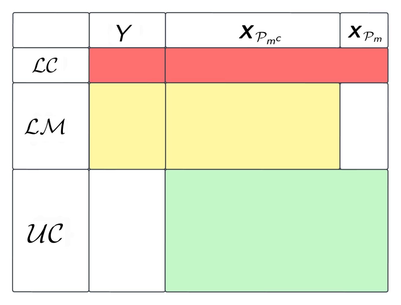
Let $Y$ be the outcome of interest and $\boldsymbol{X}=(X_{1},X_{2},...,X_{p})^{\top}$ be a vector of $p$-dimensional covariates. As illustrated on the left panel of Figure 1, there are three data structures of the observations from the same population: (i) $N_{\mathcal{L}\mathcal{C}}$ observations of $(Y,\boldsymbol{X})$ that are labeled and complete, denoted as $\mathcal{L}\mathcal{C}$; (ii) $N_{\mathcal{L}\mathcal{M}}$ labeled and covariates-missing observations of $(Y,\boldsymbol{X}_{\mathcal{P}_{m^{c}}})$ denoted as $\mathcal{L}\mathcal{M}$ where $\mathcal{P}_{m}\subset\{1,2,\ldots,p\}$ is the index set of the blockwise missing covariates and $\mathcal{P}_{m^{c}}=\{1,2,...,p\}\setminus\mathcal{P}_{m}$; and (iii) $N_{\mathcal{U}\mathcal{C}}$ unlabeled sample with complete observation of the covariates denoted as $\mathcal{U}\mathcal{C}$. Note that we consider a missing completely at random (MCAR) regime with the $\mathcal{L}\mathcal{C}$, $\mathcal{L}\mathcal{M}$ and $\mathcal{U}\mathcal{C}$ samples having a homogeneous underlying distribution. In the SS setting, we assume that $N_{\mathcal{U}\mathcal{C}}\gg N_{\mathcal{L}\mathcal{C}}+N_{\mathcal{L}\mathcal{M}}$. Denote by $\rho={N_{\mathcal{L}\mathcal{M}}}/{N_{\mathcal{L}\mathcal{C}}}$. In our application, $N_{\mathcal{L}\mathcal{C}}$ and $N_{\mathcal{L}\mathcal{M}}$ have similar magnitudes while our method and theory also accommodate the $\rho\rightarrow 0$ and $\rho\rightarrow\infty$ scenarios. Let $N=N_{\mathcal{L}\mathcal{C}}+N_{\mathcal{U}\mathcal{C}}+N_{\mathcal{L}\mathcal{M}}$, and the observed samples as

where $\mathcal{T}_{i}\in\{\mathcal{L}\mathcal{C},\mathcal{U}\mathcal{C},\mathcal{L}\mathcal{M}\}$ indicates the data type of the observation $i$. Also, we are interested the scenario with multiple BM structures: $\mathcal{T}_{i}\in\{\mathcal{L}\mathcal{C},\mathcal{U}\mathcal{C},\mathcal{L}\mathcal{M}_{1},\ldots,\mathcal{L}\mathcal{M}_{R}\}$ with each $\mathcal{L}\mathcal{M}_{r}$ representing a subset of data with observations of $(Y,\boldsymbol{X}_{\mathcal{P}_{m^{c}}^{r}})$ and missing covariates on the index set $\mathcal{P}_{m}^{r}$ satisfying $\mathcal{P}_{m}^{r}\neq\mathcal{P}_{m}^{\ell}$ for any pair of $r\neq\ell$ in $\{1,\ldots,R\}$; see the right panel of Figure 1.

Our primary interest lies in estimating and inferring the generalized linear model (GLM):

where $\boldsymbol{\gamma}=(\gamma_{1},\gamma_{2},...,\gamma_{p})^{\top}$ is a vector of unknown coefficients and $g(\cdot)$ is a known link function. For example, $g(a)=a$ corresponds to the Gaussian linear model and $g(a)=e^{a}/(1+e^{a})$ for the logistic model. It is important to note that our framework allows the model (1) to be misspecified, and we actually define the model coefficients of our interests as $\bar{\boldsymbol{\gamma}}$, the solution to the population-level moment equation:

The model parameter $\boldsymbol{\gamma}=(\gamma_{1},\ldots,\gamma_{p})^{\top}$ can be identified and estimated using the standard regression on the $\mathcal{L}\mathcal{C}$ sample but $\mathcal{L}\mathcal{M}$ and $\mathcal{U}\mathcal{C}$ cannot be directly incorporated into this procedure, which results in loss of effective samples. In this paper, our aim is to leverage both the $\mathcal{L}\mathcal{M}$ and $\mathcal{U}\mathcal{C}$ samples to enhance the estimation efficiency of $\boldsymbol{\gamma}$ without incurring bias. As will be introduced in Section 5.1, the data in our setup can also include auxiliary features that are predictive of $Y$ and $\boldsymbol{X}$, observed on all subjects, and possibly high-dimensional. These variables are not included in the outcome model $Y\sim\boldsymbol{X}$ of our primary interest due to scientific reasons but can be simply incorporated into our framework to enhance estimation efficiency. For the ease of presentation, we drop the notation of such auxiliary features in the main body of our method and theory.

With the increasing ability in collecting data with common models across multiple institutions, integrative regression with blockwise missing covariates has been an important problem frequently studied in recent literature. One of the most well known and commonly used approach to address missing data is Multiple Imputation with Chained Equations (MICE) White et al., (2011). However, as a practical, general, and principal strategy, MICE is sometimes subjected to high computation costs as well as potential bias and inefficiency caused by the misspecification or excessive error in imputation, e.g., see our simulation results.

Recently, Yu et al., (2020) proposed an approach named DISCOM for integrative linear regression under BM. It approximates the covariance of $(\boldsymbol{X},Y)$ through the optimal linear combination across different data structures and incorporates it with an extended sparse regression to derive an integrative estimator. Xue and Qu, (2021) proposed a multiple blockwise imputation (MBI) approach that aggregates linear estimating equations with multi-source imputed data sets constructed according to their specific BM structures. They justified the efficiency gain of their proposal over the complete-data-only estimator. Xue et al., (2021) extended this framework work for high-dimensional inference with BM data sets. Inspired by the idea of debiasing, Song et al., (2024) developed an approach for a similar problem without imputing the missing blocks but showing better efficiency. Jin and Rothenhäusler, (2023) proposed a modular regression approach accommodating BM covariates under the conditional independence assumption across the blocks of covariates given the response.

All works reviewed above primarily focused on the linear model, which is subtly different from the GLM with a nonlinear link as the latter typically requires the $\mathcal{L}\mathcal{C}$ sample to ensure identifiability of the outcome model while the linear model does not. For integrative GLM regression with BM data, Li et al., 2023b proposed a penalized estimating equation approach with multiple imputation (PEE–MI) that incorporates the correlation of multiple imputed observations into the objective function and realizes effective variable selection. Kundu and Chatterjee, (2023) and Zhao et al., (2023) proposed to incorporate the $\mathcal{L}\mathcal{M}$ sample through the generalized methods of moments (GMM) that actually uses the score functions of a reduced GLM (i.e., the parametric GLM for $Y\sim\boldsymbol{X}_{\mathcal{P}_{m^{c}}}$) on the $\mathcal{L}\mathcal{M}$ sample for variance reduction. Such a “reduced model” strategy has been used frequently in other work like Song et al., (2024), as well as for fusing clinical and observational data to enhance the efficiency of causal inference (Yang and Ding,, 2019; Hatt et al.,, 2022; Shi et al.,, 2023, e.g.).

As will be detailed in our asymptotic and numerical studies, the above-introduced reduced model or imputation strategies does not characterize the true influence of the $\mathcal{L}\mathcal{M}$ data and, thus, not achieving semiparametric efficiency in the BM regression setting, which dates back to the seminal work by Robins et al., (1994) and has been explored (Chen et al.,, 2008; Li and Luedtke,, 2023; Li et al., 2023a, ; Qiu et al.,, 2023, e.g.) in various settings. In particular, Li and Luedtke, (2023) proposed derived the canonical gradient for a general data fusion problem and justified its efficient. Nevertheless, such semiparametric efficiency property is established under an ideal scenario with a correct conditional model for $\boldsymbol{X}_{\mathcal{P}_{m}}$, which is stringent in practice. Their method could be less robust and effective in a more realistic case when the imputation for $\boldsymbol{X}_{\mathcal{P}_{m}}$ is not consistent with the truth. This issue has been recognized and studied in recent literature mainly focusing on SS inference (Gronsbell et al.,, 2022; Schmutz et al.,, 2022; Song et al.,, 2023; Angelopoulos et al.,, 2023; Miao et al.,, 2023; Gan and Liang,, 2023; Wu and Liu,, 2023). Notably, in our real-world study including high-dimensional auxiliary features to impute the missing variables (see Section 5.1), this problem is even more pronounced due to the difficulty of high-dimensional modeling. In this case, it is challenging to realize adaptive and efficient data fusion with above-mentioned strategies, which can be seen from the results in Section 5.

Our work is also closely related to recent progress in semi-supervised learning (SSL) that aims at using the large unlabeled sample to enhance the statistical efficiency of the analysis with relatively small labeled data sets. On this track, Kawakita and Kanamori, (2013) and Song et al., (2023) proposed to use some density ratio model matching the labeled and unlabeled samples to reweight the regression on the labeled sample, which, counter-intuitively, results in SSL estimators with smaller variances than their supervised learning (SL) counterparts. Chakrabortty and Cai, (2018) and Gronsbell et al., (2022) proposed to incorporate the unlabeled sample by imputing its unobserved outcome $Y$ with an imputation model constructed with the labeled data. Extending this imputation framework, Cai and Guo, (2020), Zhang and Bradic, (2022) and Deng et al., (2023) studied the SSL problem with high-dimensional $\boldsymbol{X}$, and Wu and Liu, (2023) addressed the SSL of graphic models.

Though having different constructions, these recent SSL approaches achieve a very similar adaptive property that they can produce SSL estimators more efficient than SL when the outcome model for $\mathrm{E}(Y|\boldsymbol{X})$ is misspecified and as efficient as SL when it is correct. Azriel et al., (2022) discussed this property and realized it for linear models in a more flexible and effective way. Notably, our SSL setting with BM designs has not been studied in this track of SSL literature. As will be shown later, this problem is essentially distinguished from existing work in SSL as the efficiency gain by using the $\mathcal{U}\mathcal{C}$ sample is attainable even when the outcome model (1) is correctly specified in our case. In addition, we notice that Xue et al., (2021) and Song et al., (2024) also considered using large $\mathcal{U}\mathcal{C}$ samples to assist learning of high-dimensional linear models under the BM setting. Unlike us, they only used the $\mathcal{U}\mathcal{C}$ sample to combat and reduce the excessive regularization errors in sparse regression and debiased inference. Nevertheless, for the inference of a low-dimensional projection of the model parameters, the asymptotic variance still remains unchanged compared to the SL scenario after incorporating the $\mathcal{U}\mathcal{C}$ sample in their methods.

Regarding the limitation of existing work discussed in the previous section, we propose a Data-adaptive projecting Estimation approach for data FUsion in the SEmi-supervised setting (DEFUSE). Our method contains two major novel steps, it initiates from the simple $\mathcal{L}\mathcal{C}$-only estimator, and first incorporates the $\mathcal{L}\mathcal{M}$ sample to reduce its asymptotic variance through a data-adaptive projection procedure for the score functions. Then, it utilizes the large $\mathcal{U}\mathcal{C}$ sample in another projecting step, to further improve the efficiency of the data-fused estimator resulting from the previous step. In the following, we shall summarize the main novelty and contribution of our work that have been justified and demonstrated through the asymptotic, simulation, and real-world studies.

1. 1.

   Our approach in combining the $\mathcal{L}\mathcal{M}$ and $\mathcal{L}\mathcal{C}$ samples is shown to produce an asymptotically unbiased and more efficient estimator compared to recent developments for BM regression (Xue and Qu,, 2021; Zhao et al.,, 2023; Song et al.,, 2024, e.g.). The newly proposed framework is inspired by the semiparametric theory and allows the flexible use of general ML algorithms to impute the missing variables. The efficiency gain of our method over existing methods in various settings like model misspecification are justified from both the theoretical and numerical perspectives.

2. 2.

   We develop a novel data-driven control function approach to realize adaptive and efficient estimation under potential misspecification or poor quality of the imputation models, especially when there exists nonlinear relationship not captured by them. Compared to recent work in addressing problematic nuisance models (Angelopoulos et al.,, 2023; Miao et al.,, 2023, e.g.), our strategy is shown to realize more flexible and efficient calibration in our theory, simulation, and real-world studies. This improvement is even clearer when high-dimensional auxiliary features are included in the nuisance model like our EMR application.

3. 3.

   We establish a novel framework to bring in large unlabeled samples under the SS setting and leverage them to enhance the efficiency of the BM estimation. This enables a more efficient use of the $\mathcal{U}\mathcal{C}$ sample leading to an estimator of strictly smaller variance than that obtained only using $\mathcal{L}\mathcal{C}$ and $\mathcal{L}\mathcal{M}$, which has not been readily achieved in previous work on a similar setting (Xue et al.,, 2021; Song et al.,, 2024). Our development is also shown to be more efficient than existing approaches for the standard SS setting without BM (Gronsbell et al.,, 2022, e.g.), in both theoretical and numerical studies.

4. 4.

   We propose a linear allocation approach to extend our framework in addressing multiple BM structures, in which the classic semiparametric theory does not apply.

Without the loss of generality, we aim at estimating and inferring a linear projection of the model coefficients $\boldsymbol{\gamma}$ denoted by $\boldsymbol{c}^{\top}\boldsymbol{\gamma}$ where $\boldsymbol{c}$ is an arbitrary vector satisfying $\|\boldsymbol{c}\|_{2}=1$. In this framework, one can take $\boldsymbol{c}$ as the $j$-th unit vector in $\mathbb{R}^{p}$ to infer each GLM effect $\gamma_{j}$ and can also take $\boldsymbol{c}$ as the observed covariates of some new coming subject for the purpose of prediction. Let $\widehat{{\rm E}}_{\mathcal{T}}[f(\boldsymbol{D})]$ represent the empirical mean of some measurable function $f(\cdot)$ on the data set $\mathcal{T}$ that can be taken as one or the union of more than one belonging to $\{\mathcal{L}\mathcal{C},\mathcal{L}\mathcal{M},\mathcal{U}\mathcal{C}\}$, e.g.,

Similarly, we use $\widehat{{\rm Var}}_{\mathcal{T}}[f]$ to represent the empirical variance of $f(\boldsymbol{D})$ on data set $\mathcal{T}$, e.g., $\widehat{{\rm Var}}_{\mathcal{L}\mathcal{C}}[f]=N_{\mathcal{L}\mathcal{C}}^{-1}\sum_{\mathcal{T}_{i}=\mathcal{L}\mathcal{C}}\{f(\boldsymbol{D_{i}})-\widehat{{\rm E}}_{\mathcal{L}\mathcal{C}}[f]\}^{2}$. We start from introducing the DEFUSE method for the scenario with a single $\mathcal{L}\mathcal{M}$ data set; see the left panel of Figure 1. It includes three steps outlined in Figure 2 and also in Algorithm 1 presented later.

First, we solve the empirical version of the estimating equation (2) for $\boldsymbol{\gamma}$ based on the $\mathcal{L}\mathcal{C}$ sample:

Denote the solution as $\tilde{\boldsymbol{\gamma}}$. It is also the maximum likelihood estimator (MLE) for the Gaussian linear and logistic models when $g(a)=a$ and $g(a)=e^{a}/(1+e^{a})$ respectively. Using the standard asymptotic theory for M-estimation (Van der Vaart,, 2000), we have the expansion

which will be more strictly given by Lemma 1. Consequently, the asymptotic variance of $\boldsymbol{c}^{\top}\tilde{\boldsymbol{{\gamma}}}$ is proportional to that of the score function $\boldsymbol{c}^{\top}\bar{\boldsymbol{S}}_{i}$. Therefore, our basic idea of incorporating the $\mathcal{L}\mathcal{M}$ sample is to leverage its observations of $(Y_{i},\boldsymbol{X}_{i,\mathcal{P}_{m^{c}}})$ to form some function explaining the variance of $\boldsymbol{c}^{\top}\bar{\boldsymbol{S}}_{i}$ as much as possible, and use it as a control variate to adjust $\boldsymbol{c}^{\top}\tilde{\boldsymbol{{\gamma}}}$ for variance reduction.

In specific, we let $\tilde{\boldsymbol{H}}=\widehat{{\rm E}}_{\mathcal{L}\mathcal{C}}[g(\tilde{\boldsymbol{{\gamma}}}^{\top}\boldsymbol{X})\boldsymbol{X}\boldsymbol{X}^{\top}]$ and $\tilde{\boldsymbol{S}}_{i}=\tilde{\boldsymbol{H}}^{-1}\boldsymbol{X}_{i}\{Y_{i}-g(\tilde{\boldsymbol{{\gamma}}}^{\top}\boldsymbol{X}_{i})\}$. Motivated by semiparametric theory (Robins et al.,, 1994, e.g.), the ideal control function in this case is $\varphi^{*}(\boldsymbol{X}_{\mathcal{P}_{m^{c}}},Y)=\frac{\rho}{1+\rho}\mathbb{E}_{\boldsymbol{X}_{\mathcal{P}_{m}}}[\boldsymbol{c}^{\top}\bar{\boldsymbol{S}}|\boldsymbol{X}_{\mathcal{P}_{m^{c}}},Y]$ (with empirically form $\frac{\rho}{1+\rho}\mathbb{E}_{\boldsymbol{X}_{\mathcal{P}_{m}}}[\boldsymbol{c}^{\top}\tilde{\boldsymbol{S}}|\boldsymbol{X}_{\mathcal{P}_{m^{c}}},Y]$), with the corresponding estimator incorporating $\mathcal{L}\mathcal{M}$ formed as

Here, the augmentation term $-\widehat{{\rm E}}_{\mathcal{L}\mathcal{C}}[\varphi^{*}]+\widehat{{\rm E}}_{\mathcal{L}\mathcal{M}}[\varphi^{*}]$ can be viewed as a control variate of mean zero and negatively correlated with the empirical mean of the score $\boldsymbol{c}^{\top}\bar{\boldsymbol{S}}$ on $\mathcal{L}\mathcal{C}$. Among all the control variate in this form, $\varphi^{*}(\boldsymbol{X}_{\mathcal{P}_{m^{c}}},Y)$ provides the optimal choice to achieve the semiparametric efficiency. However, a critical concern in this classic framework is that computing $\varphi^{*}(\boldsymbol{X}_{\mathcal{P}_{m^{c}}},Y)$ requires the knowledge of the conditional distribution ${\rm P}(\boldsymbol{X}_{\mathcal{P}_{m}}|\boldsymbol{X}_{\mathcal{P}_{m^{c}}},Y)$. It is typically unknown in practice and needs to be replaced with some data generation model ${\mu}(\boldsymbol{X}_{\mathcal{P}_{m}}|\boldsymbol{X}_{\mathcal{P}_{m^{c}}},Y;\tilde{\boldsymbol{\eta}})$ where $\mu$ is pre-specified and $\tilde{\boldsymbol{\eta}}$ is an empirical estimate of the unknown model parameters. Correspondingly, our imputation of $\varphi^{*}$ is formed as

and to be used as a control function for the variance reduction of $\boldsymbol{c}^{\top}\tilde{\boldsymbol{\gamma}}$. In the following, we remark and discuss on the constructing strategy and computation of $\tilde{{\mu}}_{\boldsymbol{X}_{\mathcal{P}_{m}}}:={\mu}(\boldsymbol{x}_{\mathcal{P}_{m}}|\boldsymbol{X}_{\mathcal{P}_{m^{c}}},Y;\tilde{\boldsymbol{\eta}})$ and $\tilde{\varphi}_{1,i}:=\tilde{\varphi}_{1}(\boldsymbol{X}_{\mathcal{P}_{m^{c}}},Y;\tilde{\boldsymbol{\eta}})$ in practice.

When using complex ML algorithms like random forests to learn $\tilde{{\mu}}_{\boldsymbol{X}_{\mathcal{P}_{m}}}$, we adopt cross-fitting to avoid the over-fitting bias as frequently done in related contexts (Chernozhukov et al.,, 2016; Liu et al.,, 2023, e.g.). In specific, we randomly split the $\mathcal{L}\mathcal{C}$ sample into $K$ folds with an equal size, denoted as $\{\mathcal{L}\mathcal{C}^{(1)},\mathcal{L}\mathcal{C}^{(2)},...,\mathcal{L}\mathcal{C}^{(K)}\}$. For each $k\in[K]$, we implement the ML method on $\mathcal{L}\mathcal{C}^{(-k)}=\cup_{j\neq k}\mathcal{L}\mathcal{C}^{(j)}$ to obtain an estimator $\tilde{\boldsymbol{\eta}}^{(-k)}$. Then for each $i$ from $\mathcal{L}\mathcal{C}$, we use $\tilde{\varphi}_{1}(\boldsymbol{X}_{i,\mathcal{P}_{m^{c}}},Y_{i};\tilde{\boldsymbol{\eta}}^{(-k)})$ as its score imputation since $\tilde{\boldsymbol{\eta}}^{(-k)}$ is independent with $\boldsymbol{D}_{i}$. For each $i$ from $\mathcal{L}\mathcal{M}$, we use the average imputation $K^{-1}\sum_{k=1}^{K}\tilde{\varphi}_{1}(\boldsymbol{X}_{i,\mathcal{P}_{m^{c}}},Y_{i};\tilde{\boldsymbol{\eta}}^{(-k)})$. As shown in Section 3, this strategy is important to eliminate the over-fitting bias of arbitrary ML methods. For the ease of presentation, we slightly abuse the notation in the remaining paper by dropping the superscript of $k$ related to cross-fitting.

With $\tilde{{\mu}}_{\boldsymbol{X}_{\mathcal{P}_{m}}}$, one can use either numerical methods like Gaussian quadrature or Monte-Carlo (MC) sampling to compute $\tilde{\varphi}_{1,i}$. When ${\boldsymbol{X}_{\mathcal{P}_{m}}}$ includes many covariates, the computational burden and accuracy through either way seems to be a challenging issue. However, inspecting the form of the score function $\boldsymbol{c}^{\top}\tilde{\boldsymbol{S}}(\boldsymbol{X},Y)$, we notice that it depends on the entire $\boldsymbol{X}_{\mathcal{P}_{m}}$ only through at most two-dimensional linear representations $\tilde{\boldsymbol{\gamma}}_{\mathcal{P}_{m}}^{\top}\boldsymbol{X}_{\mathcal{P}_{m}}$ and $(\boldsymbol{c}^{\top}\bar{\boldsymbol{H}}^{-1})_{\mathcal{P}_{m}}\boldsymbol{X}_{\mathcal{P}_{m}}$. Thus, both Gaussian quadrature and MC can achieve good computational performance thanks to this low dimensionality (Caflisch,, 1998; Kovvali,, 2022). For MC, we could also use the same set of MC samples on all subjects in certain scenarios (e.g., Gaussian noise under homoscedasticity) to save computational costs. In our case, we choose the MC method to compute $\tilde{\varphi}_{1}$ as it facilitates our data-adaption procedure to be introduced next.

The numerical approximation of (5) offers a convenient approach for estimating the conditional expectation function $\varphi^{*}$. However, the nuisance model $\tilde{{\mu}}_{\boldsymbol{X}_{\mathcal{P}_{m}}}$, whether parametric or nonparametric, can deviate from the truth ${\rm P}(\boldsymbol{X}_{\mathcal{P}_{m}}|\boldsymbol{X}_{\mathcal{P}_{m^{c}}},Y)$ in practice due to model misspecification or excessive ML errors. This deviation typically does not cause excessive bias (as shown in our asymptotic analysis) but could result in inefficient estimation in (4). Similar observations have been made in recent missing data literature (Angelopoulos et al.,, 2023; Wu and Liu,, 2023, e.g.). To address this issue, we propose a novel data-adaptive calibration approach to further reduce the variance in the presence of model misspecifications. The key idea is to introduce a broader class of conditional model for $\boldsymbol{X}_{\mathcal{P}_{m^{c}}}$ with additional unknown parameters $\boldsymbol{\delta}$, denoted as $\mu^{\prime}(\boldsymbol{X}_{\mathcal{P}_{m}}|\boldsymbol{X}_{\mathcal{P}_{m^{c}}},Y;\boldsymbol{\delta},\tilde{\boldsymbol{\eta}})$. We can then calibrate through its free parameter $\boldsymbol{\delta}$ to produce a more efficient estimator than (4) with wrong $\tilde{{\mu}}_{\boldsymbol{X}_{\mathcal{P}_{m}}}$.

In specific, let $\{\boldsymbol{X}_{i,\mathcal{P}_{m}}^{[q]}:q=1,2,\ldots,Q\}$ be $Q$ independent random draw from the preliminary $\mu(\boldsymbol{X}_{\mathcal{P}_{m}}\mid\boldsymbol{X}_{\mathcal{P}_{m^{c}}},Y;\tilde{\boldsymbol{\eta}})$ for the $i$th subject in $\mathcal{L}\mathcal{C}\cup\mathcal{L}\mathcal{M}$. The standard MC approximation of $\tilde{\varphi}_{1,i}$ defined in (5) is given by $Q^{-1}\sum_{q=1}^{Q}\frac{\rho}{1+\rho}\boldsymbol{c}^{\top}\tilde{\boldsymbol{S}}(\{\boldsymbol{X}_{i,\mathcal{P}_{m^{c}}},\boldsymbol{X}_{i,\mathcal{P}_{m}}^{[q]}\},Y_{i}).$ In Section 3, we show that a size $Q$ moderately increasing with the sample size is sufficient to guarantee the asymptotic normality and efficiency of our estimator. Inspired by importance weighting, we re-construct the control function with our newly introduced $\mu^{\prime}(\boldsymbol{X}_{\mathcal{P}_{m}}|\boldsymbol{X}_{\mathcal{P}_{m^{c}}},Y;\boldsymbol{\delta},\tilde{\boldsymbol{\eta}})$ as follows

Its MC approximation is given by

where $\boldsymbol{X}_{i}^{[q]}=\{\boldsymbol{X}_{i,\mathcal{P}_{m^{c}}},\boldsymbol{X}_{i,\mathcal{P}_{m}}^{[q]}\}$ and $w(\cdot)$ is known as the importance weighting (IW) function such that

Following the definition of $w$, we can construct $\mu^{\prime}$ as the product of $\mu$ and an IW function $w$ that is only parameterized by $\boldsymbol{\delta}$. It is easy to see that when $w\equiv 1$, $\mu^{\prime}\equiv\mu$. Hence, $\mu^{\prime}$ encompasses a broader class of conditional models of $\boldsymbol{X}_{\mathcal{P}_{m}}$. We then replace $\varphi^{*}$ in (5) by $\tilde{\varphi}_{1}^{\prime}$, and calibrate it by optimizing $\boldsymbol{\delta}$ as follows.

By design, $\tilde{\boldsymbol{\delta}}$ maximize the correlation between $\boldsymbol{c}^{\top}\tilde{\boldsymbol{S}}(\boldsymbol{X},Y)$ and $\tilde{\varphi}_{1}$ while minimizing the variance of $\tilde{\varphi}_{1}$ itself. Consequently, the new control variable $\tilde{\varphi}_{1}$ with optimized $\tilde{\boldsymbol{\delta}}$ can further reduce the estimation variance when $\mu$ is misspecified. We define the corresponding estimator in a single BM scenario as

and denote it as DEFUSE₁.

Just like $\mu$, the IW model $w$ can also be constructed using general learners (cross-fitting needed for complex ML) as long as the constant $1$ belongs to their feasible spaces or sets. Without loss of generality, we impose this constraint as $w(\boldsymbol{x}^{[q]},y;\boldsymbol{0})\equiv 1$. As will be shown later, this can ensure that when $\mu(\boldsymbol{X}_{\mathcal{P}_{m}}\mid\boldsymbol{X}_{\mathcal{P}_{m^{c}}},Y;\tilde{\boldsymbol{\eta}})$ is consistent with the true conditional distribution of $\boldsymbol{X}_{\mathcal{P}_{m}}$, we have $\mu^{\prime}\asymp\mu$ and the resulting $\tilde{\gamma}_{1}$ to be asymptotically equivalent with the semiparametric efficient estimator (4). Similarly, it is also tentative to make $w\equiv 0$ feasible in our construction since it can ensure $\hat{\beta}_{1}$ to have no larger variance than the $\mathcal{L}\mathcal{C}$-only estimator $\boldsymbol{c}^{\top}\tilde{\boldsymbol{\gamma}}$, i.e., avoiding negative effects of incorporating $\mathcal{L}\mathcal{M}$. For the choice of $w$, one can see Assumption 5 and Lemma 2 for more rigorous details.

Notably, even when $\mu^{\prime}$ has negative values or an integral not equal to $1$, $\hat{\beta}_{1}$ can still be asymptotic unbiased and of effectively reduced variance. In general, (6) can be a non-convex problem with a high computational cost to optimize due to the MC sampling. To handle it, one may use stochastic gradient descendant (SGD) that generates a few MC samples for each observation (i.e., with small $Q$) and makes gradient update accordingly in multiple iterations. We shall remark on practical choices on $w$ and $\boldsymbol{\delta}$ subject to our computational concerns.

After obtaining DEFUSE₁, we further incorporate the $\mathcal{U}\mathcal{C}$ sample to enhance its efficiency. This also involves a data-adaptive projection step that shares a similar spirit as in DEFUSE₁. For the $\mathcal{L}\mathcal{C}$-sample terms composing $\hat{\beta}_{1}$ in (7), an interesting observation is that the score function of $\boldsymbol{c}^{\top}\tilde{\boldsymbol{\gamma}}$ is orthogonal to $\boldsymbol{X}$ when the outcome model (1) is correct. This orthogonality leads to limited efficiency gains in the existing SSL methods for standard GLMs, such as (Chakrabortty and Cai,, 2018), because their estimates are score-function based. However, the projection of $\boldsymbol{c}^{\top}\tilde{\boldsymbol{\gamma}}$ on $(Y,\boldsymbol{X}_{\mathcal{P}_{m^{c}}})$, $\tilde{\varphi}_{1}^{\prime}(\boldsymbol{X}_{\mathcal{P}_{m^{c}}},Y;\tilde{\boldsymbol{\delta}},\tilde{\boldsymbol{\eta}})$ is typically not orthogonal to $\boldsymbol{X}$. Thus, unlike those existing SSL methods, $\boldsymbol{X}$ can partially explain the variance of $\hat{\beta}_{1}$ through the projection, even when the outcome model is correct. This promises the benefit of leveraging the large $\mathcal{U}\mathcal{C}$ sample in our estimates.

Inspired by this, we propose to model the conditional distribution $Y$ given $\boldsymbol{X}$, denoted as $\nu(Y|\boldsymbol{X};\tilde{\boldsymbol{\theta}})$, which can be either directly specified as the outcome model (1) with some extra nuisance parameters (e.g., variance of Gaussian noise), or estimated using ML as discussed in Remark 1. Similar as in Section 2.2, we introduce an IW function

where $\nu^{\prime}(Y|\boldsymbol{X};\boldsymbol{\zeta},\tilde{\boldsymbol{\theta}})$ stands for the calibrated conditional model for $Y$ to improve the efficiency when $\nu(Y|\boldsymbol{X};\tilde{\boldsymbol{\theta}})$ is misspecified. The optimal $\boldsymbol{\zeta}$ can be obtained by

where $\tilde{S}_{1}(\boldsymbol{X},Y)=\boldsymbol{c}^{\top}\tilde{\boldsymbol{S}}(\boldsymbol{X},Y)-\tilde{\varphi}_{1}^{\prime}(\boldsymbol{X}_{\mathcal{P}_{m^{c}}},Y;\tilde{\boldsymbol{\delta}},\tilde{\boldsymbol{\eta}})$ is the empirical score function of DEFUSE₁ in the $\mathcal{L}\mathcal{C}$ sample. The term $\tilde{\varphi}_{2}^{\prime}(\boldsymbol{X};\boldsymbol{\zeta},\tilde{\boldsymbol{\theta}})$ is constructed as $Q^{-1}\sum_{q=1}^{Q}h(\boldsymbol{X},Y^{[q]};\boldsymbol{\zeta})\tilde{S}_{1}(\boldsymbol{X},Y^{[q]}),$ where $\{Y^{[q]}:q=1,2,\ldots,Q\}$ are i.i.d. random drawn from the preliminary model $\nu(Y|\boldsymbol{X};\tilde{\boldsymbol{\theta}})$.

Comparing to (6), the objective function in (8) does not include the variance term of $\tilde{\varphi}_{2}^{\prime}$. That is because the variance of $\tilde{\varphi}_{2}^{\prime}$ on $\mathcal{U}\mathcal{C}$ is negligible in the SS setting with $N_{\mathcal{U}\mathcal{C}}\gg N_{\mathcal{L}\mathcal{C}}$. Finally, the DEFUSE estimator in the single BM scenario is constructed as

Again, we impose $h(\boldsymbol{X},Y;\boldsymbol{0})=1$ so that $\hat{\beta}_{2}$ can achieve semiparametric efficiency in this SS step when the imputation distribution $\nu(\cdot|\boldsymbol{X};\tilde{\boldsymbol{\theta}})$ is consistent with the truth. Also, letting constant $0$ be in the feasible space of $h$ can ensure that $\tilde{\varphi}_{2}^{\prime}=0$ is feasible and $\hat{\beta}_{2}$ has a smaller or equal variance than $\hat{\beta}_{1}$. For specification of $h$, we suggest using similar strategies as proposed in Remark 2. We end our exposition for the single BM and SS setting with a remark on our constructing strategy.

In this section, we extend the proposed DEFUSE method to the scenario of $R\geq 2$ data sets $\{\mathcal{L}\mathcal{M}_{r}:r=1,\ldots,R\}$ with different BM sets denoted as $\{\mathcal{P}_{m}^{r}:r=1,\ldots,R\}$ and sample sizes $\{N_{\mathcal{L}\mathcal{M}_{r}}:1,\ldots,R\}$; see the right panel of Figure 1. Same as the single BM scenario, we start with the standard $\mathcal{L}\mathcal{C}$-only estimator $\boldsymbol{c}^{\top}\tilde{\boldsymbol{\gamma}}$ and leverage $\mathcal{L}\mathcal{M}_{r}$’s to improve its efficiency. To this end, we first implement data-adaptive calibration proposed in Section 2.2 with each $\mathcal{L}\mathcal{M}_{r}$ separately, to obtain the control function $\tilde{\varphi}_{1,r}^{\prime}(\boldsymbol{X}_{\mathcal{P}_{m^{c}}^{r}},Y)$ analog to $\tilde{\varphi}_{1}^{\prime}$ in the single BM case. Here we drop the notations of the nuisance parameters in $\tilde{\varphi}_{1,r}^{\prime}$ for simplification.

Denote by $\tilde{\boldsymbol{\varphi}}_{1}^{\bullet}(\boldsymbol{X},Y)=\{\tilde{\varphi}_{1,1}^{\prime}(\boldsymbol{X}_{\mathcal{P}_{m^{c}}^{1}},Y),\ldots,\tilde{\varphi}_{1,R}^{\prime}(\boldsymbol{X}_{\mathcal{P}_{m^{c}}^{R}},Y)\}^{\top}$. Then we assemble the multiple control functions to form the DEFUSE₁ estimator as

where the ensemble weights $\tilde{a}_{r}$’s in $\tilde{\boldsymbol{a}}$ are solved from the quadratic programming:

and $\rho_{r}=\min\{N_{\mathcal{L}\mathcal{M}_{r}}/N_{\mathcal{L}\mathcal{C}},C\}$. The goal of (11) is to find the optimal allocation $\tilde{\boldsymbol{a}}$ minimizing the asymptotic variance of DEFUSE₁ as formed in (10) that augments the preliminary $\boldsymbol{c}^{\top}\tilde{\boldsymbol{\gamma}}$ with a linear combination of the variance reduction term coming from every $\mathcal{L}\mathcal{M}_{r}\cup\mathcal{L}\mathcal{C}$. Correspondingly, the objective function in (11) is set as the empirical variance of such an estimator with weights $\tilde{\boldsymbol{a}}$; see our asymptotic analysis for details.

One can view (11) as a ridge regression with each coefficient $a_{r}$ penalized according to the sample size $N_{\mathcal{L}\mathcal{M}_{r}}$ and variance of $\tilde{\varphi}_{1,r}^{\prime}$. For certain BM patterns, $\tilde{\boldsymbol{\varphi}}_{1}^{\bullet}(\boldsymbol{X},Y)$ can have highly correlated or collinear elements. In this case, the “ridge penalty” on $\tilde{\boldsymbol{a}}$ can actually ensure the non-singularity and stability of (11). Thus, we assign an upper bound $C$ to each $\rho_{r}$ in our definition so that $\rho_{r}^{-1}$ cannot be too small to make this penalty ineffective even when $N_{\mathcal{L}\mathcal{M}_{r}}\gg N_{\mathcal{L}\mathcal{C}}$.

Similarly to the single BM scenario, we incorporate the $\mathcal{U}\mathcal{C}$ sample to further reduce the variance of $\hat{\beta}_{1}^{\bullet}$ using the same idea in Section 2.3. Note that the empirical score function of $\hat{\beta}_{1}^{\bullet}$ on $\mathcal{L}\mathcal{C}$ can be written as $\boldsymbol{c}^{\top}\tilde{\boldsymbol{S}}(\boldsymbol{X},Y)-\tilde{\boldsymbol{a}}^{\top}\tilde{\boldsymbol{\varphi}}_{1}^{\bullet}(\boldsymbol{X},Y)$. Naturally, we use it to replace the score $\tilde{S}_{1}(\boldsymbol{X},Y)$ in (8) and solve it to obtain corresponding calibration parameters. Then we use this solution to impute the score and augment $\hat{\beta}_{1}^{\bullet}$ in the same form as (9). This procedure can be regarded as a straightforward extension of our proposal in Section 2.3.

We summarize the main steps of the DEFUSE approach in Algorithm 1. We notice that some recent work like Kundu and Chatterjee, (2023) highlighted practical needs to protect the privacy of individual-level data when fusing the data sets $\mathcal{L}\mathcal{C},\mathcal{L}\mathcal{M}_{1},\ldots,\mathcal{L}\mathcal{M}_{R}$ coming from different data institutions. This has been achieved by transferring summary data only (e.g., mean vectors, model coefficients, and covariance matrices) across the sites, which is often referred as the DataSHIELD framework or constraint Wolfson et al., (2010). Our method can naturally accommodate this situation as well. In specific, note that Steps 1, 2.1, and 3.1 in Algorithm 1 only rely on the $\mathcal{L}\mathcal{C}$ sample while Steps 2.2 and 3.2 require summary data (i.e., the empirical mean of the imputed score functions) from each $\mathcal{L}\mathcal{M}_{r}$ or $\mathcal{U}\mathcal{C}$. In practice, $\mathcal{L}\mathcal{C}$ and $\mathcal{U}\mathcal{C}$ are likely to be stored in the same site. Thus, under the data-sharing constraint, the implementation of DEFUSE requires usually one and at most two rounds of communication between $\mathcal{L}\mathcal{C}$ and other sites, which is communication efficient and user-friendly.

In this section, we conduct theoretical analysis on the asymptotic normality and efficiency gain of DEFUSE. Justification of all the results presented in this section can be found in Appendix. We begin with notations and main assumptions. Let ${\rm P}(\boldsymbol{Z})$ denote the true probability density or mass function of random variables $\boldsymbol{Z}$ and ${\rm P}(\boldsymbol{Z}_{1}|\boldsymbol{Z}_{2})$ be the conditional probability function, ${\rm Cov}(\cdot)$ be the population covariance operator, and ${\rm Diag}(u_{k})_{k=1,\ldots,d}$ be the $d\times d$ diagonal matrix with its $k$-th diagonal entry being $u_{k}$. For simplicity of presentation, denote by $n=N_{\mathcal{L}\mathcal{C}}$. For two sequences $a_{n}$ and $b_{n}$ with index $n\rightarrow\infty$, we say $a_{n}<\infty$ when there exists some constant $M>0$ such that $a_{n}<M$, $a_{n}=O(b_{n})$ when $\lim_{n\rightarrow\infty}|a_{n}/b_{n}|<\infty$, $a_{n}=o(b_{n})$ for $\lim_{n\rightarrow\infty}a_{n}/b_{n}=0$, and $a_{n}=o_{\sf P}(b_{n})$ or $a_{n}=O_{\sf P}(b_{n})$ for $a_{n}=o(b_{n})$ or $a_{n}=O(b_{n})$ with the probability approaching $1$. We say $f(x)$ is a Lipschitz function if there exists a constant $A>0$ such that for any $x_{1}$ and $x_{2}$ in the domain of $f$, $|f(x_{1})-f(x_{2})|\leq A|x_{1}-x_{2}|$.

We first introduce the assumptions for analyzing DEFUSE in the single BM scenario. Assume that $\rho=N_{\mathcal{L}\mathcal{M}}/n$ converges to some $\bar{\rho}\in[0,\infty]$, $n+N_{\mathcal{L}\mathcal{M}}=o(N_{\mathcal{U}\mathcal{C}})$, and the number of MC sample $Q>n^{\epsilon}$ with an arbitrary constant $\epsilon>0$ that can be set small to save computational costs without having impacts on the asymptotic properties of DEFUSE.

For the calibration estimators $\tilde{\boldsymbol{\delta}}$ and $\tilde{\boldsymbol{\zeta}}$, we present Proposition 1 to justify their consistency in Assumption 3 under a parametric form satisfying mild regularity conditions.

Based on the population-level parameters introduced in Assumptions 2 and 3, we further define the population control and score functions as

References

- Angelopoulos et al., (2023) Angelopoulos, A. N., Duchi, J. C., and Zrnic, T. (2023). Ppi++: Efficient prediction-powered inference. arXiv preprint arXiv:2311.01453.
- Athey et al., (2019) Athey, S., Tibshirani, J., and Wager, S. (2019). Generalized random forests. The Annals of Statistics, 47(2):1148–1178.
- Azriel et al., (2022) Azriel, D., Brown, L. D., Sklar, M., Berk, R., Buja, A., and Zhao, L. (2022). Semi-supervised linear regression. Journal of the American Statistical Association, 117(540):2238–2251.
- Bycroft et al., (2018) Bycroft, C., Freeman, C., Petkova, D., Band, G., Elliott, L. T., Sharp, K., Motyer, A., Vukcevic, D., Delaneau, O., O’Connell, J., et al. (2018). The uk biobank resource with deep phenotyping and genomic data. Nature, 562(7726):203–209.
- Caflisch, (1998) Caflisch, R. E. (1998). Monte carlo and quasi-monte carlo methods. Acta numerica, 7:1–49.
- Cai and Guo, (2020) Cai, T. T. and Guo, Z. (2020). Semisupervised inference for explained variance in high dimensional linear regression and its applications. Journal of the Royal Statistical Society: Series B (Statistical Methodology), 82(2):391–419.
- Castro et al., (2022) Castro, V. M., Gainer, V., Wattanasin, N., Benoit, B., Cagan, A., Ghosh, B., Goryachev, S., Metta, R., Park, H., Wang, D., et al. (2022). The mass general brigham biobank portal: an i2b2-based data repository linking disparate and high-dimensional patient data to support multimodal analytics. Journal of the American Medical Informatics Association, 29(4):643–651.
- Chakrabortty and Cai, (2018) Chakrabortty, A. and Cai, T. (2018). Efficient and adaptive linear regression in semi-supervised settings. The Annals of Statistics, 46(4):1541–1572.
- Chen et al., (2008) Chen, X., Hong, H., and Tarozzi, A. (2008). Semiparametric efficiency in gmm models with auxiliary data.
- Chernozhukov et al., (2018) Chernozhukov, V., Chetverikov, D., Demirer, M., Duflo, E., Hansen, C., Newey, W., and Robins, J. (2018). Double/debiased machine learning for treatment and structural parameters. The Econometrics Journal, 21(1):C1–C68.
- Chernozhukov et al., (2016) Chernozhukov, V., Chetverikov, D., Demirer, M., Duflo, E., Hansen, C., and Newey, W. K. (2016). Double machine learning for treatment and causal parameters. Technical report, cemmap working paper.
- Deng et al., (2023) Deng, S., Ning, Y., Zhao, J., and Zhang, H. (2023). Optimal and safe estimation for high-dimensional semi-supervised learning. Journal of the American Statistical Association, pages 1–12.
- Després et al., (2000) Després, J.-P., Lemieux, I., Dagenais, G.-R., Cantin, B., and Lamarche, B. (2000). Hdl-cholesterol as a marker of coronary heart disease risk: the quebec cardiovascular study. Atherosclerosis, 153(2):263–272.
- Gan and Liang, (2023) Gan, F. and Liang, W. (2023). Prediction de-correlated inference. arXiv preprint arXiv:2312.06478.
- Gehrmann et al., (2018) Gehrmann, S., Dernoncourt, F., Li, Y., Carlson, E. T., Wu, J. T., Welt, J., Foote Jr, J., Moseley, E. T., Grant, D. W., Tyler, P. D., et al. (2018). Comparing deep learning and concept extraction based methods for patient phenotyping from clinical narratives. PloS one, 13(2):e0192360.
- Gronsbell et al., (2022) Gronsbell, J., Liu, M., Tian, L., and Cai, T. (2022). Efficient evaluation of prediction rules in semi-supervised settings under stratified sampling. Journal of the Royal Statistical Society: Series B: Statistical Methodology.
- Haffner, (2000) Haffner, S. M. (2000). Coronary heart disease in patients with diabetes.
- Han et al., (2021) Han, L., Hou, J., Cho, K., Duan, R., and Cai, T. (2021). Federated adaptive causal estimation (face) of target treatment effects. arXiv preprint arXiv:2112.09313.
- Hatt et al., (2022) Hatt, T., Berrevoets, J., Curth, A., Feuerriegel, S., and van der Schaar, M. (2022). Combining observational and randomized data for estimating heterogeneous treatment effects. arXiv preprint arXiv:2202.12891.
- Hong et al., (2021) Hong, C., Rush, E., Liu, M., Zhou, D., Sun, J., Sonabend, A., Castro, V. M., Schubert, P., Panickan, V. A., Cai, T., et al. (2021). Clinical knowledge extraction via sparse embedding regression (keser) with multi-center large scale electronic health record data. NPJ digital medicine, 4(1):1–11.
- Javanmard and Montanari, (2014) Javanmard, A. and Montanari, A. (2014). Confidence intervals and hypothesis testing for high-dimensional regression. The Journal of Machine Learning Research, 15(1):2869–2909.
- Jin and Rothenhäusler, (2023) Jin, Y. and Rothenhäusler, D. (2023). Modular regression: Improving linear models by incorporating auxiliary data. Journal of Machine Learning Research, 24(351):1–52.
- Johns, (1988) Johns, M. V. (1988). Importance sampling for bootstrap confidence intervals. Journal of the American Statistical Association, 83(403):709–714.
- Johnson et al., (2016) Johnson, A. E., Pollard, T. J., Shen, L., Lehman, L.-w. H., Feng, M., Ghassemi, M., Moody, B., Szolovits, P., Anthony Celi, L., and Mark, R. G. (2016). Mimic-iii, a freely accessible critical care database. Scientific data, 3(1):1–9.
- Kawakita and Kanamori, (2013) Kawakita, M. and Kanamori, T. (2013). Semi-supervised learning with density-ratio estimation. Machine learning, 91(2):189–209.
- Kovvali, (2022) Kovvali, N. (2022). Theory and applications of Gaussian quadrature methods. Springer Nature.
- Kundu and Chatterjee, (2023) Kundu, P. and Chatterjee, N. (2023). Logistic regression analysis of two-phase studies using generalized method of moments. Biometrics, 79(1):241–252.
- (28) Li, S., Gilbert, P. B., and Luedtke, A. (2023a). Data fusion using weakly aligned sources. arXiv preprint arXiv:2308.14836.
- Li and Luedtke, (2023) Li, S. and Luedtke, A. (2023). Efficient estimation under data fusion. Biometrika, 110(4):1041–1054.
- (30) Li, Y., Yang, H., Yu, H., Huang, H., and Shen, Y. (2023b). Penalized estimating equations for generalized linear models with multiple imputation. The Annals of Applied Statistics, 17(3):2345–2363.
- Liu et al., (2023) Liu, M., Zhang, Y., Liao, K. P., and Cai, T. (2023). Augmented transfer regression learning with semi-non-parametric nuisance models. Journal of Machine Learning Research, 24(293):1–50.
- The All of Us Research Program Investigators, (2019) The All of Us Research Program Investigators (2019). The “all of us” research program. New England Journal of Medicine, 381(7):668–676.
- Miao et al., (2023) Miao, J., Miao, X., Wu, Y., Zhao, J., and Lu, Q. (2023). Assumption-lean and data-adaptive post-prediction inference. arXiv preprint arXiv:2311.14220.
- Mirza and Osindero, (2014) Mirza, M. and Osindero, S. (2014). Conditional generative adversarial nets. arXiv preprint arXiv:1411.1784.
- Negahban et al., (2012) Negahban, S. N., Ravikumar, P., Wainwright, M. J., Yu, B., et al. (2012). A unified framework for high-dimensional analysis of -estimators with decomposable regularizers. Statistical Science, 27(4):538–557.
- Peters et al., (2014) Peters, S. A., Huxley, R. R., and Woodward, M. (2014). Diabetes as risk factor for incident coronary heart disease in women compared with men: a systematic review and meta-analysis of 64 cohorts including 858,507 individuals and 28,203 coronary events. Diabetologia, 57:1542–1551.
- Qiu et al., (2023) Qiu, H., Tchetgen, E. T., and Dobriban, E. (2023). Efficient and multiply robust risk estimation under general forms of dataset shift. arXiv preprint arXiv:2306.16406.
- Rader and Hovingh, (2014) Rader, D. J. and Hovingh, G. K. (2014). Hdl and cardiovascular disease. The Lancet, 384(9943):618–625.
- Robins et al., (1994) Robins, J. M., Rotnitzky, A., and Zhao, L. P. (1994). Estimation of regression coefficients when some regressors are not always observed. Journal of the American statistical Association, 89(427):846–866.
- Schmutz et al., (2022) Schmutz, H., Humbert, O., and Mattei, P.-A. (2022). Don’t fear the unlabelled: safe semi-supervised learning via debiasing. In The Eleventh International Conference on Learning Representations.
- Shi et al., (2023) Shi, X., Pan, Z., and Miao, W. (2023). Data integration in causal inference. Wiley Interdisciplinary Reviews: Computational Statistics, 15(1):e1581.
- Song et al., (2023) Song, S., Lin, Y., and Zhou, Y. (2023). A general m-estimation theory in semi-supervised framework. Journal of the American Statistical Association, pages 1–11.
- Song et al., (2024) Song, S., Lin, Y., and Zhou, Y. (2024). Semi-supervised inference for block-wise missing data without imputation. Journal of Machine Learning Research, 25(99):1–36.
- Sudlow et al., (2015) Sudlow, C., Gallacher, J., Allen, N., Beral, V., Burton, P., Danesh, J., Downey, P., Elliott, P., Green, J., Landray, M., et al. (2015). Uk biobank: an open access resource for identifying the causes of a wide range of complex diseases of middle and old age. PLoS medicine, 12(3):e1001779.
- Tian et al., (2007) Tian, L., Cai, T., Goetghebeur, E., and Wei, L. (2007). Model evaluation based on the sampling distribution of estimated absolute prediction error. Biometrika, 94(2):297–311.
- van Buuren and Groothuis-Oudshoorn, (2011) van Buuren, S. and Groothuis-Oudshoorn, K. (2011). mice: Multivariate imputation by chained equations in r. Journal of Statistical Software, 45(3):1–67.
- Van de Geer et al., (2014) Van de Geer, S., Bühlmann, P., Ritov, Y., Dezeure, R., et al. (2014). On asymptotically optimal confidence regions and tests for high-dimensional models. The Annals of Statistics, 42(3):1166–1202.
- Van der Vaart, (2000) Van der Vaart, A. W. (2000). Asymptotic statistics, volume 3. Cambridge university press.
- Verma et al., (2023) Verma, A., Huffman, J. E., Rodriguez, A., Conery, M., Liu, M., Ho, Y.-L., Kim, Y., Heise, D. A., Guare, L., Panickan, V. A., et al. (2023). Diversity and scale: genetic architecture of 2,068 traits in the va million veteran program. medRxiv.
- Wang et al., (2024) Wang, X., Liu, M., Nogues, I.-E., Chen, T., Xiong, X., Bonzel, C.-L., Zhang, H., Hong, C., Xia, Y., Dahal, K., et al. (2024). Heterogeneous associations between interleukin-6 receptor variants and phenotypes across ancestries and implications for therapy. Scientific Reports, 14(1):8021.
- White et al., (2011) White, I. R., Royston, P., and Wood, A. M. (2011). Multiple imputation using chained equations: issues and guidance for practice. Statistics in medicine, 30(4):377–399.
- Wolfson et al., (2010) Wolfson, M., Wallace, S. E., Masca, N., Rowe, G., Sheehan, N. A., Ferretti, V., LaFlamme, P., Tobin, M. D., Macleod, J., Little, J., et al. (2010). DataSHIELD: resolving a conflict in contemporary bioscience performing a pooled analysis of individual-level data without sharing the data. International journal of epidemiology, 39(5):1372–1382.
- Wu and Liu, (2023) Wu, D. and Liu, M. (2023). Robust and efficient semi-supervised learning for ising model. arXiv preprint arXiv:2311.15031.
- Xue et al., (2021) Xue, F., Ma, R., and Li, H. (2021). Statistical inference for high-dimensional linear regression with blockwise missing data. arXiv preprint arXiv:2106.03344.
- Xue and Qu, (2021) Xue, F. and Qu, A. (2021). Integrating multisource block-wise missing data in model selection. Journal of the American Statistical Association, 116(536):1914–1927.
- Yang and Ding, (2019) Yang, S. and Ding, P. (2019). Combining multiple observational data sources to estimate causal effects. Journal of the American Statistical Association.
- Yu et al., (2020) Yu, G., Li, Q., Shen, D., and Liu, Y. (2020). Optimal sparse linear prediction for block-missing multi-modality data without imputation. Journal of the American Statistical Association, 115(531):1406–1419.
- Zengini et al., (2018) Zengini, E., Hatzikotoulas, K., Tachmazidou, I., Steinberg, J., Hartwig, F. P., Southam, L., Hackinger, S., Boer, C. G., Styrkarsdottir, U., Gilly, A., et al. (2018). Genome-wide analyses using uk biobank data provide insights into the genetic architecture of osteoarthritis. Nature genetics, 50(4):549–558.
- Zhang and Zhang, (2014) Zhang, C.-H. and Zhang, S. S. (2014). Confidence intervals for low dimensional parameters in high dimensional linear models. Journal of the Royal Statistical Society: Series B (Statistical Methodology), 76(1):217–242.
- Zhang et al., (2023) Zhang, H., Li, Y., Lu, W., and Lin, Q. (2023). On the optimality of misspecified kernel ridge regression. In International Conference on Machine Learning, pages 41331–41353. PMLR.
- Zhang and Bradic, (2022) Zhang, Y. and Bradic, J. (2022). High-dimensional semi-supervised learning: in search of optimal inference of the mean. Biometrika, 109(2):387–403.
- Zhao et al., (2023) Zhao, R., Kundu, P., Saha, A., and Chatterjee, N. (2023). Heterogeneous transfer learning for building high-dimensional generalized linear models with disparate datasets. arXiv preprint arXiv:2312.12786.
- Zhou et al., (2024) Zhou, D., Liu, M., Li, M., and Cai, T. (2024). Doubly robust augmented model accuracy transfer inference with high dimensional features. Journal of the American Statistical Association, (just-accepted):1–26.