Active Classification with Uncertainty Comparison Queries

Zhenghang Cui

{}^{\text{1,2}}

Issei Sato

{}^{\text{1,2}}

{}^{\text{1}}

The University of Tokyo, Japan

{}^{\text{2}}

RIKEN Center for Advanced Intelligence Project, Japan
{cui, sato}@g.ecc.u-tokyo.ac.jp

Abstract

Noisy pairwise comparison feedback has been incorporated to improve the overall query complexity of interactively learning binary classifiers. The positivity comparison oracle is used to provide feedback on which is more likely to be positive given a pair of data points. Because it is impossible to infer accurate labels using this oracle alone without knowing the classification threshold, existing methods still rely on the traditional explicit labeling oracle, which directly answers the label given a data point. Existing methods conduct sorting on all data points and use explicit labeling oracle to find the classification threshold. The current methods, however, have two drawbacks: (1) they needs unnecessary sorting for label inference; (2) quick sort is naively adapted to noisy feedback and negatively affects practical performance. In order to avoid this inefficiency and acquire information of the classification threshold, we propose a new pairwise comparison oracle concerning uncertainties. This oracle receives two data points as input and answers which one has higher uncertainty. We then propose an efficient adaptive labeling algorithm using the proposed oracle and the positivity comparison oracle. In addition, we also address the situation where the labeling budget is insufficient compared to the dataset size, which can be dealt with by plugging the proposed algorithm into an active learning algorithm. Furthermore, we confirm the feasibility of the proposed oracle and the performance of the proposed algorithm theoretically and empirically.

1 Introduction

Active learning studies interactive algorithms that can achieve the same generalization ability as passive learning, with more efficient query complexity. It is known that active learning can achieve exponential improvement over passive learning under certain conditions [14]. However, this improvement does not always hold for more general situations. Consequently, active learning methods have been developed by casting assumptions on the underlying data distribution and the target concept, or designing different forms of oracles that can better take advantage of the knowledge of annotators.

This paper focuses on the latter approach, specifically on methods incorporating the positivity comparison oracle into active learning. This oracle has high practicality in applications, as it has already been extensively used in other fields of machine learning, such as preference learning [7, 11]. It is obvious that using feedback from only this oracle, we can at most sort all unlabeled data points according to their positivity, or class-posterior probabilities. Without knowing the location of the classification threshold to some extent, we cannot infer labels with accuracy guarantees. Therefore, existing methods [16, 31] still need to access the explicit labeling oracle to infer labels.

Among the existing methods, the one by Kane et al. [16] takes a geometry approach, thus results a dimension-dependent query complexity. Moreover, it only considers the noise-free setting of oracles, which limits its practicality. Thus, we focus on the other method by Xu et al. [31], which shares a similar problem setting with this paper. For $n$ unlabeled data points, the main idea of Xu et al. [31] is (1) conducting quick sort using $\mathcal{O}(n\log{n})$ queries to the positivity comparison oracle and treat the feedback as if it is noise-free; (2) conducting binary search to locate the classification threshold using $\mathcal{O}(\log{n})$ queries to the explicit labeling oracle. We note that knowing the positivity comparison order of all data points is unnecessary for the goal of label inference. Given an unlabeled data point $x$ , we are only interested in the relationship between $p(y=+1|x)$ and the classification threshold $0.5$ , not the relationship between $p(y=+1|x)$ and class-posterior probabilities of other data points. On the other hand, knowing all class labels cannot reconstruct the sorted list of class-posterior probabilities. We recognize sorting over at least a subset of data points is inevitable due to collaborating with the explicit labeling oracle and the lack of information of the classification threshold. Although it is feasible to improve the naive quick sort approach of the existing method, we choose to pose a question at a higher level:

“What form of feedback can efficiently provide (indirect) information of the classification threshold for the positivity comparison oracle?”.

With this desired form of feedback, we would be able to save positivity comparison queries from unnecessary sorting. Note this question is fundamentally motivated by the Vapnik’s principle [29].

If you possess a restricted amount of information for solving some problem, try to solve the problem directly and never solve a more general problem as an intermediate step.

In this paper, our problem is the lack of information of the classification threshold. To this end, we propose a new form of oracle, the uncertainty comparison oracle, which asks annotators to compare the uncertainties of a pair of data points. We assume that higher uncertainty indicates being closer to the classification threshold. Properly using this new oracle, we can efficiently select the set of data points with high uncertainties, namely the set of data points that appears closet to the classification threshold. Then, using this selected set as a delegation (a proxy or an approximation) of the unknown classification threshold, we can infer labels with accuracy guarantees to data points outside this selected set, which are the majority of unlabeled data points. Not surprisingly, the explicit labeling oracle is no longer needed due to its inferior compatibility with pairwise comparisons.

In summary, for the problem of interactive labeling with access to the positivity comparison oracle, our contributions are three-fold:

•

We propose a novel pairwise comparison oracle that compares the uncertainty of two unlabeled data points.
•

We propose a feasible labeling algorithm effectively accessing the aforementioned two kinds of pairwise comparison oracles, as well as its applications under different query budgets.
•

We establish the error rate bound for the proposed algorithm and generalization error bounds for its applications, and confirm their empirical performance.

2 Labeling with pairwise comparisons

In this section, we introduce the two comparison oracles and the proposed labeling algorithm.

2.1 Preliminaries

We consider the binary classification problem. Let $\mathcal{X}\subset\mathbbm{R}^{d}$ denote the $d$ -dimensional sample space and $\mathcal{Y}=\{+1,-1\}$ denote the binary label space. Let $\mathcal{P}_{\mathcal{X}\mathcal{Y}}$ denote the underlying data distribution over $\mathcal{X}\times\mathcal{Y}$ and $\eta(x)\triangleq p(Y=+1|X=x)$ denote the underlying conditional probability for a data point $x$ being positive. Then $h^{*}\triangleq\text{sign}(\eta(x)-0.5)$ is the Bayes classifier minimizing the classification risk $R(f)\triangleq\mathop{\mathbb{E}}_{(x,y)\sim\mathcal{P}_{\mathcal{X}\mathcal{Y}}}[\mathbbm{1}_{f(x)\neq y}]$ for a classifier $f:\mathcal{X}\rightarrow\mathcal{Y}$ . In this problem setting, we are given only data points drawn from $\mathcal{P}_{\mathcal{X}}$ , the marginal distribution over $\mathcal{X}$ . Without accessing class labels $\{h^{*}(x)|x\in\mathcal{X}\}$ , we query the following two oracles for essential information.

2.2 Two pairwise comparison oracles

Positivity comparison oracle

This oracle receives two data points as input and answers whether the first data point has a higher probability of being positive. The answer “ $+1$ ” means “yes" and “ $-1$ ” means “no”. This is a common oracle that has been used in many different fields such as interactive classification [16, 31] and preference learning [7, 11]. We denote this oracle by $O_{1}:\mathcal{X}\times\mathcal{X}\rightarrow\{+1,-1\}$ and define it with the following noise condition.

Condition 1.

Distribution $\mathcal{P}_{\mathcal{X}\mathcal{Y}}$ and oracle $O_{1}$ satisfies the condition with noise parameter $\epsilon_{1}\geq 0$ if $\mathbb{E}_{x_{1},x_{2}\sim\mathcal{P}_{\mathcal{X}}}[\mathbbm{1}_{O_{1}(x_{1},x_{2})(\eta(x_{1})-\eta(x_{2}))<0}]=\epsilon_{1}$ .

Uncertainty comparison oracle

This is our proposed oracle that receives two data points as input and answers whether the first one has higher uncertainty. The answer “ $+1$ ” means “yes” and “ $-1$ ” means “no”. We define the uncertainty of a data point $x\in\mathcal{X}$ as the difference between $\eta(x)$ and the classification threshold $0.5$ . This difference $|\eta(x)-0.5|$ being small means $x$ has high uncertainty. We denote this oracle by $O_{2}:\mathcal{X}\times\mathcal{X}\rightarrow\{+1,-1\}$ and define it with the following noise condition.

Condition 2.

Distribution $\mathcal{P}_{\mathcal{X}\mathcal{Y}}$ satisfies this condition with noise parameter $\epsilon_{2}\geq 0$ if $\mathbb{E}_{x_{1},x_{2}\sim\mathcal{P}_{\mathcal{X}}}[\mathbbm{1}_{O_{2}(x_{1},x_{2})(|\eta(x_{2})-0.5|-|\eta(x_{1})-0.5|)<0}]=\epsilon_{2}$ .

Note that the above conditions only assume the error rates. Thus, answers may not hold for a proper order. Namely, it is possible to collect positive answers from $O_{1}(x_{1},x_{2})$ and $O_{1}(x_{2},x_{1})$ (asymmetricity), or $O_{1}(x_{1},x_{2})$ , $O_{1}(x_{2},x_{3})$ and $O_{1}(x_{3},x_{1})$ (intransitivity) for $x_{1},x_{2},x_{3}\sim\mathcal{P}_{\mathcal{X}}$ . The same holds for $O_{2}$ . Therefore our assumptions are relatively weak compared to parametric models, such as the Bradley-Terry-Luce (BTL) model [5, 21].

2.3 Proposed labeling algorithm

We propose a labeling algorithm that does not access the explicit labeling oracle at all and can still infer accurate labels. Given a set of unlabeled data points $D$ sampled from $\mathcal{P}_{\mathcal{X}}$ with size $n$ , the idea is to first select a subset of $t$ data points $D^{\prime}\subset D$ as a proxy or delegation for the classification threshold where $t\ll n$ . Note that we do not need to know the ranking order based on class-posterior probabilities of either $D^{\prime}$ or $D\setminus D^{\prime}$ , and we want to find this subset by actively accessing the oracle as few times as possible. This can be formulated as a top- $t$ items selection problem from noisy comparisons and has been extensively studied. Note that we want to select the most uncertain data points, thus the uncertainty comparison oracle $O_{2}$ will be queried. To this end, we choose the theoretical-guaranteed and practically promising algorithm proposed by Mohajer et al. [23] as the first step of our algorithm. For the self-containment of this paper, we briefly introduce this algorithm and its theoretical property.

Top selection algorithm from noisy comparisons [23]

Suppose we want to select $D^{\prime}$ of $t$ data points from $D$ of $n$ data points based on a noisy comparison oracle. The algorithm can be described in following steps.

1.

Separate the whole set into $t$ subsets with equal size of around $\frac{n}{t}$ .
2.

On each subset, conduct a single-elimination tournament to select a single data point which is supposed to have highest uncertainty. Because the comparison results are noisy, each comparison is repeated $m$ times where $m$ is a hyper-parameter.
3.

For the $t$ data points selected from $t$ subsets, construct a heap structure.
4.

Move the data point at the top of the heap to $D^{\prime}$ .
5.

Conduct a single-elimination tournament with $m$ repetitions on the subset of which the first element of $D^{\prime}$ belongs to.
6.

Reconstruct the heap and move the data point at the top of the heap to $D^{\prime}$ .
7.

Repeat the step five and six until $D^{\prime}$ has enough data points.

Although the above algorithm is a simple combination of single-elimination tournament and a heap structure, it enjoys the following favorable query complexity bound.

Theorem 1 (Mohajer et al. [23]).

With probability exceeding $1-(\log{n})^{-c_{0}}$ , the subset of top- $t$ instances can be identified by the above algorithm with the query complexity upper bounded by $c_{1}(n+t\log{t})\frac{\max(\log\log{n},\log{t})}{(\epsilon_{2}-0.5)^{2}}$ . Here, $c_{0},c_{1}$ are some universal positive constants.

After selecting $t$ most uncertain data points using the above algorithm, we use this selected subset $D^{\prime}$ and the positivity comparison oracle $O_{1}$ to decide labels of $D\setminus D^{\prime}$ . The whole algorithm can be summarized in following three steps.

1.

Use $O_{2}$ to find $D^{\prime}$ , a subset of $t$ most uncertain data points.
2.

For each data point $x\in D\setminus D^{\prime}$ , we use $O_{1}$ to compare it with all (or part of) data points in $D^{\prime}$ to infer its label by majority votes.
3.

Since we do not assume $D$ is i.i.d. sampled so that we can use this algorithm in more general situations, the worst case could happen for any labeling of $D^{\prime}$ . Therefore, we can randomly label $D^{\prime}$ , or repeat the whole algorithm using $D^{\prime}$ as the initial input.

This algorithm can efficiently infer labels without requiring unnecessary information such as the ranking order of class-posterior probabilities. The algorithm is formally described in Algorithm 1. An error rate bound for inferred labels under noise conditions is established in Section 3.1.

Algorithm 1 Proposed Labeling Algorithm

0: Positive integer

t

, dataset

D

with size

n

1: Select

t

most uncertain data points from

D

using the algorithm of Mohajer et al. [23] and

O_{2}

. Denote the selected set as

D^{\prime}

2: for

x_{i}\in D\setminus D^{\prime}

3: If

\sum_{x_{j}\in D^{\prime}}O_{1}(x_{i},x_{j})\geq\frac{1}{2}

, then let

\hat{y_{i}}\leftarrow 1

, else let

\hat{y_{i}}\leftarrow 0

4: end for

5: Randomly label

x_{i}\in D^{\prime}

5: Inferred labels

\hat{Y}\triangleq\{\hat{y_{i}}\}_{i=1}^{n}

2.4 Learning classifiers under different budgets

For down-stream tasks, we can feed $D$ and $\hat{Y}$ into any algorithms that rely on samples from $\mathcal{P}_{\mathcal{X}\mathcal{Y}}$ . In this paper, we consider the general application of learning a binary classifier.

Sufficient budget case

In this case, we assume enough budget for running Algorithm 1 on the whole dataset. Then, we can obtain the inferred labels and feed them into any classification algorithms. In this paper, we consider the simplest non-parametric $k$ -NN algorithm [1], which is easy to implement and enjoys good theoretical guarantees. A generalization bound for classifiers obtained in this case is established in Section 3.2.

Insufficient budget case

In this case, we consider a more practical situation where the dataset is too large compared to the budget; thus, we cannot afford to run Algorithm 1 on the whole dataset. We resort to using active learning with Algorithm 1 as a subroutine for the selected batch at each step. The same as Algorithm 3 of Xu et al. [31], we consider a disagreement-based active learning algorithm calling the proposed Algorithm 1 at each step. Algorithm 2 describes the detailed algorithm.

Algorithm 2 Disagreement-based active learning algorithm (Algorithm 3 of Xu et al. [31]).

\epsilon

, a sequence of

n_{i}

, hypothesis set

H

H_{1}\leftarrow H

2: for

i=1,2,\cdots,\lceil\log(\frac{1}{\epsilon})\rceil

S_{i}\leftarrow

i.i.d. sample from

\mathcal{P}_{\mathcal{X}}

with size

n_{i}

D_{i}\leftarrow\text{DIS}(S_{i},H_{i})

5: Run Algorithm 1 with

\epsilon_{i}=\frac{1}{2^{i+2}}

and

D_{i}

, obtain

\{\hat{y_{j}}\}_{j=1}^{|D_{i}|}

H_{i+1}\leftarrow\{h\in H_{i}:\sum_{j=1}^{n_{i}}\mathbbm{1}_{h(x_{j})\neq\hat{y}_{j}}\leq\epsilon_{i}n_{i}\}

7: end for

7: Any Classifier in

H_{i+1}

3 Theoretical analysis

In this section, we establish the error rate bound for Algorithm 1 and generalization error bounds for the $k$ -NN algorithm and Algorithm 2.

3.1 Analysis of the proposed labeling algorithm

Theorem 2 (Error rate bound).

Suppose Condition 1 and Condition 2 hold for $\epsilon_{1},\epsilon_{2}\in[0,0.5)$ . Let $t=\Omega\left(\frac{\log 2}{2(0.5-\epsilon_{1})^{2}}\right)$ . Fix $\epsilon>0$ and assume $D$ to be a set of size $n>\frac{t}{\epsilon}$ that contains data points $x\in\mathcal{X}$ . Then, there exist constants $C_{1}$ and $C_{2}$ such that for an execution of Algorithm 1 on $D$ with parameters $t$ and $m\geq\frac{C_{1}\max(\log\log{n},\log{t})}{(0.5-\epsilon_{2})^{2}}$ , with probability at least $1-\delta$ where we denote $\delta\triangleq\delta(C_{2},n,t,\epsilon_{1})$ for simplicity, the error rate of inferred labels is bounded as $\frac{|\{i\in[n]|\hat{y_{i}}\neq h^{*}(x_{i})\}|}{n}\leq\epsilon$ . The query complexity is $\mathcal{O}\left(\frac{n}{\epsilon_{1}^{2}}\right)$ for $O_{1}$ and $\mathcal{O}\left(\frac{n\log\log{n}}{\epsilon_{2}^{2}}\right)$ for $O_{2}$ .

Proof can be found in Appendix A. Note that there are two hyper-parameters for the algorithm: the size of the delegation subset $t$ and the repetition number for each comparison $m$ . The above theory shows a principled way to select the hyper-parameter $t$ , which only depends on the error condition $\epsilon_{1}$ . For a reasonable range of $\epsilon_{1}\leq 0.4$ , Algorithm 1 only requires $t$ to be at most $35$ , which is relatively small compared to the size of a modern dataset. For the other hyper-parameter $m$ , we empirically observe that a surprisingly small value, even $1$ , shows promising performance. For the query complexities, the $\mathcal{O}(n)$ factor should be required by at least one oracle, since we cannot decide the label of a data point without accessing it at least once.

3.2 Analysis of nearest neighbors classifiers

We establish a generalization error bound for classifiers obtained by combining Algorithm 1 and $k$ -NN. We want to estimate the function $\eta(x)$ from the inferred labels by Algorithm 1. For $x\in\mathcal{X}$ , we denote indices of other points in a descending distance order by $\{\tau_{q}(x)\}_{q=1}^{n-1}$ . This means that for a metric $\rho$ , it holds $\rho(x,x_{\tau_{q}})\leq\rho(x,x_{\tau_{q+1}})$ for $q\in[1,n-2]$ . Thus, we can denote the resulting $k$ -NN classifier as $\hat{f}(x;k)=\frac{1}{k}\sum_{q=1}^{k}\hat{y}_{\tau_{q}(x)}$ .

We then introduce two essential assumptions. First, we need a general assumption for achieving fast convergence rates for $k$ -NN classifiers.

Assumption 1 (Measure smoothness [6]).

With $\lambda>0$ and $\omega>0$ , for all $x_{1},x_{2}\in\mathcal{X}$ , it satisfies

|\eta(x_{1})-\eta(x_{2})|\leq\omega\mu\left(B_{\rho(x_{1},x_{2})}(x_{0})\right)^{\lambda},

where $B_{\rho(x_{1},x_{2})}(x_{0})$ denotes a ball with center $x_{0}$ and radius $\rho(x_{1},x_{2})$ .

Then, we need the following Tsybakov’s margin condition [22], which is a common assumption for establishing fast convergence rates.

Assumption 2 (Tsybakov’s margin condition).

There exist $\alpha\geq 0$ and $C_{\alpha}\geq 1$ such that for all $\xi>0$ we have

\mu\left(\bigg{\{}x\in\mathcal{X}:0<\left|\eta(x)-\frac{1}{2}\right|<\xi\bigg{\}}\right)\leq C_{\alpha}\xi^{\alpha}.

Finally, we establish the generalization error bound.

Theorem 3 (Generalization error bound for $k$ -NN).

Suppose the conditions for Theorem 2 hold. Let the input and the output of Algorithm 1 be $D=\{{x_{i}}\}_{i=1}^{n}$ and $\hat{Y}=\{\hat{y}_{i}\}_{i=1}^{n}$ . Let $\hat{f}(x;k)$ be the $k$ -NN classifier obtained and $f^{*}(x)\triangleq\mathbbm{1}_{\eta(x)\geq\frac{1}{2}}$ be the Bayes classifier. Then, using the same notations as Theorem 2, supposing that Assumption 1 holds with $\lambda>0$ and $\omega>0$ , and Assumption 2 holds with $\alpha\geq 0$ and $C_{\alpha}\geq 1$ , for $\delta^{\prime}\in(0,1)$ , $4\log(\frac{1}{\delta^{\prime}})+1\leq k\leq\frac{n}{2}$ , with probability at least $(1-\delta)(1-\delta^{\prime})$ , we have

R(\hat{f})\leq R(f^{*})+C_{\alpha}\left(\frac{2\epsilon}{k}+\omega\left(\frac{2k}{n}\right)^{\lambda}\right)^{\alpha+1}.

Proof can be found in Appendix B. The difference between the above bound and other generalization bounds under unknown asymmetric noise [12, 23] is that Theorem 3 does not require the labels to be an i.i.d. sample from an underlying distribution, as they are instead inferred by Algorithm 1.

3.3 Analysis of disagreement-based active learning

We establish the generalization error bound by the following corollary to justify Algorithm 2. Its proof can be found in Appendix C.

Corollary 4 (Generalization error bound for active learning).

Suppose conditions for Theorem 2 hold. Then, for an execution of Algorithm 2 with $\epsilon\in(0,1),\epsilon_{i}=\frac{1}{2^{i+2}}$ , with probability at least $1-\delta$ , the output $\hat{h}$ satisfies $\text{P}_{x\sim\mathcal{P}_{\mathcal{X}}}[\hat{h}(x)\neq h^{*}(x)]\leq\epsilon$ .

4 Related work

Weakly-supervised learning

Learning classifiers from passively obtained comparisons without explicit class labels have been studied, such as learning from similarity comparisons [3, 27] and learning from triplet comparisons [9]. However, the feasibility of learning in such cases relies on various inevitable assumptions. Bao et al. [3] assumes the group with more data to be the positive class. The other two methods [27, 9] assume specific data generation processes, which may not always hold in some applications. Moreover, none of these methods have theoretical guarantees for noisy comparisons. On the other hand, learning from totally unlabeled data has also been studied [10, 20]. However, these methods require at least two datasets with different class priors $p(Y=+1)$ , and they also need to know these class priors exactly, which can be impossible in some cases. The proposed labeling algorithm is transductive and can be combined with non-parametric classifiers, while above existing methods mainly rewrite the classification risk and require a differentiable model. Furthermore, the proposed algorithm does not require above assumptions and additional information such as exact class priors.

Preference learning

Results of $O_{1}$ are mainly used in this learning paradigm to learn a (partial) ranking over data points. However, ranking cannot induce labels without further information as the class prior is needed to decide the classification threshold. At the same time, labeling cannot induce ranking as there is no information on the ranking order of data with the same label. Similar arguments also hold for bipartite ranking [24].

Active learning

Interactive classification with oracles that do not answer the explicit class labels has been studied [4, 16, 31, 28]. Beygelzimer et al. [4] uses a search oracle that receives a function set as input and outputs a data point with its explicit class label. Other two methods use the same oracle as $O_{1}$ . However, they all need to access the explicit labeling oracle. On the other hand, Balcan et al. [2] uses only the class conditional queries (CCQ) without accessing the explicit labeling oracle. However, labels can be inferred from a single CCQ query. Although we cannot directly compare, we claim that $O_{2}$ is weaker than CCQ because labels cannot be inferred from the query results of $O_{2}$ .

5 Experiments

In this section, we confirmed the feasibility and performance of the proposed algorithm using both simulation and crowdsourcing data.

5.1 Simulation study

All experiments were repeated ten times on a server with an Intel(R) Xeon(R) CPU E5-2698 v4 @ 2.20GHz CPU and a Tesla V100 GPU. Their mean values and standard deviations are reported.

5.1.1 Sufficient budget case

When considering constructing binary datasets from multi-class datasets, experiments in existing work usually split the whole dataset into two parts, such as separating odd numbers and even numbers for hand written digits. However, as the focus of the proposed oracle is the uncertainty, it is important to simulate experiments that has some kind of uncertainties in its expression. For image datasets, the uncertainty can be expressed as visual similarity between two classes. Therefore, we constructed following eight binary classification datasets that have visual similarity to some extent.

•

MNIST-a denotes the MNIST [19] data with label $1$ ( $7877$ data) and $7$ ( $7293$ data),
•

MNIST-b denotes the MNIST data with label $3$ ( $7141$ data) and $5$ ( $6313$ data).
•

FMNIST-a denotes the Fashion-MNIST [30] data with label T-shirt/top ( $7000$ data) and shirt ( $7000$ data).
•

FMNIST-b denotes the Fashion-MNIST data with label pullover ( $7000$ data) and coat ( $7000$ data).
•

KMNIST-a denotes the Kuzushiji-MNIST [8] data with the second label ( $7000$ data) and eighth label ( $7000$ data).
•

KMNIST-b denotes the Kuzushiji-MNIST data with the third label ( $7000$ data) and seventh label ( $7000$ data)
•

CIFAR10-a denotes the CIFAR-10 [18] data with label automobile ( $5000$ data) and truck ( $5000$ data).
•

CIFAR10-b denotes the CIFAR-10 data with label deer ( $5000$ data) and horse ( $5000$ data).

For all datasets except CIFAR-10, a logistic regression classifier was first learned on all selected data with one hundred thousand maximum iteration. The oracles were then simulated using the output conditional probabilities of this logistic regression classifier. For CIFAR-10, a ResNet152 [15] classifier was first trained on the whole dataset ( $10$ classes) for $100$ epochs. Then, the $2048$ -dimension expressions before the last fully connected layer were used as low dimensional features, which were then used to train a logistic regression classifier. The logistic regression classifier and the $k$ -NN classifiers are trained on these $2048$ -dimension features instead of the original input. We set $k=5$ for $k$ -NN classifiers throughout all experiments. We randomly split training and test set according to the $4:1$ ratio for every repetition of the algorithms. We do not have sensitive hyper-parameters to tune, thus we did not separated a validation set. For the Co-teaching experiments, we set batchsize as $1024$ and epochs as $100$ . We adopted the public codes provided by the authors, thus followed all other default settings therein, such as learning rate schedule.

We considered the conservative case where the noise rates are high and the repetition number $m$ is small. Theorem 2 indicates that the size of the delegation subset $t$ usually has a maximum of $35$ , thus we set $t$ to be $10$ or $35$ . Table 1 shows that a larger set of delegation set (corresponding to a higher $t$ ) contributes to a better label accuracy, thus a better generalization ability. This behavior matches the expectation as the inferred label for each non-delegation data point becomes more accurate. We also observed that even with a small $t$ , $k$ -NN shows promising generalization ability.

Table 1: Performance when the repetition number

m=1

, noise rates

\epsilon_{1}=\epsilon_{2}=0.4

Dataset	Label Accuracy ( $t$ =10)	$k$ -NN Test Accuracy ( $t$ =10)	Label Accuracy ( $t$ =35)	$k$ -NN Test Accuracy ( $t$ =35)
MNIST-a	67.89 (0.37)	77.63 (0.83)	80.94 (0.47)	92.36 (0.60)
MNIST-b	67.10 (0.52)	76.11 (0.79)	80.46 (0.37)	92.93 (0.37)
FMNIST-a	65.78 (0.26)	70.96 (0.45)	76.38 (0.20)	81.40 (0.19)
FMNIST-b	66.25 (0.34)	72.28 (0.50)	77.25 (0.24)	83.36 (0.20)
KMNIST-a	68.69 (0.56)	78.90 (1.07)	81.64 (0.62)	94.30 (0.58)
KMNIST-b	67.99 (0.26)	77.45 (0.45)	78.88 (0.36)	90.16 (0.33)
CIFAR10-a	69.34 (0.44)	80.09 (0.82)	82.07 (0.41)	94.28 (0.31)
CIFAR10-b	68.67 (0.20)	78.47 (0.59)	81.83 (0.50)	93.95 (0.42)

Table 2 shows the results of the optimism situation when the noise rates were low and sufficient budget for a larger $m$ was available.

Table 2: Performance when repetition

m=10

, noise rate

\epsilon_{1}=\epsilon_{2}=0.1

Dataset	Label Accuracy ( $t$ =10)	$k$ -NN Test Accuracy ( $t$ =10)	Label Accuracy ( $t$ =35)	$k$ -NN Test Accuracy ( $t$ =35)
MNIST-a	99.74 (0.01)	99.39 (0.03)	99.84 (0.01)	99.35 (0.03)
MNIST-b	97.12 (0.03)	98.36 (0.09)	97.22 (0.02)	98.36 (0.06)
FMNIST-a	87.19 (0.06)	83.95 (0.18)	87.38 (0.06)	84.14 (0.16)
FMNIST-b	88.84 (0.04)	86.26 (0.20)	88.86 (0.04)	86.67 (0.18)
KMNIST-a	98.78 (0.01)	99.12 (0.05)	98.90 (0.01)	99.00 (0.02)
KMNIST-b	92.33 (0.03)	94.53 (0.14)	92.36 (0.03)	94.85 (0.09)
CIFAR10-a	99.87 (0.02)	99.92 (0.02)	99.97 (0.01)	99.95 (0.01)
CIFAR10-b	99.86 (0.01)	99.98 (0.01)	99.94 (0.01)	99.98 (0.01)

We next confirmed the quality of inferred labels using a more powerful model. Co-teaching [13] is a recently proposed training method for extremely noisy labels. It holds two classifiers which feed their small loss data points to the other classifier for training. Although lacking theoretically guarantees, it is reported promising performance [13]. We used relatively small ResNet18 [15] models and restrain from tuning any hyper-parameters for Co-teaching.

Figure 1 shows results with same size of delegation set in the same color, and uses dot lines to show results with fewer repetition numbers. We observe that setting $m=1$ already shows promising accuracy, with $t$ set to be the theoretical maximum $35$ . For the same value of $t$ , increasing $m$ from $1$ to $10$ can offer only little improvement on the accuracy. Setting $m$ to $1$ means we only query each pair once and proceed the algorithm believing the answer is correct. This shows that the proposed algorithm is highly robust to query noise, as it shows promising performance using the single noisy result without repeating the same query many times. Moreover, the low noise rate regime shows comparable performance under different settings, which means the proposed algorithm can generally achieve high performance with low budget.

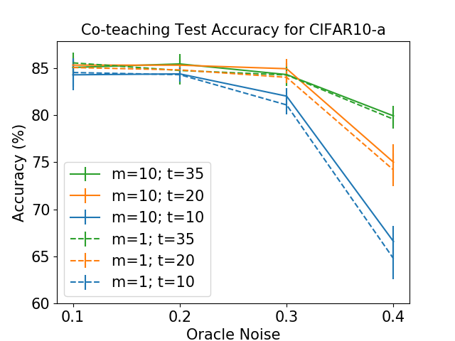
Figure 2 shows the detailed investigation on the Fashion MNIST datasets. It shows similar tendency as the previous Co-teaching results on CIFAR-10 datasets.

5.1.2 Insufficient budget case

In this case, because Algorithm 2 needs to loop over every available hypothesis at each step, it is infeasible to start with a large hypotheses set. Note that even for the MNIST dataset with $784$ features and the simplest linear models, using a discrete exploring space of size $10$ for the parameter corresponding to each feature creates a huge hypotheses set of size $10^{784}$ . Therefore, in order to illustrate the feasibility of the algorithm, we used $2$ -dimensional toy data generated from two Gaussian distributions that are symmetric to the origin point. Specifically, we used two Gaussian distributions with mean value of $(2,2)$ and $(-2,-2)$ and the identical matrix as both covariances. From these distributions, we drew ten thousand data points in total, with each data point having an equal probability to be generated from either distribution. Then a logistic regression classifier is trained with one hundred thousand maximum iteration to simulate the oracles. For the hypothesis set, we used $1000$ equally separated linear classifiers passing through the origin point. Setting the desiring precision $\epsilon=0.1$ resulted three steps based on Algorithm 2. Table 3 shows the number of left candidate hypotheses and their test accuracy at each step.

Table 3: Active Learning Experiment Results

	Step 1	Step 2	Step 3
Number of Left Hypotheses	674.10 (4.97)	525.60 (7.34)	196.90 (71.85)
Test Accuracy of Left Hypotheses	96.98 (0.44)	99.29 (0.19)	99.78 (0.11)

5.2 User study

The previous section investigated the proposed algorithm using artificial oracles, and the feasibility in real-world situations remains untouched. Therefore, we conducted user study using crowdsourcing in this section.

5.2.1 Character recognition task

In this task, we focused on the classification of Kuzushiji (cursive Japanese) [8], which is important for advocating research on Japanese historical books and documents.

Goals

We want to justify the proposed oracle and confirm whether the proposed algorithm can work on results collected through user study without simulation. Specifically, we want to (1) confirm whether data pairs selected by the proposed algorithm are easier for uncertainty comparison than explicit labeling, and (2) confirm whether the proposed algorithm can work on only crowdsourcing results. We will introduce the data and the general interface we used in user study, followed by detailed description of each user study setting in the following paragraphs.

Data

From the Kuzushiji-MNIST dataset [8], we selected the $5$ -th and the $10$ -th characters to form the binary classification task. The reading alphabet is ‘NA’ for the $5$ -th character and ‘WO’ for the $10$ -th character. Figure 3 shows them in a standard font. Albeit the visual similarity, these two characters are important auxiliary words with distinct meanings. Thus, wrongly recognizing the two characters can harm the understanding of the sentence. This recognition task has a natural affinity with uncertainty comparison, as in daily writing, the difficulty of recognizing a hand written character is easier to interpret, rather than recognizing the exact character.

Methods

We prepared three types of questions: explicit labeling, pairwise positivity comparison, and pairwise uncertainty comparison. We also asked annotators for the difficulty of each question when necessary. The interfaces are shown by the following list.

•

Figure 4 shows how we ask annotators for explicit labels.
•

Figure 5 shows how we ask annotators for pairwise positivity comparisons. If we fix one label such as ‘NA’ and ask which one is more likely to be ‘NA’, there are cases that both images in a pair look similar to ‘WO’, thus it’s difficult to answer. Therefore, we also ask annotators to choose either ‘NA’ or ‘WO’ that is used as the criterion of positivity.
•

Figure 6 shows how we ask annotators for pairwise uncertainty comparisons. As this is a newly proposed comparison question and annotators may be not used to answer it, we give an explanatory example on how to select.
•

Figure 7 shows how we ask annotators for difficulty evaluation of uncertainty comparisons compared to explicit labeling. We asked annotators to answer both queries first to familiarize them with the problem.

Justification for uncertainty comparisons

In this user study, we confirmed whether the data pairs selected by the algorithm for $O_{2}$ are difficult for explicit labeling. We first greedily selected $25$ medoids from all data points. Then, we ran the proposed algorithm on these $25$ data points using artificial oracles, and collected the $42$ pairs that were selected for $O_{2}$ . Finally, we conducted user study from $50$ annotators on explicit labeling and uncertainty comparison on these $42$ pairs. For each, we also asked the difficulty of uncertainty comparisons compared to explicit labeling using scores from one to five, with a smaller score indicating an easier question. Furthermore, we collected difficulty evaluation of explicit labeling for each image from $10$ annotators.

In order to investigate the difficulty evaluation on pair attributes, we introduce the individual difficulty for each single image. Another difficulty will be introduced in the following paragraph. Then, based on the user evaluation of individual difficulties, we classified data pairs into three types: (1) the ‘E’ type containing two easy data points, (2) the ‘&’ type containing one easy and one difficult data point, and (3) the ‘D’ type containing two difficult data points.

We then aggregated the user evaluations based on pair types. Table 4 shows the mean and standard deviation of the difficulty evaluations for each type, as well as t statistics and p values when conducted one sample t test against value $3$ , which means two types of query have equal difficulty. From the results, we can conclude that as pair type changes from ‘E’ to ‘D’, uncertainty comparison becomes less favored against explicit labeling. For type ‘D’, the mean of difficulty evaluations is not significantly different from $3$ , as the p value $0.06>0.05$ . However, as the proposed algorithm focuses on separating difficult images, random decisions on images with similar difficulty do not harm the performance.

Table 4: Statistics of difficulty evaluation of uncertainty comparisons.

	Type ‘E’	Type ‘&’	Type ‘D’	Total
Number of Pairs	12	25	5	42
Number of Total Evaluations	600	1250	250	2100
Mean	2.57	2.82	2.84	2.75
Standard Deviation	1.28	1.38	1.35	0.34
t statistic	-8.23	-4.68	-1.91	-5.15
p value	$1.19\times 10^{-15}$	$3.22\times 10^{-6}$	0.06	$4.69\times 10^{-6}$

Algorithm feasibility using simulated pairwise comparisons

In this user study, we first greedily selected $50$ medoids as training data. We then collected explicit label feedback from $20$ annotators. For a single image in these $50$ medoids, we simulated its class probability by the proportion of class assignments in the $20$ evaluations. For example, if $15$ annotators assigned positive label to an image, we defined its probability to be positive as $\frac{15}{20}=0.75$ . These probabilities were then used to simulate both kinds of pairwise comparisons. Using inferred labels as input, the last layer of a pre-trained neural network was fine-tuned.

Figure 8 shows the label accuracy and the test accuracy when using different numbers of medoids as training data. The test accuracy measures the performance of each classifier learnt from inferred labels on a test dataset of size $100$ , which is uniformly selected without replacement excluding the training data points. It can be clearly observed for the full supervision case that more training data contribute higher accuracies. It is not clear for the other two methods, because they rely on not only the number of training data, but also the quality of their pairwise comparison feedback. Although there were $64\%$ ties among all uncertainty pairwise comparisons, the proposed method showed consistent performance. However, with $24\%$ ties among all positivity pairwise comparisons, the existing method failed to perform consistently, even with parameter tuning.

Algorithm feasibility using user feedback on pairwise comparisons

In this user study, we confirmed the performance of each algorithm on only crowdsourcing results. We greedily selected $25$ medoids [26], collected answers for all possible combinations among these medoids from $10$ annotators, and used aggregated majority as input to the existing algorithm [31] using both positivity comparisons and explicit class labels and the proposed algorithm. We adopted a pre-trained neural network and fine-tuned its last layer considering the small number of training data.

Figure 9 and Figure 10 show the label accuracies and test accuracies for results of $25$ greedily selected medoids and $25$ uniformly selected data points, respectively. The test accuracy measures the performance of each classifier learnt from inferred labels on a test dataset of size $100$ , which is uniformly selected without replacement after the selection of training data points. For label accuracies, we calculated the scores for each trial. For test accuracies, we uses aggregated results and calculated only once. The mean value from results of $10$ annotators are shown in dashed lines and the standard deviation are shown by the shadow. The value from aggregated results are shown in solid lines. The proposed algorithm showed competitive performance to fully supervised learning without accessing explicit class labels at all.

When increasing the number of training data, we observed the proposed algorithm could also show stable and promising generalization ability competitive with full supervision. However, the performance of the existing algorithm [31] was not stable, because it separated data points into small bags, and queried a random subset of each bag for explicit class labels. With fewer training data, the size of each bag was small and it could query most of a bag for explicit class labels, thus achieved high labeling accuracy. However, with more training data, a reasonable budget restrained the size of the subset from each bag for querying explicit class labels, thus resulting the drop in performance.

Then we analysed the properties of pairs selected for $O_{2}$ . Different from last paragraph, these pairs were selected by the algorithm ran on crowdsourcing results. We introduce another type of difficulty: pair difficulty for a pair of data points. We investigated the relationship between pair types and pair difficulties. The user evaluation of pair difficulties were $0.16\,(\pm 0.33)$ , $0.17\,(\pm 0.10)$ and $0.56\,(\pm 0.09)$ , respectively. It matches the intuition that annotators confused when both images were difficult to classify.

Figure 11 shows the trajectories of actually queried uncertainty comparisons of $10$ trials, indicating easy pairs by white and difficult pairs by orange. Note that each query consisted of a pair of images. Taking Trial $02$ as an example, we observe that for the first query, an annotator found it easy to assign the explicit class label to one image and difficult for the other. This also holds for the second query. The same annotator then found it difficult to assign explicit class labels to both images in the third query. Another annotator found it easy to compare uncertainties than explicit labeling images in the first and second queries, and difficult for the third query. We can observe that more difficult pairs are queried on the latter half of the executions. This can be interpreted that the algorithm successfully separated difficult data from easy data at an early stage. Note that for the purpose of separating data by different difficulties, the results of ‘E’ pairs and ‘D’ pairs do not effect too much as the data points in these pairs have similar difficulty.

Figure 12 shows the corresponding histogram. As pair type becoming difficult, the proportion of pairs evaluated as difficult for uncertainty comparison increased as expected. Although blue areas are more preferable than orange areas, the proposed algorithm is not significantly influenced by the orange proportion of ‘D’ pairs.

User comments

At the end of each questionnaire, we also asked annotators to answer their opinions on these tasks in free text. We select some of representative opinions and list their English translation ¹¹1The translation is based on the results of DeepL (https://www.deepl.com/translator)..

The following list shows advantages of positivity comparisons over explicit labeling.

•

It is easy to choose between “NA" or “WO" even if you can’t read the word.
•

You can choose the one you can easily recognize.
•

You can choose the letters by your feeling.
•

Unlike direct judgments, there is no clear correct answer, so it is possible to create questions that are easy for anyone to answer.
•

When it’s not too curled up, it’s easy to choose.

The following list shows disadvantages of positivity comparisons over explicit labeling.

•

If you cannot read either of them, your selection criteria will be blurred.
•

It is hard to judge a flaw when it’s curled up.
•

It is not sure if the decision is accurate.
•

You need to stop and compare both images carefully, and may feel a great sense of hesitation before making a decision.
•

Unlike direct judgement, there is no clear correct answer, and if neither letter is difficult to judge, you don’t have to think about the answer. You can make a good choice.

The following list shows advantages of uncertainty comparisons over explicit labeling.

•

It’s easy to choose if you can read one or the other somehow.
•

It’s quick and intuitive and I understand it quickly.
•

Can be narrowed down if both are recognized as “NA" or “WO".
•

It’s easy to imagine how easy it is to read by just the simple criterion of being able to read, and how easy it is to read by pronouncing it in your head.
•

It is highly flexible and does not have any restrictions.

The following list shows disadvantages of uncertainty comparisons over explicit labeling.

•

You can only seem to read them, but you can’t tell whether you actually chose the correct answer or not.
•

I don’t know if other people can quickly recognize.
•

If the words are not read as “NA" or “WO", I use the elimination method to select.
•

When neither of them is likely to be readable, I tend to choose them at random.
•

Unlike direct judgments, there is no clear correct answer, which makes it difficult to evaluate the competence of the annotator.

As we can see from above lists, it is difficult to choose when both images in a pair are not recognizable. This may affect the accuracy of the existing method, as it is required to sort the whole dataset. However, this does not significantly downgrade the performance of the proposed algorithm, as either one in the pair satisfying the desired uncertainty. Moreover, it is interesting to see the various criterion used by annotators.

5.3 Car preference task

The pairwise positivity oracle $O_{1}$ is extensively used in preference learning. Thus in this study, we used a car dataset [17] to simulate a binary classification using user preference, denoting car images a user likes as positive and those a user dislikes as negative. Note the true labels differ for each user, as different users may have different preferences for cars.

Goals

We want to verify if the proposed comparison oracle is useful for binary classification of individual user preference.

Method

In this user study, we conducted crowdsourcing in two ways.

•

First, we collected user preference by five-stage evaluation. Stage one indices the user likes the car very much and stage five indices the opposite. This can be seen as different ranges of $p(y=1|x)$ for a given image $x$ , thus can be used to simulate both pairwise comparison oracles. For eliciting explicit labels, we considered the first two stages as positive.
•

Second, we directly collected user feedback of two kinds of pairwise comparisons on all possible pairs for a fixed set of training data.

We used an interface that is similar to the one used in the first user study.

Data

The original dataset [17] consists of $196$ categories. We trained a ResNet18 [15] model for classifying car categories to extract useful features. Based on extracted features, we greedily selected a single medoid for each class to collect $196$ images. For the first crowdsourcing task on five-stage evaluation, we then uniformly selected $150$ images. For the second task, we greedily selected $25$ medoids based on extracted features for training and used the left $125$ images for testing. We collected user feedback of all possible $300$ pairs for both kinds of pairwise comparisons. All tasks are answered by four users. After inferring labels, we trained both a neural network classifier and a $k$ -NN classifier for each setting.

Algorithm feasibility using simulated pairwise comparisons

Using five-stage evaluation to simulate pairwise comparisons, we had the freedom of choosing various sets of training data points. Thus, we conducted experiments with different sizes of training data points that are selected either uniformly or greedily as medoids using extracted features. The simulated feedback was noisy in the sense that when two images has same stage evaluation, we can only randomly answer one with equal probability.

As shown in Figure 13, the proposed method using only simulated pairwise comparisons showed competitive performance to fully supervision. The performance of the existing method was not stable, because the quick sort subroutine is very sensitive to the results of pairwise comparison, which could be random in this case. However, the proposed algorithm showed consistent performance under the same situation.

User Comments

After a user finished answering all questions, we asked comments on the following open questions. The answers below are summaries of comments from four users.

Question $1$ : What are the characteristics of pairs that are easy for preference uncertainty comparison.

•

When one of the car falls in the middle of like and dislike, or falls in a preferred category.
•

When two cars are completely different from each other.

Question $1$ : What are the characteristics of pairs that are difficult for preference uncertainty comparison.

•

When two cars have similar appearance or preference.

Question $3$ : What factors decide the difficulty of preference uncertainty comparison.

•

Appearance; category; experience.

Question $4$ : What other items that preference uncertainty comparison may work?

•

Food; plants; shoes; cloth; things that are unusual in daily life.

Question $5$ : What other measures other than preference uncertainty comparison may work?

•

Fairness; measures that everyone is familiar with; measures that based on experience.

6 Conclusion

In this paper, we address the problem of interactive labeling and propose a novel uncertainty comparison oracle, followed by a noise-tolerant theoretical-guaranteed labeling algorithm without accessing explicit class labels at all. We then confirm the performance of the algorithm theoretically and empirically. For future work, eliminating $\mathcal{O}(n)$ from one of the query complexity can improve the efficiency. On the other hand, extending the uncertainty comparison oracle to multiple data points and multiple classes is a promising direction.

Broader Impact

We believe this research will benefit researchers in all fields who are seeking for a more effective and less laborious annotation method for their unlabeled datasets. It can foster applications of machine learning by lowering the annotation barrier for people without specific professional knowledge. It can also benefit domain experts with professional knowledge by saving their time for more important tasks. Furthermore, collecting comparison information can potentially mitigate annotation biases of explicit labeling. It can also serve the aim of protecting privacy by not querying the explicit class labels in some cases.

For the negative side, it may harm the performance of downstream classification models when the comparison annotation is mostly incorrect. However, there would be no consequential ethical issues of failure of the method.

References

[1] Naomi S Altman. An introduction to kernel and nearest-neighbor nonparametric regression. The American Statistician, 46(3):175–185, 1992.
[2] Maria Florina Balcan and Steve Hanneke. Robust interactive learning. In Conference on Learning Theory, pages 20–1, 2012.
[3] Han Bao, Gang Niu, and Masashi Sugiyama. Classification from pairwise similarity and unlabeled data. In International Conference on Machine Learning, pages 452–461, 2018.
[4] Alina Beygelzimer, Daniel J Hsu, John Langford, and Chicheng Zhang. Search improves label for active learning. In Advances in Neural Information Processing Systems, pages 3342–3350, 2016.
[5] Ralph Allan Bradley and Milton E Terry. Rank analysis of incomplete block designs: I. the method of paired comparisons. Biometrika, 39(3/4):324–345, 1952.
[6] Kamalika Chaudhuri and Sanjoy Dasgupta. Rates of convergence for nearest neighbor classification. In Advances in Neural Information Processing Systems, pages 3437–3445, 2014.
[7] Wei Chu and Zoubin Ghahramani. Preference learning with gaussian processes. In Proceedings of the 22nd International Conference on Machine Learning, ICML ’05, page 137–144, New York, NY, USA, 2005. Association for Computing Machinery.
[8] Tarin Clanuwat, Mikel Bober-Irizar, Asanobu Kitamoto, Alex Lamb, Kazuaki Yamamoto, and David Ha. Deep learning for classical japanese literature. preprint, 2018.
[9] Zhenghang Cui, Nontawat Charoenphakdee, Issei Sato, and Masashi Sugiyama. Classification from triplet comparison data. Neural Computation, 32(3):659–681, 2020.
[10] Marthinus Christoffel Du Plessis, Gang Niu, and Masashi Sugiyama. Clustering unclustered data: Unsupervised binary labeling of two datasets having different class balances. In 2013 Conference on Technologies and Applications of Artificial Intelligence, pages 1–6. IEEE, 2013.
[11] Johannes Fürnkranz and Eyke Hüllermeier. Preference learning and ranking by pairwise comparison. In Preference learning, pages 65–82. Springer, 2010.
[12] Wei Gao, Bin-Bin Yang, and Zhi-Hua Zhou. On the resistance of nearest neighbor to random noisy labels. arXiv preprint arXiv:1607.07526, 2016.
[13] Bo Han, Quanming Yao, Xingrui Yu, Gang Niu, Miao Xu, Weihua Hu, Ivor Tsang, and Masashi Sugiyama. Co-teaching: Robust training of deep neural networks with extremely noisy labels. In NeurIPS, pages 8535–8545, 2018.
[14] Steve Hanneke et al. Theory of disagreement-based active learning. Foundations and Trends® in Machine Learning, 7(2-3):131–309, 2014.
[15] Kaiming He, Xiangyu Zhang, Shaoqing Ren, and Jian Sun. Deep residual learning for image recognition. In Proceedings of the IEEE conference on computer vision and pattern recognition, pages 770–778, 2016.
[16] Daniel M Kane, Shachar Lovett, Shay Moran, and Jiapeng Zhang. Active classification with comparison queries. In 2017 IEEE 58th Annual Symposium on Foundations of Computer Science (FOCS), pages 355–366. IEEE, 2017.
[17] Jonathan Krause, Michael Stark, Jia Deng, and Li Fei-Fei. 3d object representations for fine-grained categorization. In 4th International IEEE Workshop on 3D Representation and Recognition (3dRR-13), Sydney, Australia, 2013.
[18] Alex Krizhevsky, Geoffrey Hinton, et al. Learning multiple layers of features from tiny images. preprint, 2009.
[19] Yann LeCun, Léon Bottou, Yoshua Bengio, and Patrick Haffner. Gradient-based learning applied to document recognition. Proceedings of the IEEE, 86(11):2278–2324, 1998.
[20] Nan Lu, Gang Niu, Aditya K. Menon, and Masashi Sugiyama. On the minimal supervision for training any binary classifier from only unlabeled data. In International Conference on Learning Representations, 2019.
[21] R Duncan Luce. Individual choice behavior: A theoretical analysis. Courier Corporation, 2012.
[22] Enno Mammen, Alexandre B Tsybakov, et al. Smooth discrimination analysis. The Annals of Statistics, 27(6):1808–1829, 1999.
[23] Soheil Mohajer, Changho Suh, and Adel Elmahdy. Active learning for top- $k$ rank aggregation from noisy comparisons. In Doina Precup and Yee Whye Teh, editors, Proceedings of the 34th International Conference on Machine Learning, volume 70 of Proceedings of Machine Learning Research, pages 2488–2497. PMLR, 06–11 Aug 2017.
[24] Harikrishna Narasimhan and Shivani Agarwal. On the relationship between binary classification, bipartite ranking, and binary class probability estimation. In Advances in Neural Information Processing Systems, pages 2913–2921, 2013.
[25] Henry Reeve and Ata Kaban. Fast rates for a kNN classifier robust to unknown asymmetric label noise. In Kamalika Chaudhuri and Ruslan Salakhutdinov, editors, Proceedings of the 36th International Conference on Machine Learning, volume 97 of Proceedings of Machine Learning Research, pages 5401–5409, Long Beach, California, USA, 09–15 Jun 2019. PMLR.
[26] Erich Schubert and Peter J Rousseeuw. Faster k-medoids clustering: improving the pam, clara, and clarans algorithms. In International Conference on Similarity Search and Applications, pages 171–187. Springer, 2019.
[27] Takuya Shimada, Han Bao, Issei Sato, and Masashi Sugiyama. Classification from pairwise similarities/dissimilarities and unlabeled data via empirical risk minimization. arXiv preprint arXiv:1904.11717, 2019.
[28] Christopher Tosh and Sanjoy Dasgupta. Interactive structure learning with structural query-by-committee. In Advances in Neural Information Processing Systems, pages 1121–1131, 2018.
[29] Vladimir Vapnik. Statistical learning theory. New York, 3, 1998.
[30] Han Xiao, Kashif Rasul, and Roland Vollgraf. Fashion-mnist: a novel image dataset for benchmarking machine learning algorithms. preprint, 2017.
[31] Yichong Xu, Hongyang Zhang, Kyle Miller, Aarti Singh, and Artur Dubrawski. Noise-tolerant interactive learning using pairwise comparisons. In Advances in Neural Information Processing Systems, pages 2431–2440, 2017.

Appendix A Proof of Theorem 2

Proof.

The Algorithm 1 consists of two steps: selection of relatively uncertain points and assigning labels by majority vote.

For the first step, the algorithm of Mohajer et al. [23] is executed using parameters $K=t$ and $m$ . By adapting Theorem 1 of Mohajer et al. [23], we know that if $m\geq\frac{C_{1}\max(\log\log{n},\log{t})}{(0.5-\epsilon_{2})^{2}}$ , then the correct top- $t$ points can be identified with probability at least $1-{\log{n}}^{-C_{2}}$ .

For the second step, we analyze the probability that a point $x\in D\setminus D^{\prime}$ is correctly inferred. Without loss of generality, we assume the correct label for $x$ is $1$ and we calculate the probability that $\sum_{x_{j}\in D^{\prime}}O_{1}(x,x_{j})\geq\frac{1}{2}$ .

Let $Z_{j}\triangleq O_{1}(x,x_{j})$ denotes the random variable representing the outcome of every call to oracle $O_{1}$ . Because $D^{\prime}$ is assumed to be correctly identified, so $p(y|x)\geq p(y|x_{j})$ for every $x_{j}\in D^{\prime}$ , thus the expectation of $Z_{j}$ is $1-\epsilon_{1}$ . Also note that $Z_{j}$ only takes a value of either $0$ or $1$ , thus by applying Hoeffding’s inequality to $Z_{1},Z_{2},\cdots,Z_{t}$ , we have

\mathrm{Pr}\left[\frac{1}{t}\sum_{j=1}^{t}Z_{j}-(1-\epsilon_{1})\leq-(0.5-\epsilon_{1})\right]\leq\exp\left(-2t(0.5-\epsilon_{1})^{2}\right).

(1)

This actually expresses the probability that $\frac{1}{t}\sum_{j=1}^{t}Z_{j}$ is smaller than $0.5$ .

Let $a\triangleq\exp\left(-2t(0.5-\epsilon_{1})^{2}\right)$ . Because $t$ is selected so that $a\leq\frac{1}{2}$ and $\frac{1}{t}\sum_{j=1}^{t}Z_{j}$ is bounded within $[0,1]$ , therefore for a single $x\in D\setminus D^{\prime}$ it holds that

	$\displaystyle\mathrm{Pr}\left[\frac{1}{t}\sum_{j=1}^{t}Z_{j}\geq\frac{1}{2}\right]$	$\displaystyle\geq 1-a$		(2)
		$\displaystyle\geq\exp(-a(a+1)).$		(3)

For points in $D^{\prime}$ , because we assign random labels, there is positive probability that all assigned labels are wrong.

In conclusion, for all points in $D\setminus D^{\prime}$ correctly labeled, the error rate $\epsilon=\frac{t}{n}$ can be achieved with probability at least $1-\delta$ where $\delta\triangleq 1-(1-\log{n}^{-C_{2}})\exp(-a(a+1)(n-t))$ .

For query complexities, as $O_{1}$ is queried $t(n-t)$ times, the query complexity of $O_{1}$ is $\mathcal{O}\left(\frac{n}{\epsilon_{1}^{2}}\right)$ . Moreover, as indicated by Eq. (17) of [23], the query complexity of $O_{2}$ is $\mathcal{O}\left(\frac{n\log\log{n}}{\epsilon_{2}^{2}}\right)$ . ∎

Appendix B Proof of Theorem 3

Proof.

First, we bound the difference between $\hat{f}(x;k)$ and $f(x)$ . Similar to Reeve et al. [25], we define $\tilde{f}(x;k)=\mathbb{E}_{p(y|x)}=\frac{1}{k}\sum_{q=1}^{k}y_{\tau_{q}(x)}$ .

Then we have

\left|\hat{f}(x;k)-f(x)\right|\leq\left|\hat{f}(x;k)-\tilde{f}(x;k)\right|+\left|\tilde{f}(x;k)-f(x)\right|.

(4)

For the first term in RHS, from Theorem 2, we know it is bounded by $\frac{2\epsilon}{k}$ with probability at least $1-\delta$ . For the second term in right hand side, from Lemma 4.1 in [25], we have it is bounded by $\omega\left(\frac{2k}{n}\right)^{\lambda}$ with probability at least $1-\delta^{\prime}$ for $\delta^{\prime}>0$ and $\frac{n}{2}\geq k\geq 4\log(\frac{1}{\delta^{\prime}})+1$ . Thus combing the two inequalities, we have the left hand side is bounded by $\Delta\triangleq\frac{2\epsilon}{k}+\omega\left(\frac{2k}{n}\right)^{\lambda}$ with probability at least $(1-\delta)(1-\delta^{\prime})$ . This means with at least the same probability, a randomly drawn point from $\mathcal{X}$ will fall in the set

\mathcal{X}^{\prime}\triangleq\{x\in\mathcal{X}:|\hat{\eta}(x)-\eta(x)|\leq\Delta\}.

Thus

		$\displaystyle R(\hat{f})-R(f^{*})$
	$\displaystyle=$	$\displaystyle\int_{\mathcal{X}}\left\|\eta(x)-\frac{1}{2}\right\|\mathbbm{1}_{\hat{f}(x)\neq f^{*}(x)}d\mu(x)$
	$\displaystyle=$	$\displaystyle\int_{\mathcal{X}^{\prime}}\left\|\eta(x)-\frac{1}{2}\right\|\mathbbm{1}_{\hat{f}(x)\neq f^{*}(x)}d\mu(x)\left(\text{with probability at least}(1-\delta)(1-\delta^{\prime})\right)$
	$\displaystyle\leq$	$\displaystyle\int_{\mathcal{X}}\left\|\eta(x)-\frac{1}{2}\right\|\mathbbm{1}_{\left\|\eta(x)-\frac{1}{2}\right\|\leq\Delta}d\mu(x)$
	$\displaystyle\leq$	$\displaystyle C\Delta^{\alpha+1}.$

∎

Appendix C Proof of Corollary 4

Proof.

Similar to the approach in Xu et al. [31], we use induction to show that at the end of every step $i$ , $\mathbb{E}_{\mathcal{P}_{\mathcal{X}}}[h(x)\neq h^{*}(x)]\leq 4\epsilon_{i}$ always holds with probability at least $(1-\delta)^{\log(\frac{1}{\epsilon})}$ for a universal $\delta$ , which is obvious for $i=0$ .

Then, with a little abusing of notations, we have

	$\displaystyle\|{x\in S_{i}:h(x)\neq h^{*}(x)}\|$	$\displaystyle=\|{x\in D_{i}:h(x)\neq h^{*}(x)}\|$
		$\displaystyle\leq\|{x\in D_{i}:h(x)\neq\hat{y}}\|+\|{x\in D_{i}:h^{*}(x)\neq\hat{y}}\|$
		$\displaystyle=2\epsilon_{i}\|S_{i}\|.$

Thus $\text{P}_{x\sim S_{i}}[h(x)\neq h^{*}(x)]=\frac{|{x\in S_{i}:h(x)\neq h^{*}(x)}|}{|S_{i}|}\leq 2\epsilon_{i}$ . Having $c_{0}\in(1,\infty)$ and $\gamma\in(0,1)$ , using Lemma 3.1 from Hanneke et al. [14], we have $\text{P}_{x\sim\mathcal{P}_{\mathcal{X}}}[h(x)\neq h^{*}(x)]\leq 4\epsilon_{i}$ with probability at least $1-\gamma$ , providing $c_{0}\frac{d\log(\frac{|S_{i}|}{d})+\log(\frac{1}{\gamma})}{|S_{i}|}\leq\epsilon_{i}$ . Setting $\gamma=1-(1-\delta)^{\log(2\epsilon)}$ , We have $\text{P}_{\mathcal{P}_{\mathcal{X}}}[\hat{h}(x)\neq h^{*}(x)]\leq\epsilon$ with probability at least $(1-\delta)^{\log(\frac{1}{\epsilon})}(1-\delta)^{\log(2\epsilon)}=1-\delta$ at the end of the algorithm. ∎

	$\displaystyle\|{x\in S_{i}:h(x)\neq h^{*}(x)}\|$	$\displaystyle=\|{x\in D_{i}:h(x)\neq h^{*}(x)}\|$
		$\displaystyle\leq\|{x\in D_{i}:h(x)\neq\hat{y}}\|+\|{x\in D_{i}:h^{*}(x)\neq\hat{y}}\|$
		$\displaystyle=2\epsilon_{i}\|S_{i}\|.$

Active Classification with Uncertainty Comparison Queries

Abstract

1 Introduction

2 Labeling with pairwise comparisons

2.1 Preliminaries

2.2 Two pairwise comparison oracles

Positivity comparison oracle

Condition 1.

Uncertainty comparison oracle

Condition 2.

2.3 Proposed labeling algorithm

Top selection algorithm from noisy comparisons [23]

Theorem 1 (Mohajer et al. [23]).

2.4 Learning classifiers under different budgets

Sufficient budget case

Insufficient budget case

3 Theoretical analysis

3.1 Analysis of the proposed labeling algorithm

Theorem 2 (Error rate bound).

3.2 Analysis of nearest neighbors classifiers

Assumption 1 (Measure smoothness [6]).

Assumption 2 (Tsybakov’s margin condition).

Theorem 3 (Generalization error bound for kk-NN).

3.3 Analysis of disagreement-based active learning

Corollary 4 (Generalization error bound for active learning).

4 Related work

Weakly-supervised learning

Preference learning

Active learning

5 Experiments

5.1 Simulation study

5.1.1 Sufficient budget case

5.1.2 Insufficient budget case

5.2 User study

5.2.1 Character recognition task

Goals

Data

Methods

Justification for uncertainty comparisons

Algorithm feasibility using simulated pairwise comparisons

Algorithm feasibility using user feedback on pairwise comparisons

User comments

5.3 Car preference task

Goals

Method

Data

Algorithm feasibility using simulated pairwise comparisons

User Comments

6 Conclusion

Broader Impact

References

Appendix A Proof of Theorem 2

Proof.

Appendix B Proof of Theorem 3

Proof.

Appendix C Proof of Corollary 4

Proof.

Theorem 3 (Generalization error bound for $k$ -NN).