ACPO: A Policy Optimization Algorithm for Average MDPs with Constraints
Abstract
Reinforcement Learning (RL) for constrained MDPs (CMDPs) is an increasingly important problem for various applications. Often, the average criterion is more suitable than the discounted criterion. Yet, RL for average-CMDPs (ACMDPs) remains a challenging problem. Algorithms designed for discounted constrained RL problems often do not perform well for the average CMDP setting. In this paper, we introduce a new policy optimization with function approximation algorithm for constrained MDPs with the average criterion. The Average-Constrained Policy Optimization (ACPO) algorithm is inspired by trust region-based policy optimization algorithms. We develop basic sensitivity theory for average CMDPs, and then use the corresponding bounds in the design of the algorithm. We provide theoretical guarantees on its performance, and through extensive experimental work in various challenging OpenAI Gym environments, show its superior empirical performance when compared to other state-of-the-art algorithms adapted for the ACMDPs.
1 Introduction
Over the last decade, we have seen an enormous impact of RL techniques on a variety of problems, from mastering complex games like Go (Silver et al., 2017) and StarCraft (Vinyals et al., 2019) to robotic control (Levine et al., 2016; Akkaya et al., 2019; Aractingi et al., 2023). Many of these have used RL-policy optimization algorithms such as Schulman et al. (2017) for discounted MDPs (DMDPs). These have come in handy even in generative AI, e.g., training large language models (LLMs) (Achiam et al., 2023). However, applications often need satisfaction of some constraints, e.g., physical safety of mobile robots (Hu et al., 2022), safe language, image or multi-modal output generation. Furthermore, the average criterion when long-term rewards and safety are of consideration is more suitable. Using discounted cost formulations (as a proxy for safety) incentivizes policy optimization algorithms to search for policies that are short-term safe but not long-term because of future-discounting.
The planning problem for MDPs with constraints is often formulated as a Constrained MDP (CMDP) model (Manne, 1960; Hordijk & Kallenberg, 1979; Altman, 1999). Unfortunately, CMDP models do not satisfy Bellman’s principle of optimality, and hence dynamic programming (DP)-style algorithms cannot be developed for the setting. Instead, an alternative approach called the convex analytic approach (Borkar, 1988; Altman, 1999) is used by way of introducing occupation measures that leads to optimization formulations. This can be done for both discounted (DCMDPs) and average-criterion (ACMDPs) constrained MDPs.
Theory and algorithms for RL deal with settings when the MDP model is unknown. While DP-inspired RL algorithms such as DQN, when combined with deep learning architectures for function approximation work remarkably effectively (Mnih et al., 2015), policy optimization algorithms such as TRPO (Schulman et al., 2015), PPO (Schulman et al., 2017) have proven even more effective in solving high dimensional problems. Since the discounted criterion is sometimes not suitable, policy optimization algorithms such as ATRPO (Zhang et al., 2021; Wan et al., 2021; Liao et al., 2022) have been developed for AMDPs. Furthermore, as already mentioned, certain RL applications have multiple objectives, one of which is to be optimized and the rest constrained. Thus, the Constrained Policy Optimization (CPO) algorithm (Achiam et al., 2017) was introduced for infinite-horizon DCMDP problems. Unfortunately, as motivated above, not all such applications fit the discounted-criterion formulation: there are settings, for example where there may be safety requirements when the average-CMDP model is a better fit. No scalable RL algorithms are currently available for such settings.
We note that the RL problem is usually harder than the corresponding planning problem; average-MDPs are more challenging than discounted MDPs; and constrained MDPs are more challenging than unconstrained ones. In this paper, we present the first practical algorithm for policy optimization-based RL algorithm for average-constrained MDPs. We propose ACPO, a policy optimization algorithm for an average-CMDP with deep learning for function approximation. Our approach is motivated by theoretical guarantees that bound the difference between the average long-run rewards or costs of different policies. It draws inspiration from CPO (Achiam et al., 2017) (see also Tessler et al. (2019) for DCMDPs), which uses a policy improvement theorem for the discounted setting based on the trust region methods of Schulman et al. (2015). Unfortunately, this result trivializes for the average setting and hence can’t be used. Instead, we derive a new bound that depends on the worst-case level of “mixture” of the irreducible Markov chain associated with a policy. Our proposed algorithm, ACPO is based on these theoretical developments. For experimental evaluation, we use several OpenAI Gym environments from Todorov et al. (2012), train large neural network policies and demonstrate the effectiveness and superior performance of the ACPO algorithm as compared to others.
Main Contributions and Novelty.
Algorithmic: We introduce the first practical policy optimization-based RL algorithm for average-constrained MDPs with new and tight performance bounds and violation guarantees. The algorithm draws inspiration from CPO (for discounted-CMDPs) and ATRPO (for average-MDPs) but is not a straightforward extension of either. One may posit that setting the discount factor in CPO for the discounted setting may suffice but that does not perform well on average-CMDPs even with a large discount factor. Further, constraint violation and policy degradation bounds of CPO do not hold in the average setting and hence we develop novel bounds (in Corollary 3.5). In fact, the advantage function estimation routine in our algorithm (line 4 and 6 in Algorithm 1) is also different from that in CPO, since the discounted-setting procedure cannot be used for the average setting (see Appendix A.3): We first approximate the average-reward bias and then use a one-step TD backup to estimate the action-bias function. Furthermore, policy optimization algorithms for the average case (Zhang & Ross, 2020; Wan et al., 2021; Liao et al., 2022) cannot incorporate constraints. We enable this by introducing sublevel sets of cost constraints. We also introduce an approximate but novel line search procedure that improves the empirical performance of our algorithm, an idea that may help improve performance of other policy optimization algorithms such as PPO.
Technical: Since ACPO is a trust region method, one can expect some overlap in analysis techniques with other similar algorithms. Nevertheless, our analysis has several novel elements: Lemma 3.3, where we use eigenvalues of the transition matrix to relate total variation of stationary distributions with that of the policies, and in Lemma A.3, we use the sublevel sets of constraints and projection inequality of Bregman divergence. Furthermore, several important results from CPO and ATRPO papers cannot be applied to the analysis of our algorithm.
Empirical: We evaluate the empirical performance of ACPO in the OpenAI Gym (Mujoco) environments, a standard benchmark. We find that ACPO outperforms all state-of-the-art Deep RL algorithms such as CPO in (Achiam et al., 2017), PCPO in (Yang et al., 2020), PPO in (Schulman et al., 2017), BVF-PPO in (Satija et al., 2020) and ATRPO in (Zhang et al., 2021). We use a large discount factor if the algorithm is not for the average setting, and a Lagrangian objective if it is not for the constrained setting, and in some cases both.
Significance: ACPO is the first practical trust region-style policy optimization algorithm for ACMDPs with excellent empirical performance. ACMDPs are important models because they allow incorporation of long term safety constraints, which are important not only in the context of safe robot learning and control, but also safety-constrained RLHF fine-tuning and inference for LLMs (Moskovitz et al., 2023) and Diffusion models as well. In the absence of suitable policy optimization algorithms for ACMDPs, researchers have resorted to using adaptations of PPO, etc.
Related Work. Learning constraint-satisfaction policies has been explored in the Deep RL literature in (Agnihotri et al., 2019; Garcia & Fernandez, 2015). This can either be (1) through expert annotations and demonstrations as in (Rajeswaran et al., 2017; Gao et al., 2018) or, (2) by exploration with constraint satisfaction as in (Achiam et al., 2017; Tessler et al., 2019). While the former approach is not scalable since it requires human interventions, current state-of-the-art algorithms for the latter are not applicable to the average reward setting.
Previous work on RL with the average reward criterion has mostly attempted to extend stochastic approximation schemes for the tabular setting, such as Q-learning in (Abounadi et al., 2001; Wan et al., 2021), to the non-tabular setting with function approximation in (Wei et al., 2021; Zhang & Ross, 2020). (Chen et al., 2022) deals with online learning in a constrained MDP setting, but their aim is regret minimization or exploration, both in tabular settings. We are inspired by the work of (Zhang et al., 2021) to develop techniques required to derive the policy degradation and constraint violation bounds in Section 3.
The more recent works of (Bhatnagar & Lakshmanan, 2012) and (Calvo-Fullana et al., 2023) also fail to address our problem setting as the former test on a 2x4 queueing network with maximum state space of 128, while the latter test on a grid of size 10x10 (maximum states of 100). In addition to that, the way they incorporate constraints during training is just via a Lagrangian formulation. In our paper we show that simply doing this (in the case of PPO and ATRPO for example) leads to much inferior performance to ACPO, which can outperform current state-of-the-art algorithms in state spaces of upto .
2 Preliminaries
A Markov decision process (MDP) is a tuple, (), where is the set of states, is the set of actions, is the reward function, is the transition probability function such that is the probability of transitioning to state from state by taking action , and is the initial state distribution. A stationary policy is a mapping from states to probability distributions over the actions, with denoting the probability of selecting action in state , and is the probability simplex over the action space . We denote the set of all stationary policies by . For the average setting, we will make the standard assumption that the MDP is ergodic and is unichain.
In reinforcement learning, we aim to select a policy which maximizes a performance measure, , which, for continuous control tasks is either the discounted reward criterion or the average reward approach. Below, we briefly discuss both formulations.
2.1 Discounted criterion
For a given discount factor , the discounted reward objective is defined as
|
|
where refers to a sample trajectory of generated when following a policy , that is, and ; is the discounted occupation measure that is defined by , which essentially refers to the discounted fraction of time spent in state while following policy .
2.2 Average criterion
The average-reward objective is given by:
| (1) |
where is the stationary state distribution under policy . The limits in and are guaranteed to exist under our ergodic assumption. Since the MDP is aperiodic, it can also be shown that . Since we have , it can be shown that .
In the average setting, we seek to keep the estimate of the state value function unbiased and hence, introduce the average-reward bias function as
and the average-reward action-bias function as
Finally, define the average-reward advantage function as .
2.3 Constrained MDPs
A constrained Markov decision process (CMDP) is an MDP augmented with constraints that restrict the set of allowable policies for that MDP. Specifically, we augment the MDP with a set of auxiliary cost functions, (with each function mapping transition tuples to costs, just like the reward function), and bounds . Similar to the value functions being defined for the average reward criterion, we define the average cost objective with respect to the cost function as
| (2) |
where will be referred to as the average cost for constraint . The set of feasible stationary policies for a CMDP then is given by . The goal is to find a policy such that
However, finding an exact is infeasible for large-scale problems. Instead, we aim to derive an iterative policy improvement algorithm that given a current policy, improves upon it by approximately maximizing the increase in the reward, while not violating the constraints by too much and not being too different from the current policy.
Lastly, analogous to , , and , we define similar quantities for the cost functions , and denote them by , , and .
2.4 Policy Improvement for discounted CMDPs
In many on-policy constrained RL problems, we improve policies iteratively by maximizing a predefined function within a local region of the current best policy as in (Tessler et al., 2019; Achiam et al., 2017; Yang et al., 2020; Song et al., 2020). (Achiam et al., 2017) derived a policy improvement bound for the discounted CMDP setting as:
| (3) | ||||
where is the discounted version of the advantage function, , and is the total variational divergence between and at . These results laid the foundations for on-policy constrained RL algorithms as in(Wu et al., 2017; Vuong et al., 2019).
However, Equation (3) does not generalize to the average setting () (see Appendix A.1). In the next section, we will derive a policy improvement bound for the average case and present an algorithm based on trust region methods, which will generate almost-monotonically improving iterative policies. Proofs of theorems and lemmas, if not already given, are available in Appendix A.
3 ACPO: The Average-Constrained Policy Optimization Algorithm
In this section, we present the main results of our work. For conciseness, we denote by the column vector whose components are and to be the state transition probability matrix under policy .
3.1 Policy Improvement for the Average-CMDP
Let be the policy obtained via some update rule from the current policy . Analogous to the discounted setting of a CMDP, we would like to characterize the performance difference by an expression which depends on and some divergence metric between the two policies.
Lemma 3.1.
(Zhang & Ross, 2020) Under the unichain assumption of the underlying Markov chain, for any stochastic policies and :
| (4) |
Note that this difference depends on the stationary state distribution obtained from the new policy, . This is computationally impractical as we do not have access to this . Fortunately, by use of the following lemma we can show that if and are “close” with respect to some metric, we can approximate Eq. (4) using samples from .
Lemma 3.2.
Under the unichain assumption, for any stochastic policies and we have:
| (5) |
, where . See Appendix A.1 for proof. Lemma 3.2 implies when and are “close”. Now that we have established this approximation, we need to study the relation of how the actual change in policies affects their corresponding stationary state distributions. For this, we turn to standard analysis of the underlying Markov chain of the CMDP.
Under the ergodic assumption, we have that is irreducible and hence its eigenvalues are such that and . For our analysis, we define , and from (Levene & Loizou, 2002) and (Doyle, 2009), we connect to the sensitivity of the stationary distributions to changes in the policy using the result below.
Lemma 3.3.
Under the ergodic assumption, the divergence between the stationary distributions and is upper bounded as:
| (6) |
, where . See Appendix A.1 for proof. This bound is tighter and easier to compute than the one given by (Zhang et al., 2021), which replaces by , where is known as Kemeny’s constant from (Kemeny & Snell, 1960). It is interpreted as the expected number of steps to get to any goal state, where the expectation is taken with respect to the stationary-distribution of those states.
Proposition 3.4.
Under the ergodic assumption, the following bounds hold for any stochastic policies and :
| (7) |
where
It is interesting to compare the inequalities of Equation (7) to Equation (4). The term in Prop. 3.4 is somewhat of a surrogate approximation to , in the sense that it uses instead of . As discussed before, we do not have access to since the trajectories of the new policy are not available unless the policy itself is updated. This surrogate is a first order approximation to in the parameters of in a neighborhood around as in (Kakade & Langford, 2002). Hence, Eq. (7) can be viewed as bounding the worst-case approximation error.
Extending this discussion to the cost function of our CMDP, similar expressions follow immediately.
Corollary 3.5.
For any policies , and any cost function , the following bound holds:
| (8) |
where
Until now, we have been dealing with bounds given with regards to the TV divergence of the policies. However, in practice, bounds with respect to the KL divergence of policies is more commonly used as in (Schulman et al., 2015, 2016; Ma et al., 2021). From Pinsker’s and Jensen’s inequalities, we have that
| (9) |
We can thus use Eq. (9) in the bounds of Proposition 3.4 and Corollary 3.5 to make policy improvement guarantees, i.e., if we find updates such that , then we will have monotonically increasing policies as, at iteration , , for , implying that . However, this sequence does not guarantee constraint satisfaction at each iteration, so we now turn to trust region methods to incorporate constraints, do policy improvement and provide safety guarantees.
3.2 Trust Region Based Approach
For large or continuous state and action CMDPs, solving for the exact optimal policy is impractical. However, trust region-based policy optimization algorithms have proven to be effective for solving such problems as in (Schulman et al., 2015, 2016, 2017; Achiam, 2017). For these approaches, we usually consider some parameterized policy class for tractibility. In addition, for CMDPs, we also require the policy iterates to be feasible, so instead of optimizing just over , we optimize over . However, it is much easier to solve the above problem if we introduce hard constraints, rather than limiting the set to . Therefore, we now introduce the ACPO algorithm, which is inspired by the trust region formulations above as the following optimization problem:
| (10) | ||||
| s.t. | ||||
where , is the average advantage function defined earlier, and is a step size. We use this form of updates as it is an approximation to the lower bound given in Proposition 3.4 and the upper bound given in Corollary 3.5.
In most cases, the trust region threshold for formulations like Eq. (10) are heuristically motivated. We now show that it is quantitatively motivated and comes with a worst case performance degradation and constraint violation. Proof is in Appendix A.2.
Theorem 3.6.
Remark 3.7. Note that if the constraints are ignored (by setting ), then this bound is tighter than given in (Zhang et al., 2021) for the unconstrained average-reward setting.
However, the update rule of Eq. (10) is difficult to implement in practice as it takes steps that are too small, which degrades convergence. In addition, it requires the exact knowledge of which is computationally infeasible for large-scale problems. In the next section, we will introduce a specific sampling-based practical algorithm to alleviate these concerns.
4 Practical Implementation of ACPO
In this section, we introduce a practical version of the ACPO algorithm with a principle recovery method. With a small step size , we can approximate the reward function and constraints with a first order expansion, and approximate the KL divergence constraint with a second order expansion. This gives us a new optimization problem which can be solved exactly using Lagrangian duality.
4.1 An Implementation of ACPO
Since we are working with a parameterized class, we shall now overload notation to use as the policy at iteration , i.e., . In addition, we use to denote the gradient of the advantage function objective, to denote the gradient of the advantage function of the cost , as the Hessian of the KL-divergence. Formally,
In addition, let . The approximation to the problem in Eq. (10) is:
| (13) | ||||
| s.t. | ||||
| and, |
This is a convex optimization problem in which strong duality holds, and hence it can be solved using a Lagrangian method. The update rule for the dual problem then takes the form
| (14) |
where and are the Lagrange multipliers satisfying the dual
| (15) |
with , , , and .
4.2 Feasibility and Recovery
The approximation regime described in Eq. (13) requires to be invertible. For large parametric policies, is computed using the conjugate gradient method as in (Schulman et al., 2015). However, in practice, using this approximation along with the associated statistical sampling errors, there might be potential violations of the approximate constraints leading to infeasible policies.
To rectify this, for the case where we only have one constraint, one can recover a feasible policy by applying a recovery step inspired by the TRPO update on the cost surrogate as:
|
|
(16) |
where . Contrasting with the policy recovery update of (Achiam et al., 2017) which only uses the cost advantage function gradient , we introduce the reward advantage function gradient as well. This choice is to ensure recovery while simultaneously balancing the “regret” of not choosing the best (in terms of the objective value) policy . In other words, we wish to find a policy as close to in terms of their objective function values. We follow up this step with a simple linesearch to find feasible . Based on this, Algorithm 1 provides a basic outline of ACPO. For more details of the algorithm, see Appendix A.3.
Average Rewards:


 Average Constraint values:
5 Empirical Results
We conducted a series of experiments to evaluate the relative performance of the ACPO algorithm and answer the following questions: (i) Does ACPO learn a sequence of constraint satisfying policies while maximizing the average reward in the long run? (ii) How does ACPO compare with the already existing constraint policy optimization algorithms which are applied with a large discount factor? (iii) What are the factors that affect the performance of ACPO?
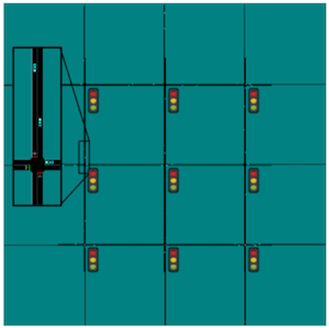
We work with the OpenAI Gym environments to train the various learning agent on the following tasks - Gather, Circle, Grid, and Bottleneck tasks (see Figure 3 in Appendix A.6.1 for more details on the environments). For our experiments we only work with a single constraint with policy recovery using Eq. (16) (this is only a computational limitation; ACPO in principle can handle multiple constraints). We compare ACPO with the following baseline algorithms: CPO by (Achiam et al., 2017), ATRPO by (Zhang et al., 2021), PCPO by (Yang et al., 2020) (a close variant of CPO), BVF-PPO by (Satija et al., 2020) and PPO by (Schulman et al., 2017).
Although ATRPO and PPO originally do not incorporate constraints, for fair comparison, we introduce constraints using a Lagrangian. Also, CPO, PCPO and PPO are compared with . See Appendix A.5 for more details.
5.1 Evaluation Details and Protocol
For the Gather and Circle tasks we test two distinct agents: a point-mass (), and an ant robot (). The agent in the Bottleneck task in , and for the Grid task is . We use two hidden layer neural networks to represent Gaussian policies for the tasks. For Gather and Circle, size is (64,32) for both layers, and for Grid and Bottleneck the layer sizes are (16,16) and (50,25). We set the step size to , and for each task, we conduct 5 runs to get the mean and standard deviation for reward objective and cost constraint values during training. We train CPO, PCPO, and PPO with the discounted objective, however, evaluation and comparison with BVF-PPO, ATRPO and ACPO111Code of the ACPO implementation will be made available on GitHub. is done using the average reward objective (this is a standard evaluation scheme as in (Schulman et al., 2015; Wu et al., 2017; Vuong et al., 2019)).
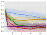
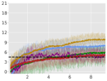
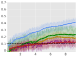
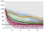
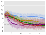
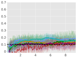
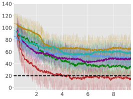
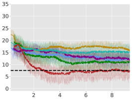
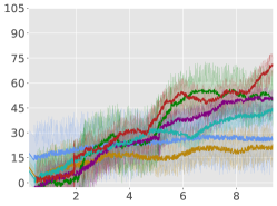
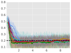
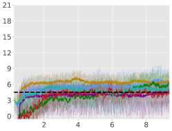
For each environment, we train an agent for steps, and for every steps, we instantiate 10 evaluation trajectories with the current (deterministic) policy. For each of these trajectories, we calculate the trajectory average reward for the next steps and finally report the total average-reward as the mean of these 10 trajectories. Learning curves for the algorithms are compiled in Figure 1 (for Point-Circle, Point-Gather, and Ant-Circle see Appendix A.6).
5.2 Performance Analysis
From Figure 1, we can see that ACPO is able to improve the reward objective while having approximate constraint satisfaction on all tasks. In particular, ACPO is the only algorithm that best learns almost-constraint-satisfying maximum average-reward policies across all tasks: in a simple Gather environment, ACPO is able to almost exactly track the cost constraint values to within the given threshold ; however, for the high dimensional Grid and Bottleneck environments we have more constraint violations due to complexity of the policy behavior. Regardless, in these environments, ACPO still outperforms all other baselines.
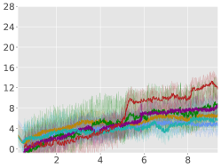
ACPO vs. CPO/PCPO. For the Point-Gather environment (see Figure 4), we see that initially ACPO and CPO/PCPO give relatively similar performance, but eventually ACPO improves over CPO and PCPO by 52.5% and 36.1% on average-rewards respectively. This superior performance does not come with more constraint violation. The Ant-Gather environment particularly brings out the effectiveness of ACPO where it shows 41.1% and 61.5% improvement over CPO and PCPO respectively, while satisfying the constraint. In the high dimensional Bottleneck and Grid environments, ACPO is particularly quick at optimizing for low constraint violations, while improving over PCPO and CPO in terms of average-reward.
ACPO vs Lagrangian ATRPO/PPO. One could suppose to use the state of the art unconstrained policy optimization algorithms with a Lagrangian formulation to solve the average-rewards CMDP problem in consideration, but we see that such an approach, although principled in theory, does not give satisfactory empirical results. This can be particularly seen in the Ant-Circle, Ant-Gather, Bottleneck, and Grid environments, where Lagrangian ATRPO and PPO give the least rewards, while not even satisfying the constraints. If ATRPO and PPO were used with constraints ignored, one would see higher rewards but even worse constraint violations, which are not useful.
ACPO vs BVF-PPO. BVF-PPO is a whole different formulation than the other baselines, as it translates the cumulative cost constraints into state-based constraints, which results in an almost-safe policy improvement method which maximizes returns at every step. However, we see that this approach fails to satisfy the constraints even in the moderately difficult Ant Gather environment, let alone the high dimensional Bottleneck and Grid environments.
5.3 Dependence of the Recovery Regime
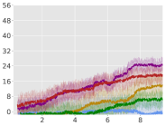
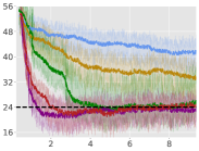

In Equation (16) we introduced a hyperparameter , which provides for an intuitive trade-off as follows: either we purely decrease the constraint violations (), or we decrease the average-reward (), which consequently decreases the constraint violation. The latter formulation is principled in that if we decrease rewards, we are bound to decrease constraints violation due to the nature of the environments. Figure 2 shows the experiments we conducted with varying . With , we obtain the same recovery scheme as that of (Achiam et al., 2017). Our results show that this scheme does not lead to the best performance, and that and perform the best across all tasks. See Appendix A.6 for a detailed study.
6 Conclusions
In this paper, we studied the problem of learning policies that maximize average-rewards for a given CMDP with average-cost constraints. We showed that the current algorithms with constraint violation bounds for the discounted setting do not generalize to the average setting. We then proposed a new algorithm, the Average-Constrained Policy Optimization (ACPO) that is inspired by the TRPO class of algorithms but based on theoretical sensitivity-type bounds for average-CMDPs we derive, and use in designing the algorithm. Our experimental results on a range of OpenAI Gym environments (including some high dimensional ones) show the effectiveness of ACPO on ACMDP RL problems, as well as its superior empirical performance vis-a-vis some current alternatives. A direction for future work is implementation of ACPO to fully exploit the parallelization potential.
Impact: This paper not only advances the field of RL theory and algorithms but also introduces a practical and scalable algorithm (supported by theory) that is of utility in many fields including LLMs, Diffusion Models, and robotic control. Currently, algorithms such as PPO are adapted for use simply because of lack of alternatives.
References
- Abounadi et al. (2001) Abounadi, J., Bertsekas, D., and Borkar, V. S. Learning algorithms for markov decision processes with average cost. SIAM Journal on Control and Optimization, 40(3):681–698, 2001.
- Achiam (2017) Achiam, J. UC Berkeley CS 285 (Fall 2017), Advanced Policy Gradients, 2017. URL: http://rail.eecs.berkeley.edu/deeprlcourse-fa17/f17docs/lecture_13_advanced_pg.pdf. Last visited on 2020/05/24.
- Achiam et al. (2017) Achiam, J., Held, D., Tamar, A., and Abbeel, P. Constrained policy optimization. In Proceedings of the 34th International Conference on Machine Learning-Volume 70, pp. 22–31. JMLR. org, 2017.
- Achiam et al. (2023) Achiam, J., Adler, S., Agarwal, S., Ahmad, L., Akkaya, I., Aleman, F. L., Almeida, D., Altenschmidt, J., Altman, S., Anadkat, S., et al. Gpt-4 technical report. arXiv preprint arXiv:2303.08774, 2023.
- Agnihotri et al. (2019) Agnihotri, A., Saraf, P., and Bapnad, K. R. A convolutional neural network approach towards self-driving cars. In 2019 IEEE 16th India Council International Conference (INDICON), pp. 1–4, 2019. doi: 10.1109/INDICON47234.2019.9030307.
- Akkaya et al. (2019) Akkaya, I., Andrychowicz, M., Chociej, M., Litwin, M., McGrew, B., Petron, A., Paino, A., Plappert, M., Powell, G., Ribas, R., et al. Solving rubik’s cube with a robot hand. arXiv preprint arXiv:1910.07113, 2019.
- Altman (1999) Altman, E. Constrained Markov decision processes, volume 7. CRC Press, 1999.
- Aractingi et al. (2023) Aractingi, M., Léziart, P.-A., Flayols, T., Perez, J., Silander, T., and Souères, P. Controlling the solo12 quadruped robot with deep reinforcement learning. scientific Reports, 13(1):11945, 2023.
- Bhatnagar & Lakshmanan (2012) Bhatnagar, S. and Lakshmanan, K. An Online Actor–Critic Algorithm with Function Approximation for Constrained Markov Decision Processes. https://doi.org/10.1007/s10957-012-9989-5, 2012. [Accessed 08-10-2023].
- Borkar (1988) Borkar, V. S. A convex analytic approach to markov decision processes. Probability Theory and Related Fields, 78(4):583–602, 1988.
- Calvo-Fullana et al. (2023) Calvo-Fullana, M., Paternain, S., Chamon, L. F., and Ribeiro, A. State augmented constrained reinforcement learning: Overcoming the limitations of learning with rewards. IEEE Transactions on Automatic Control, 2023.
- Chen et al. (2022) Chen, L., Jain, R., and Luo, H. Learning infinite-horizon average-reward Markov decision process with constraints. In Chaudhuri, K., Jegelka, S., Song, L., Szepesvari, C., Niu, G., and Sabato, S. (eds.), Proceedings of the 39th International Conference on Machine Learning, volume 162 of Proceedings of Machine Learning Research, pp. 3246–3270. PMLR, 17–23 Jul 2022. URL https://proceedings.mlr.press/v162/chen22i.html.
- Cho & Meyer (2001) Cho, G. E. and Meyer, C. D. Comparison of perturbation bounds for the stationary distribution of a markov chain. Linear Algebra and its Applications, 335(1-3):137–150, 2001.
- Doyle (2009) Doyle, P. G. The kemeny constant of a markov chain. arXiv preprint arXiv:0909.2636, 2009.
- Gao et al. (2018) Gao, Y., Xu, H., Lin, J., Yu, F., Levine, S., and Darrell, T. Reinforcement learning from imperfect demonstrations. arXiv preprint arXiv:1802.05313, 2018.
- Garcia & Fernandez (2015) Garcia, J. and Fernandez, F. A comprehensive survey on safe reinforcement learning. Journal of Machine Learning Research, 16(1):1437–1480, 2015.
- Hordijk & Kallenberg (1979) Hordijk, A. and Kallenberg, L. Linear programming and markov decision chains. Management Science, 25(4):352–362, 1979.
- Hu et al. (2022) Hu, H., Liu, Z., Chitlangia, S., Agnihotri, A., and Zhao, D. Investigating the impact of multi-lidar placement on object detection for autonomous driving. In Proceedings of the IEEE/CVF Conference on Computer Vision and Pattern Recognition (CVPR), pp. 2550–2559, June 2022.
- Hunter (2005) Hunter, J. J. Stationary distributions and mean first passage times of perturbed markov chains. Linear Algebra and its Applications, 410:217–243, 2005.
- Hunter (2014) Hunter, J. J. Mathematical techniques of applied probability: Discrete time models: Basic theory, volume 1. Academic Press, 2014.
- Kakade & Langford (2002) Kakade, S. and Langford, J. Approximately optimal approximate reinforcement learning. In International Conference on Machine Learning, volume 2, pp. 267–274, 2002.
- Kemeny & Snell (1960) Kemeny, J. and Snell, I. Finite Markov Chains. Van Nostrand, New Jersey, 1960.
- Levene & Loizou (2002) Levene, M. and Loizou, G. Kemeny’s constant and the random surfer. The American mathematical monthly, 109(8):741–745, 2002.
- Levine et al. (2016) Levine, S., Finn, C., Darrell, T., and Abbeel, P. End-to-end training of deep visuomotor policies. Journal of Machine Learning Research, 17(1):1334–1373, 2016.
- Liao et al. (2022) Liao, P., Qi, Z., Wan, R., Klasnja, P., and Murphy, S. A. Batch policy learning in average reward markov decision processes. The Annals of Statistics, 50(6):3364–3387, 2022.
- Ma et al. (2021) Ma, X., Tang, X., Xia, L., Yang, J., and Zhao, Q. Average-reward reinforcement learning with trust region methods. arXiv preprint arXiv:2106.03442, 2021.
- Manne (1960) Manne, A. S. Linear programming and sequential decisions. Management Science, 6(3):259–267, 1960.
- Mnih et al. (2015) Mnih, V., Kavukcuoglu, K., Silver, D., Rusu, A. A., Veness, J., Bellemare, M. G., Graves, A., Riedmiller, M., Fidjeland, A. K., Ostrovski, G., et al. Human-level control through deep reinforcement learning. nature, 518(7540):529–533, 2015.
- Moskovitz et al. (2023) Moskovitz, T., Singh, A. K., Strouse, D., Sandholm, T., Salakhutdinov, R., Dragan, A. D., and McAleer, S. Confronting reward model overoptimization with constrained rlhf. arXiv preprint arXiv:2310.04373, 2023.
- Rajeswaran et al. (2017) Rajeswaran, A., Kumar, V., Gupta, A., Vezzani, G., Schulman, J., Todorov, E., and Levine, S. Learning complex dexterous manipulation with deep reinforcement learning and demonstrations. arXiv preprint arXiv:1709.10087, 2017.
- Satija et al. (2020) Satija, H., Amortila, P., and Pineau, J. Constrained Markov decision processes via backward value functions. In III, H. D. and Singh, A. (eds.), Proceedings of the 37th International Conference on Machine Learning, volume 119 of Proceedings of Machine Learning Research, pp. 8502–8511. PMLR, 13–18 Jul 2020. URL https://proceedings.mlr.press/v119/satija20a.html.
- Schulman et al. (2015) Schulman, J., Levine, S., Abbeel, P., Jordan, M., and Moritz, P. Trust region policy optimization. In International Conference on Machine Learning, pp. 1889–1897, 2015.
- Schulman et al. (2016) Schulman, J., Moritz, P., Levine, S., Jordan, M., and Abbeel, P. High-dimensional continuous control using generalized advantage estimation. International Conference on Learning Representations (ICLR), 2016.
- Schulman et al. (2017) Schulman, J., Wolski, F., Dhariwal, P., Radford, A., and Klimov, O. Proximal policy optimization algorithms. arXiv preprint arXiv:1707.06347, 2017.
- Silver et al. (2017) Silver, D., Schrittwieser, J., Simonyan, K., Antonoglou, I., Huang, A., Guez, A., Hubert, T., Baker, L., Lai, M., Bolton, A., et al. Mastering the game of go without human knowledge. nature, 550(7676):354–359, 2017.
- Song et al. (2020) Song, H. F., Abdolmaleki, A., Springenberg, J. T., Clark, A., Soyer, H., Rae, J. W., Noury, S., Ahuja, A., Liu, S., Tirumala, D., et al. V-mpo: on-policy maximum a posteriori policy optimization for discrete and continuous control. International Conference on Learning Representations, 2020.
- Tessler et al. (2019) Tessler, C., Mankowitz, D. J., and Mannor, S. Reward constrained policy optimization. International Conference on Learning Representation (ICLR), 2019.
- Tibshirani (2017) Tibshirani, R. J. Dykstra’s algorithm, admm, and coordinate descent: Connections, insights, and extensions. Advances in Neural Information Processing Systems, 30, 2017.
- Todorov et al. (2012) Todorov, E., Erez, T., and Tassa, Y. Mujoco: A physics engine for model-based control. In 2012 IEEE/RSJ International Conference on Intelligent Robots and Systems, pp. 5026–5033. IEEE, 2012.
- Vinitsky et al. (2018) Vinitsky, E., Kreidieh, A., Le Flem, L., Kheterpal, N., Jang, K., Wu, F., Liaw, R., Liang, E., and Bayen, A. M. Benchmarks for reinforcement learning in mixed-autonomy traffic. In Proceedings of Conference on Robot Learning, pp. 399–409, 2018.
- Vinyals et al. (2019) Vinyals, O., Babuschkin, I., Czarnecki, W. M., Mathieu, M., Dudzik, A., Chung, J., Choi, D. H., Powell, R., Ewalds, T., Georgiev, P., et al. Grandmaster level in starcraft ii using multi-agent reinforcement learning. Nature, 575(7782):350–354, 2019.
- Vuong et al. (2019) Vuong, Q., Zhang, Y., and Ross, K. W. Supervised policy update for deep reinforcement learning. In International Conference on Learning Representation (ICLR), 2019.
- Wan et al. (2021) Wan, Y., Naik, A., and Sutton, R. S. Learning and planning in average-reward markov decision processes. In International Conference on Machine Learning, pp. 10653–10662. PMLR, 2021.
- Wei et al. (2021) Wei, C.-Y., Jahromi, M. J., Luo, H., and Jain, R. Learning infinite-horizon average-reward mdps with linear function approximation. In International Conference on Artificial Intelligence and Statistics, pp. 3007–3015. PMLR, 2021.
- Wu et al. (2017) Wu, Y., Mansimov, E., Grosse, R. B., Liao, S., and Ba, J. Scalable trust-region method for deep reinforcement learning using kronecker-factored approximation. In Advances in neural information processing systems (NIPS), pp. 5285–5294, 2017.
- Yang et al. (2020) Yang, T.-Y., Rosca, J., Narasimhan, K., and Ramadge, P. J. Projection-based constrained policy optimization. In International Conference on Learning Representation (ICLR), 2020.
- Zhang et al. (2021) Zhang, S., Wan, Y., Sutton, R. S., and Whiteson, S. Average-reward off-policy policy evaluation with function approximation. arXiv preprint arXiv:2101.02808, 2021.
- Zhang & Ross (2020) Zhang, Y. and Ross, K. Average reward reinforcement learning with monotonic policy improvement. Preprint, 2020.
Appendix A Appendix
A.1 Proofs
Lemma A.1 (Trivialization of Discounted Criterion Bounds).
Consider the policy performance bound of (Achiam et al., 2017), which says that for any two stationary policies and :
| (17) |
where . Then, the right hand side times goes to negative infinity as .
Proof.
Since approaches the stationary distribution as , we can multiply the right hand side of (17) by and take the limit which gives us:
Here . The first equality is a standard result of . ∎
See 3.1
Proof.
We directly expand the right-hand side using the definition of the advantage function and Bellman equation, which gives us:
Analyzing , since is a stationary distribution:
Therefore, . Hence, proved. ∎
See 3.2
Proof.
| (from Lemma 3.1) | ||||
| (Holder’s inequality) | ||||
∎
See 3.3
Proof.
This proof takes ideas from Markov chain perturbation theory in (Cho & Meyer, 2001; Hunter, 2005; Zhang & Ross, 2020). Firstly we state a standard result with
Denoting the fundamental matrix of the Markov chain and the mean first passage time matrix , and right multiplying the above by we have,
| (18) | ||||
| (submultiplicative property) | ||||
We know that and from (Hunter, 2014), we can write using the eigenvalues of the underlying as
For , we refer to the result by (Zhang & Ross, 2020), and provide the proof for completeness below.
Combining these inequalities of and , we get the desired result. ∎
A.2 Performance and Constraint Bounds of Trust Region Approach
Consider the trust region formulation in Equation (10). To prove the policy performance bound when the current policy is infeasible (i.e., constraint-violating), we prove the KL divergence between and for the KL divergence projection, along with other lemmas. We then prove our main theorem for the worst-case performance degradation.
Lemma A.2.
For a closed convex constraint set, if we have a constraint satisfying policy and the KL divergence of the ‘Improve’ step is upper bounded by step size , then after KL divergence projection of the ‘Project’ step we have
Proof.
We make use of the fact that Bregman divergence (hence, KL divergence) projection onto the constraint set () exists and is unique. Since is safe, we have in the constraint set, and is the projection of onto the constraint set. Using the projection inequality, we have
| () |
Since KL divergence is asymptotically symmetric when updating the policy within a local neighbourhood (), we have
∎
Lemma A.3.
For a closed convex constraint set, if we have a constraint violating policy and the KL divergence of the first step is upper bounded by step size , then after KL divergence projection of the second step we have
where , with as the gradient of the cost advantage function corresponding to constraint , and as the Hessian of the KL divergence constraint. 222For any .
Proof.
Let the sublevel set of cost constraint function for the current infeasible policy be given as:
This implies that the current policy lies in . The constraint set onto which is projected onto is given by: Let be the projection of onto
Note that the Bregman inequality of Lemma A.2 holds for any convex set in . This implies since and are both in , which is also convex since the constraint functions are convex. Using the Three-point Lemma 333For any , the Bregman divergence identity: , for polices and , with , we have
| (19) |
If the constraint violations of the current policy are small, i.e., is small for all , then can be approximated by a second order expansion. We analyze for any constraint and then bound it over all the constraints. As before we overload the notation with to write. For any constraint , we can write as the expected KL divergence if projection was onto the constraint set of i.e.
where the second equality is a result of the trust region guarantee (see (Schulman et al., 2015) for more details). Finally we invoke the projection result from (Achiam, 2017) which uses Dykstra’s Alternating Projection algorithm from (Tibshirani, 2017) to bound this projection, i.e., .
And since is small, we have given . Thus, . Combining all of the above, we have ∎
See 3.6
Proof.
Since , is feasible. The objective value is 0 for . The bound follows from Equation (7) and Equation (9) where the average KL i.e. is bounded by from Lemma A.3.
Similar to Corollary 3.5, expressions for the auxiliary cost constraints also follow immediately as the second result.
Remark A.4.
Remark If we look at proof as given by (Zhang & Ross, 2020) in Section 5 of their paper, with the distinction now that is replaced by , we have the same result. Our worse bound is due to the constrained nature of our setting, which is intuitive in the sense that for the sake of satisfying constraints, we undergo a worse worst-case performance degradation.
∎
A.3 Approximate ACPO
A.3.1 Policy Recovery Routine
As described in Section 4.2, we need a recovery routine in case the updated policy is not approximate constraint satisfying. In this case, the optimization problem is inspired from a simple trust region approach by (Schulman et al., 2015). Since we only deal with one constraint in the practical implementation of ACPO, the recovery rule is obtained by solving the following problem:
Let , then the dual function is given by: . Now,
obtained above should satisfy the trust-region constraint:
Therefore, the update rule in case of infeasibility takes the form . We augment this rule with the gradient of the reward advantage function as well, so the final recovery is
A.3.2 Line Search
Because of approximation error, the proposed update may not satisfy the constraints in Eq. (10). Constraint satisfaction is enforced via line search, so the final update is
where is the backtracking coefficient and is the smallest integer for which satisfies the constraints in Equation 10. Here, is a finite backtracking budget; if no proposed policy satisfies the constraints after backtracking steps, no update occurs.
A.4 Practical ACPO
As explained in Section 4, we use the below problem formulation, which uses first-order Taylor approximation on the objective and second-order approximation on the KL constraint 444The gradient and first-order Taylor approximation of at is zero. around , given small :
| (20) | ||||
| s.t. |
where
Similar to the work of (Achiam et al., 2017), , , and can be approximated using samples drawn from the policy . The Hessian is identical to the Hessian used by (Achiam et al., 2017) and (Zhang & Ross, 2020). However, the definitons and ’s are different since they include the average reward advantage functions, .
Since rewards and cost advantage functions can be approximated independently, we use the framework of (Zhang & Ross, 2020) to do so. We describe the process of estimation of rewards advantage function, and the same procedure can be used for the cost advantage functions as well. Specifically, first approximate the average-reward bias and then use a one-step TD backup to estimate the action-bias function. Concretely, using the average reward Bellman equation gives
| (21) |
This expression involves the average-reward bias , which we can approximated using the standard critic network . However, in practice we use the average-reward version of the Generalized Advantage Estimator (GAE) from (Schulman et al., 2016), similar to (Zhang & Ross, 2020). Hence, we refer the reader to that paper for detailed explanation, but provide an overview below for completeness.
Let denote the estimated average reward. The Monte Carlo target for the average reward value function is and the bootstrapped target is .
The Monte Carlo and Bootstrap estimators for the average reward advantage function are:
We can similarly extend the GAE to the average reward setting:
| (22) |
and set the target for the value function to .
A.5 Experimental Details
For detailed explanation of Point-Circle, Point-Gather, Ant-Circle, and Ant-Gather tasks, please refer to (Achiam et al., 2017). For detailed explanation of Bottleneck and Grid tasks, please refer to (Vinitsky et al., 2018). For the simulations in the Gather and Circle tasks, we use neural network baselines with the same architecture and activation functions as the policy networks. For the simulations in the Grid and Bottleneck tasks, we use linear baselines. For all experiments we use Gaussian neural policies whose outputs are the mean vectors and variances are separate parameters to be learned. Seeds used for generating evaluation trajectories are different from those used for training.
For comparison of different algorithms, we make use of CPO, PCPO, ATRPO, and PPO implementations taken from https://github.com/rll/rllab and https://github.com/openai/safety-starter-agents. Even the hyperparameters are selected so as to showcase the best performance of other algorithms for fair comparison. The choice of the hyperparameters given below is inspired by the original papers since we wanted to understand the performance of the average reward case.
We use settings which are common in all open-source implementations of the algorithms, such as normalizing the states by the running mean and standard deviation before being fed into the neural network and similarly normalizing the advantage values (for both rewards and constraints) by their batch means and standard deviations before being used for policy updates. Table 1 summarizes the hyperparameters below.
| Hyperparameter | PPO/ATRPO | CPO/PCPO/ACPO |
| No. of hidden layers | 2 | 2 |
| Activation | ||
| Initial log std | -0.5 | -1 |
| Batch size | 2500 | 2500 |
| GAE parameter (reward) | 0.95 | 0.95 |
| GAE parameter (cost) | N/A | 0.95 |
| Trust region step size | ||
| Learning rate for policy | ||
| Learning rate for reward critic net | ||
| Learning rate for cost critic net | N/A | |
| Backtracking coeff. | 0.75 | 0.75 |
| Max backtracking iterations | 10 | 10 |
| Max conjugate gradient iterations | 10 | 10 |
| Recovery regime parameter | N/A | 0.75 |
For the Lagrangian formulation of ATRPO and PPO, note that the original papers do not provide any blueprint for formulating the Lagrangian, and even CPO and PCPO use unconstrained TRPO for benchmarking. However, we feel that this is unfair to these algorithms as they can possibly perform better with a Lagrangian formulation in an average-reward CMDP setting. To this extent, we introduced a Lagrangian parameter that balances the rewards and constraints in the final objective function. More specifically, Equation (13) for a single constraint now becomes
| (23) |
Note.
The authors of the ATRPO and PPO do not suggest any principled approach for finding an optimal . Hence, the choice of the Lagrangian parameter is completely empirical and is selected such that these algorithms achieve maximum rewards while satisfying the constraints. Also see in Figure 1, for Ant-Gather, Bottleneck, and Grid environments, where the constraints cannot be satisfied for any value of , we include the results for a specific value of for illustrative purposes, as detailed in Table 2.
| Algorithm | Point-Gather | Ant-Circle | Ant-Gather | Bottleneck | Grid |
|---|---|---|---|---|---|
| ATRPO | 0.50 | 0.60 | 0.45 | 0.50 | 0.45 |
| PPO | 0.55 | 0.50 | 0.50 | 0.50 | 0.60 |
A.6 Experimental Addendum
A.6.1 Environments
All environments tested on are illustrated in Figure 3, along with a detailed description of each.



A.6.2 Learning Curves
Due to space restrictions, we present the learning curves for the remaining environments in Figure 4.
Average Rewards:
Average Constraint values: 
A.6.3 Recovery Regime Revisited
In Subsection 5.3, we studied the effect of the hyperparameter for only one task. Figure 5 shows the performance of ACPO with different values of in various environments.
Rewards:


Constraint values: 
