Accuracy of Stellar Mass-to-light Ratios of Nearby Galaxies in the Near-Infrared
Abstract
Future satellite missions are expected to perform all-sky surveys, thus providing the entire sky near-infrared spectral data and consequently opening a new window to investigate the evolution of galaxies. Specifically, the infrared spectral data facilitate the precise estimation of stellar masses of numerous low-redshift galaxies. We utilize the synthetic spectral energy distribution (SED) of 2853 nearby galaxies drawn from the DustPedia (435) and Stripe 82 regions (2418). The stellar mass-to-light ratio () estimation accuracy over a wavelength range of m is computed through the SED fitting of the multi-wavelength photometric dataset, which has not yet been intensively explored in previous studies. We find that the scatter in is significantly larger in the shorter and longer wavelength regimes due to the effect of the young stellar population and the dust contribution, respectively. While the scatter in approaches its minimum ( dex) at m, it remains sensitive to the adopted star formation history model. Furthermore, demonstrates weak and strong correlations with the stellar mass and the specific star formation rate (SFR), respectively. Upon adequately correcting the dependence of on the specific SFR, the scatter in the further reduces to dex at m. This indicates that the stellar mass can be estimated with an accuracy of dex with a prior knowledge of SFR, which can be estimated using the infrared spectra obtained with future survey missions.
1 Introduction
The stellar mass is one of the most fundamental parameters that offer crucial insights into the formation and evolution of galaxies. Furthermore, it helps probe the mass assembly history of galaxies through the stellar mass function (e.g., Madau & Dickinson, 2014). In addition, its correlations with other physical properties of galaxies (e.g., metallicity, size, halo mass, and the mass of the central supermassive black hole) help facilitate the detailed evolution of galaxies (e.g., Maiolino & Mannucci, 2019; Wechsler & Tinker, 2018; Kormendy & Ho, 2013; Conselice, 2014). Therefore, robust estimations of the stellar mass are crucial for understanding the detailed evolution of the galaxy.

The stellar mass for a large number of samples has conventionally relied on broad-band photometry, assuming a constant mass-to-light ratio () for a given broad-band filter. In line with these practices, , known to depend on the stellar age, metallicity, initial mass function (IMF), and dust extinction, was theoretically or semi-empirically derived using the stellar population model (e.g., Larson & Tinsley, 1978; Bell et al., 2003; Bruzual & Charlot, 2003; Zibetti et al., 2009; Taylor et al., 2011). As those properties cannot be directly measured with ease, a color index has been widely used as a secondary parameter to infer . While the accuracy of this method strongly depends on the effective wavelength of the filter, the scatter in is dex (e.g., Bell et al., 2003; Zibetti et al., 2009; Taylor et al., 2011; Into & Portinari, 2013; Roediger & Courteau, 2015). Note that this scatter does not account for systematics arising from uncertainties in the stellar population models, which can be up to dex (e.g., Conroy, 2013; Hon et al., 2022). This effect, specifically in NIR (m), is examined in another study (Lee et al., submitted). Alternatively, is often estimated using spectral energy distributions (SED) constructed from multiple broad-band photometric data (Conroy, 2013). In this approach, synthetic SEDs are modeled with varying star formation history (SFH), which can introduce additional uncertainty in the stellar mass estimation. This uncertainty becomes more significant when photometric coverage is limited.


Photometric data from the near-infrared (NIR) spectral regions are particularly useful to robustly estimate the stellar mass, as it is minimally affected by the dust attenuation and the ratio is less sensitive to the stellar age compared to those from the UV/optical data (Into & Portinari, 2013). However, intermediate-age stars such as those on the thermally pulsating asymptotic giant branch (TP-AGB) can significantly contribute to the fluxes in the NIR (e.g., Meidt et al., 2012), underscoring that the accuracy of the stellar mass estimation is closely tied to the reliability of the stellar population models in the NIR (e.g., Taylor et al., 2011; Conroy, 2013). For example, -band photometric data combined with can be a powerful tool for the stellar mass estimation in the local Universe (e.g., Bell et al., 2003). In addition, NIR photometric data predominantly extracted from the Spitzer Space Telescope (Werner et al., 2004) and the WISE mission (Wright et al., 2010) contributed significantly to the stellar mass estimation of relatively nearby galaxies (e.g., Meidt et al., 2014; Querejeta et al., 2015; Jarrett et al., 2023). Notably, NIR-based above m are easily contaminated by the emission lines and continuum originating from the warm dust, which requires empirical corrections using the NIR colors (e.g., W1-W2 or IRAC1-IRAC2). However, the complex contributions from the 3.3 m polycyclic aromatic hydrocarbon (PAH) emission to the W1 and IRAC1 bands complicate the dust-contamination corrections solely based on NIR colors (e.g., Lee et al., 2012; Yamada et al., 2013; Inami et al., 2018; Lai et al., 2020), potentially introducing systematic uncertainties on the stellar mass estimations. Collectively, these effects can limit the accuracy of the stellar mass estimations based on NIR broad-band photometric data.
Upcoming satellite missions, including The Spectro-Photometer for the History of the Universe, Epoch of Reionization and Ices Explorer (SPHEREx), are poised to enrich our understanding of the Universe (Korngut et al. 2018; Crill et al. 2020). In particular, SPHEREx will conduct an all-sky survey with linear variable filters, providing the all-sky spectral data spanning a wavelength range of m with spectral resolutions of (Doré et al., 2016; Crill et al., 2020). This extensive dataset will enable us to estimate the stellar mass of numerous galaxies, which is crucial to understanding the galaxy evolution in the nearby Universe. Furthermore, leveraging its wide wavelength coverage and spectral capabilities, this NIR dataset is expected to facilitate precise stellar-mass estimations. However, the NIR spectral range (1–5 µm) remains relatively underexplored owing to limited observational data Brown et al. (2014).
Based on the above backgrounds, we investigate the within the spectral range of m, covered by SPHEREx, which will provide the low spectral resolution () data. For that purpose, we utilize the synthetic SED obtained from the SED fitting of the multi-wavelength data of nearby galaxies adopted from literature. The sample selection and adopted dataset are summarized in Section 2. The NIR-based estimations are calculated in Section 3. The estimation accuracy of the obtained ratio is described in Section 4. In Section 5, we summarize the conclusions of this study. Throughout the paper, we adopt the cosmological parameters: km and . All magnitudes are given in the Vega system.
2 Sample and Data
2.1 Sample Selection
To utilize the SED derived from the observed photometric dataset, we first employ the sample from the DustPedia (Davies et al., 2017; Clark et al., 2018). The multi-wavelength dataset of the DustPedia spanning the UV to far-infrared (FIR) enables robust estimations of both stellar population and dust properties through SED fitting with the Code Investigating GALaxy Emission (CIGALE) code (Boquien et al., 2019). This characteristic makes the DustPedia sample ideal for our study (Nersesian et al., 2019). The DustPedia constructed the SEDs based on the aperture-matched photometry on the 42 bands data covering UV to sub-mm, obtained from the Hershel observation, along with the archival observations from the GALEX, SDSS, 2MASS, WISE, Spitzer, and Planck. The original DustPedia sample contains 875 nearby galaxies with Mpc. However, this DustPedia sample is slightly biased toward low-mass galaxies () because of their proximity.
To compensate for this limitation, we additionally adopt a sample of nearby () massive galaxies from Li et al. (2023), which employed data from the SDSS Stripe 82 region (S82). Li et al. (2023) conducted the sophisticated photometry on the multi-wavelength imaging data of 2685 massive galaxies (). As the initial sample selection was based on stellar mass estimates from the GALEX–SDSS–WISE Legacy Catalog (GSWLC-2; Salim et al., 2018), a small fraction of the S82 sample finally shows . These data encompassed UV, optical, NIR, MIR, and FIR data obtained from GALEX, SDSS, 2MASS, WISE, and Herschel-SPIRE, respectively. The matched-aperture and profile-fitting photometry were applied for the shorter-wavelength bands ranging from UV to W2 and the longer-wavelength bands, respectively. In addition, multi-band imaging decomposition was carefully performed to accurately remove the contribution from neighboring galaxies or foreground stars. These procedures resulted in reliable flux measurements and precise estimations of the uncertainties of the multi-wavelength dataset. From the comparison with the photometric data of GALEX, SDSS, and 2MASS extended source catalogs (Jarrett et al., 2000), Li et al. (2023) showed that their measurements agree within mag in the UV, optical, and NIR bands. However, the photometric measurements of Li et al. (2023) are systematically brighter ( mag) than those in 2MASS point source catalog (Cutri et al., 2003) and ALLWISE, in which the photometric data were originally estimated from a PSF-fitting method. Notably, these systematic discrepancies are significantly reduced up to mag when compared with the unWISE catalog (Lang et al., 2016).


2.2 SED Fitting
For the S82 sample, stellar and dust masses are drawn from Li et al. (2023). These parameters were obtained via SED fitting using the CIGALE. In this SED fitting process, the stellar SED was modeled using the simple stellar population (SSP) from Bruzual & Charlot (2003). The stellar population was modeled with a double-exponential SFH, comprising an old stellar population with an age of 12 Gyr and a young stellar population with an age range from 10 to 5000 Myr. The stellar emission was modeled with metallicities of . The IMF of Chabrier (2003) was adopted. In addition, the starburst attenuation curve from Calzetti et al. (2000) with a modification of the power-law slope was adopted to account for the dust attenuation in the SED fitting.
Dust emission is modeled with , (fixed), . Here, denotes the minimum radiation field from the stars; represents the mass fraction of PAHs; indicates the mass fraction of dust illuminated from the minimum to maximum radiation field. , the power-law slope of the dust continuum over the IR wavelength, is fixed to 2. Nebular emission lines were also included (Inoue, 2011). The AGN component modeled with Fritz et al. (2006) was incorporated. Here, the AGN fraction () was calculated as the ratio of the AGN luminosity to the total IR luminosity estimated within m.
Whereas the SED fitting with the CIGALE was also applied to the DustPedia sample (Jones et al., 2013; Nersesian et al., 2019), parameters for the stellar population and dust modeling significantly differ from those of Li et al. (2023). In addition, contrary to the S82 sample, the SED fitting of the DustPedia sample did not consider any AGN components. To avoid possible systematics due to these factors, we perform the SED fitting on the DustPedia dataset. To maintain consistency, we adopt the same fitting parameters and bandpasses used for the S82 dataset. We exclude the photometric data contaminated by artifacts or nearby sources, as well as data obtained from the imaging data that partially covers the target source (Clark et al., 2018). To secure accurate stellar mass measurements from the SED fitting, samples lacking flux measurements in the optical band () are further discarded. The systematic effects due to the discrepancy in the fitting parameters between the original DustPedia study (Nersesian et al., 2019) and this study are further discussed in Appendix A.
We discard the targets with a reduced value exceeding 2 to ensure reliable assessments of the stellar and dust properties. Furthermore, following the recipe from Li et al. (2023), the AGNs defined as were excluded, as the flux contribution from the AGN can introduce additional uncertainties. This results in the final samples containing 435 and 2418 galaxies from the DustPedia and S82, respectively. Throughout this study, we utilize the synthetic SEDs obtained from the best fit for magnitude estimations across various filters and wavelengths. The goodness-of-fit, particularly in NIR regions, is examined in Appendix B. The stellar masses derived from the SED fitting agree with those of GALEX-SDSS-WISE Legacy Catalog 2 (GSWLC-2; Salim et al., 2018) with dex (Li et al., 2023). However, a moderate difference is observed in the star formation rate when compared to GSWLC-2 ( dex). As described in Li et al. (2023), this discrepancy arises from the differences in the methods of photometric measurements, particularly in the mid- and far-infrared bands.


Figure 1 illustrates the distributions of stellar and dust masses determined from the SED fitting process, demonstrating the complementary characteristics of the two subsamples in the two-parameter space. Furthermore, our sample covers a wide range of SFR at a given stellar mass, from the star-forming main sequence to relatively quiescent galaxies, which is crucial to investigate the variations in the ratio with various properties of galaxies (Fig. 2).
3 Results
3.1 Mass-to-Light Ratio in Broadband Photometry
Conventionally, stellar-mass estimations in the NIR band (m) have been based on broadband photometry obtained from the Spitzer Space Telescope and the WISE mission. As the first step of our analysis, we compute at commonly used broadband filters in the NIR (e.g., IRAC1 and W1). Figure 3 shows at IRAC1 and W1 using the stellar and total luminosities. Overall, we can estimate the stellar mass with an accuracy of dex solely with the NIR data, which is consistent with the previous studies (e.g. Meidt et al., 2014; Kettlety et al., 2018; Jarrett et al., 2023).111It is worthwhile to note that this accuracy is calculated relative to the stellar mass derived from the SED fitting performed using the parameterized SFH, potentially introducing a zero-point offset of up to dex. This bias, however, is not considered in this study (e.g. Conroy, 2013; Lower et al., 2020). However, as the dust continuum and 3.3 m PAH emission can contribute to the total luminosity in those filters, the ratios calculated using the total luminosity exhibit a substantially larger scatter compared to those calculated using the stellar luminosity.
Meanwhile, considering only the stellar light, the scatter in can be significantly reduced down to dex. While the average ratio at IRAC 1 [ or ] is in good agreement with the prediction for the old stellar population (; Meidt et al. 2014; Querejeta et al. 2015), that at the W1 band [ () and (] from the total and stellar luminosity, respectively] is significantly larger than the empirically derived value for the nearby galaxies (; Jarrett et al., 2023). Note that in Jarrett et al. (2023) is derived from the W1 total luminosity. With the EAGLE simulations, Norris et al. (2016) examined the M/L distribution of simulated early-type/quiescent galaxies and found , which is in good agreement with a peak in the higher found in the distribution of (Fig. 3). While the origin of this discrepancy remains rather unclear, it can be partially attributed to differences in flux measurements across the chosen datasets. Specifically, the dedicated flux measurements of the WISE dataset obtained from Li et al. (2023) are systematically brighter by mag compared to the ALLWISE measurements based on profile-fitting results, which was used to estimate the values in Jarrett et al. (2023). Interestingly, in our study, the values calculated for W1 and IRAC1 are consistent with each other, which supports the reliability of our estimates. It is also worthwhile noting that, unlike other studies, Jarrett et al. (2023) used the observed total luminosity, instead of the stellar luminosity, to calculate the values, naturally resulting in a low .

3.2 Mass-to-Light Ratio in Spectral Data
As the NIR spectral data will be obtained through future space missions, such as SPHEREx, investigating the in these spectral elements is worthwhile. To this end, we employ 68 spectral components with a spectral resolution of 40 (i.e., , where is the bandwidth of each spectral component), covering a wavelength range of 0.755.0 m. For simplicity, the transmission curve of each spectral component is modeled using a Gaussian profile. Although this assumption does not exactly match the spectral channels of the SPHEREx, it is adequate for examining the overall trend of the ratio as a function of the wavelength.
As expected, the ratio is inversely proportional to the wavelength because the ratios in the shorter wavelengths are more sensitive to the young stellar population compared to those at the longer wavelength. However, the scatter of the ratio exhibits a U-shaped pattern. The values calculated using the total luminosity are significantly affected at longer wavelengths due to the existence of the dust continuum and PAH emission (Fig. 4). In particular, the excess in the scatter is remarkable around 3.3 m, highlighting the need for the careful removal of the PAH emission to facilitate accurate stellar mass estimations. This effect can be rigorously quantified using the spectral dataset provided by the SPHEREx mission, particularly for star-forming galaxies (e.g. Xie et al., 2018a, b; Zhang et al., 2021).


In addition, the values in the DustPedia sample are systematically smaller than those in the S82 sample. The values are known to be strongly dependent on the specific SFR (e.g., Portinari et al., 2004). The DustPedia sample tends to have a larger specific SFR than the S82 sample (see §4.2), which may be the main cause of smaller values for the DustPedia sample.
The scatter in the ratios calculated from the stellar luminosity is significantly reduced (Fig. 5). At wavelengths longer than 1m, the overall scatter ranges between 0.1 and 0.11 dex, demonstrating a weak dependence on the wavelength. This indicates that the NIR spectrum is valuable for constraining the stellar mass almost regardless of the wavelength if the dust component can be adequately removed. The values and their scatter for both subsamples are summarized in Table 1.
4 Discussion
4.1 Dust Contribution to NIR Photometry
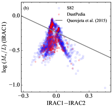
The NIR colors (IRAC1-IRAC2 or W1-W2) have been utilized to approximate the light contribution from the dust, which needs to be adequately subtracted to estimate the stellar mass precisely. The basic assumption of this procedure is that the dust continuum is intrinsically redder than the stellar continuum. According to this assumption, Querejeta et al. (2015) and Jarrett et al. (2023) demonstrated that is inversely proportional to both the IRAC1-IRAC2 and W1-W2 colors, respectively. Here, we examine the validity of this finding for our dataset. We find two sequences in the plane of and W1-W2 color for our sample (Fig. 6). In one sequence, consistent with the findings of previous studies, is mildly anti-correlated with the W1-W2 and IRAC1-IRAC2 color. Although this correlation broadly agrees with the general trend in earlier studies (e.g., Cluver et al., 2014; Jarrett et al., 2023), the observed relation between the two quantities deviates from those of previous studies. We attribute this to the fact that the photometric measurements of W1 and W2 adopted in this study are systematically brighter than the ALLWISE measurements (Li et al. 2023).

However, in another sequence, is almost independent of the W1W2 color, with a substantially large scatter. To comprehend this finding, we compare the NIR color with the ratio of the flux from the dust components to the total flux () at the W1 band. Figure 7 shows that the dust fraction at the W1 band is only weakly correlated with the W1W2 color. The hot and warm dust ( K) from the star-forming regions can naturally increase the W1W2 color (e.g., Xie et al., 2018a). Conversely, the prominent 3.3 m PAH emission can boost the flux only at the W1 band, making the W1W2 color bluer. Because the strength of the 3.3 m PAH emission is proportional to the SFR but with a significant amount of the scatter, the correlation between the W1W2 color and the dust fraction can be excessively intricate due to the competition between the dust continuum and PAH emission. This complexity cannot be quantified without a spectroscopic dataset (e.g., Yamada et al., 2013; Shim et al., 2023). A similar trend (i.e., a non-linear correlation between the dust fraction and the NIR color) is also shown in the IRAC1IRAC2 color.
As SPHEREx will provide the spectral information, the spectral color can serve as a better tracer for the dust contribution. Here, we adopt a color index between 3 m and 4 m () to avoid the strong 3.3 m emission and compare it with the flux ratio of the dust at 3 m (). We find that is strongly correlated with expressed as (Fig. 8), indicating that the dust contribution can be approximately estimated with the spectral color index in SPHEREx dataset.

4.2 Main Driver of the Scatter in
Given that the ratios can be highly affected by the stellar properties of the galaxies, adopting a second parameter is often essential for robustly estimating the stellar mass. Previous studies have extensively adopted the color term as the second parameter (e.g., Bell et al., 2003; Into & Portinari, 2013). To identify an alternative in the spectral analysis, we investigate the parameter predominantly deriving the scatter in . Initially, we find that is weakly correlated with the stellar mass itself, likely attributed to the dependence of the SFH on stellar mass. To account for this dependence, we perform a linear regression between the stellar mass and at each wavelength as follows: (see Figure 9 for an example). The fitting results as a function of the wavelength are summarized in Table 2. With this treatment, the scatter is mildly reduced by dex. Thus, overall, with the NIR spectrum, the stellar mass can be estimated with a typical uncertainty of dex (Fig. 10).
Furthermore, the ratio is tightly correlated with the SFR divided by the stellar mass, namely the specific star formation rate (sSFR). Figure 11 shows that this relation at m is well fitted with a smoothly broken power law, which is defined as:
| (1) |
where is the normalization factor [i.e., at ], is the pivot sSFR, is the power-law index at , and is the smoothness parameter, which determines the smoothness of the power-law slope change around the pivot sSFR. Note that the unit of sSFR is Gyr-1. Fitting results for various wavelengths are summarized in Table 3. This trend is rather expected from the adopted SFH with two components (old and young stellar populations) because the sSFR approximately traces the mass ratio of the old stellar population to the young stellar population. Considering this dependency, the scatter in dramatically decreases to dex (Fig. 12). This result clearly demonstrates that more precise stellar mass estimations can be achieved using the known SFR. Note that the SFR used in this analysis is an instantaneous SFR provided by the CIGALE based on the star formation history. As the commonly used SFR indicators (e.g., hydrogen recombination lines) trace the average SFR over the last Myr, the observed SFRs may differ from those provided by CIGALE to some degree, which can introduce additional uncertainty in the estimation (e.g., Byun et al., 2021).

4.3 Best Stellar Mass Indicator in NIR
Based on our calculations of under various conditions, we attempt to identify an optimal method to estimate the stellar mass based on the NIR spectral data of nearby galaxies. If the contribution of the dust emission can be adequately removed from the observed spectrum, the scatter in the ratio becomes almost independent of the wavelength. However, it is challenging to fit the PAH emissions and the dust continuum robustly, even using the NIR/MIR spectroscopic data (e.g. Xie et al., 2018a; Zhang & Ho, 2023). Therefore, if available, NIR data around a wavelength of m are preferable, as will also be presented in Lee, J. H. et al. (submitted). This is because it is relatively free from dust contamination unless the AGN component is prominent, and the resulting scatter in is smaller or comparable to that achieved using NIR data.
As outlined in the previous section (§4.2), the scatter in can be slightly reduced if the dependence of on stellar mass is considered. To this end, the stellar mass can be estimated from using the monochromatic luminosity and subsequently subjected to iterative fine-tuning. Specifically, the initial stellar mass is estimated from a constant , following which the correlation between the ratio and stellar mass can be corrected using the initial stellar mass measurement to achieve a more precise stellar-mass estimation. However, this iterative process can reduce the uncertainty by only dex. Conversely, if the SFR can be estimated based on the NIR spectral data, for example, from the fluxes of hydrogen recombination lines (e.g., Kennicutt & Evans, 2012) or 3.3 m PAH emissions (e.g. Kim et al., 2012; Lai et al., 2020; Belfiore et al., 2023), the scatter in the stellar mass estimation can be dramatically reduced based on the strong correlation between and sSFR. It is worthwhile to note that 3.3 m PAH-based SFR can be more uncertain compared to other SFR indicators (e.g., hydrogen lines, UV, and IR) as its brightness relative to IR luminosity is correlated with physical parameters of host galaxies, such as metallicity (e.g. Shim et al., 2023; Whitcomb et al., 2024). However, this correction must again follow an iterative procedure, as a prior stellar mass estimate is essential to compute the sSFR. An alternative argument is that SFR, rather than sSFR, could be used to trace . However, we find that the scatter in the correlation between SFR and is significantly larger than that for sSFR. Therefore, sSFR provides a more reliable estimate of . In conclusion, the NIR spectrophotometry provided by the SPHEREx can improve the accuracy of stellar mass estimations.
5 Conclusion
To investigate the accuracy of the ratio at the NIR continuum, we employ the synthetic SEDs of stellar populations and dust derived from the observed multi-wavelength data ranging from UV to FIR of nearby galaxies at . The SED fitting results for two subsamples from the DustPedia and the S82 regions are adopted for this purpose. The stellar masses of the sample are also calculated based on the SED fitting results. The followings are some key findings and conclusions of our study:
-
•
The ratios in the widely used NIR broadband filters (e.g., W1 and IRAC1) are heavily affected by the strength of the dust continuum and PAH emissions. Our results demonstrate that the variations in the ratio resulting from this effect cannot be easily quantified using the NIR color (e.g., W1W2 or IRAC1IRAC2) because the relative contribution between the dust continuum and PAH emission is complicated. This systematics effect can be significantly alleviated using the color index of NIR spectral data.
-
•
While in the NIR spectral range is strongly correlated with the wavelength, the scatter in as a function of the wavelength exhibits a U-shaped profile due to the dependence on the stellar age and dust features in the short and long wavelength, respectively.
-
•
If the contribution from the dust component can be adequately excluded from the NIR spectrum, the scatter in can be significantly reduced in the long wavelength region and remain nearly constant along the wavelength with a variation of dex.
-
•
demonstrates a weak correlation with the stellar mass and a strong correlation with the sSFR. If this dependency is corrected appropriately, the scatter in can be dramatically decreased up to dex. Based on these findings, we conclude that the stellar mass can be most accurately estimated using spectral data around m, combined with SFR measurements.
Appendix A Comparison with Previous Studies for the DustPedia Sample
For the DustPedia sample, the SED fitting with distinct fitting parameters was performed in the previous study (Nersesian et al., 2019). Specifically, the DustPedia sample was fitted with a flexible-delayed SFH, comprising both young ( Myr) and old ( Myr) SSPs in Nersesian et al. (2019). Among these SSPs, the old stellar population with an age range between 2 and 12 Gyr was assumed to exhibit an exponentially declining SFR, while the young stellar population was modeled with a burst or a decline of constant SFR at 200 Myr ago. The IMF of Salpeter (1955) was adopted. In addition, the dust emission was modeled using a broader range of parameters than in this study. In this appendix, we investigate systematics arising from differences in SFH and dust modeling by comparing our fitting results with those from Nersesian et al. (2019). The discrepancy in the stellar masses is nearly negligible on average [] with a scatter of dex, which may correspond to the additional uncertainty introduced by differences in SFH and IMF in the SED fitting (Fig. A1). The SFR shows a marginally larger offset and scatter [ dex; Fig. A1]. However, this uncertainty will have minimal impact on this study.


Appendix B Residuals from the SED Fitting in NIR bands
The SED model in the NIR is highly sensitive to the choice of stellar population model, particularly based on how TP-AGB stars are treated (e.g., Maraston et al., 2006). To understand the systematics of due to this fact, it is helpful to assess the goodness of fit by examining the NIR residuals. Figure A2 illustrates the residuals in the NIR bands (, W1, and W2) derived from the best SED fit. Note only the results with a signal-to-noise greater than 5 are used in the experiment. Notably, the model SEDs tend to underestimate the fluxes at , though the offsets remain within the error margin. This indicates that the NIR-based could be marginally underestimated up to dex, although this result is not definitive.

References
- Belfiore et al. (2023) Belfiore, F., Leroy, A. K., Williams, T. G., et al. 2023, A&A, 678, A129
- Bell et al. (2003) Bell, E. F., McIntosh, D. H., Katz, N., & Weinberg, M. D. 2003, ApJS, 149, 289
- Boquien et al. (2019) Boquien, M., Burgarella, D., Roehlly, Y., et al. 2019, A&A, 622, A103
- Brown et al. (2014) Brown, M. J. I., Moustakas, J., Smith, J. D. T., et al. 2014, ApJS, 212, 18
- Bruzual & Charlot (2003) Bruzual, G., & Charlot, S. 2003, MNRAS, 344, 1000
- Byun et al. (2021) Byun, W., Sheen, Y.-K., Seon, K.-I., et al. 2021, ApJ, 918, 82
- Calzetti et al. (2000) Calzetti, D., Armus, L., Bohlin, R. C., et al. 2000, ApJ, 533, 682
- Chabrier (2003) Chabrier, G. 2003, PASP, 115, 763
- Clark et al. (2018) Clark, C. J. R., Verstocken, S., Bianchi, S., et al. 2018, A&A, 609, A37
- Cluver et al. (2014) Cluver, M. E., Jarrett, T. H., Hopkins, A. M., et al. 2014, ApJ, 782, 90
- Conroy (2013) Conroy, C. 2013, ARA&A, 51, 393
- Conselice (2014) Conselice, C. J. 2014, ARA&A, 52, 291
- Crill et al. (2020) Crill, B. P., Werner, M., Akeson, R., et al. 2020, in Society of Photo-Optical Instrumentation Engineers (SPIE) Conference Series, Vol. 11443, Space Telescopes and Instrumentation 2020: Optical, Infrared, and Millimeter Wave, ed. M. Lystrup & M. D. Perrin, 114430I
- Cutri et al. (2003) Cutri, R. M., Skrutskie, M. F., van Dyk, S., et al. 2003, 2MASS All Sky Catalog of point sources.
- Davies et al. (2017) Davies, J. I., Baes, M., Bianchi, S., et al. 2017, PASP, 129, 044102
- Doré et al. (2016) Doré, O., Werner, M. W., Ashby, M., et al. 2016, arXiv e-prints, arXiv:1606.07039
- Fritz et al. (2006) Fritz, J., Franceschini, A., & Hatziminaoglou, E. 2006, MNRAS, 366, 767
- Hon et al. (2022) Hon, D. S. H., Graham, A. W., Davis, B. L., & Marconi, A. 2022, MNRAS, 514, 3410
- Inami et al. (2018) Inami, H., Armus, L., Matsuhara, H., et al. 2018, A&A, 617, A130
- Inoue (2011) Inoue, A. K. 2011, MNRAS, 415, 2920
- Into & Portinari (2013) Into, T., & Portinari, L. 2013, MNRAS, 430, 2715
- Jarrett et al. (2000) Jarrett, T. H., Chester, T., Cutri, R., et al. 2000, AJ, 119, 2498
- Jarrett et al. (2023) Jarrett, T. H., Cluver, M. E., Taylor, E. N., et al. 2023, ApJ, 946, 95
- Jones et al. (2013) Jones, A. P., Fanciullo, L., Köhler, M., et al. 2013, A&A, 558, A62
- Kennicutt & Evans (2012) Kennicutt, R. C., & Evans, N. J. 2012, ARA&A, 50, 531
- Kettlety et al. (2018) Kettlety, T., Hesling, J., Phillipps, S., et al. 2018, MNRAS, 473, 776
- Kim et al. (2012) Kim, J. H., Im, M., Lee, H. M., et al. 2012, ApJ, 760, 120
- Kormendy & Ho (2013) Kormendy, J., & Ho, L. C. 2013, ARA&A, 51, 511
- Korngut et al. (2018) Korngut, P. M., Bock, J. J., Akeson, R., et al. 2018, in Society of Photo-Optical Instrumentation Engineers (SPIE) Conference Series, Vol. 10698, Space Telescopes and Instrumentation 2018: Optical, Infrared, and Millimeter Wave, ed. M. Lystrup, H. A. MacEwen, G. G. Fazio, N. Batalha, N. Siegler, & E. C. Tong, 106981U
- Lai et al. (2020) Lai, T. S. Y., Smith, J. D. T., Baba, S., Spoon, H. W. W., & Imanishi, M. 2020, ApJ, 905, 55
- Lang et al. (2016) Lang, D., Hogg, D. W., & Schlegel, D. J. 2016, AJ, 151, 36
- Larson & Tinsley (1978) Larson, R. B., & Tinsley, B. M. 1978, ApJ, 219, 46
- Lee et al. (2012) Lee, J. C., Hwang, H. S., Lee, M. G., Kim, M., & Lee, J. H. 2012, ApJ, 756, 95
- Li et al. (2023) Li, Y. A., Ho, L. C., Shangguan, J., Zhuang, M.-Y., & Li, R. 2023, ApJS, 267, 17
- Lower et al. (2020) Lower, S., Narayanan, D., Leja, J., et al. 2020, ApJ, 904, 33
- Madau & Dickinson (2014) Madau, P., & Dickinson, M. 2014, ARA&A, 52, 415
- Maiolino & Mannucci (2019) Maiolino, R., & Mannucci, F. 2019, A&A Rev., 27, 3
- Maraston et al. (2006) Maraston, C., Daddi, E., Renzini, A., et al. 2006, ApJ, 652, 85
- Meidt et al. (2012) Meidt, S. E., Schinnerer, E., Knapen, J. H., et al. 2012, ApJ, 744, 17
- Meidt et al. (2014) Meidt, S. E., Schinnerer, E., van de Ven, G., et al. 2014, ApJ, 788, 144
- Nersesian et al. (2019) Nersesian, A., Xilouris, E. M., Bianchi, S., et al. 2019, A&A, 624, A80
- Norris et al. (2016) Norris, M. A., Van de Ven, G., Schinnerer, E., et al. 2016, ApJ, 832, 198
- Portinari et al. (2004) Portinari, L., Sommer-Larsen, J., & Tantalo, R. 2004, MNRAS, 347, 691
- Querejeta et al. (2015) Querejeta, M., Meidt, S. E., Schinnerer, E., et al. 2015, ApJS, 219, 5
- Renzini & Peng (2015) Renzini, A., & Peng, Y.-j. 2015, ApJL, 801, L29
- Roediger & Courteau (2015) Roediger, J. C., & Courteau, S. 2015, MNRAS, 452, 3209
- Salim et al. (2018) Salim, S., Boquien, M., & Lee, J. C. 2018, ApJ, 859, 11
- Salpeter (1955) Salpeter, E. E. 1955, ApJ, 121, 161
- Shim et al. (2023) Shim, H., Hwang, H. S., Jeong, W.-S., et al. 2023, AJ, 165, 31
- Taylor et al. (2011) Taylor, E. N., Hopkins, A. M., Baldry, I. K., et al. 2011, MNRAS, 418, 1587
- Wechsler & Tinker (2018) Wechsler, R. H., & Tinker, J. L. 2018, ARA&A, 56, 435
- Werner et al. (2004) Werner, M. W., Roellig, T. L., Low, F. J., et al. 2004, ApJS, 154, 1
- Whitcomb et al. (2024) Whitcomb, C. M., Smith, J. D. T., Sandstrom, K., et al. 2024, ApJ, 974, 20
- Wright et al. (2010) Wright, E. L., Eisenhardt, P. R. M., Mainzer, A. K., et al. 2010, AJ, 140, 1868
- Xie et al. (2018a) Xie, Y., Ho, L. C., Li, A., & Shangguan, J. 2018a, ApJ, 860, 154
- Xie et al. (2018b) —. 2018b, ApJ, 867, 91
- Yamada et al. (2013) Yamada, R., Oyabu, S., Kaneda, H., et al. 2013, PASJ, 65, 103
- Zhang & Ho (2023) Zhang, L., & Ho, L. C. 2023, ApJ, 943, 60
- Zhang et al. (2021) Zhang, L., Ho, L. C., & Xie, Y. 2021, AJ, 161, 29
- Zibetti et al. (2009) Zibetti, S., Charlot, S., & Rix, H.-W. 2009, MNRAS, 400, 1181
| Total Luminosity | Stellar Luminosity | ||||||||||||
|---|---|---|---|---|---|---|---|---|---|---|---|---|---|
| DustPedia | S82 | All | DustPedia | S82 | All | ||||||||
| (1) | (2) | (3) | (4) | (5) | (6) | (7) | (8) | (9) | (10) | (11) | (12) | (13) | |
| 0.75 | 0.158 | 0.134 | 0.140 | 0.152 | 0.147 | 0.149 | |||||||
| 0.77 | 0.156 | 0.133 | 0.139 | 0.150 | 0.146 | 0.148 | |||||||
| 0.79 | 0.154 | 0.132 | 0.137 | 0.148 | 0.144 | 0.146 | |||||||
| 0.81 | 0.149 | 0.128 | 0.133 | 0.144 | 0.140 | 0.142 | |||||||
| 0.83 | 0.146 | 0.125 | 0.130 | 0.141 | 0.137 | 0.139 | |||||||
| 0.85 | 0.144 | 0.124 | 0.129 | 0.140 | 0.135 | 0.137 | |||||||
| 0.87 | 0.141 | 0.122 | 0.126 | 0.137 | 0.132 | 0.134 | |||||||
| 0.89 | 0.137 | 0.118 | 0.123 | 0.134 | 0.128 | 0.131 | |||||||
| 0.91 | 0.134 | 0.116 | 0.120 | 0.130 | 0.125 | 0.127 | |||||||
| 0.93 | 0.132 | 0.114 | 0.118 | 0.127 | 0.122 | 0.124 | |||||||
| 0.95 | 0.130 | 0.112 | 0.117 | 0.125 | 0.120 | 0.122 | |||||||
| 0.98 | 0.127 | 0.110 | 0.114 | 0.124 | 0.118 | 0.120 | |||||||
| 1.00 | 0.124 | 0.108 | 0.112 | 0.121 | 0.116 | 0.118 | |||||||
| 1.02 | 0.122 | 0.106 | 0.110 | 0.119 | 0.114 | 0.116 | |||||||
| 1.05 | 0.121 | 0.106 | 0.110 | 0.118 | 0.113 | 0.115 | |||||||
| 1.08 | 0.121 | 0.106 | 0.110 | 0.117 | 0.112 | 0.114 | |||||||
| 1.10 | 0.120 | 0.106 | 0.109 | 0.116 | 0.111 | 0.113 | |||||||
| 1.13 | 0.118 | 0.104 | 0.108 | 0.116 | 0.111 | 0.112 | |||||||
| 1.16 | 0.117 | 0.104 | 0.107 | 0.115 | 0.110 | 0.112 | |||||||
| 1.18 | 0.115 | 0.103 | 0.106 | 0.114 | 0.109 | 0.111 | |||||||
| 1.21 | 0.114 | 0.103 | 0.106 | 0.113 | 0.108 | 0.110 | |||||||
| 1.24 | 0.114 | 0.103 | 0.106 | 0.112 | 0.107 | 0.109 | |||||||
| 1.27 | 0.114 | 0.103 | 0.106 | 0.112 | 0.107 | 0.109 | |||||||
| 1.30 | 0.114 | 0.103 | 0.106 | 0.112 | 0.107 | 0.109 | |||||||
| 1.33 | 0.113 | 0.103 | 0.106 | 0.112 | 0.107 | 0.109 | |||||||
| 1.37 | 0.113 | 0.103 | 0.106 | 0.112 | 0.107 | 0.109 | |||||||
| 1.40 | 0.112 | 0.102 | 0.105 | 0.111 | 0.106 | 0.108 | |||||||
| 1.43 | 0.110 | 0.101 | 0.104 | 0.109 | 0.105 | 0.107 | |||||||
| 1.47 | 0.108 | 0.100 | 0.102 | 0.108 | 0.103 | 0.105 | |||||||
| 1.50 | 0.106 | 0.098 | 0.101 | 0.106 | 0.102 | 0.103 | |||||||
| 1.54 | 0.105 | 0.097 | 0.099 | 0.104 | 0.100 | 0.102 | |||||||
| 1.58 | 0.104 | 0.097 | 0.099 | 0.103 | 0.100 | 0.101 | |||||||
| 1.62 | 0.103 | 0.097 | 0.099 | 0.103 | 0.099 | 0.101 | |||||||
| 1.66 | 0.103 | 0.097 | 0.099 | 0.103 | 0.099 | 0.101 | |||||||
| 1.70 | 0.104 | 0.098 | 0.100 | 0.104 | 0.100 | 0.102 | |||||||
| 1.74 | 0.105 | 0.099 | 0.101 | 0.104 | 0.101 | 0.102 | |||||||
| 1.78 | 0.105 | 0.100 | 0.101 | 0.104 | 0.101 | 0.102 | |||||||
| 1.82 | 0.106 | 0.101 | 0.102 | 0.103 | 0.100 | 0.101 | |||||||
| 1.87 | 0.108 | 0.103 | 0.104 | 0.103 | 0.100 | 0.102 | |||||||
| 1.91 | 0.108 | 0.103 | 0.105 | 0.104 | 0.101 | 0.102 | |||||||
| 1.96 | 0.107 | 0.102 | 0.104 | 0.105 | 0.102 | 0.103 | |||||||
| 2.01 | 0.106 | 0.102 | 0.103 | 0.105 | 0.102 | 0.103 | |||||||
| 2.06 | 0.106 | 0.102 | 0.103 | 0.104 | 0.101 | 0.103 | |||||||
| 2.11 | 0.105 | 0.102 | 0.103 | 0.104 | 0.101 | 0.102 | |||||||
| 2.16 | 0.105 | 0.102 | 0.103 | 0.103 | 0.100 | 0.101 | |||||||
| 2.21 | 0.104 | 0.102 | 0.103 | 0.102 | 0.100 | 0.101 | |||||||
| 2.26 | 0.105 | 0.102 | 0.104 | 0.103 | 0.100 | 0.101 | |||||||
| 2.32 | 0.108 | 0.105 | 0.106 | 0.105 | 0.102 | 0.104 | |||||||
| 2.38 | 0.109 | 0.106 | 0.108 | 0.107 | 0.103 | 0.105 | |||||||
| 2.43 | 0.109 | 0.106 | 0.107 | 0.106 | 0.102 | 0.103 | |||||||
| 2.49 | 0.108 | 0.105 | 0.107 | 0.105 | 0.100 | 0.102 | |||||||
| 2.55 | 0.109 | 0.107 | 0.108 | 0.105 | 0.101 | 0.103 | |||||||
| 2.61 | 0.112 | 0.110 | 0.111 | 0.107 | 0.103 | 0.104 | |||||||
| 2.68 | 0.114 | 0.112 | 0.113 | 0.109 | 0.105 | 0.107 | |||||||
| 2.74 | 0.116 | 0.114 | 0.115 | 0.112 | 0.107 | 0.109 | |||||||
| 2.81 | 0.116 | 0.115 | 0.116 | 0.112 | 0.107 | 0.109 | |||||||
| 2.88 | 0.114 | 0.113 | 0.114 | 0.109 | 0.105 | 0.106 | |||||||
| 2.95 | 0.110 | 0.110 | 0.111 | 0.104 | 0.100 | 0.101 | |||||||
| 3.02 | 0.107 | 0.109 | 0.109 | 0.099 | 0.096 | 0.098 | |||||||
| 3.09 | 0.110 | 0.115 | 0.115 | 0.097 | 0.095 | 0.096 | |||||||
| 3.17 | 0.129 | 0.142 | 0.141 | 0.097 | 0.095 | 0.096 | |||||||
| 3.25 | 0.163 | 0.186 | 0.183 | 0.099 | 0.097 | 0.098 | |||||||
| 3.32 | 0.175 | 0.201 | 0.197 | 0.102 | 0.100 | 0.101 | |||||||
| 3.40 | 0.155 | 0.175 | 0.172 | 0.106 | 0.104 | 0.105 | |||||||
| 3.49 | 0.132 | 0.143 | 0.142 | 0.109 | 0.107 | 0.108 | |||||||
| 3.57 | 0.124 | 0.131 | 0.130 | 0.109 | 0.107 | 0.108 | |||||||
| 3.66 | 0.121 | 0.128 | 0.127 | 0.107 | 0.105 | 0.106 | |||||||
| 3.75 | 0.119 | 0.127 | 0.126 | 0.104 | 0.103 | 0.104 | |||||||
| 3.84 | 0.119 | 0.128 | 0.127 | 0.102 | 0.101 | 0.102 | |||||||
| 3.93 | 0.123 | 0.133 | 0.132 | 0.103 | 0.102 | 0.103 | |||||||
| 4.03 | 0.129 | 0.140 | 0.139 | 0.106 | 0.104 | 0.105 | |||||||
| 4.13 | 0.132 | 0.144 | 0.143 | 0.108 | 0.107 | 0.108 | |||||||
| 4.23 | 0.134 | 0.147 | 0.146 | 0.111 | 0.109 | 0.110 | |||||||
| 4.33 | 0.136 | 0.151 | 0.150 | 0.112 | 0.110 | 0.111 | |||||||
| 4.43 | 0.139 | 0.157 | 0.154 | 0.111 | 0.110 | 0.111 | |||||||
| 4.54 | 0.142 | 0.162 | 0.159 | 0.110 | 0.108 | 0.109 | |||||||
| 4.65 | 0.145 | 0.166 | 0.164 | 0.108 | 0.107 | 0.108 | |||||||
| 4.77 | 0.148 | 0.172 | 0.169 | 0.107 | 0.106 | 0.107 | |||||||
| 4.88 | 0.154 | 0.179 | 0.176 | 0.107 | 0.106 | 0.107 | |||||||
| 5.00 | 0.162 | 0.190 | 0.187 | 0.106 | 0.106 | 0.106 | |||||||
Note. — Col. (1): Central wavelength of the luminosity in units of m. Col. (2): logarithmic of the DustPedia sample based on the total luminosity. Col. (3): Scatter (dex) in of the DustPedia sample based on the total luminosity. Col. (4): logarithmic of the S82 sample based on the total luminosity. Col. (5): Scatter (dex) in logarithmic of the S82 sample based on the total luminosity. Col. (6): logarithmic of the entire sample based on the total luminosity. Col. (7): Scatter (dex) in logarithmic of the entire sample based on the total luminosity. Col. (8): of the DustPedia sample based on the stellar luminosity. Col. (9): Scatter (dex) in logarithmic of the DustPedia sample based on the stellar luminosity. Col. (10): of the S82 sample based on the stellar luminosity. Col. (11): Scatter (dex) in logarithmic of the S82 sample based on the stellar luminosity. Col. (12): of the entire sample based on the stellar luminosity. Col. (13): Scatter (dex) in logarithmic of the entire sample based on the stellar luminosity.
| (1) | (2) | (3) | (4) |
|---|---|---|---|
| 0.75 | 0.141 | 0.130 | |
| 0.77 | 0.139 | 0.129 | |
| 0.79 | 0.138 | 0.127 | |
| 0.81 | 0.134 | 0.123 | |
| 0.83 | 0.130 | 0.121 | |
| 0.85 | 0.129 | 0.119 | |
| 0.87 | 0.126 | 0.117 | |
| 0.89 | 0.122 | 0.114 | |
| 0.91 | 0.118 | 0.111 | |
| 0.93 | 0.114 | 0.109 | |
| 0.95 | 0.112 | 0.107 | |
| 0.98 | 0.109 | 0.106 | |
| 1.00 | 0.106 | 0.104 | |
| 1.02 | 0.103 | 0.103 | |
| 1.05 | 0.101 | 0.102 | |
| 1.08 | 0.100 | 0.101 | |
| 1.10 | 0.099 | 0.100 | |
| 1.13 | 0.099 | 0.100 | |
| 1.16 | 0.098 | 0.100 | |
| 1.18 | 0.096 | 0.099 | |
| 1.21 | 0.095 | 0.098 | |
| 1.24 | 0.094 | 0.098 | |
| 1.27 | 0.093 | 0.097 | |
| 1.30 | 0.093 | 0.097 | |
| 1.33 | 0.093 | 0.097 | |
| 1.37 | 0.093 | 0.097 | |
| 1.40 | 0.093 | 0.096 | |
| 1.43 | 0.092 | 0.095 | |
| 1.47 | 0.089 | 0.094 | |
| 1.50 | 0.087 | 0.093 | |
| 1.54 | 0.084 | 0.092 | |
| 1.58 | 0.082 | 0.091 | |
| 1.62 | 0.080 | 0.091 | |
| 1.66 | 0.078 | 0.092 | |
| 1.70 | 0.077 | 0.093 | |
| 1.74 | 0.077 | 0.094 | |
| 1.78 | 0.077 | 0.094 | |
| 1.82 | 0.077 | 0.093 | |
| 1.87 | 0.078 | 0.093 | |
| 1.91 | 0.079 | 0.094 | |
| 1.96 | 0.079 | 0.094 | |
| 2.01 | 0.079 | 0.094 | |
| 2.06 | 0.077 | 0.094 | |
| 2.11 | 0.076 | 0.094 | |
| 2.16 | 0.073 | 0.094 | |
| 2.21 | 0.072 | 0.093 | |
| 2.26 | 0.073 | 0.094 | |
| 2.32 | 0.078 | 0.095 | |
| 2.38 | 0.082 | 0.095 | |
| 2.43 | 0.085 | 0.093 | |
| 2.49 | 0.087 | 0.091 | |
| 2.55 | 0.089 | 0.092 | |
| 2.61 | 0.090 | 0.093 | |
| 2.68 | 0.092 | 0.095 | |
| 2.74 | 0.093 | 0.097 | |
| 2.81 | 0.092 | 0.098 | |
| 2.88 | 0.089 | 0.096 | |
| 2.95 | 0.083 | 0.092 | |
| 3.02 | 0.078 | 0.089 | |
| 3.09 | 0.074 | 0.088 | |
| 3.17 | 0.072 | 0.089 | |
| 3.25 | 0.071 | 0.091 | |
| 3.32 | 0.072 | 0.094 | |
| 3.40 | 0.074 | 0.098 | |
| 3.49 | 0.075 | 0.100 | |
| 3.57 | 0.074 | 0.101 | |
| 3.66 | 0.072 | 0.099 | |
| 3.75 | 0.069 | 0.097 | |
| 3.84 | 0.067 | 0.096 | |
| 3.93 | 0.067 | 0.097 | |
| 4.03 | 0.069 | 0.099 | |
| 4.13 | 0.072 | 0.101 | |
| 4.23 | 0.074 | 0.103 | |
| 4.33 | 0.074 | 0.104 | |
| 4.43 | 0.073 | 0.104 | |
| 4.54 | 0.071 | 0.103 | |
| 4.65 | 0.069 | 0.102 | |
| 4.77 | 0.068 | 0.101 | |
| 4.88 | 0.067 | 0.101 | |
| 5.00 | 0.066 | 0.101 |
Note. — Col. (1): Central wavelength of the luminosity in units of m. Col. (2): Interceptor in the linear regression fit between logarithmic stellar mass in units of the solar mass and logarithmic . Col. (3): Slope in the linear regression fit between logarithmic stellar mass in units of the solar mass and logarithmic . Col. (4): Scatter (dex) in logarithmic .
| (1) | (2) | (3) | (4) | (5) | (6) |
|---|---|---|---|---|---|
| 0.75 | 0.0114 | 1.041 | 0.320 | 0.057 | |
| 0.77 | 0.0113 | 1.053 | 0.315 | 0.058 | |
| 0.79 | 0.0113 | 1.064 | 0.309 | 0.059 | |
| 0.81 | 0.0109 | 1.046 | 0.298 | 0.056 | |
| 0.83 | 0.0106 | 1.031 | 0.290 | 0.054 | |
| 0.85 | 0.0104 | 1.027 | 0.285 | 0.053 | |
| 0.87 | 0.0101 | 0.999 | 0.279 | 0.049 | |
| 0.89 | 0.0097 | 0.953 | 0.270 | 0.044 | |
| 0.91 | 0.0093 | 0.911 | 0.262 | 0.038 | |
| 0.93 | 0.0090 | 0.879 | 0.255 | 0.035 | |
| 0.95 | 0.0087 | 0.852 | 0.249 | 0.032 | |
| 0.98 | 0.0084 | 0.824 | 0.244 | 0.029 | |
| 1.00 | 0.0082 | 0.795 | 0.238 | 0.027 | |
| 1.02 | 0.0080 | 0.768 | 0.233 | 0.025 | |
| 1.05 | 0.0079 | 0.752 | 0.229 | 0.024 | |
| 1.08 | 0.0077 | 0.746 | 0.226 | 0.024 | |
| 1.10 | 0.0076 | 0.742 | 0.223 | 0.023 | |
| 1.13 | 0.0075 | 0.736 | 0.221 | 0.023 | |
| 1.16 | 0.0074 | 0.726 | 0.219 | 0.023 | |
| 1.18 | 0.0073 | 0.717 | 0.217 | 0.022 | |
| 1.21 | 0.0072 | 0.708 | 0.214 | 0.022 | |
| 1.24 | 0.0071 | 0.698 | 0.211 | 0.022 | |
| 1.27 | 0.0070 | 0.689 | 0.209 | 0.022 | |
| 1.30 | 0.0070 | 0.682 | 0.208 | 0.022 | |
| 1.33 | 0.0069 | 0.681 | 0.208 | 0.022 | |
| 1.37 | 0.0068 | 0.684 | 0.207 | 0.022 | |
| 1.40 | 0.0068 | 0.691 | 0.205 | 0.022 | |
| 1.43 | 0.0067 | 0.692 | 0.202 | 0.022 | |
| 1.47 | 0.0066 | 0.680 | 0.198 | 0.022 | |
| 1.50 | 0.0065 | 0.658 | 0.193 | 0.022 | |
| 1.54 | 0.0064 | 0.639 | 0.189 | 0.022 | |
| 1.58 | 0.0064 | 0.624 | 0.186 | 0.023 | |
| 1.62 | 0.0063 | 0.605 | 0.184 | 0.024 | |
| 1.66 | 0.0063 | 0.582 | 0.183 | 0.027 | |
| 1.70 | 0.0063 | 0.564 | 0.183 | 0.029 | |
| 1.74 | 0.0063 | 0.559 | 0.184 | 0.030 | |
| 1.78 | 0.0062 | 0.565 | 0.183 | 0.030 | |
| 1.82 | 0.0062 | 0.574 | 0.182 | 0.029 | |
| 1.87 | 0.0062 | 0.578 | 0.183 | 0.028 | |
| 1.91 | 0.0062 | 0.577 | 0.184 | 0.029 | |
| 1.96 | 0.0062 | 0.577 | 0.185 | 0.029 | |
| 2.01 | 0.0062 | 0.573 | 0.185 | 0.029 | |
| 2.06 | 0.0062 | 0.563 | 0.183 | 0.030 | |
| 2.11 | 0.0062 | 0.550 | 0.181 | 0.032 | |
| 2.16 | 0.0062 | 0.538 | 0.179 | 0.034 | |
| 2.21 | 0.0062 | 0.532 | 0.177 | 0.034 | |
| 2.26 | 0.0062 | 0.537 | 0.179 | 0.034 | |
| 2.32 | 0.0062 | 0.555 | 0.185 | 0.031 | |
| 2.38 | 0.0062 | 0.581 | 0.189 | 0.028 | |
| 2.43 | 0.0063 | 0.621 | 0.189 | 0.024 | |
| 2.49 | 0.0063 | 0.677 | 0.189 | 0.022 | |
| 2.55 | 0.0064 | 0.710 | 0.190 | 0.022 | |
| 2.61 | 0.0063 | 0.703 | 0.193 | 0.023 | |
| 2.68 | 0.0062 | 0.685 | 0.196 | 0.023 | |
| 2.74 | 0.0062 | 0.672 | 0.200 | 0.024 | |
| 2.81 | 0.0062 | 0.663 | 0.200 | 0.024 | |
| 2.88 | 0.0062 | 0.657 | 0.194 | 0.024 | |
| 2.95 | 0.0061 | 0.651 | 0.185 | 0.023 | |
| 3.02 | 0.0061 | 0.636 | 0.177 | 0.024 | |
| 3.09 | 0.0061 | 0.610 | 0.172 | 0.026 | |
| 3.17 | 0.0060 | 0.581 | 0.170 | 0.029 | |
| 3.25 | 0.0060 | 0.555 | 0.171 | 0.032 | |
| 3.32 | 0.0061 | 0.535 | 0.176 | 0.035 | |
| 3.40 | 0.0155 | 0.007 | 0.259 | 0.044 | |
| 3.49 | 0.0153 | 0.007 | 0.259 | 0.046 | |
| 3.57 | 0.0153 | 0.007 | 0.258 | 0.047 | |
| 3.66 | 0.0155 | 0.007 | 0.258 | 0.047 | |
| 3.75 | 0.0158 | 0.007 | 0.257 | 0.048 | |
| 3.84 | 0.0159 | 0.007 | 0.255 | 0.048 | |
| 3.93 | 0.0159 | 0.007 | 0.256 | 0.048 | |
| 4.03 | 0.0157 | 0.007 | 0.256 | 0.049 | |
| 4.13 | 0.0155 | 0.007 | 0.257 | 0.049 | |
| 4.23 | 0.0152 | 0.007 | 0.257 | 0.050 | |
| 4.33 | 0.0151 | 0.007 | 0.258 | 0.051 | |
| 4.43 | 0.0060 | 0.487 | 0.185 | 0.047 | |
| 4.54 | 0.0060 | 0.482 | 0.182 | 0.048 | |
| 4.65 | 0.0060 | 0.477 | 0.179 | 0.048 | |
| 4.77 | 0.0060 | 0.474 | 0.177 | 0.048 | |
| 4.88 | 0.0156 | 0.007 | 0.257 | 0.053 | |
| 5.00 | 0.0157 | 0.007 | 0.257 | 0.053 |
Note. — Col. (1): Central wavelength of the luminosity in units of m. Col. (2): Normalization factor in the smoothly broken power law fit, which is equivalent to at . Note that the unit of sSFR is Gyr-1. Col. (3): Pivot sSFR in units of Gyr-1. Col. (4): Smoothness parameter. Col. (5): Power-law index above the pivot sSFR. Col. (6): Scatter (dex) in logarithmic .