Accessible maps in a group of classical or quantum channels
Abstract
We study the problem of accessibility in a set of classical and quantum channels admitting a group structure. Group properties of the set of channels, and the structure of the closure of the analyzed group plays a pivotal role in this regard. The set of all convex combinations of the group elements contains a subset of channels that are accessible by a dynamical semigroup. We demonstrate that accessible channels are determined by probability vectors of weights of a convex combination of the group elements, which depend neither on the dimension of the space on which the channels act, nor on the specific representation of the group. Investigating geometric properties of the set of accessible maps we show that this set is non-convex, but it enjoys the star-shape property with respect to the uniform mixture of all elements of the group. We demonstrate that the set covers a positive volume in the polytope of all convex combinations of the elements of the group.
Dedicated to the memory of Prof. Andrzej Kossakowski (1938 – 2021)
I Introduction
The Schrödinger equation describes the time evolution of an isolated quantum system. However, for a system open to an environment, one needs a broader framework. Gorini, Kossakowski and Sudarshan GKS76 , and independently Lindblad Li76 , derived such an equation of motion governing the evolution of open quantum systems – see CP17 for historical remarks. The most general form of such a GKLS generator, acting on dimensional systems in Hilbert space and implying Markovian dynamics, is given by
| (1) |
where is the effective Hamiltonian, is a completely positive map,
and denotes the dual in the Heisenberg picture. The first term on the
right-hand side is responsible for the unitary part of the evolution, whereas
the remaining terms describe the dissipation. Any operation may be written
in the GKLS form (1) if and only if it is (a) Hermiticity preserving,
, (b) trace suppressing, , and (c)
conditionally completely positive, i.e. is
positive semidefinite in the subspace orthogonal to the maximally entangled
state, WECC08 . All terms in the
above equation can generally be time-dependent. While a time-dependent Lindblad
operation, , governs a broader class of evolutions, the simple structure of
a semigroup is predicated by a time-independent case, .
On the other hand, one may adopt yet another approach, namely quantum channels,
applicable in a more general situation. Indeed, this method works whenever the
physical system and its interacting the environment are initially disjoint
RH11 , and even correlated in some cases
SL09 ; SL16 ; Betal13 ; B14 ; DSL16 . By a quantum channel, we mean a completely
positive and trace-preserving map sending the convex set of -dimensional
quantum states into itself. Assuming that the time evolution of the system and environment is governed by the time-dependent unitary operator , one has
. The
Stinespring dilation S55 then guarantees that is a quantum
channel. Accordingly, quantum channels may cover a broader set of evolutions
rather than Markovian ones. Note that since satisfies the Schrödinger
equation, is a one parameter quantum channel continuous on .
The question of Markovianity is then brought up. It was introduced into quantum
theory in 2008 WECC08 ; however, the corresponding classical problem has a
long history K62 ; Ru62 ; C95 ; D10 . The question, if a given classical map
described by a stochastic matrix is embeddable, so a continuous Markov
process can generate it remains open, and it was recently generalized for the
quantum case KL21 .
Markovianity asks for a given quantum channel whether there exists a
Lindblad generator of the form (1) whose resulting quantum map is equal
to at some time . For a general time-dependent Lindblad generator, the
answer to this question is positive if and only if is an infinitesimal
divisible channel D89 ; WC08 . By definition, an infinitesimal divisible
channel is one that can be written as a concatenation of quantum maps
arbitrarily close to identity D89 .
Here, we are more interested in the case with a time-independent Lindblad
generator. Thus the central question for an assumed quantum channel is to
find whether there exists a dynamical semigroup starting from identity and equal
to at some time , i.e. if where is a
time-independent Lindblad generator in the form (1). Equivalently, one
may ask if there exists a logarithm for a quantum channel satisfying
properties (a)-(c) mentioned above WECC08 . However, the non-uniqueness of logarithm for an assumed matrix
leaves this a highly difficult question. Indeed, it has been proved to be an
NP-hard problem from the computational perspective as well CEW12 .
As a consequence, while for qubit channels more facts are revealed
DZP18 ; PRZ19 ; CC19 ; JSP20 , less is known about Markovianity of quantum
channels in higher dimensions WECC08 ; SCh17 ; SAPZ20 ; Si21 . For instance, in
the case of Pauli channels, where and for
is one of Pauli matrices, the subset of Markovian channels can
be divided into two classes DZP18 . The first class contains three
measure-zero subsets of the channels with two negative degenerated eigenvalues
satisfying where is the other
nontrivial positive eigenvalue of the channel. While the second class is a
subset of channels with positive eigenvalues such that eigenvalues satisfy
for all combinations of different . The
latter set occupies of the whole set of Pauli channels SAPZ20 .
Interestingly, in the case of Pauli channels by taking a convex combination of
three Lindblad generators of the form for as the generator of the semigroup, one can exhaust the
entire volume of Markovian maps PRZ19 . Motivated by this fact, a slightly
different and simplified version of the Markovianity problem called
accessibility has been introduced SAPZ20 . Given a set of quantum channels with a not necessarily finite number of
elements, in the accessibility problem one asks which quantum channels can be
generated by a Lindblad generator of the form for some probabilities .
The accessibility problem was studied for mixed unitary channels given by a
convex combination of Weyl unitary operators W27 – a unitary
generalization of Pauli matrices to higher dimensions – which form the set
of extremal channels SAPZ20 . Thus accessible channels form a subset of the polytope of all convex combinations of the elements of the generating
set . The set can be obtained by proper Lindblad generators related
to the elements of the set of Weyl channels itself. Although the set of accessible channels is a proper subset of Markovian ones by definition,
like the Pauli channels, the accessible Weyl channels recover the full measure
of Markovian maps. This volume is reduced by an increase in the dimension of the
system SAPZ20 . In the general case, the set of accessible maps
occupies a positive volume of the set of channels.
Another relevant fact about Markovian and accessible Pauli channels concerns the
rank of these channels. It is known that Pauli channels of Choi rank are
neither accessible nor Markovian DZP18 ; PRZ19 . In higher dimensions, to
our best knowledge, the rank problem has been solved only for a mixture of
qutrit Weyl channels accessible by a Lindblad semigroup confirming the existence
of accessible channels only of rank SAPZ20 . The accessibility rank has been an open problem for Weyl channels in other
dimensions as well as other quantum channels.
The aim of this work is to study the problem of accessibility for a large class
of quantum channels admitting a semigroup structure. Such a set contains Weyl
channels as a special subset. We show that the group properties play an
essential role in the accessibility problem. Applying such an approach, we can
solve the accessibility rank for Weyl channels of any dimension and show which
channels with admissible accessible ranks are Markovian. Furthermore, we obtain
analytic results for the relative volume of the set of accessible
channels in some cases.
The structure of the paper is as follows. In Section II the necessary notions of Lindblad dynamics and accessible channels are introduced. Subsequent Section III provides a detailed description of the set of accessible maps generated by a given group of quantum channels. Some key results of this work are presented in Section IV, in which we show that the set is non-convex, but it has the star-shape property with respect to the uniform mixture of all elements of the group . The following section discusses some further results on quantum channels, while the case of stochastic matrices and classical maps is described in Sec. VI. The final Section VII concludes the work and presents a list of open problems. Derivation of the relative volume of the set for cyclic and non-cyclic groups of order is provided in Appendix A.
II General Picture
Consider a quantum channel acting on dimensional states and
described by a set of Kraus operators. The superoperator is then
represented by a matrix of order , which reads , where overline denotes complex conjugation.
Let with form a basis of matrices of order such that for any . Hence any operator of dimension can be expanded as . If a quantum channel acts on as the input, the output reads . Here the dimensional matrix introduces the channel effects to the vector of same dimension formed by coefficients of the input. Selecting as the basis, the superoperator takes the standard form . Using the Hermitian basis of generalized Gell-Mann matrices, with , the affine parameterization of quantum channels in terms of the generalized Bloch vector is obtained,
| (2) |
Here denotes a real matrix of dimension called the distortion
matrix, while is a real translation vector of the same dimension
presenting how the channel shifts the identity. The same approach gives
the superoperator assigned to a Lindblad generator given in (1),
as .
Hereafter, quantum channels and Lindblad generators are denoted by their
corresponding superoperators, and , and we will drop the
subscripts and for the sake of brevity.
If denotes a quantum channel, then is a Hermiticity preserving and trace suppressing map. Moreover, complete positivity of imposes conditional complete positivity on resulting in a valid Lindblad generator assigned to any quantum channel WC08 . It is possible to show this fact through Eq. (1) by choosing and . Being trace preserving, admits which implies . However, the inverse is not valid, i.e. not all Lindblad generators can be obtained by subtracting the identity from a quantum channel. The operation is a generator of a dynamical semigroup, , which provides a completely positive and trace-preserving map at each moment, , starting from and tending to a point in the set of quantum channels at . The quantum channel , based on which is defined, does not necessarily belong to the trajectory of .
Proposition 1.
Let denote a quantum channel and be the corresponding Lindblad generator. The quantum channel at is a projective map that preserves the invariant states of .
Proof.
According to the Perron–Frobenius theorem, the spectrum of a superoperator corresponding to a completely positive and trace-preserving map is confined to the unit disk, and it contains a leading eigenvalue equal to unity. Hence the eigenvalues of the Lindblad generator are either zero or have negative real parts. Therefore, the exponential approaches the operator projecting on the vector subspace on which acts as identity. This subspace is spanned by the the eigenvectors satisfying . As an example, note that a unitary channel, preserves the diagonal entries and therefore has (at least) such eigenvectors; in such cases, will therefore be the decoherence channel. ∎
Corollary 2.
For almost every channel , the limit point is the completely depolarizing channel, i.e. the channel that sends all states to the maximally mixed one.
Definition 3.
A channel written as , where is a time-independent Lindblad generator determined by a quantum channel from a referred set of channels, is called accessible. The set of all accessible channels is denoted by .
There is no limitation on choosing the set of channels; for example, it can be
the set of all channels, all unital channels, or a subset of channels determined
based on what one can apply in a lab. Here we demand that the set be the
semigroup formed by the convex hull of a group of channels. Hence the set here
consists of mixed unitary channels; therefore, all elements are unital.
Let be a group consisting of quantum channels acting on states in
, which means that all are unitary quantum channels, i.e.
. As a convention, let us take as the
identity (neutral) element of the group. We define the corresponding set of
Lindblad generators as where . Note that we have excluded by hand the useless generator
corresponding to the identity from the set. Now, we can investigate the
accessibility problem, i.e. ask which quantum channels obtained by a convex
combination of the elements of belong to the set of
accessible channels. As the following theorem shows, the set is a
subset of the convex hull of the group elements with , which is a semigroup itself.
Theorem 4.
Consider an identity map, , and a set of maps which form a group . Then the dynamical semigroup generated by , where , is a convex combination of the group members,
| (3) |
where the weights depend on time.
Proof.
Consider a power series,
| (4) |
Closure of the group guarantees that the last expression on the right-hand side can be expanded based on group members with non-negative coefficients. Additionally, the left-hand side of this equation describes a trace-preserving quantum map at each moment in time. The above implies that the coefficients form a probability vector which completes the proof. ∎
The explicit time-dependent form of the probabilities entering Eq. (3) relies on the group structure and not the specific representation of the group . Therefore, any faithful representation with any dimension, which may not even present a quantum channel, can be adapted to compute the weights . For example, one may think about the regular representation of a group. We remind the reader that the regular representation is written based on the standard form of the Cayley table of the group. In this special representation we assign a permutation matrix of dimension , denoted by , to each element of the group with the same cardinality such that for any and we have , see Example 8 of SSMZK21 . Hence, can be obtained through the following lemma, which is a consequence of the orthogonality of the permutations .
Lemma 5.
Let be a representation of the group in terms of quantum channels. The group also admits a regular representation based on orthogonal permutations of dimension as . An accessible quantum channel is defined by Eq. (3), in which
| (5) |
Additionally, as the group, is assumed to be finite with unitary elements , a convex polytope with exactly extreme points in the set of all quantum channels can be constructed from them. Theorem 4 tells us the set of accessible maps also belongs to this polytope. The question concerning the position of the trajectory in the polytope of the group is highly related to the group structure, its subgroups, and the non-zero interaction times (non-zero ). However, the trajectory is in the interior of the polytope once all are non-zero. Moreover, it tends to the centre of the polytope as .
Proposition 6.
Let be a group of unitary quantum channels. The trajectory generated by a generic generator ends in the center of the polytope formed by the maps , i.e. the uniform mixture of all group members .
Proof.
It has been shown in Proposition 1 that the trajectory ends in the projector that projects on , the invariant subspace of , i.e.
| (6) |
Now write as a direct sum of irreducible representations as
| (7) |
On the other hand, note that for all we get due to group rearrangement theorem. Applying Schur’s lemma, we get
| (8) |
The equality implies for all and for , it is possible to directly verify . This shows is the projector to the intersection of the invariant subspace of all group members and completes the proof. ∎
In the case with some vanishing weights, , the situation will be completely different. However, one gets the salient result from Theorem 4 that the trajectory remains in the subset characterized by the smallest subgroup containing all non-vanishing quantum channels appearing in the Lindblad generator. Such a curve ends in the centre of the polytope formed by the smallest subgroup as well. As an example, let us remind readers the group properties imply that every element has order equal to the smallest integer and the positive number such that . The trajectory generated by is defined by
| (9) |
Here is the set of all non-negative numbers congruent modulo , whose remainder, when divided by , is equal to . Note that
| (10) |
where . Provided that , these coefficients are all positive numbers adding up to , i.e. they provide a probability vector of length and none of its elements vanishes. Thus we can write
| (11) |
which means at each moment of time we get a mixture of all different powers of . This implies (with no summation on ), for any , is located in the interior of the polytope formed by taking the convex hull of extreme points each of which is assigned to different powers of . Moreover, at the trajectory tends to the center of the polytope as discussed in Proposition 6, i.e. the uniform mixture of all different powers of . To see it explicitly, we should note that Eq. (10) can also be written as
| (12) |
This equation now shows that at large time scale
holds for any .
We emphasise that Eq. (10) is independent of the dimension and the
individual channels that form the group. It only depends on the order of the
element under investigation. Moreover, note that the set
for is actually a
cyclic subgroup of of order . For an arbitrary convex
combination of Lindblad generators associated with different elements of
the resultant trajectory cannot leave the polytope formed by the
elements of .
In other words, if all quantum channels appearing in belong to a cyclic subgroup, then at each moment of time, the trajectory can be convexly expanded in terms of all members of the smallest cyclic subgroup containing all in this summation. Due to commutativity of the elements of a cyclic group, we get . Each term in the last formula can be expanded based on Eq. (11) in which probabilities are given by Eq. (10). To see this fact explicitly, let be the generator of , i.e. , then
| (13) | |||||
where , and are the order of , and , respectively. In the last equation and
| (14) |
Hence, we can find the time-dependent probabilities in the convex combination.
However, this is only one of the possibilities since, in a general case, the
polytope formed by the set elements can differ form the simplex.
Consider now another quantum channel from the set such that there is no cyclic subgroup of including both and . To emphasize this fact, we will denote by . If we want to add to the set discussed in Eq. (13) two different cases are possible. First, if we assume , then
| (15) |
where and are the order of and , and and are introduced in Eqs. (10) and (14), respectively. Note that commutativity of and imposes compatibility on any power of them, i.e. all elements of the cyclic subgroups and commute. Moreover, as we assumed that there is no cyclic subgroup including both and , thus and have no element in common but the identity. This implies that the product of and is a subgroup of of order , i.e. belongs to a subgroup of formed by multiplication of its cyclic and commutative subgroups. Applying the above arguments, we can generalize these results as follows.
Corollary 7.
Let quantum channels and respectively denote the generators of the cyclic groups of order and of order . Assume that and that and have no element in common but the identity. Consider any convex combination of the elements of .
Then the dynamical semigroups generated by such Lindblad generators belong to the polytope constructed by the convex hull of extreme points related to different elements of . The trajectory, , starts from when all interaction times and are zero, it goes inside the polytope if there exist and for which and , and it tends to the projector at the centre of polytope at .
Corollary 8.
Consider an abelian group represented by the maps and the Lindblad generator of the form . Then the dynamical semigroup , generated by , can be decomposed convexly based on the elements of a subgroup of obtained by the product of different cyclic subgroups, each formed by powers of all the maps appearing in .
This Corollary can be proved through the fundamental theorem of abelian groups and
the above discussion.
The condition on commutativity in Corollary 7 may be relaxed in a general scenario, i.e. . In that case, is not necessarily a subgroup. Therefore, we need to add some other quantum channels from to the set so it satisfies closure. The smallest subgroup of that includes all members of the set expands convexly the dynamical semigroups generated by Lindblad generators of our interest. This is a direct consequence of the closure property, as the group structure plays a crucial role for Theorem 4.
III Exemplary groups of channels and corresponding sets of accessible maps
In this section we will apply the aforementioned theorems and relations for
certain constructive examples. For some groups associated with quantum channels
acting on -dimensional systems and represented by matrices of size we
demonstrate how to find the quantum channels, their polytopes, and the subset of
accessible maps inside the polytope.
Before proceeding with the examples let us mention that if is a group of unitary channels, then the set of the corresponding Kraus operators denoted by is a group up to a phase, which is also called a projective representation of group . Explicitly, in the set : (i) there are no two elements which are equal up to a phase, i.e. if , then , (ii) the set is closed up to a phase, i.e. if , then for some , (iii) and it contains an inverse up to a phase for each element, i.e. for any there exists an element and a phase such that . Clearly, the last two conditions imply that (iii’) the set possesses a neutral element up to a phase. Moreover, the set is abelian if and only if is abelian up to a phase, i.e. one has for some phase .
Example 1 (The group of order ).
The first non-trivial example is a group of order ,
which is a cyclic
group. The superscript is to emphasis that the group is a cyclic group of
order .
Since is of group order , its spectrum contains only
.
In order to have two distinguished elements in the group,
there has to be in the spectrum. Indeed, for an from the set
, out of eigenvalues of
may be equal to . To see that, let us denote by the group up to a phase of Kraus
operators.
To have two distinguished elements in at least one of the
eigenvalues of should possess a phase difference equal to
from other eigenvalues which are equal. However, there might be eigenvalues
with such a phase difference in
the spectrum in the general case where belongs to the aforementioned set. Note
that negative eigenvalues will appear in the spectrum of the quantum
channel .
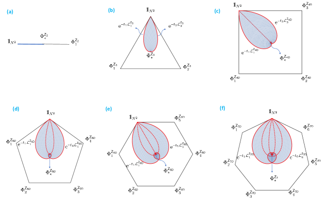
The polytope related to the group, , is the simplex of dimension one, i.e. a line segment. The set of accessible maps, in this case, can be written as (11) with probabilities given by Eq. (10)
| (16) |
Hence the trajectory starts from the identity and goes to the projector at the centre of the line at , see Fig.1(a). Thus, any map of the form with is accessible. Note that the results do not depend on the dimension of the quantum channels, and such a simplex exists in all dimensions. As an explicit example, however, one may get the qubit channel with one of the Pauli matrices.
Example 2 (The group of order ).
A group of order is still a cyclic and so an abelian group, , where the superscript denotes the cyclic group of order . Since all the members of this group are unitary channels and so the extreme points of the set of quantum channels, these channels do not lie on the same line. Thus, they are linearly independent and the polytope of the group is a triangle for -dimensional quantum channels. This triangle is regular with respect to the Hilbert-Schmidt distance between two unitary maps and ,
| (17) |
In the case of the group of order we get
| (18) |
showing all elements of the group are equidistant. Therefore, the triangle is regular for -dimensional quantum channels, and we deal with a 2-simplex. On the other hand, the order of both non-trivial elements are three, . Thus, through Eq. (13) and Eq. (14), accessible maps are given by , where and
| (19) |
These equations are already introduced in SAPZ20 in the study of
accessible Weyl channels of dimension three. The simplex representing this
group and the subset of accessible maps are shown in Fig.
1b. Since the group has no non-trivial subgroup, there is no
accessible map on the edges, as shown in this figure. Observe that this result
is independent of the dimension of the quantum channels. Again, as an explicit
example we may think of a group of three single-qubit unitary channels based on
the group up to a phase, .
Existence of a faithful representation of qubit channels for this group
guarantees the existence of a faithful representation in higher dimensions. Note
that the same non-convex subset of the equilateral triangle, plotted in Fig.
1b and bounded by two logarithmic spirals SAPZ20 , was
earlier identified in search of classical semigroups LRRL16 ; KL21 in the
space of bistochastic matrices of order three.
Concerning the spectrum, the fact that non-trivial elements are of order
implies that eigenvalues of these maps are . Perron-Frobenius theorem in the space of quantum channels
suggests all of these elements are present in the spectrum of both and . Due to the commutativity of these maps, the
spectra of channels of the form in the complex
plane are embedded in the regular triangle whose vertices are given by the
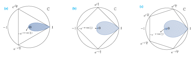
elements of the set above, see Fig. 2(a). Observe that the
spectra of accessible maps in this the triangle form the same shape bounded by
logarithmic spirals as the set of accessible maps in the simplex of
the group in the space of quantum channels – see Fig. 1(b).
Example 3 (The groups of order ).
A group of order is isomorphic either to a cyclic group or to a non-cyclic one, with and for different . Both of these groups are still abelian so one can find a set of common basis in which all the elements are diagonal. Let us first consider the cyclic group, .
III.0.1 The cyclic group of order
The polytopes of this group can be two-dimensional or three-dimensional related to the linear dependency of the elements. The spectra of the group can determine this up to a phase of Kraus operators.
Lemma 9.
Consider the cyclic group of order of quantum channels acting on -dimensional systems. Let denote its generator, i.e. for . So is the generator of a cyclic group up to a phase of order , , whose spectrum up to a general phase is from the set . Moreover, both real and imaginary elements should be present in the spectrum of to have four distinguished elements in the group . Then the elements of are linearly dependent if and only if all the real elements appearing in the spectrum of have the same sign and all the imaginary eigenvalues have also the same sign (can be different from the sign of real ones).
Proof.
For any unitary quantum channel , eigenvalues of the superoperator are determined by the eigenvalues of through . Moreover, conditions on the spectrum of imply that the eigenvalues of read . Hence in the spectra of and corresponding to each the numbers and appear, respectively. Accordingly, we get meaning that the group members are linearly dependent and the polytope of the group lies on a plane, see Fig. 1(c). On the other hand, once the condition on the spectrum of is violated, then and appear in the spectrum of . In this case, one can check that the equation implies for any , suggesting the the group elements are linearly-independent, and the polytope is then a tetrahedron. ∎
We will change the superscript as and for the linearly dependent and linearly independent case, respectively, when we need to emphasise this property. An immediate result of the above lemma is the following corollary.
Corollary 10.
For the cyclic group of order formed by qubit channels, acting on systems of dimension , elements are linearly dependent.
However, in higher dimensions both two and three dimensional polytopes are possible. In order to study the regularity of the poytope, let and denote the number of eigenvalues and , respectively, in the spectrum of , defined in Lemma 9. In a similar way let and denote the number of eigenvalues and , so that . These numbers allow us to express the Hilbert-Schmidt distance (17) between the channels,
| (20) |
The above relations imply if the polytope is of dimension , it forms a
square like the one in Fig. 1(c), while the three-dimensional case
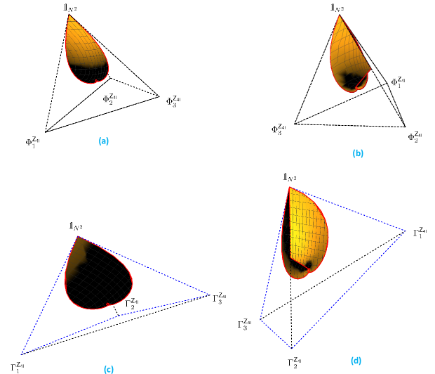
can be a (non-)regular tetrahedron – see Fig. 3. In particular, for a
cyclic group of order of linearly-independent qutrit channels one out of
four numbers and is zero due to Lemma 9, while
the remaining three numbers are equal to . This implies that both distances
in Eq. (20) are equal. Hence, the polytope is a regular tetrahedron
for a cyclic group of order, formed by linearly independent quantum channels
acting on dimensional systems. In higher dimensions, however, both regular
and non-regular tetrahedrons, as well as the square, are possible, see
Fig. 3. To emphasize the regularity of the polytope, we will denote
cyclic groups of four linearly-independent channels with a regular and
non-regular tetrahedrons by
and , respectively.
The shape of the polytope formed by the elements of the group in the space of quantum channels and the dimension of the channels do not play any role by describing the boundary of the set of accessible maps. Hence the group denotes one of three different types of the group: , , and . Due to Corollary 8, the order of the cyclic subgroups (the order of elements) plays a pivotal role. Assuming as the generator of , we get while . This implies that
| (21) |
while is the same as Eq. (16) with substitution of for , and noting that . The trajectory is the same as by replacing by and by . Hence for an accessible map of a cyclic group of order , we get with independently of the shape of its polytope and dimension of the channels. In this way we arrive at equations
| (22) |
which allow us to represent any element of the set of accessible maps as a convex combination of the group members. In the case of the group the set of accessible maps forms a non-convex subset in the square – see Fig. 1(c).
The spectra of superoperators obtained by a convex combination of the elements
of this group are also embedded in a square in the complex plane whose vertices
are . The spectra corresponding to accessible maps are
restricted to a shape equivalent to the shape of accessible maps in the set of
quantum channels, see Fig. 2(b). As a simple example for such a
group, one may think of the set of four qubit channels constructed by the group
up to a phase .
Having a qubit realization, this group can also find representations in higher
dimensions.
Fig. 3 shows the subset of accessible maps in a regular and a
non-regular tetrahedron. As mentioned in Corollary 10, it is
impossible to find such polytopes satisfying a cyclic group structure in the
space of qubit channels. Let us first consider the regular tetrahedron, Fig.
3 (a) and (b). The simplest example of a cyclic group of order four
with linearly-independent elements is a set of qutrit channels based on the
group up to a phase,
.
Due to Lemma 9 existence of both and in the spectrum of
these unitary operators implies that they are linearly independent. One can find
other examples of qutrit channels as well as channels in higher dimensions for
this group. However, the shape of accessible maps inside the tetrahedron is
independent of a particular example or even dimension of the channels.
We shall now analyze the case of a non-regular tetrahedron, presented in Fig.
3 (c) and (d). This special non-regular tetrahedron is the polytope of
a cyclic group of four linearly-independent members for which the distance of
the channels are given by
,
see Eq. (20). As it is not possible to represent such a group with
qubit and qutrit channels, we are going to analyze the set of channels acting on
-dimensional systems. A
particular example is given by a group,
,
formed according to the group up to a phase,
.
Since both and appear simultaneously in the spectrum of the generator
, the elements of this group are linearly independent, although the
elements of the group up to a phase are not linearly independent.
Recall that a cyclic group of order has one non-trivial subgroup of order . In all corresponding polytopes of this group, there exist accessible maps belonging to the line connecting the identity map to the channel corresponding to the generator of this subgroup. In tetrahedrons shown in Fig. 3 this edge of the polytope contains accessible maps, while the diagonal of the square in Fig. 1(c) also contains accessible channels. Moreover, let us emphasize that independently of the shape of the polytope representing a cyclic group of order , the spectra of superoperators corresponding to accessible channels form the same set in the complex plane as accessible maps in the square of the quantum channel itself, see Fig. 2 (b).
III.0.2 The non-cyclic group of order
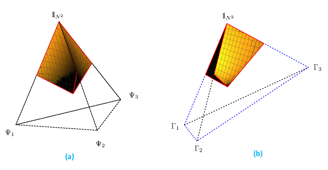
As mentioned above the non-cyclic group of order four is abelian. Due to the fundamental theorem of abelian groups, it can be obtained by the product of two cyclic groups of order whose elements are compatible with each other. Since all non-trivial group members are of order , their spectrum consists of . There exist distinguished elements of the group if there are subspaces in which the eigenvalues of all channels are not of the same sign. As for these non-trivial elements, relation holds; the negative eigenvalue should appear in the spectrum of two maps simultaneously in the same subspace, so the third channel possesses a positive eigenvalue. Taking into account all possibilities, one can prove that to have the only possibility is for any . This means the elements of are linearly independent. Thus the polytope for this group, regardless of the dimension of the channels, is a tetrahedron, see Fig. 4. Moreover, one needs to study the distance of the channels to find whether this tetrahedron is regular or not. In this case, the Hilbert-Schmidt distance (17) for different maps are given by
| (23) |
As mentioned in Example 1, the number of negative eigenvalues in a
unitary channel of order is for an . In
particular, for qubit and qutrit channels, the numbers of negative eigenvalues
can be and , respectively. This means unitary qubit channels of order
are traceless and for any unitary qutrit channels of this order, the trace of
all such channels is equal to . Thus for qubit and qutrit channels, the
tetrahedron spanned by the elements of the group is regular – see
Fig. 4 (a) and (b).
The group of Pauli channels is the well-known example of a non-cyclic group of
order whose accessibility has been studied in DZP18 ; PRZ19 . As an
example of qutrit channels forming such a group, consider three different
quantum channels gained by different permutations of the unitary operator,
. In higher dimensions, the tetrahedron can be non-regular, and
to emphasize this fact, the channels will be denoted as
, but the group does not
contain the superscript . An example of a regular tetrahedron
spanned by channels in dimension we can take identity and three unitary
operations obtained by three different permutations of
corresponding to three different quantum channels. To get a non-regular
tetrahedron consider a group up to a phase,
where , , , and
. This tetrahedron is similar to the non-regular
tetrahedron of Example 3, in which the length of two non-connected edges are
times the length of the other edges.
Note that the property of accessibility of a channel is independent of the dimension and the form of the polytope, as it depends on the group structure. In the case of a non-cyclic group of order four all non-trivial elements are of order , so individual trajectories, with only a single non-zero interaction time, are of the form (16). For an accessible map, , with we get
| (24) |
These results have already been reported for the Pauli channels DZP18 ; PRZ19 ; SAPZ20 . However, here we see that they can be gained for any set of quantum channels admitting the same group structure. The subset of accessible maps in the regular and non-regular tetrahedrons are presented in Fig. 4. Note that a non-cyclic group of order has three non-trivial subgroups, each of which is of order . Consequently, we see on the edges connecting the identity map to other three elements, accessible maps can be found.
IV Geometric properties of the set of accessible maps
In this section, we will study the geometric properties of the set of accessible maps, which are obtained by a mixture of unitary maps forming a discrete group. Proposition 1 implies that any Lindblad operator determined by a quantum channel, , generates a trajectory in the set of quantum channels which converges to the projector onto the invariant subspace of the channel . For any quantum channel , the line connecting the identity with is a tangent line to the trajectory generated by at the beginning of the evolution. To see this, note that for the dynamical semigroup , one gets
| (25) |
which proves the claim that defines the tangent line for the evolution at . Analyzing a finite group of quantum channels and the semigroup formed by convex combinations of elements of this group, a distinguished trajectory joins the identity with the centre of the polytope, which follows the direction determined by the tangent line at the beginning of evolution. Stated in other words, we have the following result.
Proposition 11.
Let define a finite group of quantum channels. The line connecting identity to the centre of the polytope, , always belongs to the set of accessible channels in this group.
Proof.
To show this we will start with the Lindbladian . Note that in this definition we ignored the trivial generator to follow the convention adopted here. So is not equal to , but . However, they generate the same dynamics up to a rescaling of time.
| (26) |
where we called the resultant channel for future reference. Furthermore, in the first equation of the second line, we used the fact that is a projector; see Proposition 6. Eq. (26) shows the line connecting the identity to the centre of polytope always belongs to the set of accessible maps and completes the proof. ∎
The above proposition leads us to the following important result.
Theorem 12.
The set of accessible maps occupies a positive measure in the polytope formed by the convex hull of the corresponding group elements.
Proof.
To prove, we will show that for any non-ending point in the interval connecting identity to the centre of the polytope, one can always find a ball that belongs to the set of accessible maps. According to above proposition, any such non-ending point can be defined as for time such that there exists with . Now let we have and . So we can define a family of valid -dependent Lindbladians as . Hence, for any satisfying above conditions belongs to the set of accessible maps at each moment of time. Thus, for we get
| (27) |
where and for . In writing these equations, we considered only the first order of and and also ignored their products. Moreover, one may notice that and consequently commute with any channel in the polytope of the group as stated in Proposition 6. The left-hand side of Eq. (27) belongs to the set of accessible maps of the group , so does a neighbourhood of any for a finite in any direction. This completes the proof. ∎
The above result was intuitive because the trajectory generated by Lindbladian corresponding to any quantum channel starts in the tangent plane of the line connecting the identity element to the assumed channel. So the set of accessible maps inside a polytope is defined by trajectories that go in all possible directions at the beginning. However, we will generalize the above approach concerning the point in the sequel to show for an abelian group at a finite time for any point on the trajectory generated by a Lindbladian corresponding to a channel from the interior of the polytope such a ball exists. Before proceeding with such an extension, let us conclude the discussion on the volume by explicit calculation of the volume for the examples mentioned in the previous section.
Proposition 13.
The ratio of the volume of the set of accessible maps to the volume of the corresponding polytope for the examples discussed in Section III reads:
-
a)
For any choice of a cyclic group of order with exactly three linearly independent elements corresponding to a regular -polygon in the plane, see Fig. 1, the ratio is given by
(28) -
b)
For a cyclic group of order with all linearly independent elements, for both regular and non-regular tetrahedrons, see Fig. 3, the ratio is given by
(29) -
c)
For the non-cyclic group of order the ratio is given by
(30) independently of the regularity of tetrahedron, see Fig. 4.
The proof of this proposition is provided in Appendix A. Note that Eqs. (28) and (30) were already presented in SAPZ20 for the ratio of the spectra of accessible to the entire set of Weyl maps and for accessible Pauli channels, respectively. However, we should emphasize that these results are valid for any representation of the aforementioned groups independently of the dimension of the maps. In Remark 19 we show that for the specific example of Weyl channels, the volume of the set of accessible and Markovian Weyl channels are the same. Accordingly, in this case, the set of the accessible maps forms a good approximation of the set of Markovian channels. Now we will apply the same approach of Theorem 12 to get the boundaries of the set assigned to an abelian group.
Theorem 14.
The boundary of the set of accessible channels in the polytope of a finite abelian group of unitary maps is formed by Lindblad operators , where belongs to the boundaries of the polytope.
Proof.
Let denote the Lindblad generator such that the channels along with identity form a group of order and for all . Then it is always possible to find a probability for small enough such that . Similar to the proof of the previous theorem, we can define a family of valid -dependent Lindblad generators . So for any finite time there is such that and belongs to the set of accessible maps. On the other hand, we have
| (31) |
where , for , and is the time-dependent probability by which the trajectory of is defined, see Theorem 4. Note that due to rearrangement theorem for any fixed the term produces all group elements with different order according to the group multiplication table. Thus we can define the -dimensional vector by its element, which can be gained by
| (32) |
where is the regular representation of element of the group of dimension defined based on the group multiplication table see Lemma 5. Therefore, one can claim the vector can define a ball around the point if the -dimensional matrix is invertible. To show that we use Lemma 5 that leads to
| (33) |
This is an invertible matrix as long as is finite, which is the case here, completing the proof. ∎
We should notice that the inverse of the theorem is not
necessarily valid, i.e. not any point from the boundaries of a polytope
formed by a finite abelian group of quantum channels can give a
trajectory at the boundaries of the set of accessible maps.
For a counterexample, see all the red dashed lines in
Fig. 1c-f. These are trajectories generated by
single Lindbladians corresponding to the channels at different
vertices of the polygons.
Our conjecture is that the inverse is true when the elements are
linearly-independent.
To proceed with investigating more geometrical properties of accessible maps, in what follows, we show that this set is star-shaped with respect to the centre of its corresponding polytope. First, note that due to Proposition 11, the line segment is accessible by the generator that commutes with all channels in the polytope. Applying this fact, we get that for any accessible
| (34) |
and therefore, the line segment is accessible, proving the following result.
Theorem 15.
The set of accessible maps in a polytope formed by a discrete finite group of quantum channels is star-shaped with respect to the centre of the polytope.
Corollary 16.
If a set of accessible maps is planar, then accessible maps are star-shaped with respect to the whole interval .
Proof.
This follows from the fact, that for any accessible , the set
| (35) |
is accessible. Next using the fact, that this is a subset of a plane, we have for all , it contains intervals of a form
| (36) |
Which shows the star shapeness with respect to the interval . ∎
V Accessibility rank, Pauli and Weyl channels
In this Section, we explicitly study some further examples of quantum channels forming a group and discuss the rank of accessible channels.
Example 4.
Let with denote eigenvalues of a superoperator corresponding to a unitary . If , where is a irreducible fraction of a rational number, then can generate a discrete and finite cyclic group of order equal to the lowest common multiple of , denoted by , i.e. .
As an example of such a group, one may consider a group of rotations around a fixed axis with discrete angles. Let us focus on qubit channels. In this case a rotation around of magnitude is gained by applying . Let us take to be one of the following angles with . It is easy to check that is an abelian group up to a phase of order . Thus is an abelian (more precisely a cyclic) group of the same order. Moreover, for every divisor of (), has at most one cyclic subgroup of order generated by different powers of . Therefore, one can always find an accessible map of order which has a convex expansion in terms of the subgroup members . The space of such a group is an -polygon. For the , the set of channels and their corresponding accessible maps are given in Fig. 1.
Example 5 (Group of commutative quantum maps forming an orthogonal basis).
An abelian group of unitary quantum maps forming an orthogonal basis, , is one of the simplest non-trivial examples to investigate. Let denote an abelian group up to a phase of such unitary matrices. Weyl unitary matrices W27 provide an example of such a set. Since we are dealing with an abelian group here, Corollary 8 clarifies the problem of accessibility. Since unitary matrices form an orthogonal basis in the Hilbert-Schmidt space of matrices and thus are linearly independent, the analyzed polytope forms a simplex in dimension . This implies that the convex combinations we get through Corollary 7 or Corollary 8 for the accessible maps are unique. Therefore, we can call the number of vertices appearing in such a unique convex combination the rank of the channel (and it equals to the Choi rank as well since the vertices are orthogonal maps). Accordingly, an immediate result of Corollary 8 is that not all quantum maps with any assumed rank can be accessible.
Proposition 17.
The set of accessible quantum maps of the form , in which ’s are unitary channels belong to an abelian group and satisfy , is formed by the maps of (Choi) rank equal to the order of possible cyclic subgroups of or their multiplications.
Through the fundamental theorem of abelian groups this the theorem can be
rephrased as follows. The set of accessible channels satisfying the above
conditions is formed by the maps of Choi rank equal to the order of possible
subgroups of . Note that through Corollary 8
it is possible not only to indicate the rank of accessible maps but also to find
which participated in the combination when an assumed is not
zero. In summary, we should expand convexly an assumed quantum channel in
terms of extreme points . Such an expansion is unique here. If the
extreme points participating in this expansion do not form a subgroup of
, then the map is not accessible.
As an example let us consider Weyl channels more explicitly.
Weyl channels are a unitary generalization of Pauli maps.
These channels are based on unitary operators of the form for
where and
with
.
The accessibility in this set is already studied in SAPZ20 .
In the case of Pauli channels is of order .
There are three different cyclic subgroups of order ,
for multiplication
of any two of them exhausts the group .
Moreover, the identity element itself is always the only trivial cyclic subgroup of
order . Therefore, there are:
(i) The identity map as the only accessible map of rank .
(ii) Accessible maps of rank two in the form of
for which are
gained when the only non-vanishing interaction time is .
(iii) The full-rank accessible maps, which are available when there are at least
two different . Fig. 4(a) presents the accessible
maps among all Pauli channels.
In the case of qutrit Weyl maps, is of order . There are four
different cyclic subgroups of order , . Again, the multiplication of any two subgroups makes the group
. In addition, there is not any other nontrivial subgroup for .
Therefore, the accessible maps belong to one of the following sets: (i) The
identity map as the only rank one accessible map. (ii)Accessible maps of rank
which can be found on the face of the simplex specified by
when or and all other interaction times are zero.
Fig. 1(b) can be considered as a cross section presenting such a
subgroup. (iii)The full-rank accessible maps which are available when there are
at least two different and where .
The above results concerning the Weyl channels are mentioned in SAPZ20 . However, the group properties of Weyl channels help us to generalize these results to a general case of -dimension. Any group of Weyl unitary maps acting on -dimensional systems, formed by cyclic subgroups of order with no element in common but the identity. This implies that the direct product of any two of them forms the group entirely. So we get
Corollary 18.
In the case of Weyl quantum maps acting on -level systems, there always exist accessible maps of rank , and . When is prime, these are the only choices, however, for a composite other ranks are possible too. The ranks correspond to the cardinality of the subgroups.
Before proceeding with the following example concerning local channels, let us mention the following simple and yet significant remark about accessible Weyl channels.
Remark 19.
The accessible Weyl channels can recover the full measure of Markovian Weyl channels but not the entire set.
The supporting evidence for this statement comes from the fact that the necessary and sufficient condition for accessibility of Weyl channels introduced in SAPZ20 is the same as the necessary and sufficient condition stated in WECC08 for Markovianity of channels with non-negative eigenvalues. Note that in the case of channels with negative eigenvalue, Markovianity can only be defined for the maps whose negative eigenvalues are even-fold degenerated DZP18 . Such a set is by definition of measure zero.
Example 6 (Tensor product of quantum channels).
Let us now generalize our results to channels acting locally in higher dimension.
Note that the set is an
abelian group up to a phase if and
are.
Moreover, it contains a complete set of orthogonal
matrices, i.e. , provided that and
are two sets of orthogonal basis in the space of matrices of order and , respectively.
Let denote the group formed by .
We will also assume that and are the sets
of orthogonal basis and are abelian up to a phase.
Therefore, the subgroups of are of
order where and are
the cardinalities of the subgroups of
and
, respectively,
and each of which is a group of orthogonal quantum maps.
In a very particular case, when we restrict ourselves to being the group related to Pauli channels, we get as the rank of an accessible map of the form acting on a two-qubit system. It is easy to generalize this result to the system of qubits, each of them is subjected to an evolution described by a Pauli map.
Corollary 20.
Let define the group obtained by a tensor product of Pauli channels. Hence each element is a map acting on a -qubit system. Then channels accessible by Pauli semigroups can only be of rank equal to with .
VI Classical stochastic maps
Any stochastic matrix describes a Markov chain – a transition in space of -point probability distributions, . By construction, each colum on forms an -point probability vector itself. Return now back to the space of density matrices. The process of decoherence transforms a quantum state into a classical probability vector embedded in its diagonal entries, , where denotes the decoherence channel. Similarly, a transition matrix can be obtained from a quantum channel suffering the super-decoherence KCPZ18 ,
| (37) |
This effect can be considered as a decoherence applied to the Choi matrix , where with denotes the maximally entangled state. Hence the classical transition matrix arises from reshaping of the diagonal entries of into a square matrix of size . Super decoherence of a quantum channel can also be described by sandwiching it between repeated action of the decoherence channel,
| (38) |
If denotes the set of Kraus operators of the channel , then is given by Hadamard product, . Thus super-decoherence transforms a unitary quantum channel, , into a unistochastic transition matrix, . Moreover, one can apply the special ordering of Gell-Mann basis where , ’s for are the diagonal elements, and for denote other elements. In that case, we can divide the distortion matrix of size defined in (2) into four blocks and the translation vector into two parts,
| (39) |
where and are square matrices of order and , respectively, and , are vectors with the same respective length. Off-diagonal blocks and are rectangular so that the dimension of is . Thus, Eq. (38) implies that the process of super-decoherence in the above basis results in a projection into a -dimensional space Ketal20 ,
| (40) |
It is worth mentioning that super-decoherence sends Lindblad generators to the set of Kolmogorov operators, i.e. the generators of classical Markovian evolutions. This fact can be observed through the GKLS form (1). The Kolmogorov generators , also called ‘transition rate matrices’, satisfy conditions: (a) for all , and (b) for all .
Lemma 21.
Proof.
If the above condition for a quantum channel holds, then the cyclic group
generated by different powers of this channel has its classical counterpart of
the same order, such that each element finds its respective element in the
classical set through super-decoherence.
A trivial example of quantum channels satisfying Lemma 21 are those for which and . This implies
| (41) |
The set of quantum channels satisfying above equation are known as Maximally
Incoherent Operation (MIO) in the context of resource theory of quantum
coherence BCP14 . This is the largest set of operations which are not able
to generate coherence in an incoherent state. So taking classical probabilities
embedded in diagonal entries of an incoherent state , the set MIO can be
seen as classical operations. Note that the super-decoherence map from quantum
channels to stochastic matrices is a surjective and non-injective function.
However, we can always find a maximally incoherent operation which is sent to
any assumed classical transition through super-decoherence. Moreover, it is
worth mentioning if satisfies Eq. (41), then the corresponding
Lindblad generator also satisfies the same condition. Such a generator can be
thus called an incoherent generator. Interestingly, for any Kolmogorov
generator one can always find an incoherent Lindblad generator
KL21 whose trajectory is an incoherent quantum channel at each moment of
time.
In the classical case, defines a group if are permutation
matrices, i.e. the extreme points of Birkhoff polytope. So the group is of
order and an arbitrary convex combination is the most general bistochastic
matrix. We assign to each element of the Kolmogorov generator . As any classical transition matrix is equivalent to an MIO,
and its Kolmogorov operator is equivalent to an incoherent Lindblad generator,
all the results of Section II are also valid for classical
transitions. However, we arrive at the same conclusion noting that the
aforementioned results are obtained by adopting the group properties and not the
fact that is a quantum channel. Hence this approach can be applied to
analyze the accessibility of classical bistochastic matrices by classical
dynamical semigroups generated by a Kolmogorov generator.
Based on the results of these work, one can easily show that a classical
dynamical semigroup is a convex combination of the group members
. If we take the cyclic permutations as the assumed group, since cyclic
permutations are orthogonal and thus linearly independent, the classical
bistochastic matrices gained by their convex combination enjoy the following
property. The set of accessible circulant bistochastic
matrices is formed by the matrices of rank equal to the order of possible
cyclic subgroups of or their multiplications.
The most general finite group in the classical domain is the set of all permutations forming the Birkhoff polytope . The first nontrivial case, which forms a non-abelian group, is the permutation group . The permutation matrices and their convex combinations make the Birkhoff polytope . This is a -dimensional set comprising the convex combination of two equilateral triangles in two orthogonal planes. To demonstrate an exemplary application of our approach, we discuss the set of accessible bistochastic matrices of order three, initially analyzed in SZ18 . The accessible set is found by exponentiating different Lindblad generators formed by subtracting the identity from a map picked from the Birkhoff polytope . The set of accessible classical channels remains in . We demonstrate this set in Fig. 5 by producing a million such accessible channels and projecting them on the orthogonal equilateral triangles.
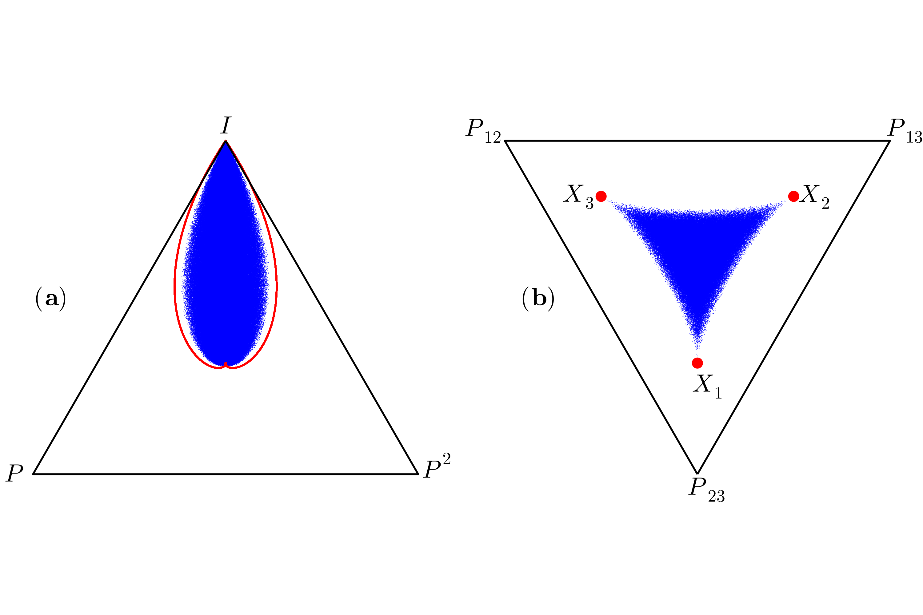
Note that the triangle with even permutations on its corners forms the convex
hull of the cyclic group of order . Therefore we expect the projection of the
accessible maps inside the to at least cover the interior of the
red curve – see Fig. 5 (a).
The data suggest that there are
no accessible maps whose projections fall outisde this curve. The case
for the odd subspace is different as there are no accessible channels that lie
on the odd subspace other than the centre of the polytope. This is true because
the spectrum of a matrix
comprises of the values
and unity. Since a positive determinant is necessary for accessibility,
we find that any combination except for is not
accessible.
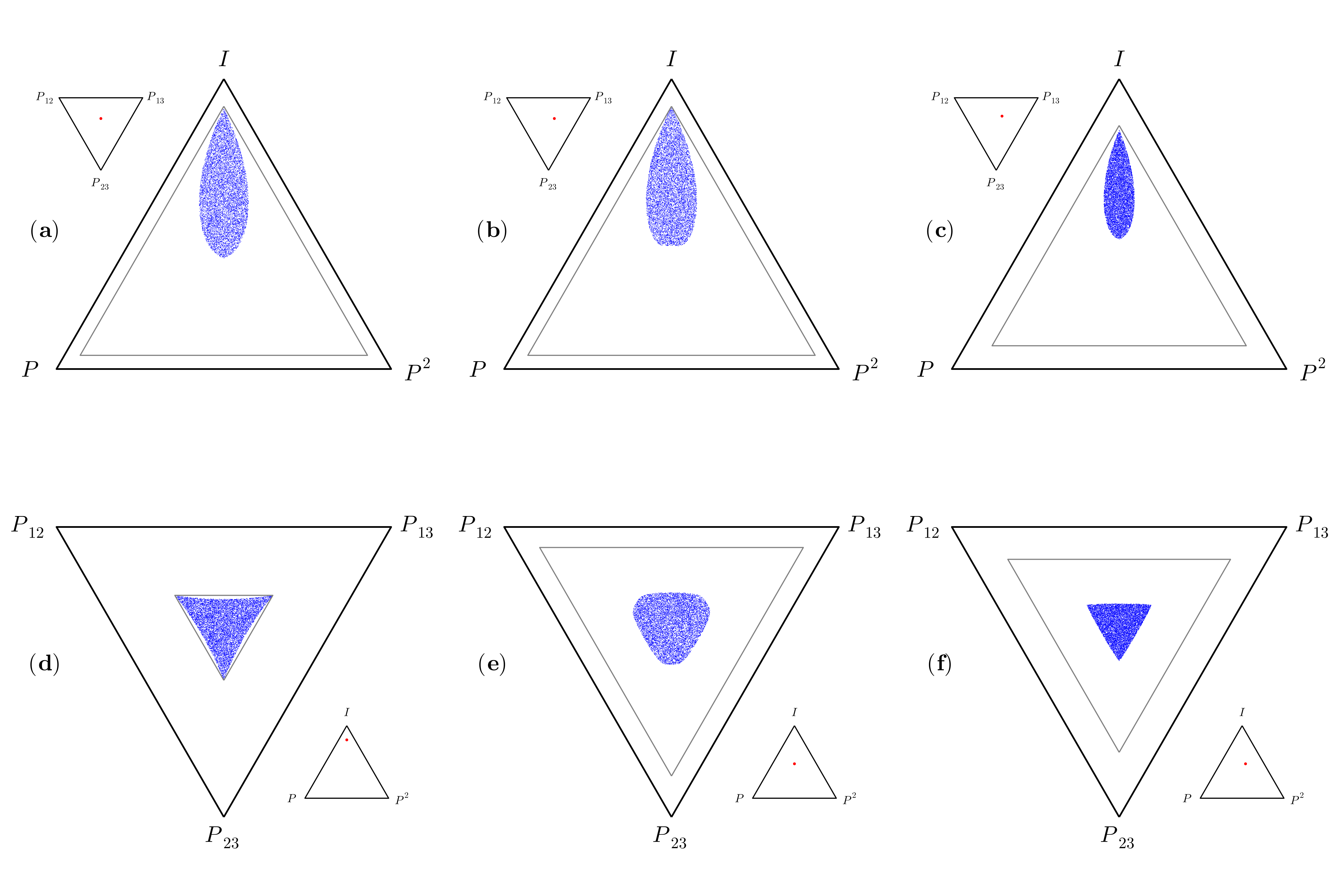
Another way to visualize the accessible matrices is to draw cross-sections with 2D planes parallel to the even or odd subspace with different displacement vectors in the orthogonal subspace. Fig. 6 includes some of these cross-sections.
The volume of the Birkhoff polytope for is known to be 9/8 BEKTZ05 . Using a Monte Carlo sampling method based on a sample consisting of points that were uniformly distributed in the Birkhoff Polytope , we estimated the relative volume of the set of accessible maps as
| (42) |
In order to decide if a particular bistochastic map was accessible or not, we
computed the matrix logarithm and checked if it was possible to write it as a
positive combination of the five generators in the form .
VII Concluding Remarks
The problem of characterization of Markovian quantum channels has attracted
considerable attention in recent years WECC08 ; SCh17 ; Si21 .
The simplest case of single-qubit maps is already well-understood
DZP18 ; PRZ19 ; CC19 ; JSP20 , while the general problem, in quantum and classical
setup, remains open.
Following SAPZ20 we analyzed in this work the set of
accessible quantum channels obtained by a Lindblad generator of the form,
, for some selected maps and
probabilities . This set forms a subset of the set of Markovian channels of
a positive volume. Instead of analyzing the structure of for a fixed
dimension of the system and a concrete choice of the maps , we
studied the case in which the maps belong to a particular group .
The key result in this work consists in identifying properties of the set of accessible maps which do not depend on the dimensionality of the
system but are determined by the properties of the group . We demonstrated
that this set has a positive volume and the star-shape property with respect to
the uniform mixture of all the maps forming the group. We computed the
volume of the set of accessible maps and analyzed its structure for several
groups – see Fig. 1 showing set for linearly dependent
channels forming cyclic groups of order and Fig. 3(b) obtained for
cyclic groups of order of linearly independent channels.
It is worth mentioning that some of the results presented here are obtained only
based on a group’s closure property. Thus, they also hold once the set of
extremal channels is a semigroup. In this way, we can also generalize the
results to the nonunital channels. For example consider the set
of qubit channels where
is the identity map, for are Pauli channels,
the nonunital maps and are completely contractive channels
into the states and , respectively. This set is a
semigroup formed by six extreme channels. Hence, their convex hull has six
vertices. However, the elements are not all linearly independent. They satisfy
. In this case, the set of accessible
maps is still confined in the convex hull of the semigroup. There are, however,
some results that need other group properties. For example, note that the
trajectory does not necessarily end in the
centre of the polytope. A counterexample happens when all probabilities
are equal to zero but . In this case, the trajectory will end in the vertex
assigned to .
Furthermore, we showed that when the vertices of the convex hull of the channels are linearly independent, the set of accessible channels contains quantum channels with (convexity) ranks satisfying certain constraints. The figures mentioned above illustrate the following three facts:
(i) In the simplest case of , accessible maps are of ranks one and two.
(ii) In the case of , the group of order , has only two trivial subgroups; identity and the group itself. Hence there exists an accessible map of rank , the identity map, and of rank . There is no accessible map of rank two, which correspond to the edges of the triangle.
(iii) For , the group has (at least) a subgroup of order two. Thus, when we have a tetrahedron, the set consists of maps of (convexity) rank (the identity map), rank on the edges assigned to the maps generating the subgroup and maps of full rank . Note that there are no maps of rank three corresponding to the faces of the tetrahedrons shown in Fig. 3 and Fig. 4.
We have also established more general results concerning ranks of accessible maps acting on larger systems.
(iv) For quantum Weyl maps acting on -level systems, the set contains maps of rank , and . If is prime, this list is complete.
(v) For a group of Pauli channels acting on a -qubit system the set contains maps of rank with .
Our approach can also be applied to the classical case. We also discussed when classical and quantum accessible maps could be compared directly. The present study leaves several questions open. Let us list here some of them.
-
1.
Characterize the set of points such that the set has the star-shape property with respect to them.
-
2.
Find a criterion allowing one to decide whether a given channel is accessible with respect to a given set of quantum maps .
-
3.
What is the relative measure of the set of accessible channels with respect to Markovian channels?
Acknowledgements.
It is a pleasure to thank Seyed Javad Akhtarshenas, Dariusz Chruściński and Kamil Korzekwa for inspiring discussions and helpful remarks and David Amaro Alcalá for useful correspondence. Financial support by Narodowe Centrum Nauki under the Maestro grant number DEC-2015/18/A/ST2/00274 and by Foundation for Polish Science under the Team-Net project no. POIR.04.04.00-00-17C1/18-00 are gratefully acknowledged.Appendix A The Group Matrix/Table; Proof of Proposition 13
In this Appendix, we try to calculate the accessibility volume fraction for some
abelian groups thereby providing proof for the results presented in
Proposition 13.
The volume measure is induced from the Euclidean metric on the dynamical maps (see (2)). For unitary channels, or a mixture of unitary channels, the vector is zero, and we need only consider the affine matrix . In fact, the affine matrices themselves form a representation of our group of interest. Furthermore, for abelian groups, we may work in a basis in which all the affine matrices are diagonal, thereby making all the convex mixtures diagonal as well. Finally, since we are only dealing with diagonal matrices, it sounds reasonable to write down the diagonal entries of each affine matrix in the group in columns of a table. The table will therefore form a matrix with rows (remember that the affine matrices are of order where is the dimension of the Hilbert space.) and columns. For example, a possible group table for a qubit representation of the non-cyclic group with four members () is the following matrix
| (43) |
In general the table looks like below
| (44) |
where denotes an dimensional column vector with all its components being equal to unity and the height of the table is given by . Note that changing the values of (and therefore ) changes the shape and size of the tetrahedron; however, as we will see, the accessibility volume fraction will remain invariant as long as the parameters all remain positive. Part (c) of Proposition 13 can now be restated as regardless of the values for the group , the accessible channels cover a fraction of the corresponding tetrahedron’s volume.
Proof.
Let be the origin of the coordinate system and define the vectors
| (45) |
Then the tetrahedron consists of the diagonal matrices with the constraints
| (46) |
The line-element is with the metric
| (47) |
Therefore the volume of the tetrahedron is given by
| (48) |
It remains to calculate the volume of the accessible channels. These are found by element-wise exponentiation of the diagonal vectors This time the only constraint is and the metric is
| (49) |
with
| (50) |
hence
| (51) |
Therefore, the volume is
| (52) |
Finally
| (53) |
∎
It is possible to repeat the same procedure for the groups to prove the
following.
Proposition 22.
The accessibility volume ratios for are given by
For 3D cyclic groups of order 4, the result is slightly different. Indeed, part (b) of Proposition 13 is now rephrased as for all values of with , the accessible channels cover a fraction of the tetrahedron’s volume.
Proof.
Let us start again with the group table.
| (54) |
Since we are working with a real vector space, it is convenient to merge the diagonal imaginary matrix
| (55) |
with the real matrix
| (56) |
The group table then becomes
| (57) |
with .
Defining as we did in the previous proof, we get the metric
| (58) |
which leads to
| (59) |
Now for the accessible channels, if we use the coordinates, we get
However, these coordinates are not injective: the periodic functions in the first part will re-address the same point many times, leading to an overestimating of the volume by evaluating the integral as before. So let us use defined as
| (60) |
The constraints become
| (61) |
Note that the angle is manually constrained to stay in the interval . The metric is
| (62) |
Therefore
| (63) |
Finally, the accessible volume is
| (64) |
∎
A unitary channel for -dimensional quantum systems has an affine map where is an dimensional rotation matrix. Dealing with Abelian subgroups allows us to diagonalize the rotation matrices simultaneously and only worry about the spectral configuration of the group members, see also section 5 of SSMZK21 .
Proposition 23.
For the 2 dimensional cyclic group , where all the members lie on a 2D plane, a fraction
| (65) |
of the 2D regular polygon is covered by exponentiating the Lindblad generators.
Proof.
Forgetting about the scale of the actual polygon, we may identify it with the complex polygon with vertices . Then the area of the polygon is
| (66) |
By exponentiating the Lindblad generators, we get the complex set
| (67) |
A standard calculation of the area of this set leads to the claimed result.
Observation: Any complex number with is infinitesimally divisible. It may be interesting to calculate for other groups as well.
∎
References
- (1) V. Gorini, A. Kossakowski, and E. C. G. Sudarshan, “Completely positive dynamical semigroups of -level systems”, J. Math. Phys. 17, 821 (1976).
- (2) G. Lindblad, “On the generators of quantum dynamical semigroups”, Commun. Math. Phys. 48, 119 (1976).
- (3) D. Chruściński and S. Pascazio, “A brief history of the GKLS Equation”, Open Syst. Inf. Dyn. 24, 1740001 (2017).
- (4) M. M. Wolf, J. Eisert, T.S. Cubitt, and J.I. Cirac, “Assessing non-Markovian dynamics”, Phys. Rev. Lett. 101, 150402 (2008).
- (5) Á. Rivas, and S. F. Huelga, Open Quantum Systems. An Introduction, (Springer, 2011).
- (6) A. Shabani, and D. A. Lidar, “Vanishing quantum discord is necessary and sufficient for completely positive maps”, Phys. Rev. Lett. 102, 100402 (2009).
- (7) A. Shabani, and D. A. Lidar, “Erratum: vanishing quantum discord is necessary and sufficient for completely positive maps [Phys. Rev. Lett. 102, 100402 (2009)]”, Phys. Rev. Lett. 116, 049901 (2016).
- (8) A. Brodutch, A. Datta, K. Modi, Á. Rivas, and C. A. Rodríguez-Rosario, “Vanishing quantum discord is not necessary for completely positive maps”, Phys. Rev. A 87, 042301 (2013).
- (9) F. Buscemi, “Complete positivity, Markovianity, and the quantum data-processing inequality, in the presence of initial system-environment correlations”, Phys. Rev. Lett. 113, 140502 (2014).
- (10) J. M. Dominy, A. Shabani, and D. A. Lidar, “A general framework for complete positivity”, Quant. Inf. Process. 15, 465 (2016).
- (11) W. F. Stinespring, “Positive functions on -algebras”, Proceedings of the American Mathematical Society 6, 211 (1955).
- (12) J. F. C. Kingman, “The imbedding problem for finite Markov chains”, Probab. Theory Relat. Fields 1, 14 (1962).
- (13) J. T. Runnenburg, “On Elfving’s problem of imbedding a time-discrete Markov chain in a time-continuous one for finitely many states”, Proc. Kon. Ned. Akad. Wet. Ser. A 65, 536 (1962).
- (14) P. Carette, “Characterizations of embeddable stochastic matrices with a negative eigenvalue”, New York J. Math 1, 129 (1995).
- (15) E. B. Davies, “Embeddable Markov matrices”, Electron. J. Probab. 15, 1474 (2010).
- (16) K. Korzekwa, and M. Lostaglio, “Quantum advantage in simulating stochastic processes”, Phys. Rev. X 11, 021019 (2021).
- (17) L. V. Denisov, “Infinitely divisible Markov mappings in quantum probability theory”, Theory Probab. Appl. 33, 392 (1989).
- (18) M. M. Wolf, and J. I. Cirac, “Dividing quantum channels”, Comm. Math. Phys. 279, 147 (2008).
- (19) T. S. Cubitt, J. Eisert, and M. M. Wolf, “The complexity of relating quantum channels to master equations”, Commun. Math. Phys. 310, 383 (2012).
- (20) D. Davalos, M. Ziman, and C. Pineda, “Divisibility of qubit channels and dynamical maps”, Quantum 3, 144 (2019).
- (21) Z. Puchała, Ł. Rudnicki, and K. Życzkowski, “Pauli semigroups and unistochastic quantum channels”, Phys. Lett. A 383, 2376 (2019).
- (22) S. Chakraborty, and D. Chruściński, “Information flow versus divisibility for qubit evolution”, Phys. Rev. A 99, 042105 (2019).
- (23) V. Jagadish, R. Srikanth, F. Petruccione, “Convex combinations of Pauli semigroups: geometry, measure and an application”, Phys. Rev. A 101, 062304 (2020).
- (24) K. Siudzińska and D. Chruściński, “Memory kernel approach to generalized Pauli channels: Markovian, semi-Markov, and beyond”, Phys. Rev. A 96, 022129 (2017).
- (25) F. Shahbeigi, D. Amaro-Alcalá, Z. Puchała, and K. Życzkowski, “Log-Convex set of Lindblad semigroups acting on -level system”, J. Math. Phys. 62, 072105 (2021).
- (26) K. Siudzińska, “Markovian semigroup from mixing non-invertible dynamical maps”, Phys. Rev. A 103, 022605 (2021).
- (27) H. Weyl, “Quantenmechanik und Gruppentheorie”, Z. Physik 46, 1 (1927).
- (28) F. Shahbeigi, K. Sadri, M. Moradi, K. Życzkowski, and V. Karimipour, “Quasi-inversion of quantum and classical channels in finite dimensions”, Journal of Physics A: Mathematical and Theoretical, 54, 34 (2021).
- (29) P. Lencastre, F. Raischel, T. Rogers and P. G. Lind, “From empirical data to time-inhomogeneous continuous Markov processes”, Phys. Rev. E 93, 032135 (2016).
- (30) K. Korzekwa, S. Czachórski, Z. Puchała, and K. Życzkowski, “Coherifying quantum channels”, New J. Phys. 20, 043028 (2018).
- (31) R. Kukulski, I. Nechita, Ł. Pawela, Z. Puchała, and K. Życzkowski, “Generating random quantum channels”, J. Math. Phys. 62, 062201 (2021).
- (32) T. Baumgratz, M. Cramer, and M. B. Plenio, “Quantifying coherence”, Phys. Rev. Lett. 113, 140401 (2014).
- (33) M. Snamina and E.J. Zak, “Dynamical semigroups in the Birkhoff polytope of order 3 as a tool for analysis of quantum channels”, preprint arXiv:1811.09506
- (34) I. Bengtsson, A. Ericsson, M. Kuś, W. Tadej, K. Życzkowski, “Birkhoff’s polytope and unistochastic matrices, N=3 and N=4”, Commun. Math. Phys., 259, 307 (2005).