Access Points in the Air: Modeling and Optimization of Fixed-Wing UAV Network

The research on UAV networks, where UAVs serve as APs, has attracting considerable attention from both academia and industry [7, 8, 9, 10, 11, 4]. The UAV trajectory optimization problem was considered in [8], where UAVs provided service to cell edge users to offload the data traffic of terrestrial cellular network. Specifically, UAV trajectory and user scheduling were alternately optimized to maximize the sum rate of UAV-served edge users with the rate constraint of all the users. In [9], a distributed UAV deployment algorithm was proposed to minimize the distance from UAV APs to GUs so as to improve the user coverage. Moreover, the UAV AP deployment problem has been extended into heterogeneous networks [10]. Especially, a latency-aware approach has been proposed, which jointly optimizes the location and association coverage of UAVs, to minimize the total average latency of GUs considering the existing terrestrial base stations (TBSs). If frequency resources are shared by UAV APs and TBSs, potential cross-layer interference will be generated, which may degrade the performance of the UAV network. The performance of a UAV integrated terrestrial cellular network is evaluated in [11, 4]. Especially, the impact of UAV deployment density on the performance of the coexisting system was captured in [11] and an effective interference avoidance scheme was proposed to mitigate the air-to-ground interference and significantly improve the spectrum efficiency of the coexisting system in [4].

Due to flexible deployment and low expenditure, rotary-wing UAVs are applied in most of the available research [7, 8, 9, 10, 11, 4], where rotary-wing UAVs were assumed to move according to the preset trajectory and steadily stay in a given position. Accordingly, rotary-wing UAV systems have been designed and developed by a number of companies and operators [12, 13]. However, since most of off-the-shelf rotary-wing UAVs are battery driven, they are energy-inefficient and excessive power is required especially when they are taking off, climbing and changing the flight attitude. Therefore, the flight endurance of the rotary-wing UAVs is significantly limited (dozens of minutes for battery-driven ones). Moreover, limited wireless backhaul will bottleneck the performance of the UAV system supposing that high data rates are required by the connected GUs. To address the issues of limited flight endurance and backhaul, AT&A was reported to develop a tethered UAV system, named Flying COW [13]. Particularly, each rotary-wing UAV, which was connected to the ground by a thin tether, is capable of providing the long-term evolution (LTE) coverage to GUs. The tether was used for conveying highly secure backhaul via fiber and supplying power, which allows for longer flight time.

Although Flying COW is designed to ultimately provide coverage to an area up to 40 square miles, the tether connection will inevitably limit the deployment and mobility of UAVs. On the other hand, researchers and engineers are increasingly focusing on the development of the fixed-wing UAVs [14, 15, 5, 16]. Compared with the rotary-wing UAVs, the deployment of fixed-wing UAVs is more flexible. For instance, fixed-wing UAVs could offer better aerodynamic performance, which makes them well suited for the application in higher flight altitude, greater payload and longer ranges and flight endurance. In [16], an all-weather fixed-wing emergency communication system was developed for the quick network recovery in the emergency communication scenarios. According to the aerodynamic principle, nevertheless, fixed-wing UAVs cannot steadily stay in a given position and have to hover in the air. If the hover radius is large, rotary-wing UAVs would fail to provide continuous service to GUs. Moreover, although sufficient backhaul can be provided through mmWave link [17, 18], the high mobility of the hovering fixed-wing UAVs may seriously deteriorate mmWave link capacity since the mmWave beam is highly directional. Worse still, the acquisition of real-time perfect channel state information (CSI) in the highly dynamic network is challenging and remains to be an open problem [19]. Especially, the acquired CSI would be easily outdated at the moment of decision due to the on-the-move feature of fixed-wing UAVs. Therefore, the performance and deployment of fixed-wing UAV network remains to be further investigated, which motivates this work.

In this paper, we model a downlink UAV network, where fixed-wing UAV APs provide service to GUs and mmWave is applied to provide wireless backhaul. In particular, the impact of key parameters, including UAV flight altitude, deployment density, hover radius, backhaul limitation and user association rules, etc., on the performance of UAV network has been evaluated. On this basis, we further investigate how to effectively improve the UAV network performance through adjusting UAV beamwidth. The main conclusions of this work are summarized as follows.

• •

  Real-time VS semi-real-time user association rules. We evaluate the performance of two typical user association rules, namely, real-time user association (RTNA), where GUs always connect the closest UAVs, and semi-real-time user association (Semi-RTNA), where GUs connect to the UAVs whose hover centers are the closest, in terms of network spatial throughput (ST). It is shown that network ST is greatly degraded by increasing the UAV hover radius under Semi-RTNA. The reason is that desired signal power is likely to be reduced if the associated UAVs hover apart under large hover radius. Worse still, the increase of hover radius would notably increase the mmWave mainlobe beamwidth, thereby reducing the mainlobe gain and backhaul capacity. On the contrary, the impact of hover radius on the performance of RTNA is shown to be minor even though more handover overhead is introduced. Especially, if ignoring the backhaul limitation, network ST is shown to be independent of the hover radius under RTNA.

• •

  Optimization of UAV beamwidth. The impact of UAV beamwidth on network ST is further investigated. Particularly, reducing the UAV beamwidth first increases (due to alleviating overlap-cell interference) and then decreases (due to limiting UAV coverage) network ST. Moreover, the optimal beamwidth is shown to be dependent on the activated UAV density $\lambda_{\mathrm{a}}$. Accordingly, we propose a projection area equivalence policy to optimize the UAV beamwidth. In particular, network ST could be sustainably increased with UAV density if UAV half-beamwidth inversely grows with $\frac{1}{\sqrt{\lambda_{\mathrm{a}}}}$. More importantly, the optimized network ST is proved to be independent of the UAV flight altitude in the backhaul-unlimited case. In other words, aerial spatial resources can be fully exploited by the proposed policy.

We organize the remaining parts of this paper as follows. System model is given in Section II followed by the performance analysis of two typical user association rules in UAV network with respect to user coverage probability and network ST in Section III. In Section IV, we further investigate the impact of UAV antenna beamwidth on the performance of directional-antenna UAV network and optimize network ST through adjusting UAV beamwidth. Finally, conclusions are drawn in Section V. The main parameter notations used in the paper are summarized in Table I.

Consider a downlink UAV network, where fixed-wing UAV APs provide service to GUs. For the two-dimension (2D) locations, UAVs and GUs are distributed as two independent homogeneous Poisson Point Processes (PPPs) $\Pi_{\mathrm{UAV}}=\left\{\mathrm{UAV}_{i}\right\}$ $\left(i\in\mathbb{N}\right)$ with density $\lambda$ and $\Pi_{\mathrm{GU}}=\left\{\mathrm{GU}_{j}\right\}$ $\left(j\in\mathbb{N}\right)$ with density $\lambda_{\mathrm{GU}}$, respectively. For practical concern, we assume that fixed-wing UAVs hover in the air with identical hover radius $R_{\mathrm{h}}$ and different flight altitude $h_{\mathrm{UAV}}$, which follows uniform distribution $h_{\mathrm{UAV}}\sim\mathcal{U}\left(h_{\mathrm{L}},h_{\mathrm{U}}\right)$. Supposing that GUs are of identical height $h_{\mathrm{GU}}$, the vertical distance $\Delta h\left(=h_{\mathrm{UAV}}-h_{\mathrm{GU}}\right)$ from UAVs to GUs follows uniform distribution $\Delta h\sim\mathcal{U}\left(\tilde{h}_{\mathrm{L}},\tilde{h}_{\mathrm{U}}\right)$, where $\tilde{h}_{\mathrm{L}}=h_{\mathrm{L}}-h_{\mathrm{GU}}$ and $\tilde{h}_{\mathrm{U}}=h_{\mathrm{U}}-h_{\mathrm{GU}}$. It is assumed that multiple GUs can simultaneously connect to one UAV AP for service. For scheduling fairness, each UAV AP randomly and independently serves the connected GUs in a time-division manner. Therefore, the GUs in one UAV cell have the equal chance to be served. To improve frequency reuse, spectrum is reused by different UAV cells. As a result, the neighboring UAV APs may potentially generate inter-cell interference to the intended GU. If not properly handled, the inter-cell interference may significantly degrade the performance of the downlink UAV network. Besides, saturated data model is adopted such that each GU always has data request from the connected UAVs.

We adopt the following two user association rules to balance the UAV coverage performance and handover overhead.

• •

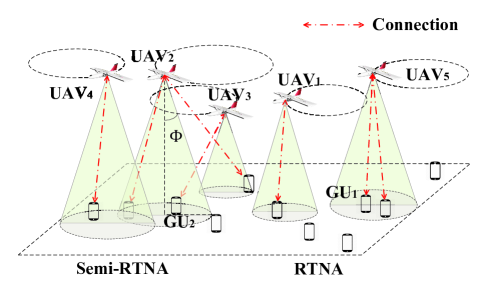
  Real-time nearest association (RTNA). One GU is associated with the UAV, which is horizontally closest to the GU¹¹1The flight altitude of UAV APs may be varying due to air buoyancy and attitude control to ensure that the hovering UAVs could cover a given area. Therefore, each GU is assumed to connect to horizontally closest UAV for stronger average received power and better coverage.. It is shown in Fig. 1 that $\mathrm{GU}_{1}$ is located closer to the hover center of $\mathrm{UAV}_{1}$ compared to that of $\mathrm{UAV}_{5}$. However, the hovering $\mathrm{UAV}_{5}$ is closer to $\mathrm{GU}_{1}$ in the current time slot. Therefore, $\mathrm{GU}_{1}$ is associated with $\mathrm{UAV}_{5}$ under RTNA. In the coming time slots, when $\mathrm{UAV}_{1}$ hovers closer, $\mathrm{GU}_{1}$ will be handover to $\mathrm{UAV}_{1}$.

• •

  Semi-real-time nearest association (Semi-RTNA). One GU is associated with the UAV, the hover center of which is horizontally closest to the GU. It is shown in Fig. 1 that, even if $\mathrm{GU}_{2}$ is closer to $\mathrm{UAV}_{2}$ in the current time slot, $\mathrm{GU}_{2}$ is associated with $\mathrm{UAV}_{3}$ under Semi-RTNA to reduce the handover overhead.

It is assumed that real-time location information of UAVs could be acquired by GUs for performing RTNA and Semi-RTNA. Accordingly, GUs could calculate the distance to the UAVs, which could provide coverage, to determine the UAV to connect to. Then, the handover of user association is initiated by the GU, which sends the handover request to the associated UAV AP and the UAV AP to connect to. Note that the handover frequency is dependent on the location of GUs, number of fixed-wing UAV APs near the GUs, hover radius and velocity of UAV APs. If not properly handled, the frequent handover will result in considerable handover overhead, thereby degrading the performance of the UAV network.

It is shown in Fig. 1 that each UAV with constant transmit power $P$ is equipped with one directional antenna. The azimuth and elevation beamwidths are $2\Phi$ with $\Phi\in\left(0,\frac{\pi}{2}\right)$. Denoting $\phi$ and $\varphi$ as the azimuth and elevation angles, respectively, the antenna gain in the direction $\left(\phi,\varphi\right)$ (corresponding to the antenna mainlobe) is modeled as [20]

where $G_{0}=2.2846$. Accordingly, the projection of each UAV on the ground is a disk region with radius $R_{\mathrm{p}}=\Delta h\tan\Phi$. If one GU is out of the projection area of any UAV, no service will be provided. Note that, although increasing $\Phi$ could enhance the UAV coverage, it will result in greater overlap of the projection areas, which may introduce excessive inter-cell interference.

The channel from UAVs to GUs is assumed to consist of pathloss $d^{-\alpha}$ and Rayleigh fading $h\sim\mathcal{CN}\left(0,1\right)$ [21, 22], where $d$ and $\alpha$ denote the distance from one UAV to its associated GU and pathloss exponent, respectively.

We consider that mmWave is used to convey wireless backhaul for fixed-wing UAVs owing to 1) higher frequency bands, which is non-overlapping with those in UAV-GU channel, and 2) greater bandwidth and backhaul capacity [6, 23]. For instance, it was tested in [24] that approximately 10Gbps transmission rate with <20% outage could be provided through 200m mmWave transmissions over Ka band (28GHz), V band (60GHz) and E band (73GHz) even if 3 blockages exist between mmWave transmitters and receivers. Since the number of ground gateways is limited, we assume that mmWave backhaul capacity is shared by the UAVs within the region of radius $R_{\mathrm{m}}$ [23, 25, 26]. Specifically, each UAV occupies equal proportion of backhaul resources. According to [25, 26], the backhaul capacity for each UAV is given by

where $C_{\mathrm{t}}$ denotes the normalized backhaul capacity in $\mathrm{bits}/\left(\mathrm{s\cdot Hz}\right)$ and $\lambda_{\mathrm{a}}$ denotes the density of activated UAVs²²2Note that UAVs would keep inactivated with no backhaul requirement if no GUs are connected.. Therefore, the denominator $\lambda_{\mathrm{a}}\pi R_{\mathrm{m}}^{2}$ denotes the number of activated UAVs within the region.

In (2), $G_{\mathrm{m}}\left(\vartheta\right)=\frac{2\pi}{\vartheta}$ denotes the mmWave mainlobe gain and $F_{\left|\varepsilon\right|}\left(\vartheta\right)$ denotes the mmWave orientation effective function [23], which is dependent on mmWave mainlobe beamwidth $\vartheta$ and orientation error $\varepsilon$. Given $\left|\varepsilon\right|\leq\frac{\vartheta}{2}$, backhaul could be effectively conveyed through mmWave. Otherwise, UAV fails to obtain backhaul due to the orientation error. Supposing that the mmWave mainlobe could cover the UAV hover region, we have $\vartheta=2\arctan\left(\frac{R_{\mathrm{h}}}{h_{\mathrm{UAV}}}\right)$ under large $h_{\mathrm{UAV}}$. Accordingly, increasing the UAV hover radius may alleviate the impact of orientation error, while reduces the mmWave mainlobe gain.

In this work, we use coverage probability (CP) and network ST to evaluate the performance of the UAV network. In particular, one GU is in coverage when 1) the GU is in the projection area of UAVs and 2) the data transmission from the associated UAV to the GU is successful. Without loss of generality, we denote the link, which consists of $\mathrm{UAV}_{0}$ and $\mathrm{GU}_{0}$, as the typical link. Accordingly, the CP of the typical link is defined by

In (3), $E_{\mathrm{p}}$ denotes the event that $\mathrm{GU}_{0}$ is within the projection area of $\mathrm{UAV}_{0}$ and we denote the corresponding projection probability as $p_{\mathrm{p}}=\mathbb{P}\left\{\left\|\mathrm{UAV}_{0}-\mathrm{GU}_{0}\right\|<R_{\mathrm{p}}\right\}$. If $E_{\mathrm{p}}$ occurs, $\mathbb{P}\left\{\mathsf{SIR}>\tau\left|E_{\mathrm{p}}\right.\right\}$ denotes the transmission success probability, where $\mathsf{SIR}$ denotes the signal-to-interference ratio (SIR) at $\mathrm{GU}_{0}$ and $\tau$ is the SIR threshold.

Based on (3), network ST is defined by

With the constraint of $C_{\mathrm{b}}$, $\mathsf{ST}$ captures how many bits could be successfully conveyed over unit time, frequency and area by the UAV network under limited backhaul.

With Semi-RTNA, the SIR at $\mathrm{GU}_{0}$ can be expressed as

where $d_{0}$ denotes the distance from $\mathrm{UAV}_{0}$ to $\mathrm{GU}_{0}$ and $I^{\mathrm{SR}}=\underset{\tiny{\mathrm{UAV}_{i}\in\mathrm{\tilde{\Pi}_{UAV}}\backslash\mathrm{UAV}_{0}}}{\sum}PH_{\mathrm{UAV}_{i}}d_{i}^{-\alpha}$ denotes the interference stemming from other activated UAV cells. $H_{\mathrm{UAV}_{i}}$ denotes the channel power gain due to small-scale fading and $\mathrm{\tilde{\Pi}_{UAV}}$ denotes the set of activated UAVs with density $\lambda_{\mathrm{a}}=q_{\mathrm{a}}\lambda$. Due to UAV association, the UAV activation probability is given by [27]

where $\eta=\lambda/\lambda_{\mathrm{GU}}$ denotes the ratio of UAV density to GU density and $\mu$=3.5. Moreover, we suppose that the mmWave orientation error $\varepsilon$ in (2) follows exponential distribution[23, 28]. Therefore, the mmWave effective function is given by the following lemma³³3Note that the results in Lemma 1 can be feasibly extended to the cases, where other distributions are applied to model the orientation error..

Proof: Please refer to Appendix A-A.∎

On average, the mmWave effective function $F_{\left|\varepsilon\right|}\left(\vartheta\right)$ in (7) could capture the impact of mean orientation error $\bar{\varepsilon}$ and mmWave mainlobe beamwidth $\vartheta$ on the performance of mmWave transmission. Specifically, $F_{\left|\varepsilon\right|}\left(\vartheta\right)$ is shown to be reduced by either the increase of $\bar{\varepsilon}$ or the decrease of $\vartheta$, which complies with intuition. According to Lemma 1, it can be shown that $G_{\mathrm{m}}\left(\vartheta\right)F_{\left|\varepsilon\right|}\left(\vartheta\right)$ in (2) is a decreasing function of the mmWave mainlobe beamwidth $\vartheta$. Since $\vartheta=2\arctan\left(\frac{R_{\mathrm{h}}}{h_{\mathrm{UAV}}}\right)$, increasing the UAV hover radius would potentially degrade the mmWave backhaul capacity.

Aided by (5), (6) and Lemma 1, CP and network ST under Semi-RTNA could be obtained in the following proposition.

Proof: Please refer to Appendix A-B.∎

It is observed from Proposition 1 that the CP and ST of UAV APs are dependent on the flight altitude of UAVs, UAV hover radius and mmWave backhaul constraint, etc. Moreover, it is shown from (9) that the expression of CP is in complicated form, which is due to the varying flight altitude of UAVs. To shed light on the impact of hover radius on the performance of UAV network, we analyze the upper bound of CP given a fixed flight altitude in the following corollary.

Proof: Please refer to Appendix A-C.∎

Following Corollary 1, it can be shown that $\frac{\partial\hat{\mathsf{CP}}_{\pi/2\left|\Delta h\right.}^{\mathrm{SR}}}{\partial R_{\mathrm{h}}}<0$. This indicates that increasing the UAV hover radius would deteriorate the performance of UAV network under Semi-RTNA rule⁴⁴4Note that deconditioning $\Delta h$ through calculating the expectation of $\Delta h$ will not disprove the above results.. On the one hand, when the associated UAV is departing from the GU, the transmission distance will be increased, thereby reducing the desired signal power. On the other hand, when the neighboring UAVs are approaching the intended GU, inter-cell interference becomes severe and dominates the performance of air-to-ground transmission.

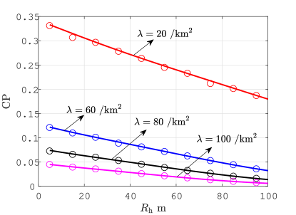
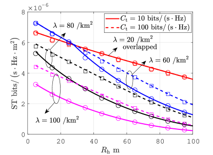
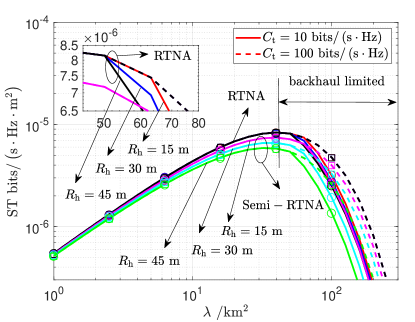
To verify the above results, we plot Fig. 2, which shows CP and network ST as a function of UAV hover radius $R_{\mathrm{h}}$ under different UAV deployment densities $\lambda$ and backhaul capacity constraints $C_{\mathrm{t}}$. It can be seen that either CP or network ST decreases with $R_{\mathrm{h}}$ under different UAV densities. In particular, network ST is more significantly degraded given smaller $C_{\mathrm{t}}$, e.g., $C_{\mathrm{t}}=10$bit/$\left(\mathrm{s}\cdot\mathrm{Hz}\right)$, and greater $\lambda$, e.g., $\lambda>60/\mathrm{km}^{2}$. As discussed, the reason is that the hovering feature of UAVs would result in the connection discontinuity of GUs. In consequence, the UAV-GU transmission is more vulnerable to air-to-ground interference especially when more UAVs are deployed. Moreover, the mmWave mainlobe beamwidth has to be adaptively increased with the UAV hovering range so as to provide sufficient backhaul, which nevertheless reduces the mmWave mainlobe gain and limits the backhaul link capacity.

If frequent handover is allowed under RTNA, the performance of UAV network could intuitively be improved since GUs always connect to the closest hovering UAVs. In this light, we analyze CP and network ST under RTNA in the following proposition.

Proof: Please refer to Appendix A-D.∎

It is shown in Proposition 2 that the CP under RTNA is independent of the UAV hover radius. This is because, when hover radius is increased or decreased, GUs could always be associated with the closest UAV. In consequence, the problem raised by the hover of UAVs in Semi-RTNA rule will be alleviated, i.e., dominant interference due to approaching neighboring UAVs and reduced desired signal power due to departing associated UAVs.

Even though the results in Proposition 2 are still in complicated forms, we make a comparison of the two rules with the aid of Corollary 1. Deconditioning $\Delta h$ in (13), we have

where (a) follows by setting $R_{\mathrm{h}}=0$ because $\hat{\mathsf{CP}}_{\pi/2\left|\Delta h\right.}^{\mathrm{SR}}$ is a decreasing function of $R_{\mathrm{h}}$. Since $\mathsf{CP}_{\pi/2}^{\mathrm{SR}}<\mathbb{E}_{\Delta h}\left[\hat{\mathsf{CP}}_{\pi/2\left|\Delta h\right.}^{\mathrm{SR}}\right]$ (see Corollary 1) and the impact of mmWave backhaul is identical to RTNA and Semi-RTNA, (16) indicates that RTNA outperforms Semi-RTNA in terms of CP and network ST.

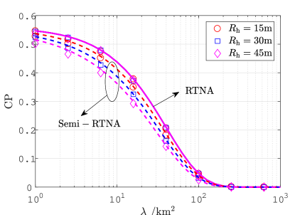
In Fig. 3, we plot CP and network ST with varying UAV deployment density $\lambda$ under Semi-RTNA and RTNA. It is shown that RTNA outperforms Semi-RTNA in terms of CP and network ST. As indicated by Proposition 2, the CP is shown to be independent of the UAV hover radius under RTNA in Fig. 3a. Moreover, when $\lambda$ is small, the network ST obtained by RTNA overlaps under different hover radii, which is shown in Fig. 3b. When $\lambda$ increases, limited wireless backhaul will be shared by more UAVs. In consequence, it can be seen in Fig. 3b that network ST is more significantly degraded (solid lines) in the backhaul-limited region. Moreover, it can be seen that a greater hover radius would lead to a more rapid decrease of network ST. As discussed earlier, the reason is that the mmWave link capacity will be decreased with the high mobility of UAVs due to reduced mainlobe gain. Consequently, the UAV network performance is more likely to be dominated by limited backhaul.

In addition, compared to the terrestrial network, in which the coverage of terrestrial APs is limited, the coverage of UAVs is greatly enhanced due to higher deployment altitude, which increases the overlapping area of the UAV cells. As a result, it is shown in Fig. 3 that network ST begins to diminish with UAV density $\lambda$ even when $\lambda$ is small, e.g., $\lambda>40/\mathrm{km}^{2}$, due to the inter-cell interference caused by overlapping UAV cells. This can be analytically verified through Proposition 2. For this reason, it is crucial to investigate how to alleviate the overwhelming interference in the UAV network, which is discussed in Section IV.

When Semi-RTNA is applied, the SIR at $\mathrm{GU}_{0}$ can be expressed as

where $G\left(\phi,\varphi\right)$ is given by (1) in Section II-C, $\hat{I}^{\mathrm{SR}}=\underset{\tiny{\mathrm{UAV}_{i}\in\mathrm{\tilde{\Pi}_{UAV}}\backslash\mathrm{UAV}_{0}}}{\sum}PH_{\mathrm{UAV}_{i}}G\left(\phi,\varphi\right)d_{i}^{-\alpha}$ denotes the interference stemming from the overlapping activated UAV cells. According to (3), in addition to transmission success, CP is as well dependent on whether GUs are within the projection area of the associated UAVs. Since $\left\|\mathrm{UAV}_{0}-\mathrm{GU}_{0}\right\|=\sqrt{r_{0}^{2}+R_{\mathrm{h}}^{2}-2r_{0}R_{\mathrm{h}}\cos\theta}$ is the 2D distance from $\mathrm{UAV}_{0}$ to $\mathrm{GU}_{0}$, the projection probability $p_{\mathrm{p}}$ is given by (18) to facilitate the analysis.

Following (17) and (18), CP and network ST are given in Proposition 3.

Proof: Please refer to Appendix A-E.∎

Based on the results in Proposition 3, the impact of UAV projection radius $R_{\mathrm{p}}$, which is dependent on UAV flight altitude and beamwidth, on the performance of UAV network under Semi-RTNA can be revealed. To better illustrate the impact, we give Lemma 2 in the following.

Proof: Please refer to Appendix A-F.∎

Following the projection probability in (18), more GUs can be covered by UAVs under a greater projection radius $R_{\mathrm{p}}$ (or equivalently UAV beamwidth) by increasing the projection probability. According to Lemma 2, $\hat{R}_{\mathrm{p}}^{2}\omega_{2}\left(\alpha,\frac{\hat{R}_{\mathrm{p}}^{\alpha}}{\tau d_{0}^{\alpha}}\right)$ in (21) is an increasing function of $\hat{R}_{\mathrm{p}}=\sqrt{R_{\mathrm{p}}^{2}+\Delta h^{2}}$. Therefore, it indicates from Proposition 3 that increasing $R_{\mathrm{p}}$ may as well reduce the coverage probability by increasing $\hat{R}_{\mathrm{p}}$ in (21). Intuitively, this is due to the degrading inter-cell interference among different UAV cells. For this reason, there is a tradeoff on adjusting the UAV projection radius in practical UAV network.

Based on Proposition 3, we further analyze the network ST of the directional-antenna UAV network under RTNA.

Proof: Please refer to Appendix A-G.∎

Similarly as the results under Semi-RTNA in Proposition 3, there is also a tradeoff on setting the projection radius $R_{\mathrm{p}}$ under RTNA. According to (23), increasing $R_{\mathrm{p}}$ may enhance the UAV coverage, while degrades the transmission success probability by introducing more inter-cell interference. Based on Propositions 3 and 4, we make a comparison of Semi-RTNA and RTNA with directional-antenna equipped by each UAV in the following.

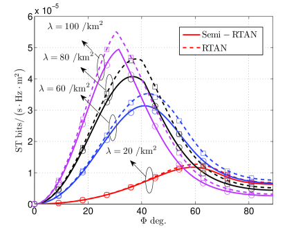
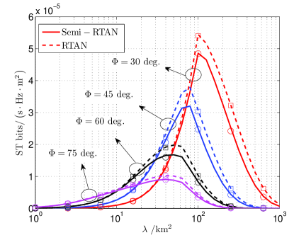
Fig. 4 plots network ST under Semi-RTNA and RTNA. In particular, Fig. 4a plots network ST with varying UAV beamwidth under different UAV deployment densities. It is observed that increasing the UAV beamwidth could first enhance network ST since a greater air-to-ground coverage could be provided. Nevertheless, network ST will be degraded due to the dominant air-to-ground interference if UAV beamwidth further increases. Meanwhile, it is shown in Figs. 4a and 4b that a greater network ST can always be obtained under RTNA. Moreover, the optimal UAV beamwidth, which maximizes the network ST, inversely grows with the UAV deployment density. This indicates that the optimal UAV beamwidth is critically dependent on the UAV deployment density.

It is shown in Fig. 4 that appropriately decreasing the UAV beamwidth could reduce the overlap of UAV projection areas and therefore is of great potential in mitigating the inter-cell interference and enhancing network ST. For this reason, we study how to optimize the UAV beamwidth in the following.

In this part, we intend to maximize the network ST through tuning the UAV beamwidth. To this end, we first formulate the optimization problem as follows.

From Propositions 3 and 4, it is shown that the UAV half-beamwidth $\Phi$ has a complicated impact of network ST under either Semi-RTNA or RTNA rule. As a consequence, it is difficult to obtain a closed-form solution for the optimal half-beamwidth $\Phi^{*}$. Even if the optimization problem in (24) is of single variable, numerically solving it may consume much time in practical applications. On this account, we propose a simple but effective PAE policy to tune the UAV beamwidth in the following.

It is shown in Fig. 4a that the optimal UAV beamwidth, which maximizes network ST, always decreases with the UAV deployment density. Moreover, it can be readily shown from (10) that the average 2D UAV-GU distance $\bar{r_{0}}$ follows $\bar{r_{0}}\propto\frac{1}{\sqrt{\lambda}}$. Therefore, the concept of the PAE policy is that the UAV projection radius $R_{\mathrm{p}}$ should be inversely proportional to the square of activated UAV density $\lambda_{\mathrm{a}}$⁵⁵5Note that no coverage will be provided by the inactivated UAVs, which are connected by no GUs.. Especially, we have

where $C\left(>0\right)$ is defined as the projection scaling parameter. A greater $C$ will result in a greater projection radius and equivalently UAV beamwidth. Therefore, supposing that the density of UAV APs is small and inter-cell interference is moderate, increasing $C$ would greatly increase the coverage of UAV APs and improve the UAV network performance. Following (25), the half-beamwidth of UAV is tuned as $\Phi^{*}=\arctan\left(\frac{C}{\Delta h\sqrt{\lambda_{\mathrm{a}}}}\right)$. Note that the projection radius of each UAV could be identically set as (25) through adjusting the beamwidth even if UAVs are in different flight altitudes. Moreover, perfect CSI is not required by the PAE policy. Therefore, the proposed policy can be applied in practical fixed-wing UAV networks, where it is difficult to acquire perfect CSI due to the high mobility of UAVs.

Since RTNA outperforms Semi-RTNA in terms of network ST, we then verify the efficiency of the PAE policy in improving network ST under RTNA. In particular, we study the scaling behavior of network ST with the growing UAV deployment density.

Proof: Please refer to Appendix A-H.∎

According to Theorem 1, we further study the network ST scaling behavior in the following two cases.

1) Backhaul unlimited case. This case occurs when sufficient backhaul could be provided through mmWave and GU density is limited. Accordingly, (26) in Theorem 1 degenerates into

where (a) follows because $\lambda_{\mathrm{a}}=q_{\mathrm{a}}\lambda$ and $\underset{\lambda\rightarrow\infty}{\mathrm{lim}}q_{\mathrm{a}}=\lambda_{\mathrm{GU}}/\lambda$ according to (6). It is shown in (27) that network ST will linearly increase with the GU density $\lambda_{\mathrm{GU}}$. This indicates that greater network ST could be obtained if more GUs request service from UAVs. In other words, the proposed PAE policy could sustainably improve spectrum reuse as long as sufficient wireless backhaul is provided. This is fundamentally different from the cases in Figs. 3 and 4b, where network ST is degraded by over-deployment of UAVs supposing that constant-beamwidth directional-antenna is equipped by each UAV.

More importantly, it is shown in (27) that identical network ST can be obtained even if UAVs are in different altitudes with the application of the proposed PAE policy. For this reason, the optimization of beamwidth could help compensate for the loss of network ST, which is due to the increase flight altitude.

2) Backhaul limited case. This case occurs when either limited backhaul could be provided or GU density is sufficiently large. According to Theorem 1, (26) degenerates into

In this case, it is observed from (28) that network ST is limited by the mmWave link capacity and mmWave effective function, which is dependent on the UAV flight altitude and hover radius (see Section II-D). According to Lemma 1, $G_{\mathrm{m}}\left(\vartheta\right)F_{\left|\varepsilon\right|}\left(\vartheta\right)$ is a decreasing function of $\vartheta=2\arctan\left(\frac{R_{\mathrm{h}}}{h_{\mathrm{UAV}}}\right)$. Therefore, the convergence value of network ST can be improved by increasing the flight altitude under the PAE policy in the backhaul-limited case.

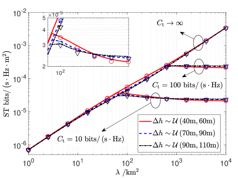
Finally, we verify the efficiency of the proposed beamwidth optimization policy. In particular, Fig. 5 plots network ST as a function of UAV density under RTNA. Compared to the results in Fig. 4b, network ST could linearly increase and then converge with the growing UAV density when RTNA is applied under the PAE policy. Moreover, even if UAVs are deployed over different altitudes, identical network ST could be obtained supposing that the backhaul capacity is sufficiently large, i.e., $C_{\mathrm{t}}\rightarrow\infty$, which verifies the validity of the results in (27). Otherwise, when backhaul capacity is limited (see the lines under $C_{\mathrm{t}}=10\mathrm{bits/\left(\mathrm{s}\cdot\mathrm{Hz}\right)}$ or $C_{\mathrm{t}}=100\mathrm{bits/\left(\mathrm{s}\cdot\mathrm{Hz}\right)}$ in Fig. 5), increasing the flight altitude could enhance network ST under large UAV deployment density.

In practice, the UAV flight altitude has to be raised in specific scenarios such as emergency and cooperative engagement, which is detrimental to the spatial reuse of available spectrum resources. However, the proposed simple but effective PAE policy could significantly enhance the spatial reuse in higher flight altitude considering both backhaul unlimited and backhaul-unlimited cases. Moreover, it is worth noting that the PAE policy could be feasibly applied in the multi-antenna system [29, 30], where UAV APs are equipped with multiple antennas. The principle of PAE and multi-antenna techniques such as coordinated beamforming is to enhance the desired signal power and alleviate the interference power received at the intended receiver. The difference is that received power distribution will be different and accordingly the UAV beamwidth should be further optimized, which is dependent on the applied multi-antenna techniques.

References

- [1] S. Koulali, E. Sabir, T. Taleb, and M. Azizi, “A green strategic activity scheduling for UAV networks: A sub-modular game perspective,” IEEE Commun. Mag., vol. 54, no. 5, pp. 58–64, May. 2016.
- [2] Y. Dong, M. Z. Hassan, J. Cheng, M. J. Hossain, and V. C. M. Leung, “An edge computing empowered radio access network with UAV-mounted FSO fronthaul and backhaul: Key challenges and approaches,” IEEE Wireless Commun., vol. 25, no. 3, pp. 154–160, Jun. 2018.
- [3] N. Zhao, F. R. Yu, L. Fan, Y. Chen, J. Tang, A. Nallanathan, and V. C. M. Leung, “Caching unmanned aerial vehicle-enabled small-cell networks: Employing energy-efficient methods that store and retrieve popular content,” IEEE Veh. Technol. Mag., vol. 14, no. 1, pp. 71–79, Mar. 2019.
- [4] J. Liu, M. Sheng, R. Lyu, and J. Li, “Performance analysis and optimization of UAV integrated terrestrial cellular network,” IEEE Internet Things Journal, vol. 6, no. 2, pp. 1841–1855, Apr. 2019.
- [5] M. Erdelj, E. Natalizio, K. R. Chowdhury, and I. F. Akyildiz, “Help from the sky: Leveraging UAVs for disaster management,” IEEE Pervasive Comput., vol. 16, no. 1, pp. 24–32, Jan. 2017.
- [6] Huawei, “5G: Huawei and Vodafone achieve 20 Gbps for single-user outdoor at E-band,” Huawei, Tech. Rep., 2016. [Online]. Available: http://www.huawei.com/en/press-events/news/2016/7/huawei-vodafone-5g-test
- [7] M. Mozaffari, A. Taleb Zadeh Kasgari, W. Saad, M. Bennis, and M. Debbah, “Beyond 5G with UAVs: Foundations of a 3D wireless cellular network,” IEEE Trans. Wireless Commun., vol. 18, no. 1, pp. 357–372, Jan. 2019.
- [8] F. Cheng, S. Zhang, Z. Li, Y. Chen, N. Zhao, F. R. Yu, and V. C. M. Leung, “UAV trajectory optimization for data offloading at the edge of multiple cells,” IEEE Trans. Veh. Technol., vol. 67, no. 7, pp. 6732–6736, Jul. 2018.
- [9] A. V. Savkin and H. Huang, “Deployment of unmanned aerial vehicle base stations for optimal quality of coverage,” IEEE Wireless Commun. Lett., vol. 8, no. 1, pp. 321–324, Feb. 2019.
- [10] X. Sun and N. Ansari, “Latency aware drone base station placement in heterogeneous networks,” in Proc. IEEE GLOBECOM, Singapore, Dec. 2017, pp. 1–6.
- [11] C. Zhang and W. Zhang, “Spectrum sharing for drone networks,” IEEE J. Sel. Areas Commun., vol. 35, no. 1, pp. 136–144, Jan. 2017.
- [12] KDDI, “Terra drone, KDDI launch new UAS services,” KDDI, Tech. Rep., 2019.
- [13] AT&T, “When COWs fly: At&t sending LTE signals from drones,” AT&T, Tech. Rep., 2019. [Online]. Available: https://about.att.com/innovationblog/cows_fly
- [14] Y. Zeng and R. Zhang, “Energy-efficient UAV communication with trajectory optimization,” IEEE Trans. Wireless Commun., vol. 16, no. 6, pp. 3747–3760, Jun. 2017.
- [15] S. Jeong, O. Simeone, and J. Kang, “Mobile edge computing via a UAV-mounted Cloudlet: Optimization of bit allocation and path planning,” IEEE Trans. Veh. Technol., vol. 67, no. 3, pp. 2049–2063, March 2018.
- [16] J. Zhou, Y. Su, and P. Li, “An emergency mobile communication system based on fixed-wing drone and satellite transmission access,” in Proc. IEEE DASC/PiCom/CBDCom/CyberSciTech, Fukuoka, Japan, Aug. 2019, pp. 465–470.
- [17] R. He, B. Ai, G. L. Stüber, G. Wang, and Z. Zhong, “Geometrical-based modeling for millimeter-wave MIMO mobile-to-mobile channels,” IEEE Trans. Veh. Technol., vol. 67, no. 4, pp. 2848–2863, Apr. 2018.
- [18] R. He, B. Ai, G. Wang, Z. Zhong, C. Schneider, D. A. Dupleich, R. S. Thomae, M. Boban, J. Luo, and Y. Zhang, “Propagation channels of 5G millimeter-wave vehicle-to-vehicle communications: Recent advances and future challenges,” IEEE Veh. Technol. Mag., vol. 15, no. 1, pp. 16–26, Mar. 2020.
- [19] G. Wang, Q. Liu, R. He, F. Gao, and C. Tellambura, “Acquisition of channel state information in heterogeneous cloud radio access networks: challenges and research directions,” IEEE Wireless Commun., vol. 22, no. 3, pp. 100–107, Jun. 2015.
- [20] Z. Yang, C. Pan, M. Shikh-Bahaei, W. Xu, M. Chen, M. Elkashlan, and A. Nallanathan, “Joint altitude, beamwidth, location, and bandwidth optimization for UAV-enabled communications,” IEEE Commun. Lett., vol. 22, no. 8, pp. 1716–1719, Aug. 2018.
- [21] H. Zhu and J. Wang, “Chunk-based resource allocation in OFDMA systems - part I: chunk allocation,” IEEE Trans. Commun., vol. 57, no. 9, pp. 2734–2744, Sep. 2009.
- [22] ——, “Chunk-based resource allocation in OFDMA systems - part II: Joint chunk, power and bit allocation,” IEEE Trans. Commun., vol. 60, no. 2, pp. 499–509, Feb. 2012.
- [23] J. Wildman, P. H. J. Nardelli, M. Latva-aho, and S. Weber, “On the joint impact of beamwidth and orientation error on throughput in directional wireless poisson networks,” IEEE Trans. Wireless Commun., vol. 13, no. 12, pp. 7072–7085, Dec. 2014.
- [24] W. Feng, Y. Li, D. Jin, L. Su, and S. Chen, “Millimetre-wave backhaul for 5G networks: Challenges and solutions,” IEEE Trans. Veh. Technol., vol. 16, no. 2, p. 892, Jun. 2016.
- [25] B. Ejder, B. Mehdi, K. Marios, and D. Mérouane, “Cache-enabled small cell networks: modeling and tradeoffs,” EURASIP J. Wireless Commun. Netw., vol. 2015, no. 1, pp. 1–11, Feb. 2015.
- [26] Z. Yan, S. Chen, Y. Ou, and H. Liu, “Energy efficiency analysis of cache-enabled two-tier hetnets under different spectrum deployment strategies,” IEEE Access, vol. 5, pp. 6791–6800, Mar. 2017.
- [27] S. Lee and K. Huang, “Coverage and economy of cellular networks with many base stations,” IEEE Commun. Lett., vol. 16, no. 7, pp. 1038–1040, Jul. 2012.
- [28] E. Turgut and M. C. Gursoy, “Energy efficiency in relay-assisted mmWave cellular networks,” in Proc. IEEE VTC-Fall, Montreal, Canada, Sep. 2016, pp. 1–5.
- [29] C. Xing, S. Ma, and Y. Zhou, “Matrix-monotonic optimization for MIMO systems,” IEEE Trans. Signal Process., vol. 63, no. 2, pp. 334–348, Jan. 2015.
- [30] Y. Dong, M. J. Hossain, J. Cheng, and V. C. M. Leung, “Cross-layer scheduling and beamforming in smart-grid powered cellular networks with heterogeneous energy coordination,” IEEE Trans. Commun., to be published.
- [31] M. Haenggi and R. K. Ganti, Interference in large wireless networks. Now Publishers Inc, 2009.
- [32] F. Eriksson, “The law of sines for tetrahedra and n-simplices,” Geometriae Dedicata, vol. 7, no. 1, pp. 71–80, 1978.
- [33] D. Stoyan, W. S. Kendall, J. Mecke, and L. Ruschendorf, Stochastic geometry and its applications. Wiley Chichester, 1995, vol. 2.
- [34] J. Liu, M. Sheng, L. Liu, and J. Li, “Effect of densification on cellular network performance with bounded pathloss model,” IEEE Commun. Lett., vol. 21, no. 2, pp. 346–349, Feb. 2017.