Accelerating ViT Inference on FPGA through Static and Dynamic Pruning
Abstract
Vision Transformers (ViTs) have achieved state-of-the-art accuracy on various computer vision tasks. However, their high computational complexity prevents them from being applied to many real-world applications. Weight and token pruning are two well-known methods for reducing computational complexity. Weight pruning reduces the model size and associated computational demands, while token pruning further reduces the computation based on the input. Combining these two techniques should significantly reduce computation complexity and model size; however, naively integrating them results in irregular computation patterns, leading to significant accuracy drops and difficulties in hardware acceleration.
To address the above challenges, we propose a comprehensive algorithm-hardware codesign for accelerating ViT on FPGA through simultaneous pruning – combining static weight pruning and dynamic token pruning. For algorithm design, we systematically combine a hardware-aware structured block-pruning method for pruning model parameters and a dynamic token pruning method for removing unimportant token vectors. Moreover, we design a novel training algorithm to recover the model’s accuracy. For hardware design, we develop a novel hardware accelerator for executing the pruned model. The proposed hardware design employs multi-level parallelism with a load-balancing strategy to efficiently deal with the irregular computation pattern led by the two pruning approaches. Moreover, we develop an efficient hardware mechanism for executing the on-the-fly token pruning. We apply our codesign approach to the widely used DeiT-Small model. We implement the proposed accelerator on a state-of-the-art FPGA board. The evaluation results show that the proposed algorithm can reduce computation complexity by up to with accuracy drop and a model compression ratio of up to . Compared with state-of-the-art implementation on CPU, GPU, and FPGA, our codesign on FPGA achieves an average latency reduction of , , and , respectively.
Index Terms:
Vision transformer, model pruning, hardware accelerationI Introduction
Vision Transformers (ViTs) [1] have demonstrated superior performance in comparison to Convolutional Neural Networks (CNNs) in various vision tasks [2, 3, 4, 5, 6, 7, 8]. The global self-attention in ViTs leads to a reduced local and image-specific inductive bias [1]; this results in ViTs requiring larger datasets and larger model sizes [9] to perform better than CNN. The Multi-head Self-Attention (MSA) of ViTs allows them to generalize better than CNNs on larger datasets [10]. However, their computational cost is usually significantly higher than CNNs due to the MSA mechanism, which scales quadratically with the number of input tokens [11, 12]. Their intensive computational requirements emphasize the need for efficient hardware acceleration.
In addressing the computational challenge, pruning has been proven to be effective in reducing the computational cost of CNNs [13, 14, 15, 16]. However, explorations in self-attention-based pruning methods still need to be discovered [17, 18, 19]. Many existing works on efficient ViTs explored block weight pruning and token pruning as two distinct strategies. Weight pruning, introduced in [20, 21, 22, 23, 17, 24, 18, 25, 25, 26], reduces the model size by pruning input parameters statically and selectively, thus feeding the neural network with sparse inputs to reduce computation. Token pruning removes tokens to reduce the computational complexity. The static approaches in [27, 28, 29, 30] drop tokens with a fixed ratio, often ignoring the redundancies between tokens; dynamic token pruning studies in [31, 32, 33] do not fully explore the token redundancies from different attention heads and simply discard non-informative tokens. [34, 35, 36, 37] dynamically reduce the number of tokens in ViT encoders during inference based on the inherent image characteristics. Moreover, only a few of these studies support efficient hardware implementations by the respective pruning algorithm. Both weight pruning and token pruning methods reduce the computational complexity independently, but the interaction between the two remains unexplored. A combined approach could bring further computational benefits. However, such integration poses two main challenges: (1) accuracy drop (algorithm level) and (2) increased computational pattern irregularities (hardware level).
Many ViT acceleration works primarily focus on the CPU and GPU platforms [28, 36, 32, 29, 30]. However, the integration of block weight pruning and token pruning in ViTs effectively reduces the model size, thus making it possible to accommodate the compressed model onto FPGA. Comprehensively, we use FPGA to accelerate our pruned ViT models for these reasons: (1) FPGAs, with customized data path and on-chip memory organization, stand out as better choices than CPU/GPU to maximize the computation efficiency. (2) CPUs and GPUs cannot effectively handle the token shuffling process of our dynamic token pruning. We design a specific FPGA kernel to handle the token shuffling in the middle of model inferences. (3) CPUs and GPUs need complicated processes to address work-load imbalance, whereas on FPGA, we can design customized hardware modules for balancing work-load.
In this paper, we propose an algorithm-hardware codesign for accelerating ViT inference. Different from existing ViT acceleration works, we utilize the combined power of static weight pruning and dynamic token pruning. We propose a simultaneous pruning algorithm to recover the model accuracy caused by two pruning approaches. Combining the two pruning approaches leads to more severe computational irregularity. Therefore, we develop a customized data path and memory organization on FPGA to execute the pruned model efficiently. While existing ViT accelerators on FPGA [35, 37] can handle the irregular patterns after pruning, they target either weight pruning or token pruning, but not both. Therefore, none of the existing FPGA ViT accelerators can support our integrated simultaneous pruning approach. We summarize our main contributions below:
-
•
We propose an algorithm-hardware codesign for efficient ViT inference based on FPGA. The design combines parameter (static) and token (dynamic) pruning to reduce both the ViT model size and computational complexity.
-
•
For the algorithm design, we systematically combine static block weight pruning and dynamic token pruning to reduce the computation complexity of ViTs. We propose a novel training algorithm to recover the accuracy drop led by the two pruning algorithms.
-
•
For the hardware design, we develop a novel hardware accelerator with multi-level parallelism and a load balancing strategy. This can efficiently deal with (1) load imbalance caused by the block pruning and (2) a changing number of tokens caused by token pruning. We also develop an efficient hardware mechanism for executing the on-the-fly token pruning algorithm.
-
•
We evaluate our codesign on DeiT models and deploy the proposed accelerator on a state-of-the-art FPGA board - Xilinx Alveo U250. The evaluation results show that the proposed algorithm can reduce computation complexity by up to with accuracy drop and a model compression ratio of up to . Compared with state-of-the-art implementation on CPU, GPU, and FPGA, our codesign on FPGA achieves average latency reduction of , , respectively.
II Background and Related Work
II-A Vision Transformer
ViT [1] has a stack of transformer encoders. Each encoder has a multi-head self-attention (MSA) and a multi-layer perceptron (MLP). The input image is first partitioned into patches . Each patch is flattened into a vector of length . Next, a learnable linear mapping method maps each patch to a token vector of length . A special parameterized token is appended as a token vector. Then, a positional embedding is added to input token matrix to produce which is the input to the transformer encoder stack. For simplicity, we denote the number of input tokens to the encoder stack as instead of for the rest of the paper.
MSA. The input to encoder , is layer normalized (LN) [38] and passed through a multi-headed self-attention (MSA) layer [12]:
| (1) |
is expressed as:
| (2) |
where , , , corresponding to query, key and value matrices, respectively. is the length of input token and is the hidden dimension. Then, the attention score matrix is calculated through:
| (3) |
| (4) |
refers to self-attention with a single head. extends this notion of self-attention to several parallel heads, each with its own parameters:
| (5) |
where denotes the total number of heads. projects the concatenated self-attention outputs of the individual heads back to the embedding dimension .
MLP. The output of MSA, is layer normalized and passed through a multi-layer perceptron (MLP):
| (6) |
II-B Related Work
Weight pruning: Structured and hardware-friendly model parameter pruning, used in traditional CNNs [20, 21, 22], becomes popular for ViT. [17] introduces the notion of movement pruning, which prunes parameters by generating a pruning mask based on the learned scores. [23] proposes to prune parameters across all the encoders. Magnitude-based approaches, on the other hand, discard parameters with large magnitudes [24]. [18] partitions a parameter matrix into blocks and prunes the rows and columns in each block by using the norms. [25] prunes the entire attention heads within the MSA and neurons in each feed-forward linear layer (width pruning). [25] also removes entire encoders after a certain depth (depth pruning). [26] proposes a collaborative approach to optimizing ViT pruning that prunes heads and neurons; the latter neurons are pruned such that they reduce the length of each token. This method considers the collective pruning impact through an expensive approximation of the Hessian of the loss.
Token pruning: Token pruning approaches attempt to identify redundant tokens and drop them to reduce the computational footprint associated with the number of tokens. Both [19] and [39] have been notable for accelerating transformer models by leveraging the inherent sparsity in attention mechanisms. However, they do not use weight and token pruning simultaneously. [28] proposes a static approach to token dropping that ranks the importance of tokens by the attention score of the class token with respect to each token aggregated across heads. In theory, such static approaches do not need additional training since the token-dropping module is not parameterized. In contrast to static token pruning, dynamic token pruning as employed in [36, 35, 34] adds additional model parameters that facilitate the selection of relevant/attentive tokens. [36] and [35] utilize a token selector network inserted at various depths along the original transformer network; such token selector networks are neural networks that output a decision (binary) mask to inform the retention or removal of a token. [34], on the other hand, associate a learnable score to each token and prune tokens with scores lower than a threshold.
III Overview
III-A Problem Definition
Our objective is to accelerate ViT on FPGA through an algorithm-hardware codesign that 1) utilizes a novel combination of model weight pruning and token pruning to reduce computation complexity (algorithm design), and 2) an efficient accelerator that explicitly accounts for the distinct and irregular access patterns of the two pruning techniques for executing the combined pruned model (hardware design).
For the algorithm design, the input is a ViT model denoted as where are the model hyper-parameters, including the number of encoders, number of heads, dimensions of linear layers, etc. is the trainable parameters containing the weights and biases of the MSA and MLP. Our algorithm design prunes the input model through (1) offline weight pruning that reduces the redundant parameters in , and (2) runtime token pruning that trims the number of tokens (in ) in the intermediate layers according to the importance of the token. After pruning, we obtain the pruned model denoted as , where denotes the model parameters after weight pruning and denotes the hyperparameters after token pruning. Our algorithm design aims to reduce the number of parameters, reduce the computation complexity, and maintain accuracy.
For the hardware design, the hardware accelerator executes the pruned model . For executing the model, the input is an image sample , and the accelerator executes to obtain the result. The latency is the duration from the time when the accelerator receives the input to the time when the accelerator obtains the result.
III-B Computational Complexity
The computational complexity for each operation within the MSA and MLP without pruning are summarized in table I. denotes the batch size.
Operation Computational Complexity LayerNorm Residual Add MSA MLP Total Complexity
III-C Overview of Algorithm-hardware Codesign
The overview of the proposed codesign is shown in Figure 1, which consists of algorithm design and hardware design.
Algorithm design: For algorithm design, we utilize the combination of block-wise static weight pruning (Section IV-A) and input token pruning (Section IV-B). The input is the input ViT model and the pruning hyper-parameters (including the weight pruning ratio for each layer and token pruning ratio for each layer). Users manually specify the pruning hyper-parameters. Then, the proposed simultaneous pruning (training) algorithm (Section IV-C) prunes the input model according to the user-specified pruning hyper-parameters. Then, the pruned model is generated. The model optimizations organize the data blocks in the weight matrices into the required data layout and format (Section V-A) for efficient hardware execution on the proposed accelerator.
Hardware accelerator design: At runtime, when the host process receives an input image, it sends the input image to the accelerator for inference. We employ a multi-level parallelism strategy for the proposed hardware architecture to efficiently handle the irregular computation patterns. We design a Token Dropping Hardware Module for efficient on-the-fly token dropping. See Section (Section V-C) for details.
Discussion on the challenges of hardware acceleration: The combination of two pruning approaches leads to significant challenges for hardware accelerations: (1) Through weight pruning, the weight matrix of MSA has uneven number of data blocks among different columns and different layers can have different number of heads. Moreover, the token pruning leads to varying number of tokens for different layers. These potentially leads to runtime resource underutilization. We address this challenge through multi-level parallelism (Section V-C) with load balance strategy (Section V-D). (2) Due to the block-wise weight pruning, both token matrix and weight matrices are partitioned into data blocks. However, the token dropping algorithms drops unimportant tokens in the intermediate layers. Therefore, the token matrix needs to be reordered and reconstructed on the fly based on their importance score. This involves sorting and data shuffling which cannot be efficiently handled by CPU or GPU. We develop efficiently hardware mechanism in Token Dropping Hardware Module to address the above issue (Section V-C3).

IV Pruning Algorithm
Existing works only utilize either weight pruning or token pruning. In contrast, we systematically combine the two pruning approaches with a novel training algorithm for recovering accuracy. To this end, we first introduce static weight pruning (Section IV-A) and dynamic token pruning (Section IV-B) separately, and then introduce our Simultaneous Pruning algorithm to prune the input model.
IV-A Static Weight Pruning
The weights to be pruned are: weight matrices for , , and within MSA and the intermediate and output linear layers within MLP. Pruning is performed as follows:
IV-A1 Pruning of MSA
We use , , to denote the concatenation of weight matrices of all the heads. For example, The projection operation (Equation 5) projects the concatenated SA outputs of embedding dimension back to dimension via . To prune a weight matrix , we define a parameterized score matrix such that, where is the block size. denotes the importance score of a parameter block of size in the weight matrix denoted by the slice where . is used to construct a mask via the top- selection:
| (7) |
wher is a block of size in corresponding to . The masked weight is generated as, where is the element-wise Hadamard product. The generated masked weight is used for the forward pass during training. Note that top- is the target weight blocks of interest. To compute the gradient of during the backward pass, a straight-through estimator (STE) [40, 41, 42] is used that neglects the gradients of with respect to . Additionally, the pruning of in row dimension and the pruning of in column dimension follows the same pattern (denoted as alternate pattern), as shown in Figure 2. For example, a head removed from makes the corresponding head in redundant, and vice-versa.

MLP Pruning. The weight matrices in MLP are . The pruning of and follows the approach for pruning MSA. A key difference, however, is in how the score parameters are defined for and . Specifically, we define the scores as: . The score vectors are defined to prune entire columns of and entire rows for (see Figure 3). Masks are generated column-wise/row-wise through top- selection. The natural parameter partitioning along the heads in MSA makes block pruning more effective in terms of removing entire heads. MLP parameters, on the other hand, lack such a partitioning. We thus focus on removing entire columns/rows for MLP parameters. For model training, we add a norm of the sigmoid of scores to the training loss [23]:
| (8) |
where the loss is updated to penalize the presence of a model parameter, thus driving the model to be sparse. The extent of this penalization is controlled by the hyper-parameter .

IV-B Dynamic Token Pruning
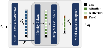
Dynamic Token Pruning prunes along the token dimension . The redundancy along the token dimension comes from the fact that several patches within an input image are inattentive, contributing insignificantly to the final learned model [35, 34, 28, 36]. Since ViTs can inherently handle inputs with an arbitrary number of tokens (patches), we exploit this independence of the input token dimension from the model parameter dimension(s) by dropping inattentive tokens. Specifically, to classify tokens into attentive and inattentive tokens, we use a non-parametric approach [28]. The attention computed within the MSA (Equation 3) is utilized to perform attentive token identification. In MSA, the attention score is generated by each head. We aggregate the above score vector across all the heads using and represents the importance score of every single token. Based on a keep-rate , a total of tokens with the top scores in are retained. The remaining inattentive tokens are fused into a single token by performing a weighted aggregation of these tokens with respect to their respective scores in . The above token dropping is performed via a token dropping module (TDM) inserted between the MSA and the MLP modules (Figure 4), with the tokens dropped dynamically during both training and inference.
IV-C Simultaneous Pruning
To recover accuracy for the pruned model, we utilize the knowledge distillation technique commonly used to transfer knowledge from an already trained larger teacher model to a smaller student model [43]. The class logits associated with the teacher and the student networks are used to compute a distillation loss at a distillation temperature :
| (9) |
where stands for the KL divergence loss. refers to the softmax probability vector computed at a temperature of from input logits vector as . The final loss is obtained as a weighted sum of the generic loss and the distillation loss, with the weights acting as hyper-parameters. The simultaneous training algorithm used to train a sparse model on sparse attentive input tokens is given in Algorithm 1. is an encoder at layer with the TDM module included, in a ViT model . Similarly, is an encoder at layer without the TDM.
IV-D Computational Complexity: Pruned Model
We analyze the computational complexity for the proposed pruned model. The complexity of an encoder is described in table II. is the average ratio of retained weight blocks to the total weight blocks (retained and pruned) within a column of blocks in parameter matrices (computed after the removal of heads pruned in their entirety). is defined similarly, but for matrix . are the number of heads retained within MSA. are the total retained tokens after token dropping (). is the ratio of retained neurons (same for both and ). Note that .
Operation Computational Complexity LayerNorm 1 () LayerNorm 2 () Residual Add 1 () Residual Add 2 () MSA () TDM () MLP () Total Complexity

V Hardware Design
In this Section, we introduce our hardware design to accelerate the pruned model on the FPGA platform. To be specific: in Section V-A, we introduce the data format and layout that store the sparse (and dense) weight matrices and input data; in Section V-B, we introduce the main components in the proposed hardware architecture. In Section V-C, we introduce the workflow for executing the pruned ViT encoder using the proposed hardware design.


V-A Data Format and Layout
Due to structured block pruning, all weight and feature matrices are partitioned into data blocks of the same size . All the data in the same blocks are stored contiguously. The dense matrix is stored in block-wise row-major order such that all the data blocks of the same row are stored contiguously in memory space. The weight matrices are stored in column-major order such that all the unpruned data blocks in the same column are stored contiguous in memory space as shown in Figure 5. Note that for the sparse weight matrices, only unpruned data blocks are stored. For each column in a block-wise sparse weight matrix, we include a header at its beginning that encodes row indices of the present blocks and the length of the column block. For simplicity, in the rest of the paper, a row of matrix denotes a row of data blocks, and a column of matrix denotes a column of data blocks.
V-B Hardware Overview
As shown in Figure 6, the architecture design comprises of: (1) Multi-level Parallelism Compute Array (MPCA), (2) Element-wise Module (EM), (3) Token Dropping Hardware Module (TDHM). Besides, there are on-chip buffers, including a Global Feature Buffer (GFB) that stores the feature matrices, (2) Column Buffers (CB) that store the weight matrix, (3) Result Buffers (RB) that store the results of the current layer.
In MPCA, the computation units are organized into multiple levels. An MPCA has parallel Computing Head Modules (CHMs). Each CHM has a 2-D array of Processing Elements (PEs) of size . Each Processing Element has an array of computation units of size . Essentially, , , , are the computation parallelism in the head dimension, input token dimension, weight column dimension, and the data parallelism within the data blocks, respectively. The Element-wise Module (EM) performs element-wise GELU and exponentiation. The Token Dropping Hardware Module (TDHM) performs dynamical token dropping (Section IV-B).
The computation units in MPCA are organized to multi-level because (1) it enables massive data parallelism in MSA and MLP, (2) it enables data reuse/sharing within CHM. The PEs in the same column of CHM can share the same weight block, while the PEs in the same rows of CHM can share the same input token block. This data-sharing strategy simplifies the computation complicated by the irregular data access pattern of block-wise weight pruning. (3) By selecting proper with a load balancing strategy, we can alleviate the load imbalance caused by block-wise weight pruning.
V-C Workflow
The proposed accelerator executes the input model layer-by-layer, with each layer being executed using the same set of computational resources (e.g., MPCA). Each CHM utilizes Sparse Block-wise Matrix Multiplication (SBMM) to process sparse matrices in blocks. For dense matrices, the computation shifts to Dense Block-wise Matrix Multiplication (DBMM) and Dense Head-wise Block Matrix Multiplication (DHBMM) for a focused computation on matrix blocks associated with each head. Each layer performs as follows:
V-C1 MSA Execution
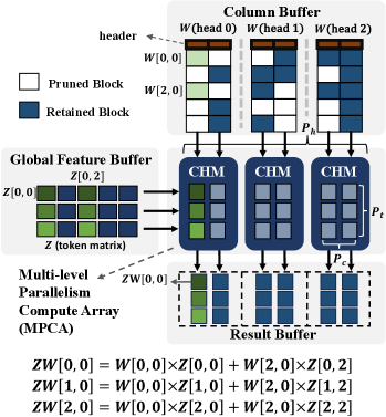
MSA is divided into four stages (shown in Figure 7): stage (i) computes , and through . is the input token matrix and is matrix concatenation. Let and denote the query, key, and value matrices for a head , where . The algorithm for executing each matrix multiplication (e.g., dense token matrix multiply by sparse weight matrices ) in MSA using MPCA is shown in Algorithm 2 and an example is shown in Figure 8. Each CHM computes its corresponding head . Since we perform block partitioning for each matrix, the computation is executed in a block-wise fashion. Within each CHM, the PEs within a column share the same column of weight, which is stored in the column buffer (CB). PEs of the same row share the same row of . We use to denote a PE in the CHM at location within the CHM. A column of PEs: share the same column of weight with the corresponding header information (See Figure 5). Thus, each PE in column utilizes the shared header indices (Figure 5) to fetch the corresponding data block from the token matrix (in the local input buffer) to perform block-wise matrix multiplication. The partial results are accumulated in local result buffers.
The stage (ii) computes the attention scores . is dense block-wise matrix multiplication executed via the MPCA module (See Algorithm 2). is buffered in the GFB, and is buffered in the CB. The output data blocks of are sent to EM module for element-wise scaling (by ) and exponentiation to obtain . Then, we utilize MPCA to compute the scaling factors for . The rows of matrix and their corresponding computed scaling factors, are streamed from MPCA to EM to perform the scaling to obtain the attention scores, .
The stage (iii) computes the self-attention . It is similar to the computation of . The stage (iv) computes the projection (Equation 5). It is similar to the computation of , and described in stage (i) as is the block-wise sparse matrix due to pruning.
V-C2 MLP Execution
Since the weights of MLP are pruned for entire columns or rows (for and respectively), MLP layers can be mapped into dense block-wise matrix-matrix multiplication executed by MPCA (Algorithm 2). This computation is similar to the computation of MSA (computing ). GELU activation is computed using the EM module.
V-C3 Dynamic Token Dropping
We design a token dropping hardware module (TDHM) for on-the-fly token dropping and reorganizing the remaining tokens. The token pruning is based on importance scores of tokens (See Secton IV-B). The attention scores for all the heads are buffered in the TDHM as soon as they are computed via MSA execution. Then, scores are computed via the EM. After that, a bitonic sorting network sorts the scores to obtain the indices of top- tokens. Original, each token has a row index in the input token matrix , denoted as old token index (). After sorting by , each token is assigned new token index () which is the row index in the output token matrix . Therefore, the sorting network generates (, , flag) for each token, where flag indicates if the token will be pruned. To organize output token matrix (stored in Old Token Buffer), an index shuffle network routes each flag to Old Token Buffer for fetching tokens according to . Then, the fetched tokens are routed to the New Token Buffer according to , which generates too- token matrix and non-top- token matrix. The non-top- tokens are then fused into a single token and merged with the top- tokens to produce the output of TDHM module.
V-D Optimizations
V-D1 Load balancing across columns for SBMM
As the weight matrices are pruned in block-wise fashion, different columns in a weight matrix can have different number of data blocks, which can potentially lead to load imbalance. The multi-level parallelism in MPCA distributes the PEs across several heads (CHMs). PEs within each CHM computes on weight column blocks using multiple iterations that each iteration executes different columns of weight matrices (See Algorithm 2). This naturally reduces the impact of load imbalance due to differing sparsity levels across the columns of weight matrices. As we restrict block-wise pruning to only the weights of MSA (, , , ), this further reduces the impact of load imbalance. Note that the gain in performance by block-wise pruning the MSA parameters (leading to the removal of entire heads) is far outweighted by the load imbalance presented by such pruning. Prior methods [44] that balance such block-wise pruning across columns are disadvantaged by the fact that they cannot remove entire heads. Moreover, we perform offline workload assignment among columns of weight marices, prior to inference, such that workloads of columns are evenly distributed across different columns of PEs within a CHM.
V-D2 Dealing with varying number of tokens, retained heads and block sizes
Dynamic token pruning, leads to varying number of tokens for different layers. Moreover, block-wise weight pruning the MSA parameters leads to removal of heads within an encoder. In general, the heads removed or retained in each encoder can vary, which can potentially lead to runtime hardware underutilization. For example, if the number of rows of token matrix , rows of PEs in a CHM will be idle. As we utilize multi-level parallelism in MPCA, through selecting proper (parallelism in token dimension) and (parallelism in head dimension), we can alleviate the underutilization. We use to denote the minimum number of row blocks of all the intermediate token matrices and use to denote the minimum number of heads of all the layers. Through setting , the PEs utilization in a CHM will be (Suppose . The utilization will be ). Similar, we can set .
V-E Resource and Performance Models
V-E1 Resource Consumption Model
We perform theoretical analysis for the performance achieved by the codesign and its hardware resource utilization. We denote the total computational resources utilized by the MPCA, EM and TDHM as and , respectively. is proportional to the total number of computation units: . Compared to , the resources used by and are negligible, and thus ignored for analysis. The total (DSPs and LUTs) are , where and denote the amount of DSPs and LUTs utilized by a single computation unit. The size of the (global) feature buffer, column buffer and the (global) result buffer, associated with the MPCA, are , and , respectively. Here, is the block size and is a constant that equals the (maximum) total number of row blocks required to compute a single output block. We match the buffer sizes across compute units to improve the dataflow performance of the accelerator. This gives a total buffer size of for the EM module and for the TDHM module. The EM module requires a buffer to store the input, scaling factor, addtion factor and the output. Similarly, TDHM requires an input and an output buffer. The total size of required buffers is given as, . and are the estimation of resource utilization. The main design , and , with are empirically set according the resource of target FPGA platform (See Section VI for details).
V-E2 Performance Model
Based on algorithm 2, the number of cycles to perform either SBMM, DBMM or DHBMM is estimated in table III. Note that DHBMM is DBMM computed head-wise (as in stage (ii) of MSA execution). In table III, the cycles for SBMM/DBMM are the cycles required to multiply a matrix of dimension with a matrix of dimension . is the size per head, is the block size and is the ratio of retained dense blocks to total blocks within a column of the matrix. Note that for DBMM, is and for SBMM, is assumed similar in each column block for simplicity. and are the per head left and right matrix sizes, for DHBMM, with being the total number of heads. The cycle estimates in Table III can be used to compute the total cycles for the MSA and the MLP blocks.
| Cycles | |
|---|---|
| SBMM/DBMM | |
| DHBMM |
VI Implementation Details
Evaluated Model: We evaluate our approach on the widely used DeiT-Small [45] model, which has 12 layers, with each layer having six heads. The hidden dimension is , and the (base) model has M parameters.
Implementation details of weight pruning, token pruning, and simultaneous training: The DeiT-Small model is simultaneously pruned as per algorithm 1. We train several variants of the model by varying the model pruning top- rate , token pruning keep rate , and block size . Specifically, is varied over , over and over . A cubic sparsity scheduler, as in [17], is used to schedule from a full density of to its final density ( or ) with a warm-up and a cool-down phase. The token-dropping module, TDM, is inserted in the , and encoder layers. All model variants are trained for a total of epochs using the AdamW optimizer [46] with a learning rate of , weight decay of and a batch size of across GPUs. Note that to train all pruned variants as well as the baseline, we use the pre-trained DeiT-Small model available at [47] with the classification MLP head parameters re-initialized. A ViT base model is used as the teacher for knowledge distillation.
Hardware implementation details: We implement our FPGA design on a state-of-the-art FPGA platform, Xilinx Alveo U250, which consists of four Super Logic Regions (SLRs). We implement the proposed hardware design using Xilinx High-level Synthesis (HLS). For the MPCA module, we empirically determine the hardware hyperparameters to be , , , according to the hardware resources of the target FPGA board: (1) We set because Alveo u250 has four SLRs, with each SLR placed in one CHM. (2) We set because in a CHM, the PEs of the same row load the same rows of tokens but different data blocks. The BRAM/URAM on FPGA has two independent memory ports, which can support concurrent memory access of columns of PEs (). (3) We set because the data block size is set as or for block-wise weight pruning. Using can support these two block sizes without data padding as well as keeping a reasonable value for . (4) For setting , the PEs of the same column within a CHM shares the same weight blocks. The weight blocks are broadcast into each PE of the same column, which supports any value of . We set according to the available resources of the target FPGA board after determining , , and . We use the int16 data format. We utilize the four DDR4 channels of U250, which have 77 GB/s of external memory bandwidth in total. We perform synthesis and place-route for the design using Xilinx Vitis v2022.2. We report the frequency and FPGA resource utilization after place-route. The achieved frequency is MHz, and the resource utilization is shown in Table IV.
VII Experiments and Results
VII-A Baselines, Metrics, Datasets
Baselines: We compare our implementation on FPGA with the state-of-art CPU, GPU, and FPGA accelerators including [37] and [49]. Table V shows the details of these platforms.
CPU GPU HeatViT [37] SPViT [35] Our work Platform AMD EPYC 9654 NVIDIA RTX 6000 Ada Xilinx ZCU102 Xilinx ZCU102 Xilinx Alveo U250 Frequency 2.4 GHz 915 MHz 150 MHz 200 MHz 300 MHz Peak Performance (TFLOPS) 3.69 91.06 0.37 0.54 1.8 On-chip Memory 384 MB 96MB 3.6MB 4MB 36 MB Memory Bandwidth 461 GB/s 960 GB/s 19.2 GB/s 19.2 GB/s 77 GB/s
Datasets: Following prior works [28][37], we use ImageNet dataset in our experiments with approximately 1.2 million images to evaluate our approach.
Performance Metrics: We utilize the following performance metrics: (1) Accuracy: Following prior works, we evaluate the accuracy of our pruned model on ImageNet. (2) Inference latency: Following prior works [37, 49, 35], we measured inference latency via hardware emulation using AMD-Xilinx Vitis, which accurately simulates the behavior of FPGA DDR. The measured latency is end-to-end from the time when the input is given at DDR to the time when the inference result is written back to DDR. (3) Throughput: Throughput denotes the number of images that can be processed for a given time frame. (4) Computation complexity (FLOPS): We measure the computational complexity, which is the number of floating-point operations (FLOPs). (5) Model size: The amount of memory space (MB) to store the model.
Notion Block Pruning Token Pruning Head Retained Ratio Model Parameters Training Epochs Accuracy FPGA Latency (ms) FPGA Throughput (images/second) Block Size Top- Rate Token Keep Rate Model Size MACs (Baseline) 16 1 1 1 22M 4.27G 30 79.59% 3.19 313.00 (Baseline) 32 1 1 1 22M 4.27G 30 79.59% 3.55 281.43 (Pruned) 16 0.5 0.5 0.91 14.29M 1.32G 30 66.86% 0.868 1151.55 (Pruned) 16 0.5 0.7 0.91 14.29M 1.79G 30 68.62% 1.169 855.12 (Pruned) 16 0.5 0.9 0.93 14.39M 2.43G 30 70.14% 1.479 676.10 (Pruned) 16 0.7 0.5 0.98 17.63M 1.62G 30 74.12% 1.140 877.054 (Pruned) 16 0.7 0.7 0.98 17.63M 2.20G 30 75.96% 1.553 643.72 (Pruned) 16 0.7 0.9 0.98 17.63M 2.98G 30 76.55% 1.953 511.94 (Pruned) 32 0.5 0.5 0.84 13.80M 1.25G 30 67.25% 1.621 616.79 (Pruned) 32 0.5 0.7 0.83 13.70M 1.70G 30 68.62% 1.796 556.66 (Pruned) 32 0.5 0.9 0.84 13.80M 2.31G 30 70.06% 1.999 500.17 (Pruned) 32 0.7 0.5 0.97 17.53M 1.61G 30 73.45% 2.126 470.33 (Pruned) 32 0.7 0.7 0.94 17.33M 2.16G 30 75.65% 2.353 424.93 (Pruned) 32 0.7 0.9 0.94 17.33M 2.93G 30 76.40% 2.590 386.02
VII-B Evaluation for the Pruning Algorithm
Results in Table VI indicate that for extreme pruning settings (, both ), the accuracy drop () compared against the baseline is not insignificant. A major reason for this drop is the fact that the training epochs for our experiments were restricted to despite the reduction in model and input density. With a lower top- rate and token keep rate , the model requires larger epochs to converge. Compared to the baseline DeiT-Small model, the proposed simultaneous pruning algorithm achieves a compression ratio of up to to and a reduction in the computational cost of up to to with an accuracy drop of as little as . Whilst prior works focus on either reducing the model size [44] or on reducing the computational complexity [37, 35], our proposed simultaneous pruning algorithm targets both.
VII-C Evaluation on the FPGA accelerator


VII-C1 Cross platform comparison
We compare the latency and throughput for executing the pruned model with baseline CPU and GPU (Figure 9 and 10). The latency of our accelerator is measured when batch size is , and the throughput is calculated by . For comparing the latency, we set the batch size as for CPU and GPU because a larger batch size will increase the latency for CPU and GPU. For throughput comparison, we set the batch size as for CPU and GPU, which can fully exploit their thread-level parallelism. On average, our FPGA accelerator achieves a latency reduction of and , compared with CPU and GPU, respectively. The lower latency of our FPGA accelerator is due to the followings: (1) our MPCA module with load balance strategy fully exploits the computation parallelism within the pruned model. The FPGA accelerator achieves a higher speedup with higher pruning ratios (smaller and ). In contrast, the CPU and GPU cannot efficiently handle the computational irregularity caused by weight pruning and dynamic token dropping. (2) CPU and GPU have complex cache hierarchies, leading to higher memory access latency for executing ViT inference, leading to increased latency. On average, our FPGA accelerator achieves and throughput speedup compared with CPU and GPU, respectively. Our FPGA accelerator achieves a lower throughput () than GPU, because GPU has much higher peak performance () and eternal memory bandwidth. When the pruning ratios become high (e.g., and ), our throughput gets closer to GPU, which indicates that our FPGA accelerator has higher efficiency for executing the ViT model with larger pruning ratio.
VII-C2 Comparison with state-of-the-art
We compare the proposed codesign with the state-of-the-art ViT Accelerators [48, 37, 35] on FPGA as shown in Table VII. Prior works use at most one pruning approach. ViTAcc [48] and [37] use int4 or int8 to represent the weights and activations. In contrast, our work is the first algorithm-hardware codesign to combine two pruning approaches. In terms of latency, our accelerator achieves latency reduction compared with the prior accelerator. As different accelerators use different numbers of computation units, which directly influences their peak performance (shown in Table V), we further normalize the latency by their respective peak performance () to obtain a fair comparison. Our accelerator achieves a normalized speedup of compared with SPViT [35] and achieves a normalized speedup of compared with HeatViT [37]. Our accelerator achieves higher speedup by executing the model with a higher pruning ratio. The achieved speedup is attributed to (1) in addition to token pruning, we further utilize the model pruning to reduce the computational complexity compared with [35, 37], (2) our architecture design using MPCA can efficiently utilize the block-wise data sparsity in the pruned model.
VIII Conclusion and Future Work
In this paper, we proposed an algorithm-hardware codesign that simultaneously utilizes the static weight pruning and dynamic token pruning approaches. It bridges the gap of prior works that utilize only one pruning algorithm, further reducing the computation complexity of ViT. The proposed hardware accelerator can efficiently execute the pruned model through novel hardware architecture design. In the future, we plan to develop a design automation framework that automatically generates optimized implementation for the pruned ViT model given a target FPGA platform.
Acknowledgement
This work is supported by the DEVCOM Army Research Lab (ARL) under grants W911NF2220159, and the National Science Foundation (NSF) under grants CCF-1919289 and SaTC-2104264. Equipment and support by AMD AECG are greatly appreciated. Distribution Statement A: Approved for public release. Distribution is unlimited.
References
- [1] A. Dosovitskiy, L. Beyer, A. Kolesnikov, D. Weissenborn, X. Zhai, T. Unterthiner, M. Dehghani, M. Minderer, G. Heigold, S. Gelly et al., “An image is worth 16x16 words: Transformers for image recognition at scale,” arXiv preprint arXiv:2010.11929, 2020.
- [2] K. Han, A. Xiao, E. Wu, J. Guo, C. Xu, and Y. Wang, “Transformer in transformer,” Advances in neural information processing systems, vol. 34, pp. 15 908–15 919, 2021.
- [3] M. Chen, A. Radford, R. Child, J. Wu, H. Jun, D. Luan, and I. Sutskever, “Generative pretraining from pixels,” in International conference on machine learning. PMLR, 2020, pp. 1691–1703.
- [4] X. Chen, S. Xie, and K. He, “An empirical study of training self-supervised vision transformers,” in Proceedings of the IEEE/CVF international conference on computer vision, 2021, pp. 9640–9649.
- [5] N. Carion, F. Massa, G. Synnaeve, N. Usunier, A. Kirillov, and S. Zagoruyko, “End-to-end object detection with transformers,” in European conference on computer vision. Springer, 2020, pp. 213–229.
- [6] H. Wang, Y. Zhu, H. Adam, A. Yuille, and L.-C. Chen, “Max-deeplab: End-to-end panoptic segmentation with mask transformers,” in Proceedings of the IEEE/CVF conference on computer vision and pattern recognition, 2021, pp. 5463–5474.
- [7] Y. Jiang, S. Chang, and Z. Wang, “Transgan: Two pure transformers can make one strong gan, and that can scale up,” Advances in Neural Information Processing Systems, vol. 34, pp. 14 745–14 758, 2021.
- [8] A. Ramesh, M. Pavlov, G. Goh, S. Gray, C. Voss, A. Radford, M. Chen, and I. Sutskever, “Zero-shot text-to-image generation,” in International conference on machine learning. Pmlr, 2021, pp. 8821–8831.
- [9] S. Khan, M. Naseer, M. Hayat, S. W. Zamir, F. S. Khan, and M. Shah, “Transformers in vision: A survey,” ACM computing surveys (CSUR), vol. 54, no. 10s, pp. 1–41, 2022.
- [10] N. Park and S. Kim, “How do vision transformers work?” arXiv preprint arXiv:2202.06709, 2022.
- [11] W. Zhu, “Token propagation controller for efficient vision transformer,” arXiv preprint arXiv:2401.01470, 2024.
- [12] A. Vaswani, N. Shazeer, N. Parmar, J. Uszkoreit, L. Jones, A. N. Gomez, Ł. Kaiser, and I. Polosukhin, “Attention is all you need,” Advances in neural information processing systems, vol. 30, 2017.
- [13] X. Ma, G. Yuan, X. Shen, T. Chen, X. Chen, X. Chen, N. Liu, M. Qin, S. Liu, Z. Wang et al., “Sanity checks for lottery tickets: Does your winning ticket really win the jackpot?” Advances in Neural Information Processing Systems, vol. 34, pp. 12 749–12 760, 2021.
- [14] J. Frankle and M. Carbin, “The lottery ticket hypothesis: Finding sparse, trainable neural networks,” arXiv preprint arXiv:1803.03635, 2018.
- [15] N. Liu, G. Yuan, Z. Che, X. Shen, X. Ma, Q. Jin, J. Ren, J. Tang, S. Liu, and Y. Wang, “Lottery ticket preserves weight correlation: Is it desirable or not?” in International Conference on Machine Learning. PMLR, 2021, pp. 7011–7020.
- [16] T. Zhang, X. Ma, Z. Zhan, S. Zhou, M. Qin, F. Sun, Y.-K. Chen, C. Ding, M. Fardad, and Y. Wang, “A unified dnn weight compression framework using reweighted optimization methods,” arXiv preprint arXiv:2004.05531, 2020.
- [17] V. Sanh, T. Wolf, and A. Rush, “Movement pruning: Adaptive sparsity by fine-tuning,” Advances in neural information processing systems, vol. 33, pp. 20 378–20 389, 2020.
- [18] B. Li, Z. Kong, T. Zhang, J. Li, Z. Li, H. Liu, and C. Ding, “Efficient transformer-based large scale language representations using hardware-friendly block structured pruning,” arXiv preprint arXiv:2009.08065, 2020.
- [19] H. Wang, Z. Zhang, and S. Han, “Spatten: Efficient sparse attention architecture with cascade token and head pruning,” in 2021 IEEE International Symposium on High-Performance Computer Architecture (HPCA). IEEE, 2021, pp. 97–110.
- [20] S. Anwar, K. Hwang, and W. Sung, “Structured pruning of deep convolutional neural networks,” ACM Journal on Emerging Technologies in Computing Systems (JETC), vol. 13, no. 3, pp. 1–18, 2017.
- [21] P. Molchanov, S. Tyree, T. Karras, T. Aila, and J. Kautz, “Pruning convolutional neural networks for resource efficient inference,” arXiv preprint arXiv:1611.06440, 2016.
- [22] Y. He and L. Xiao, “Structured pruning for deep convolutional neural networks: A survey,” IEEE Transactions on Pattern Analysis and Machine Intelligence, 2023.
- [23] F. Lagunas, E. Charlaix, V. Sanh, and A. M. Rush, “Block pruning for faster transformers,” arXiv preprint arXiv:2109.04838, 2021.
- [24] S. Han, J. Pool, J. Tran, and W. Dally, “Learning both weights and connections for efficient neural network,” Advances in neural information processing systems, vol. 28, 2015.
- [25] F. Yu, K. Huang, M. Wang, Y. Cheng, W. Chu, and L. Cui, “Width & depth pruning for vision transformers,” in Proceedings of the AAAI Conference on Artificial Intelligence, vol. 36, no. 3, 2022, pp. 3143–3151.
- [26] C. Zheng, K. Zhang, Z. Yang, W. Tan, J. Xiao, Y. Ren, S. Pu et al., “Savit: Structure-aware vision transformer pruning via collaborative optimization,” Advances in Neural Information Processing Systems, vol. 35, pp. 9010–9023, 2022.
- [27] T. Chen, Y. Cheng, Z. Gan, L. Yuan, L. Zhang, and Z. Wang, “Chasing sparsity in vision transformers: An end-to-end exploration,” Advances in Neural Information Processing Systems, vol. 34, pp. 19 974–19 988, 2021.
- [28] Y. Liang, C. Ge, Z. Tong, Y. Song, J. Wang, and P. Xie, “Not all patches are what you need: Expediting vision transformers via token reorganizations,” arXiv preprint arXiv:2202.07800, 2022.
- [29] M. Fayyaz, S. A. Koohpayegani, F. R. Jafari, S. Sengupta, H. R. V. Joze, E. Sommerlade, H. Pirsiavash, and J. Gall, “Adaptive token sampling for efficient vision transformers,” in European Conference on Computer Vision. Springer, 2022, pp. 396–414.
- [30] Y. Tang, K. Han, Y. Wang, C. Xu, J. Guo, C. Xu, and D. Tao, “Patch slimming for efficient vision transformers,” in Proceedings of the IEEE/CVF Conference on Computer Vision and Pattern Recognition, 2022, pp. 12 165–12 174.
- [31] B. Pan, R. Panda, Y. Jiang, Z. Wang, R. Feris, and A. Oliva, “Ia-red2: Interpretability-aware redundancy reduction for vision transformers,” Advances in Neural Information Processing Systems, vol. 34, pp. 24 898–24 911, 2021.
- [32] Y. Xu, Z. Zhang, M. Zhang, K. Sheng, K. Li, W. Dong, L. Zhang, C. Xu, and X. Sun, “Evo-vit: Slow-fast token evolution for dynamic vision transformer,” in Proceedings of the AAAI Conference on Artificial Intelligence, vol. 36, no. 3, 2022, pp. 2964–2972.
- [33] S. Yu, T. Chen, J. Shen, H. Yuan, J. Tan, S. Yang, J. Liu, and Z. Wang, “Unified visual transformer compression,” arXiv preprint arXiv:2203.08243, 2022.
- [34] S. Kim, S. Shen, D. Thorsley, A. Gholami, W. Kwon, J. Hassoun, and K. Keutzer, “Learned token pruning for transformers,” in Proceedings of the 28th ACM SIGKDD Conference on Knowledge Discovery and Data Mining, 2022, pp. 784–794.
- [35] Z. Kong, P. Dong, X. Ma, X. Meng, W. Niu, M. Sun, X. Shen, G. Yuan, B. Ren, H. Tang et al., “Spvit: Enabling faster vision transformers via latency-aware soft token pruning,” in European conference on computer vision. Springer, 2022, pp. 620–640.
- [36] Y. Rao, W. Zhao, B. Liu, J. Lu, J. Zhou, and C.-J. Hsieh, “Dynamicvit: Efficient vision transformers with dynamic token sparsification,” Advances in neural information processing systems, vol. 34, pp. 13 937–13 949, 2021.
- [37] P. Dong, M. Sun, A. Lu, Y. Xie, K. Liu, Z. Kong, X. Meng, Z. Li, X. Lin, Z. Fang et al., “Heatvit: Hardware-efficient adaptive token pruning for vision transformers,” in 2023 IEEE International Symposium on High-Performance Computer Architecture (HPCA). IEEE, 2023, pp. 442–455.
- [38] J. L. Ba, J. R. Kiros, and G. E. Hinton, “Layer normalization,” arXiv preprint arXiv:1607.06450, 2016.
- [39] L. Lu, Y. Jin, H. Bi, Z. Luo, P. Li, T. Wang, and Y. Liang, “Sanger: A co-design framework for enabling sparse attention using reconfigurable architecture,” in MICRO-54: 54th Annual IEEE/ACM International Symposium on Microarchitecture, 2021, pp. 977–991.
- [40] Y. Bengio, “Estimating or propagating gradients through stochastic neurons,” arXiv preprint arXiv:1305.2982, 2013.
- [41] V. Ramanujan, M. Wortsman, A. Kembhavi, A. Farhadi, and M. Rastegari, “What’s hidden in a randomly weighted neural network?” in Proceedings of the IEEE/CVF conference on computer vision and pattern recognition, 2020, pp. 11 893–11 902.
- [42] A. Mallya, D. Davis, and S. Lazebnik, “Piggyback: Adapting a single network to multiple tasks by learning to mask weights,” in Proceedings of the European conference on computer vision (ECCV), 2018, pp. 67–82.
- [43] K. T. Chitty-Venkata, S. Mittal, M. Emani, V. Vishwanath, and A. K. Somani, “A survey of techniques for optimizing transformer inference,” Journal of Systems Architecture, p. 102990, 2023.
- [44] H. Peng, S. Huang, T. Geng, A. Li, W. Jiang, H. Liu, S. Wang, and C. Ding, “Accelerating transformer-based deep learning models on fpgas using column balanced block pruning,” in 2021 22nd International Symposium on Quality Electronic Design (ISQED). IEEE, 2021, pp. 142–148.
- [45] H. Touvron, M. Cord, M. Douze, F. Massa, A. Sablayrolles, and H. Jégou, “Training data-efficient image transformers & distillation through attention,” in International conference on machine learning. PMLR, 2021, pp. 10 347–10 357.
- [46] I. Loshchilov and F. Hutter, “Decoupled weight decay regularization,” arXiv preprint arXiv:1711.05101, 2017.
- [47] “HuggingFace Model Hub DeiT-Small Model,” https://huggingface.co/facebook/deit-small-distilled-patch16-224, accessed: 2024-01-15.
- [48] Z. Lit, M. Sun, A. Lu, H. Ma, G. Yuan, Y. Xie, H. Tang, Y. Li, M. Leeser, Z. Wang et al., “Auto-vit-acc: An fpga-aware automatic acceleration framework for vision transformer with mixed-scheme quantization,” in 2022 32nd International Conference on Field-Programmable Logic and Applications (FPL). IEEE, 2022, pp. 109–116.
- [49] T. Wang, L. Gong, C. Wang, Y. Yang, Y. Gao, X. Zhou, and H. Chen, “Via: A novel vision-transformer accelerator based on fpga,” IEEE Transactions on Computer-Aided Design of Integrated Circuits and Systems, vol. 41, no. 11, pp. 4088–4099, 2022.