Accelerating Distributed Stochastic Optimization via Self-Repellent Random Walks
Abstract
We study a family of distributed stochastic optimization algorithms where gradients are sampled by a token traversing a network of agents in random-walk fashion. Typically, these random-walks are chosen to be Markov chains that asymptotically sample from a desired target distribution, and play a critical role in the convergence of the optimization iterates. In this paper, we take a novel approach by replacing the standard linear Markovian token by one which follows a non-linear Markov chain - namely the Self-Repellent Radom Walk (SRRW). Defined for any given ‘base’ Markov chain, the SRRW, parameterized by a positive scalar , is less likely to transition to states that were highly visited in the past, thus the name. In the context of MCMC sampling on a graph, a recent breakthrough in Doshi et al. (2023) shows that the SRRW achieves decrease in the asymptotic variance for sampling. We propose the use of a ‘generalized’ version of the SRRW to drive token algorithms for distributed stochastic optimization in the form of stochastic approximation, termed SA-SRRW. We prove that the optimization iterate errors of the resulting SA-SRRW converge to zero almost surely and prove a central limit theorem, deriving the explicit form of the resulting asymptotic covariance matrix corresponding to iterate errors. This asymptotic covariance is always smaller than that of an algorithm driven by the base Markov chain and decreases at rate - the performance benefit of using SRRW thereby amplified in the stochastic optimization context. Empirical results support our theoretical findings.
1 Introduction
Stochastic optimization algorithms solve optimization problems of the form
| (1) |
with the objective function and taking values in a finite state space with distribution . Leveraging partial gradient information per iteration, these algorithms have been recognized for their scalability and efficiency with large datasets (Bottou et al., 2018; Even, 2023). For any given noise sequence , and step size sequence , most stochastic optimization algorithms can be classified as stochastic approximations (SA) of the form
| (2) |
where, roughly speaking, contains gradient information , such that solves . Such SA iterations include the well-known stochastic gradient descent (SGD), stochastic heavy ball (SHB) (Gadat et al., 2018; Li et al., 2022), and some SGD-type algorithms employing additional auxiliary variables (Barakat et al., 2021).111Further illustrations of stochastic optimization algorithms of the form (2) are deferred to Appendix A. These algorithms typically have the stochastic noise term generated by i.i.d. random variables with probability distribution in each iteration. In this paper, we study a stochastic optimization algorithm where the noise sequence governing access to the gradient information is generated from general stochastic processes in place of i.i.d. random variables.
This is commonly the case in distributed learning, where is a (typically Markovian) random walk, and should asymptotically be able to sample the gradients from the desired probability distribution . This is equivalent to saying that the random walker’s empirical distribution converges to almost surely (a.s.); that is, for any initial , where is the delta measure whose ’th entry is one, the rest being zero. Such convergence is most commonly achieved by employing the Metropolis Hastings random walk (MHRW) which can be designed to sample from any target measure and implemented in a scalable manner (Sun et al., 2018). Unsurprisingly, convergence characteristics of the employed Markov chain affect that of the SA sequence (2), and appear in both finite-time and asymptotic analyses. Finite-time bounds typically involve the second largest eigenvalue in modulus (SLEM) of the Markov chain’s transition kernel , which is critically connected to the mixing time of a Markov chain (Levin & Peres, 2017); whereas asymptotic results such as central limit theorems (CLT) involve asymptotic covariance matrices that embed information regarding the entire spectrum of , i.e., all eigenvalues as well as eigenvectors (Brémaud, 2013), which are key to understanding the sampling efficiency of a Markov chain. Thus, the choice of random walker can significantly impact the performance of (2), and simply ensuring that it samples from asymptotically is not enough to achieve optimal algorithmic performance. In this paper, we take a closer look at the distributed stochastic optimization problem through the lens of a non-linear Markov chain, known as the Self Repellent Random Walk (SRRW), which was shown in Doshi et al. (2023) to achieve asymptotically minimal sampling variance for large values of , a positive scalar controlling the strength of the random walker’s self-repellence behaviour. Our proposed modification of (2) can be implemented within the settings of decentralized learning applications in a scalable manner, while also enjoying significant performance benefit over distributed stochastic optimization algorithms driven by vanilla Markov chains.
Token Algorithms for Decentralized Learning. In decentralized learning, agents like smartphones or IoT devices, each containing a subset of data, collaboratively train models on a graph by sharing information locally without a central server (McMahan et al., 2017). In this setup, agents correspond to nodes , and an edge indicates direct communication between agents and . This decentralized approach offers several advantages compared to the traditional centralized learning setting, promoting data privacy and security by eliminating the need for raw data to be aggregated centrally and thus reducing the risk of data breach or misuse (Bottou et al., 2018; Nedic, 2020). Additionally, decentralized approaches are more scalable and can handle vast amounts of heterogeneous data from distributed agents without overwhelming a central server, alleviating concerns about single point of failure (Vogels et al., 2021).
Among decentralized learning approaches, the class of ‘Token’ algorithms can be expressed as stochastic approximation iterations of the type (2), wherein the sequence is realized as the sample path of a token that stochastically traverses the graph , carrying with it the iterate for any time and allowing each visited node (agent) to incrementally update using locally available gradient information. Token algorithms have gained popularity in recent years (Hu et al., 2022; Triastcyn et al., 2022; Hendrikx, 2023), and are provably more communication efficient (Even, 2023) when compared to consensus-based algorithms - another popular approach for solving distributed optimization problems (Boyd et al., 2006; Morral et al., 2017; Olshevsky, 2022). The construction of token algorithms means that they do not suffer from expensive costs of synchronization and communication that are typical of consensus-based approaches, where all agents (or a subset of agents selected by a coordinator (Boyd et al., 2006; Wang et al., 2019)) on the graph are required to take simultaneous actions, such as communicating on the graph at each iteration. While decentralized Federated learning has indeed helped mitigate the communication overhead by processing multiple SGD iterations prior to each aggregation (Lalitha et al., 2018; Ye et al., 2022; Chellapandi et al., 2023), they still cannot overcome challenges such as synchronization and straggler issues.
Self Repellent Random Walk. As mentioned earlier, sample paths of token algorithms are usually generated using Markov chains with as their limiting distribution. Here, denotes the -dimensional probability simplex, with representing its interior. A recent work by Doshi et al. (2023) pioneers the use of non-linear Markov chains to, in some sense, improve upon any given time-reversible Markov chain with transition kernel whose stationary distribution is . They show that the non-linear transition kernel222Here, non-linearity in the transition kernel implies that takes probability distribution as the argument (Andrieu et al., 2007), as opposed to the kernel being a linear operator for a constant stochastic matrix in a standard (linear) Markovian setting. , given by
| (3) |
for any , when simulated as a self-interacting random walk (Del Moral & Miclo, 2006; Del Moral & Doucet, 2010), can achieve smaller asymptotic variance than the base Markov chain when sampling over a graph , for all . The argument for the kernel is taken to be the empirical distribution at each time step . For instance, if node has been visited more often than other nodes so far, the entry becomes larger (than target value ), resulting in a smaller transition probability from to under in (3) compared to . This ensures that a random walker prioritizes more seldom visited nodes in the process, and is thus ‘self-repellent’. This effect is made more drastic by increasing , and leads to asymptotically near-zero variance at a rate of . Moreover, the polynomial function chosen to encode self-repellent behaviour is shown in Doshi et al. (2023) to be the only one that allows the SRRW to inherit the so-called ‘scale-invariance’ property of the underlying Markov chain – a necessary component for the scalable implementation of a random walker over a large network without requiring knowledge of any graph-related global constants. Conclusively, such attributes render SRRW especially suitable for distributed optimization.333Recently, Guo et al. (2020) introduce an optimization scheme, which designs self-repellence into the perturbation of the gradient descent iterates (Jin et al., 2017; 2018; 2021) with the goal of escaping saddle points. This notion of self-repellence is distinct from the SRRW, which is a probability kernel designed specifically for a token to sample from a target distribution over a set of nodes on an arbitrary graph.
Effect of Stochastic Noise - Finite time and Asymptotic Approaches. Most contemporary token algorithms driven by Markov chains are analyzed using the finite-time bounds approach for obtaining insights into their convergence rates (Sun et al., 2018; Doan et al., 2019; 2020; Triastcyn et al., 2022; Hendrikx, 2023). However, as also explained in Even (2023), in most cases these bounds are overly dependent on mixing time properties of the specific Markov chain employed therein. This makes them largely ineffective in capturing the exact contribution of the underlying random walk in a manner which is qualitative enough to be used for algorithm design; and performance enhancements are typically achieved via application of techniques such as variance reduction (Defazio et al., 2014; Schmidt et al., 2017), momentum/Nesterov’s acceleration (Gadat et al., 2018; Li et al., 2022), adaptive step size (Kingma & Ba, 2015; Reddi et al., 2018), which work by modifying the algorithm iterations themselves, and never consider potential improvements to the stochastic input itself.
Complimentary to finite-time approaches, asymptotic analysis using CLT has proven to be an excellent tool to approach the design of stochastic algorithms (Hu et al., 2022; Devraj & Meyn, 2017; Morral et al., 2017; Chen et al., 2020a; Mou et al., 2020; Devraj & Meyn, 2021). Hu et al. (2022) shows how asymptotic analysis can be used to compare the performance of SGD algorithms for various stochastic inputs using their notion of efficiency ordering, and, as mentioned in Devraj & Meyn (2017), the asymptotic benefits from minimizing the limiting covariance matrix are known to be a good predictor of finite-time algorithmic performance, also observed empirically in Section 4.
From the perspective of both finite-time analysis as well as asymptotic analysis of token algorithms, it is now well established that employing ‘better’ Markov chains can enhance the performance of stochastic optimization algorithm. For instance, Markov chains with smaller SLEMs yield tighter finite-time upper bounds (Sun et al., 2018; Ayache & El Rouayheb, 2021; Even, 2023). Similarly, Markov chains with smaller asymptotic variance for MCMC sampling tasks also provide better performance, resulting in smaller covariance matrix of SGD algorithms (Hu et al., 2022). Therefore, with these breakthrough results via SRRW achieving near-zero sampling variance, it is within reason to ask: Can we achieve near-zero variance in distributed stochastic optimization driven by SRRW-like token algorithms on any general graph?444This near-zero sampling variance implies a significantly smaller variance than even an i.i.d. sampling counterpart, while adhering to graph topological constraints of token algorithms. In this paper, we answer in the affirmative.
SRRW Driven Algorithm and Analysis Approach. For any ergodic time-reversible Markov chain with transition probability matrix and stationary distribution , we consider a general step size version of the SRRW stochastic process analysed in Doshi et al. (2023) and use it to drive the noise sequence in (2). Our SA-SRRW algorithm is as follows:
| (4a) | |||
| (4b) | |||
| (4c) |
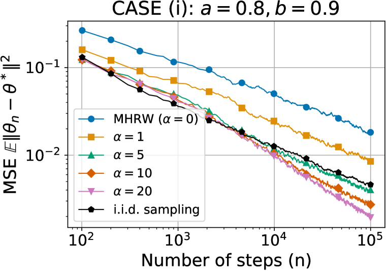
where and are step size sequences decreasing to zero, and is the SRRW kernel in (3). Current non-asymptotic analyses require globally Lipschitz mean field function (Chen et al., 2020b; Doan, 2021; Zeng et al., 2021; Even, 2023) and is thus inapplicable to SA-SRRW since the mean field function of the SRRW iterates (4b) is only locally Lipschitz (details deferred to Appendix B). Instead, we successfully obtain non-trivial results by taking an asymptotic CLT-based approach to analyze (4). This goes beyond just analyzing the asymptotic sampling covariance555Sampling covariance corresponds to only the empirical distribution in (4b). as in Doshi et al. (2023), the result therein forming a special case of ours by setting and considering only (4a) and (4b), that is, in the absence of optimization iteration (4c). Specifically, we capture the effect of SRRW’s hyper-parameter on the asymptotic speed of convergence of the optimization error term to zero via explicit deduction of its asymptotic covariance matrix. See Figure 1 for illustration.

Our Contributions.
1. Given any time-reversible ‘base’ Markov chain with transition kernel and stationary distribution , we generalize first and second order convergence results of to target measure (Theorems 4.1 and 4.2 in Doshi et al., 2023) to a class of weighted empirical measures, through the use of more general step sizes . This includes showing that the asymptotic sampling covariance terms decrease to zero at rate , thus quantifying the effect of self-repellent on . Our generalization is not for the sake thereof and is shown in Section 3 to be crucial for the design of step sizes .
2. Building upon the convergence results for iterates , we analyze the algorithm (4) driven by the SRRW kernel in (3) with step sizes and separated into three disjoint cases:
-
(i)
, and we say that is on the slower timescale compared to ;
-
(ii)
, and we say that and are on the same timescale;
-
(iii)
, and we say that is on the faster timescale compared to .
For any and let and refer to the corresponding cases (i), (ii) and (iii), we show that
featuring distinct asymptotic covariance matrices and , respectively. The three matrices coincide when ,666The case is equivalent to simply running the base Markov chain, since from (3) we have , thus bypassing the SRRW’s effect and rendering all three cases nearly the same.. Moreover, the derivation of the CLT for cases (i) and (iii), for which (4) corresponds to two-timescale SA with controlled Markov noise, is the first of its kind and thus a key technical contribution in this paper, as expanded upon in Section 3.
3. For case (i), we show that decreases to zero (in the sense of Loewner ordering introduced in Section 2.1) as increases, with rate . This is especially surprising, since the asymptotic performance benefit from using the SRRW kernel with in (3), to drive the noise terms , is amplified in the context of distributed learning and estimating ; compared to the sampling case, for which the rate is as mentioned earlier. For case (iii), we show that for all , implying that using the SRRW in this case provides no asymptotic benefit than the original base Markov chain, and thus performs worse than case (i). In summary, we deduce that for all and .777In particular, this is the reason why we advocate for a more general step size in the SRRW iterates with , allowing us to choose with to satisfy for case (i).
4. We numerically simulate our SA-SRRW algorithm on various real-world datasets, focusing on a binary classification task, to evaluate its performance across all three cases. By carefully choosing the function in SA-SRRW, we test the SGD and algorithms driven by SRRW. Our findings consistently highlight the superiority of case (i) over cases (ii) and (iii) for diverse values, even in their finite time performance. Notably, our tests validate the variance reduction at a rate of for case (i), suggesting it as the best algorithmic choice among the three cases.
2 Preliminaries and Model Setup
In Section 2.1, we first standardize the notations used throughout the paper, and define key mathematical terms and quantities used in our theoretical analyses. Then, in Section 2.2, we consolidate the model assumptions of our SA-SRRW algorithm (4). We then go on to discuss our assumptions, and provide additional interpretations of our use of generalized step-sizes.
2.1 Basic Notations and Definitions
Vectors are denoted by lower-case bold letters, e.g., , and matrices by upper-case bold, e.g., . is the transpose of the matrix inverse . The diagonal matrix is formed by vector with as the ’th diagonal entry. Let and denote vectors of all ones and zeros, respectively. The identity matrix is represented by , with subscripts indicating dimensions as needed. A matrix is Hurwitz if all its eigenvalues possess strictly negative real parts. denotes an indicator function with condition in parentheses. We use to denote both the Euclidean norm of vectors and the spectral norm of matrices. Two symmetric matrices follow Loewner ordering if is positive semi-definite and . This slightly differs from the conventional definition with , which allows .
Throughout the paper, the matrix and vector are used exclusively to denote an -dimensional transition kernel of an ergodic Markov chain, and its stationary distribution, respectively. Without loss of generality, we assume if and only if . Markov chains satisfying the detailed balance equation, where for all , are termed time-reversible. For such chains, we use (resp. ) to denote the ’th left (resp. right) eigenpair where the eigenvalues are ordered: , with and in . We assume eigenvectors to be normalized such that for all , and we have and for all . We direct the reader to Aldous & Fill (2002, Chapter 3.4) for a detailed exposition on spectral properties of time-reversible Markov chains.
2.2 SA-SRRW: Key Assumptions and Discussions
Assumptions: All results in our paper are proved under the following assumptions.
-
(A1)
The function , is a continuous at every , and there exists a positive constant such that for every .
-
(A2)
Step sizes and follow , and , where .
-
(A3)
Roots of function are disjoint, which comprise the globally attracting set of the associated ordinary differential equation (ODE) for iteration (4c), given by .
-
(A4)
For any , the iterate sequence (resp. ) is -almost surely contained within a compact subset of (resp. ).
Discussions on Assumptions: Assumption A1 requires to only be locally Lipschitz albeit with linear growth, and is less stringent than the globally Lipschitz assumption prevalent in optimization literature (Li & Wai, 2022; Hendrikx, 2023; Even, 2023).
Assumption A2 is the general umbrella assumption under which cases (i), (ii) and (iii) mentioned in Section 1 are extracted by setting: (i) , (ii) , and (iii) . Cases (i) and (iii) render on different timescales; the polynomial form of widely assumed in the two-timescale SA literature (Mokkadem & Pelletier, 2006; Zeng et al., 2021; Hong et al., 2023). Case (ii) characterizes the SA-SRRW algorithm (4) as a single-timescale SA with polynomially decreasing step size, and is among the most common assumptions in the SA literature (Borkar, 2022; Fort, 2015; Li et al., 2023). In all three cases, the form of ensures such that the SRRW iterates in (4b) is within , ensuring that is well-defined for all .
In Assumption A3, limiting dynamics of SA iterations closely follow trajectories of their associated ODE, and assuming the existence of globally stable equilibria is standard (Borkar, 2022; Fort, 2015; Li et al., 2023). In optimization problems, this is equivalent to assuming the existence of at most countably many local minima.
Assumption A4 assumes almost sure boundedness of iterates and , which is a common assumption in SA algorithms (Kushner & Yin, 2003; Chen, 2006; Borkar, 2022; Karmakar & Bhatnagar, 2018; Li et al., 2023) for the stability of the SA iterations by ensuring the well-definiteness of all quantities involved. Stability of the weighted empirical measure of the SRRW process is practically ensured by studying (4b) with a truncation-based procedure (see Doshi et al., 2023, Remark 4.5 and Appendix E for a comprehensive explanation), while that for is usually ensured either as a by-product of the algorithm design, or via mechanisms such as projections onto a compact subset of , depending on the application context.
We now provide additional discussions regarding the step-size assumptions and their implications on the SRRW iteration (4b).
SRRW with General Step Size: As shown in Benaim & Cloez (2015, Remark 1.1), albeit for a completely different non-linear Markov kernel driving the algorithm therein, iterates of (4b) can also be expressed as weighted empirical measures of , in the following form:
| (5) |
for all . For the special case when as in Doshi et al. (2023), we have for all and is the typical, unweighted empirical measure. For the additional case considered in our paper, when for as in assumption A2, we can approximate and . This implies that will increase at sub-exponential rate, giving more weight to recent visit counts and allowing it to quickly ‘forget’ the poor initial measure and shed the correlation with the initial choice of . This ‘speed up’ effect by setting is guaranteed in case (i) irrespective of the choice of in Assumption A2, and in Section 3 we show how this can lead to further reduction in covariance of optimization error in the asymptotic regime.
Additional assumption for case (iii): Before moving on to Section 3, we take another look at the case when , and replace A3 with the following, stronger assumption only for case (iii).
-
(A3′)
For any , there exists a function such that for some , and is Hurwitz.
While Assumption A3′ for case (iii) is much stronger than A3, it is not detrimental to the overall results of our paper, since case (i) is of far greater interest as impressed upon in Section 1. This is discussed further in Appendix C.
3 Asymptotic Analysis of the SA-SRRW Algorithm
In this section, we provide the main results for the SA-SRRW algorithm (4). We first present the a.s. convergence and the CLT result for SRRW with generalized step size, extending the results in Doshi et al. (2023). Building upon this, we present the a.s. convergence and the CLT result for the SA iterate under different settings of step sizes. We then shift our focus to the analysis of the different asymptotic covariance matrices emerging out of the CLT result, and capture the effect of and the step sizes, particularly in cases (i) and (iii), on via performance ordering.
Almost Sure convergence and CLT: The following result establishes first and second order convergence of the sequence , which represents the weighted empirical measures of the SRRW process , based on the update rule in (4b).
Lemma 3.1.
Lemma 3.1 shows that the SRRW iterates converges to the target distribution a.s. even under the general step size for . We also observe that the asymptotic covariance matrix decreases at rate . Lemma 3.1 aligns with Doshi et al. (2023, Theorem 4.2 and Corollary 4.3) for the special case of , and is therefore more general. Critically, it helps us establish our next result regarding the first-order convergence for the optimization iterate sequence following update rule (4c), as well as its second-order convergence result, which follows shortly after. The proofs of Lemma 3.1 and our next result, Theorem 3.2, are deferred to Appendix D. In what follows, , and refer to cases (i), (ii), and (iii) in Section 2.2, respectively. All subsequent results are proven under Assumptions A1 to A4, with A3′ replacing A3 only when the step sizes satisfy case (iii).
Theorem 3.2.
For , and any initial , we have as for some , -almost surely.
In the stochastic optimization context, the above result ensures convergence of iterates to a local minimizer . Loosely speaking, the first-order convergence of in Lemma 3.1 as well as that of are closely related to the convergence of trajectories of the (coupled) mean-field ODE, written in a matrix-vector form as
| (7) |
where matrix for any . Here, is the stationary distribution of the SRRW kernel and is shown in Doshi et al. (2023) to be given by . The Jacobian matrix of (7) when evaluated at equilibria for captures the behaviour of solutions of the mean-field in their vicinity, and plays an important role in the asymptotic covariance matrices arising out of our CLT results. We evaluate this Jacobian matrix as a function of to be given by
| (8) |
The derivation of is referred to Appendix E.1.888The Jacobian is – dimensional, with and . Following this, all matrices written in a block form, such as matrix in (9), will inherit the same dimensional structure. Here, is a zero matrix since is devoid of . While matrix is exactly of the form in Doshi et al. (2023, Lemma 3.4) to characterize the SRRW performance, our analysis includes an additional matrix , which captures the effect of on in the ODE (7), which translates to the influence of our generalized SRRW empirical measure on the SA iterates in (4).
For notational simplicity, and without loss of generality, all our remaining results are stated while conditioning on the event that , for some . We also adopt the shorthand notation to represent . Our main CLT result is as follows, with its proof deferred to Appendix E.
Theorem 3.3.
For , SA-SRRW in (4) is a two-timescale SA with controlled Markov noise. While a few works study the CLT of two-timescale SA with the stochastic input being a martingale-difference (i.i.d.) noise (Konda & Tsitsiklis, 2004; Mokkadem & Pelletier, 2006), a CLT result covering the case of controlled Markov noise (e.g., ), a far more general setting than martingale-difference noise, is still an open problem. Thus, we here prove our CLT for from scratch by a series of careful decompositions of the Markovian noise, ultimately into a martingale-difference term and several non-vanishing noise terms through repeated application of the Poisson equation (Benveniste et al., 2012; Fort, 2015). Although the form of the resulting asymptotic covariance looks similar to that for the martingale-difference case in (Konda & Tsitsiklis, 2004; Mokkadem & Pelletier, 2006) at first glance, they are not equivalent. Specifically, captures both the effect of SRRW hyper-parameter , as well as that of the underlying base Markov chain via eigenpairs of its transition probability matrix in matrix , whereas the latter only covers the martingale-difference noise terms as a special case.
When , that is, , algorithm (4) can be regarded as a single-timescale SA algorithm. In this case, we utilize the CLT in Fort (2015, Theorem 2.1) to obtain the implicit form of as shown in Theorem 3.3. However, being non-zero for restricts us from obtaining an explicit form for the covariance term corresponding to SA iterate errors . On the other hand, for , the nature of two-timescale structure causes and to become asymptotically independent with zero correlation terms inside in (10), and we can explicitly deduce . We now take a deeper dive into and study its effect on .
Covariance Ordering of SA-SRRW: We refer the reader to Appendix F for proofs of all remaining results. We begin by focusing on case (i) and capturing the impact of on .
Proposition 3.4.
For all , we have . Furthermore, decreases to zero at a rate of .
Proposition 3.4 proves a monotonic reduction (in terms of Loewner ordering) of as increases. Moreover, the decrease rate surpasses the rate seen in and the sampling application in Doshi et al. (2023, Corollary 4.7), and is also empirically observed in our simulation in Section 4.999Further insights of are tied to the two-timescale structure, particularly in case (i), which places on the slow timescale so that the correlation terms in the Jacobian matrix in (8) come into play. Technical details are referred to Appendix E.2, where we show the form of . Suppose we consider the same SA now driven by an i.i.d. sequence with the same marginal distribution . Then, our Proposition 3.4 asserts that a token algorithm employing SRRW (walk on a graph) with large enough on a general graph can actually produce better SA iterates with its asymptotic covariance going down to zero, than a ‘hypothetical situation’ where the walker is able to access any node with probability from anywhere in one step (more like a random jumper). This can be seen by noting that for large time , the scaled MSE is composed of the diagonal entries of the covariance matrix , which, as we discuss in detail in Appendix F.2, are decreasing in as a consequence of the Loewner ordering in Proposition 3.4. For large enough , the scaled MSE for SA-SRRW becomes smaller than its i.i.d. counterpart, which is always a constant. Although Doshi et al. (2023) alluded this for sampling applications with , we broaden its horizons to distributed optimization problem with using tokens on graphs. Our subsequent result concerns the performance comparison between cases (i) and (iii).
Corollary 3.5.
For any , we have .
4 Simulation
In this section, we simulate our SA-SRRW algorithm on the wikiVote graph (Leskovec & Krevl, 2014), comprising nodes and edges. We configure the SRRW’s base Markov chain as the MHRW with a uniform target distribution . For distributed optimization, we consider the following regularized binary classification problem:
| (12) |
where is the ijcnn1 dataset (with features, i.e., ) from LIBSVM (Chang & Lin, 2011), and penalty parameter . Each node in the wikiVote graph is assigned one data point, thus data points in total. We perform SRRW driven SGD (SGD-SRRW) and SRRW driven stochastic heavy ball (SHB-SRRW) algorithms (see (13) in Appendix A for its algorithm). We fix the step size for the SA iterates and adjust in the SRRW iterates to cover all three cases discussed in this paper: (i) ; (ii) ; (iii) . We use mean square error (MSE), i.e., , to measure the error on the SA iterates.
Our results are presented in Figures 2 and 3, where each experiment is repeated times. Figures 2(a) and 2(b), based on wikiVote graph, highlight the consistent performance ordering across different values for both algorithms over almost all time (not just asymptotically). Notably, curves for outperform that of the i.i.d. sampling (in black) even under the graph constraints. Figure 2(c) on the smaller Dolphins graph (Rossi & Ahmed, 2015) - nodes and edges - illustrates that the points of (, MSE) pair arising from SGD-SRRW at time align with a curve in the form of to showcase rates. This smaller graph allows for longer simulations to observe the asymptotic behaviour. Additionally, among the three cases examined at identical values, Figures 3(a) - 3(c) confirm that case (i) performs consistently better than the rest, underscoring its superiority in practice. Further results, including those from non-convex functions and additional datasets, are deferred to Appendix H due to space constraints.


5 Conclusion
In this paper, we show both theoretically and empirically that the SRRW as a drop-in replacement for Markov chains can provide significant performance improvements when used for token algorithms, where the acceleration comes purely from the careful analysis of the stochastic input of the algorithm, without changing the optimization iteration itself. Our paper is an instance where the asymptotic analysis approach allows the design of better algorithms despite the usage of unconventional noise sequences such as nonlinear Markov chains like the SRRW, for which traditional finite-time analytical approaches fall short, thus advocating their wider adoption.
References
- Aldous & Fill (2002) David Aldous and James Allen Fill. Reversible markov chains and random walks on graphs, 2002. Unfinished monograph, recompiled 2014, available at http://www.stat.berkeley.edu/~aldous/RWG/book.html.
- Andrieu et al. (2007) Christophe Andrieu, Ajay Jasra, Arnaud Doucet, and Pierre Del Moral. Non-linear markov chain monte carlo. In Esaim: Proceedings, volume 19, pp. 79–84. EDP Sciences, 2007.
- Ayache & El Rouayheb (2021) Ghadir Ayache and Salim El Rouayheb. Private weighted random walk stochastic gradient descent. IEEE Journal on Selected Areas in Information Theory, 2(1):452–463, 2021.
- Barakat & Bianchi (2021) Anas Barakat and Pascal Bianchi. Convergence and dynamical behavior of the adam algorithm for nonconvex stochastic optimization. SIAM Journal on Optimization, 31(1):244–274, 2021.
- Barakat et al. (2021) Anas Barakat, Pascal Bianchi, Walid Hachem, and Sholom Schechtman. Stochastic optimization with momentum: convergence, fluctuations, and traps avoidance. Electronic Journal of Statistics, 15(2):3892–3947, 2021.
- Benaim & Cloez (2015) M Benaim and Bertrand Cloez. A stochastic approximation approach to quasi-stationary distributions on finite spaces. Electronic Communications in Probability 37 (20), 1-14.(2015), 2015.
- Benveniste et al. (2012) Albert Benveniste, Michel Métivier, and Pierre Priouret. Adaptive algorithms and stochastic approximations, volume 22. Springer Science & Business Media, 2012.
- Borkar (2022) V.S. Borkar. Stochastic Approximation: A Dynamical Systems Viewpoint: Second Edition. Texts and Readings in Mathematics. Hindustan Book Agency, 2022. ISBN 9788195196111.
- Bottou et al. (2018) Léon Bottou, Frank E Curtis, and Jorge Nocedal. Optimization methods for large-scale machine learning. SIAM review, 60(2):223–311, 2018.
- Boyd et al. (2006) Stephen Boyd, Arpita Ghosh, Balaji Prabhakar, and Devavrat Shah. Randomized gossip algorithms. IEEE transactions on information theory, 52(6):2508–2530, 2006.
- Brémaud (2013) Pierre Brémaud. Markov chains: Gibbs fields, Monte Carlo simulation, and queues, volume 31. Springer Science & Business Media, 2013.
- Chang & Lin (2011) Chih-Chung Chang and Chih-Jen Lin. Libsvm: a library for support vector machines. ACM transactions on intelligent systems and technology (TIST), 2(3):1–27, 2011.
- Chellaboina & Haddad (2008) VijaySekhar Chellaboina and Wassim M Haddad. Nonlinear dynamical systems and control: A Lyapunov-based approach. Princeton University Press, 2008.
- Chellapandi et al. (2023) Vishnu Pandi Chellapandi, Antesh Upadhyay, Abolfazl Hashemi, and Stanislaw H Zak. On the convergence of decentralized federated learning under imperfect information sharing. arXiv preprint arXiv:2303.10695, 2023.
- Chen (2006) Han-Fu Chen. Stochastic approximation and its applications, volume 64. Springer Science & Business Media, 2006.
- Chen et al. (2020a) Shuhang Chen, Adithya Devraj, Ana Busic, and Sean Meyn. Explicit mean-square error bounds for monte-carlo and linear stochastic approximation. In International Conference on Artificial Intelligence and Statistics, pp. 4173–4183. PMLR, 2020a.
- Chen et al. (2020b) Zaiwei Chen, Siva Theja Maguluri, Sanjay Shakkottai, and Karthikeyan Shanmugam. Finite-sample analysis of stochastic approximation using smooth convex envelopes. arXiv preprint arXiv:2002.00874, 2020b.
- Chen et al. (2022) Zaiwei Chen, Sheng Zhang, Thinh T Doan, John-Paul Clarke, and Siva Theja Maguluri. Finite-sample analysis of nonlinear stochastic approximation with applications in reinforcement learning. Automatica, 146:110623, 2022.
- Davis (1970) Burgess Davis. On the intergrability of the martingale square function. Israel Journal of Mathematics, 8:187–190, 1970.
- Defazio et al. (2014) Aaron Defazio, Francis Bach, and Simon Lacoste-Julien. Saga: a fast incremental gradient method with support for non-strongly convex composite objectives. In Advances in neural information processing systems, volume 1, 2014.
- Del Moral & Doucet (2010) Pierre Del Moral and Arnaud Doucet. Interacting markov chain monte carlo methods for solving nonlinear measure-valued equations1. The Annals of Applied Probability, 20(2):593–639, 2010.
- Del Moral & Miclo (2006) Pierre Del Moral and Laurent Miclo. Self-interacting markov chains. Stochastic Analysis and Applications, 24(3):615–660, 2006.
- Delyon (2000) Bernard Delyon. Stochastic approximation with decreasing gain: Convergence and asymptotic theory. Technical report, Université de Rennes, 2000.
- Delyon et al. (1999) Bernard Delyon, Marc Lavielle, and Eric Moulines. Convergence of a stochastic approximation version of the em algorithm. Annals of statistics, pp. 94–128, 1999.
- Devraj & Meyn (2017) Adithya M Devraj and Sean P Meyn. Zap q-learning. In Proceedings of the 31st International Conference on Neural Information Processing Systems, pp. 2232–2241, 2017.
- Devraj & Meyn (2021) Adithya M. Devraj and Sean P. Meyn. Q-learning with uniformly bounded variance. IEEE Transactions on Automatic Control, 2021.
- Doan et al. (2019) Thinh Doan, Siva Maguluri, and Justin Romberg. Finite-time analysis of distributed td (0) with linear function approximation on multi-agent reinforcement learning. In International Conference on Machine Learning, pp. 1626–1635. PMLR, 2019.
- Doan (2021) Thinh T Doan. Finite-time convergence rates of nonlinear two-time-scale stochastic approximation under markovian noise. arXiv preprint arXiv:2104.01627, 2021.
- Doan et al. (2020) Thinh T Doan, Lam M Nguyen, Nhan H Pham, and Justin Romberg. Convergence rates of accelerated markov gradient descent with applications in reinforcement learning. arXiv preprint arXiv:2002.02873, 2020.
- Doshi et al. (2023) Vishwaraj Doshi, Jie Hu, and Do Young Eun. Self-repellent random walks on general graphs–achieving minimal sampling variance via nonlinear markov chains. In International Conference on Machine Learning. PMLR, 2023.
- Duflo (1996) Marie Duflo. Algorithmes stochastiques, volume 23. Springer, 1996.
- Even (2023) Mathieu Even. Stochastic gradient descent under markovian sampling schemes. In International Conference on Machine Learning, 2023.
- Fort (2015) Gersende Fort. Central limit theorems for stochastic approximation with controlled markov chain dynamics. ESAIM: Probability and Statistics, 19:60–80, 2015.
- Gadat et al. (2018) Sébastien Gadat, Fabien Panloup, and Sofiane Saadane. Stochastic heavy ball. Electronic Journal of Statistics, 12:461–529, 2018.
- Guo et al. (2020) Xin Guo, Jiequn Han, Mahan Tajrobehkar, and Wenpin Tang. Escaping saddle points efficiently with occupation-time-adapted perturbations. arXiv preprint arXiv:2005.04507, 2020.
- Hall et al. (2014) P. Hall, C.C. Heyde, Z.W. Birnbauam, and E. Lukacs. Martingale Limit Theory and Its Application. Communication and Behavior. Elsevier Science, 2014.
- Hendrikx (2023) Hadrien Hendrikx. A principled framework for the design and analysis of token algorithms. In International Conference on Artificial Intelligence and Statistics, pp. 470–489. PMLR, 2023.
- Hong et al. (2023) Mingyi Hong, Hoi-To Wai, Zhaoran Wang, and Zhuoran Yang. A two-timescale stochastic algorithm framework for bilevel optimization: Complexity analysis and application to actor-critic. SIAM Journal on Optimization, 33(1):147–180, 2023.
- Hu et al. (2022) Jie Hu, Vishwaraj Doshi, and Do Young Eun. Efficiency ordering of stochastic gradient descent. In Advances in Neural Information Processing Systems, 2022.
- Jin et al. (2017) Chi Jin, Rong Ge, Praneeth Netrapalli, Sham M Kakade, and Michael I Jordan. How to escape saddle points efficiently. In International conference on machine learning, pp. 1724–1732. PMLR, 2017.
- Jin et al. (2018) Chi Jin, Praneeth Netrapalli, and Michael I Jordan. Accelerated gradient descent escapes saddle points faster than gradient descent. In Conference On Learning Theory, pp. 1042–1085. PMLR, 2018.
- Jin et al. (2021) Chi Jin, Praneeth Netrapalli, Rong Ge, Sham M Kakade, and Michael I Jordan. On nonconvex optimization for machine learning: Gradients, stochasticity, and saddle points. Journal of the ACM (JACM), 68(2):1–29, 2021.
- Karimi et al. (2019) Belhal Karimi, Blazej Miasojedow, Eric Moulines, and Hoi-To Wai. Non-asymptotic analysis of biased stochastic approximation scheme. In Conference on Learning Theory, pp. 1944–1974. PMLR, 2019.
- Karmakar & Bhatnagar (2018) Prasenjit Karmakar and Shalabh Bhatnagar. Two time-scale stochastic approximation with controlled markov noise and off-policy temporal-difference learning. Mathematics of Operations Research, 43(1):130–151, 2018.
- Khaled & Richtárik (2023) Ahmed Khaled and Peter Richtárik. Better theory for SGD in the nonconvex world. Transactions on Machine Learning Research, 2023. ISSN 2835-8856.
- Kingma & Ba (2015) Diederik P. Kingma and Jimmy Ba. Adam: A method for stochastic optimization. In ICLR, 2015.
- Konda & Tsitsiklis (2004) Vijay R Konda and John N Tsitsiklis. Convergence rate of linear two-time-scale stochastic approximation. The Annals of Applied Probability, 14(2):796–819, 2004.
- Kushner & Yin (2003) Harold Kushner and G George Yin. Stochastic approximation and recursive algorithms and applications, volume 35. Springer Science & Business Media, 2003.
- Lalitha et al. (2018) Anusha Lalitha, Shubhanshu Shekhar, Tara Javidi, and Farinaz Koushanfar. Fully decentralized federated learning. In Advances in neural information processing systems, 2018.
- Leskovec & Krevl (2014) Jure Leskovec and Andrej Krevl. Snap datasets: Stanford large network dataset collection, 2014.
- Levin & Peres (2017) David A Levin and Yuval Peres. Markov chains and mixing times, volume 107. American Mathematical Soc., 2017.
- Li & Wai (2022) Qiang Li and Hoi-To Wai. State dependent performative prediction with stochastic approximation. In International Conference on Artificial Intelligence and Statistics, pp. 3164–3186. PMLR, 2022.
- Li et al. (2022) Tiejun Li, Tiannan Xiao, and Guoguo Yang. Revisiting the central limit theorems for the sgd-type methods. arXiv preprint arXiv:2207.11755, 2022.
- Li et al. (2023) Xiang Li, Jiadong Liang, and Zhihua Zhang. Online statistical inference for nonlinear stochastic approximation with markovian data. arXiv preprint arXiv:2302.07690, 2023.
- McMahan et al. (2017) Brendan McMahan, Eider Moore, Daniel Ramage, Seth Hampson, and Blaise Aguera y Arcas. Communication-efficient learning of deep networks from decentralized data. In Artificial intelligence and statistics, pp. 1273–1282. PMLR, 2017.
- Meyn (2022) Sean Meyn. Control systems and reinforcement learning. Cambridge University Press, 2022.
- Mokkadem & Pelletier (2005) Abdelkader Mokkadem and Mariane Pelletier. The compact law of the iterated logarithm for multivariate stochastic approximation algorithms. Stochastic analysis and applications, 23(1):181–203, 2005.
- Mokkadem & Pelletier (2006) Abdelkader Mokkadem and Mariane Pelletier. Convergence rate and averaging of nonlinear two-time-scale stochastic approximation algorithms. Annals of Applied Probability, 16(3):1671–1702, 2006.
- Morral et al. (2017) Gemma Morral, Pascal Bianchi, and Gersende Fort. Success and failure of adaptation-diffusion algorithms with decaying step size in multiagent networks. IEEE Transactions on Signal Processing, 65(11):2798–2813, 2017.
- Mou et al. (2020) Wenlong Mou, Chris Junchi Li, Martin J Wainwright, Peter L Bartlett, and Michael I Jordan. On linear stochastic approximation: Fine-grained polyak-ruppert and non-asymptotic concentration. In Conference on Learning Theory, pp. 2947–2997. PMLR, 2020.
- Nedic (2020) Angelia Nedic. Distributed gradient methods for convex machine learning problems in networks: Distributed optimization. IEEE Signal Processing Magazine, 37(3):92–101, 2020.
- Olshevsky (2022) Alex Olshevsky. Asymptotic network independence and step-size for a distributed subgradient method. Journal of Machine Learning Research, 23(69):1–32, 2022.
- Pelletier (1998) Mariane Pelletier. On the almost sure asymptotic behaviour of stochastic algorithms. Stochastic processes and their applications, 78(2):217–244, 1998.
- Reddi et al. (2018) Sashank J. Reddi, Satyen Kale, and Sanjiv Kumar. On the convergence of adam and beyond. In International Conference on Learning Representations, 2018.
- Rossi & Ahmed (2015) Ryan A. Rossi and Nesreen K. Ahmed. The network data repository with interactive graph analytics and visualization. In AAAI, 2015.
- Schmidt et al. (2017) Mark Schmidt, Nicolas Le Roux, and Francis Bach. Minimizing finite sums with the stochastic average gradient. Mathematical Programming, 162:83–112, 2017.
- Sun et al. (2018) Tao Sun, Yuejiao Sun, and Wotao Yin. On markov chain gradient descent. In Advances in neural information processing systems, volume 31, 2018.
- Triastcyn et al. (2022) Aleksei Triastcyn, Matthias Reisser, and Christos Louizos. Decentralized learning with random walks and communication-efficient adaptive optimization. In Workshop on Federated Learning: Recent Advances and New Challenges (in Conjunction with NeurIPS 2022), 2022.
- Vogels et al. (2021) Thijs Vogels, Lie He, Anastasiia Koloskova, Sai Praneeth Karimireddy, Tao Lin, Sebastian U Stich, and Martin Jaggi. Relaysum for decentralized deep learning on heterogeneous data. In Advances in Neural Information Processing Systems, volume 34, pp. 28004–28015, 2021.
- Wang et al. (2019) Jianyu Wang, Anit Kumar Sahu, Zhouyi Yang, Gauri Joshi, and Soummya Kar. Matcha: Speeding up decentralized sgd via matching decomposition sampling. In 2019 Sixth Indian Control Conference (ICC), pp. 299–300. IEEE, 2019.
- Yaji & Bhatnagar (2020) Vinayaka G Yaji and Shalabh Bhatnagar. Stochastic recursive inclusions in two timescales with nonadditive iterate-dependent markov noise. Mathematics of Operations Research, 45(4):1405–1444, 2020.
- Ye et al. (2022) Hao Ye, Le Liang, and Geoffrey Ye Li. Decentralized federated learning with unreliable communications. IEEE Journal of Selected Topics in Signal Processing, 16(3):487–500, 2022.
- Zeng et al. (2021) Sihan Zeng, Thinh T Doan, and Justin Romberg. A two-time-scale stochastic optimization framework with applications in control and reinforcement learning. arXiv preprint arXiv:2109.14756, 2021.
Appendix A Examples of Stochastic Algorithms of the form (2).
In the literature of stochastic optimizations, many SGD variants have been proposed by introducing an auxiliary variable to improve convergence. In what follows, we present two SGD variants with decreasing step size that can be presented in the form of (2): SHB (Gadat et al., 2018; Li et al., 2022) and momentum-based algorithm (Barakat et al., 2021; Barakat & Bianchi, 2021).
| (13) |
where , , and the square and square root in (13) (b) are element-wise operators.101010For ease of expression, we simplify the original SHB and momentum-based algorithms from Gadat et al. (2018); Li et al. (2022); Barakat et al. (2021); Barakat & Bianchi (2021), setting all tunable parameters to and resulting in (13).
For SHB, we introduce an augmented variable and function defined as follows:
For the general momentum-based algorithm, we define
Thus, we can reformulate both algorithms in (13) as . This augmentation approach was previously adopted in (Gadat et al., 2018; Barakat et al., 2021; Barakat & Bianchi, 2021; Li et al., 2022) to analyze the asymptotic performance of algorithms in (13) using an i.i.d. sequence . Consequently, the general SA iteration (2) includes these SGD variants. However, we mainly focus on the CLT for the general SA driven by SRRW in this paper. Pursuing the explicit CLT results of these SGD variants with specific form of function driven by the SRRW sequence is out of the scope of this paper.
Appendix B Discussion on Mean Field Function of SRRW Iterates (4b)
Non-asymptotic analyses have seen extensive attention recently in both single-timescale SA literature (Sun et al., 2018; Karimi et al., 2019; Chen et al., 2020b; 2022) and two-timescale SA literature (Doan, 2021; Zeng et al., 2021). Specifically, single-timescale SA has the following form:
and function is the mean field of function . Similarly, for two-timescale SA, we have the following recursions:
where and are on different timescales, and function is the mean field of function for . All the aforementioned works require the mean field function in the single-timescale SA (or in the two-timescale SA) to be globally Lipschitz with a Lipschitz constant to proceed with the derivation of finite-time bounds including the constant .
Here, we show that the mean field function in the SRRW iterates (4b) is not globally Lipschitz, where is the stationary distribution of the SRRW kernel defined in (3). To this end, we show that each entry of Jacobian matrix of goes unbounded because a multivariate function is Lipschitz if and only if it has bounded partial derivatives. Note that from Doshi et al. (2023, Proposition 2.1), for the -th entry of , we have
| (16) |
Then, the Jacobian matrix of the mean field function , which has been derived in Doshi et al. (2023, Proof of Lemma 3.4 in Appendix B), is given as follows:
| (17) |
for , and
| (18) |
for . Since the empirical distribution , we have for all . For fixed , assume and as they approach zero, the terms , dominate the fraction in (17) and both the numerator and the denominator of the fraction have the same order in terms of . Thus, we have
such that the -th entry of the Jacobian matrix can go unbounded as . Consequently, is not globally Lipschitz for .
Appendix C Discussion on Assumption A3′
When , iterates has smaller step size compared to , thus converges ‘slower’ than . From Assumption A3′, will intuitively converge to some point with the current value from the iteration , i.e., , while the Hurwitz condition is to ensure the stability around . We can see that Assumption A3 is less stringent than A3′ in that it only assumes such condition when such that rather than for all .
One special instance of Assumption A3′ is by assuming the linear SA, e.g., . In this case, is equivalent to . Under the condition that for every , matrix is invertible, we then have
However, this condition is quite strict. Loosely speaking, being invertible for any is similar to saying that any convex combination of is invertible. For example, if we assume are negative definite and they all share the same eigenbasis , e.g., and for all . Then, is invertible.
Another example for Assumption A3′ is when for all , which implies that each agent in the distributed learning has the same local dataset to collaboratively train the model. In this example, such that
Appendix D Proof of Lemma 3.1 and Lemma 3.2
In this section, we demonstrate the almost sure convergence of both and together. This proof naturally incorporates the almost certain convergence of the SRRW iteration in Lemma 3.1, since is independent of (as indicated in (4)), allowing us to separate out its asymptotic results. The same reason applies to the CLT analysis of SRRW iterates and we refer the reader to Section E.1 for the CLT result of in Lemma 3.1.
We will use different techniques for different settings of step sizes in Assumption A2. Specifically, for step sizes , we consider the following scenarios:
- Scenario 1:
-
We consider case(ii): , and will apply the almost sure convergence result of the single-timescale stochastic approximation in Theorem G.8 and verify all the conditions therein.
- Scenario 2:
-
We consider both case(i): and case (iii): . In these two cases, step sizes decrease at different rates, thereby putting iterates on different timescales and resulting in a two-timescale structure. We will apply the existing almost sure convergence result of the two-timescale stochastic approximation with iterate-dependent Markov chain in Yaji & Bhatnagar (2020, Theorem 4) where our SA-SRRW algorithm can be regarded as a special instance.111111However, Yaji & Bhatnagar (2020) paper only analysed the almost sure convergence. The central limit theorem analysis remains unknown in the literature for the two-timescale stochastic approximation with iterate-dependent Markov chains. Thus, our CLT analysis in Section E for this two-timescale structure with iterate-dependent Markov chain is still novel and recognized as our contribution.
D.1 Scenario 1
In Scenario 1, we have . First, we rewrite (4) as
| (19) |
By augmentations, we define the variable and the function . In addition, we define a new Markov chain in the same state space as SRRW sequence . With slight abuse of notation, the transition kernel of is denoted by and its stationary distribution , where and are the transition kernel and its corresponding stationary distribution of SRRW, with of the form
| (20) |
Recall that is the fixed point, i.e., , and is the base Markov chain inside SRRW (see (3)). Then, the mean field
and for in Assumption A3 is the root of , i.e., . The augmented iteration (19) becomes
| (21) |
with the goal of solving . Therefore, we can treat (21) as an SA algorithm driven by a Markov chain with its kernel and stationary distribution , which has been widely studied in the literature (e.g., Delyon (2000); Benveniste et al. (2012); Fort (2015); Li et al. (2023)). In what follows, we demonstrate that for any initial point , the SRRW iteration will almost surely converge to the target distribution , and the SA iteration will almost surely converge to the set .
Now we verify conditions C1 - C4 in Theorem G.8. Our assumption A4 is equivalent to condition C1 and assumption A2 corresponds to condition C2. For condition C3, we set , and the set , including disjoint points. For condition C4, since , or equivalently , is ergodic and time-reversible for a given , as shown in the SRRW work Doshi et al. (2023), it automatically ensures a solution to the Poisson equation, which has been well discussed in Chen et al. (2020a, Section 2) and Benveniste et al. (2012); Meyn (2022). To show (97) and (98) in condition C4, for each given and any , we need to give the explicit solution to the Poisson equation in (96). The notation is defined as follows.
Let . We use to denote the -th column of matrix . Then, we let such that
| (22) |
In addition,
| (23) |
We can check that the form in (22) is indeed the solution of the above Poisson equation. Now, by induction, we get for and for , . Then,
| (24) |
Here, is well defined because is ergodic and time-reversible for any given (proved in Doshi et al. (2023, Appendix A)). Now that both functions and are bounded for each compact subset of by our assumption A1, function is also bounded within the compact subset of its domain. Thus, function is bounded, and (97) is verified. Moreover, for a fixed ,
and this vector-valued function is continuous in because are continuous. We then rewrite (24) as
With continuous functions , we have continuous with respect to , so does . This implies that functions and are locally Lipschitz, which satisfies (98) with for some constant that depends on the compact set . Therefore, condition C4 is checked, and we can apply Theorem G.8 to show the almost convergence result of (19), i.e., almost surely,
Therefore, the almost sure convergence of in Lemma 3.1 is also proved. This finishes the proof in Scenario 1.
D.2 Scenario 2
Now in this subsection, we consider the steps sizes with and . We will frequently use assumptions (B1) - (B5) in Section G.3 and Theorem G.10 to prove the almost sure convergence.
D.2.1 Case (i):
In case (i), is on the slow timescale and is on the fast timescale because iteration has smaller step size than , making converge slower than . Here, we consider the two-timescale SA of the form:
| (25) | |||
Now, we verify assumptions (B1) - (B5) listed in Section G.3.
- •
-
•
Our assumption A3 shows that the function is continuous and differentiable w.r.t and grows linearly with . In addition, also satisfies this property. Therefore, (B2) is satisfied.
-
•
Now that the function is independent of , we can set for any such that from Doshi et al. (2023, Proposition 3.1), and
from Doshi et al. (2023, Lemma 3.4), which is Hurwitz. Furthermore, inherently satisfies the condition for any . Thus, conditions (i) - (iii) in (B3) are satisfied. Additionally, such that for defined in assumption A3, , and is Hurwitz. Therefore, (B3) is checked.
-
•
Assumption (B4) is verified by the nature of SRRW, i.e., its transition kernel and the corresponding stationary distribution with .
Consequently, assumptions (B1) - (B5) are satisfied by our assumptoins A1 - A4 and by Theorem G.10, we have and almost surely.
Next, we consider . As discussed before, (B1), (B2), (B4) and (B5) are satisfied by our assumptions A1 - A4 and the properties of SRRW. The only difference for this step size setting, compared to the previous one , is that the roles of are now flipped, that is, is now on the fast timescale while is on the slow timescale. By a much stronger Assumption A3′, for any , (i) ; (ii) is Hurwitz; (iii) . Hence, conditions (i) - (iii) in (B3) are satisfied. Moreover, we have , being Hurwitz, as mentioned in the previous part. Therefore, (B3) is verified. Accordingly, (B1) - (B5) are checked by our assumptions A1, A2, A3′, A4. By Theorem G.10, we have and almost surely.
Appendix E Proof of Theorem 3.3
This section is devoted to the proof of Theorem 3.3, which also includes the proof of the CLT results for the SRRW iteration in Lemma 3.1. We will use different techniques depending on the step sizes in Assumption A2. Specifically, for step sizes , we will consider three cases: case (i): ; case (ii): ; and case (iii): . For case (ii), we will use the existing CLT result for single-timescale SA in Theorem G.9. For cases (i) and (iii), we will construct our own CLT analysis for the two-timescale structure. We start with case (ii).
E.1 Case (ii):
In this part, we stick to the notations for single-timescale SA studied in Section D.1. To utilize Theorem G.9, apart from Conditions C1 - C4 that have been checked in Section D.1, we still need to check conditions C5 and C6 listed in Section G.2.
Assumption A3 corresponds to condition C5. For condition C6, we need to obtain the explicit form of function to the Poisson equation defined in (96), that is,
where
Following the similar steps in the derivation of from (22) to (24), we have
We also know that and are continuous in for any . For any in a compact set , and are bounded because function is bounded. Therefore, C6 is checked. By Theorem G.9, assume converges to a point for , we have
| (26) |
where is the solution of the following Lyapunov equation
| (27) |
and .
By algebraic calculations of derivative of with respect to in (20),121212One may refer to Doshi et al. (2023, Appendix B, Proof of Lemma 3.4) for the computation of . we can rewrite in terms of , i.e.,
where matrix . Then, we further clarify the matrix . Note that
| (28) |
where the first equality holds because from the definition of SRRW kernel (3), the second equality stems from , and the last term is a conditional expectation over the base Markov chain (with transition kernel ) conditioned on . Similarly, with in the form of (23), we have
From the form ‘’ inside the matrix , the Markov chain is in its stationary regime from the beginning, i.e., for any . Hence,
| (29) |
where the covariance between and for the Markov chain in the stationary regime is . By Brémaud (2013, Theorem 6.3.7), it is demonstrated that is the sampling covariance of the base Markov chain for the test function . Moreover, Brémaud (2013, equation (6.34)) states that this sampling covariance can be rewritten in the following form:
| (30) |
where is the eigenpair of the transition kernel of the ergodic and time-reversible base Markov chain. This completes the proof of case 1.
Remark E.1.
For the CLT result (26), we can look further into the asymptotic covariance matrix as in (27). For convenience, we denote and in the form of (30) such that
| (31) |
For the SRRW iteration , from (26) we know that . Thus, in this remark, we want to obtain the closed form of . By algebraic computations of the bottom-right sub-block matrix, we have
By using result of the closed form solution to the Lyapunov equation (e.g., Lemma G.1) and the eigendecomposition of , we have
| (32) |
E.2 Case (i):
In this part, we mainly focus on the CLT of the SA iteration because the SRRW iteration is independent of and its CLT result has been shown in Remark E.1.
E.2.1 Decomposition of SA-SRRW iteration (4)
We slightly abuse the math notation and define the function
such that . Then, we reformulate (25) as
| (33a) | |||
| (33b) |
There exist functions satisfying the following Poisson equations
| (34a) | |||
| (34b) |
for any and , where , . The existence and explicit form of the solutions , which are continuous w.r.t , follow the similar steps that can be found in Section D.1 from (22) to (24). Thus, we can further decompose (33) into
| (35a) | |||
| (35b) |
such that
| (36a) | |||
| (36b) |
We can observe that (36) differs from the expression in Konda & Tsitsiklis (2004); Mokkadem & Pelletier (2006), which studied the two-timescale SA with Martingale difference noise. Here, due to the presence of the iterate-dependent Markovian noise and the application of the Poisson equation technique, we have additional non-vanishing terms , which will be further examined in Lemma E.2. Additionally, when we apply the Poisson equation to the Martingale difference terms , , we find that there are some covariances that are also non-vanishing as in Lemma E.1. We will mention this again when we obtain those covariances. These extra non-zero noise terms make our analysis distinct from the previous ones since the key assumption (A4) in Mokkadem & Pelletier (2006) is not satisfied. We demonstrate that the long-term average performance of these terms can be managed so that they do not affect the final CLT result.
Analysis of Terms
Consider the filtration , it is evident that are Martingale difference sequences adapted to . Then, we have
| (37) |
Similarly, we have
| (38) |
and
We now focus on . Denote by
| (39) |
and let its expectation w.r.t the stationary distribution be , we can construct another Poisson equation, i.e.,
for some matrix-valued function . Since and are continuous in , functions are also continuous in . Then, we can decompose (39) into
| (40) |
Thus, we have
| (41) |
where .
Following the similar steps above, we can decompose and as
| (42a) | |||
| (42b) |
where and . Here, we note that matrices for are in presence of the current CLT analysis of the two-timescale SA with Martingale difference noise. In addition, , and inherently include the information of the underlying Markov chain (with its eigenpair ()), which is an extension of the previous works (Konda & Tsitsiklis, 2004; Mokkadem & Pelletier, 2006).
Proof.
We now provide the properties of the four terms inside (41) as an example. Note that
We can see that it has exactly the same structure as matrix in (27). Following the similar steps in deducing the explicit form of from (28) to (30), we get
| (44) |
By the almost sure convergence result in Lemma 3.1, a.s. such that a.s.
We next prove that and .
Since is a Martingale difference sequence adapted to , with the Burkholder inequality in Lemma G.2 and , we show that
| (45) |
By assumption A4, is always within some compact set such that and for a given trajectory of ,
| (46) |
and the last term decreases to zero in since .
For , we use Abel transformation and obtain
Since is continuous in , for within a compact set (assumption A4), it is local Lipschitz with a constant such that
where the last inequality arises from (4b), i.e., and because . Also, are upper-bounded by some positive constant . This implies that
Note that
| (47) |
where the last inequality is from . We observe that the last term in (47) is decreasing to zero in because .
Note that , by triangular inequality we have
| (48) |
where the second inequality comes from (45). By (46) and (47) we know that both terms in the last line of (48) are uniformly bounded by constants over time that depend on the set . Therefore, by dominated convergence theorem, taking the limit over the last line of (48) gives
Therefore, we have
We can apply the same steps as above for the other two terms in (42) and obtain the results. ∎
Analysis of Terms
Lemma E.2.
For defined in (35), we have the following results:
| (49a) | |||
| (49b) |
Proof.
For , note that
| (50) |
where the second last inequality is because is continuous in , which stems from continuous functions and . The last inequality is from update rules (4) and for some compact subset by assumption A4. Then, we have because of by assumption A2.
We let such that . Note that , and by assumption A4, is upper bounded by a constant dependent on the compact set, which leads to
Similarly, we can also obtain and . ∎
E.2.2 Effect of SRRW Iteration on SA Iteration
In view of the almost sure convergence results in Lemma 3.1 and Lemma 3.2, for large enough so that both iterations are close to the equilibrium , we can apply the Taylor expansion to functions and in (36) at the point , which results in
| (51a) | |||
| (51b) |
With matrix , we have the following:
| (52) |
Then, (36) becomes
| (53a) | |||
| (53b) |
where and .
Then, inspired by Mokkadem & Pelletier (2006), we decompose iterates and into and . Rewriting (53b) gives
and substituting the above equation back in (53a) gives
| (54) |
From (54) we can see the iteration implicitly embeds the recursions of three sequences
-
•
;
-
•
;
-
•
.
Let and . Below we define two iterations:
| (55a) | |||
| (55b) |
and a remaining term .
Similarly, for iteration , define the sequence such that
| (56) |
and a remaining term
| (57) |
The decomposition of and in the above form is also standard in the single-timescale SA literature (Delyon, 2000; Fort, 2015).
Characterization of Sequences and
we set a Martingale such that
Then, the Martingale difference array becomes
and
where, in view of decomposition of and in (41) and (42), respectively,
| (58a) | |||
| (58b) | |||
| (58c) |
We further decompose into three parts:
| (59) |
Here, we define . By (52) and (43a) in Lemma E.1, we have
| (60) |
Then, we have the following lemma.
Lemma E.3.
Proof.
First, from Lemma G.4, we have for some such that
Applying Lemma G.6, together with a.s. in Lemma E.1, gives
We now consider . Set
we can rewrite as
By the Abel transformation, we have
| (62) |
We know from Lemma E.1 that a.s. because . Besides,
for some constant because and . Moreover,
Applying Lemma G.6 again gives
for some constant .
Finally, we provide an existing lemma below.
Lemma E.4 (Mokkadem & Pelletier (2005) Lemma 4).
For a sequence with decreasing step size for , , a positive semi-definite matrix and a Hurwitz matrix , which is given by
we have
where is the solution of the Lyapunov equation
Then, is a direct application of Lemma E.4. ∎
The last step is to show . Note that
where the second equality is from Lemma G.4. Then, we use Lemma G.6 with to obtain
| (63) |
Additionally, since , we have
Then, it follows that . Therefore, we obtain
Now, we turn to verifying the conditions in Theorem G.3. For some , we have
| (64) |
where the last equality comes from Lemma G.6. Since (64) also holds for , we have
Therefore, all the conditions in Theorem G.3 are satisfied and its application then gives
| (65) |
Furthermore, we have the following lemma about the strong convergence rate of and .
Lemma E.5.
| (66a) | |||
| (66b) |
Proof.
This proof follows Pelletier (1998, Lemma 1). We only need the special case of Pelletier (1998, Lemma 1) that fits our scenario; e.g., we let the two types of step sizes therein to be the same. Specifically, we attach the following lemma.
Lemma E.6 (Pelletier (1998) Lemma 1).
Consider a sequence
where , , and is a Martingale difference sequence adapted to the filtration such that, almost surely, and there exists , , such that . Then, almost surely,
| (67) |
where is a constant dependent on .
By assumption A4, the iterates are bounded within a compact subset . Recall the form of defined in (35), it comprises the functions and , which in turn include the function . We know that is bounded for in some compact set . Thus, for any for some compact set , are bounded and we denote by and as their upper bounds, i.e., and . We only need to replace the upper bound in Lemma E.6 by for the sequence (resp. for the sequence ), i.e.,
| (68a) | |||
| (68b) |
such that a.s. and a.s. which completes the proof. ∎
Note that we have and weakly converge to the same Gaussian distribution from Remark E.1 and (65). Then, weakly converges to zero, implying that converges to zero with probability . Therefore, together with being strictly positive, we have
| (69) |
Characterization of Sequences and
We first consider the sequence . We assume a positive real-valued bounded sequence under the same conditions as in Mokkadem & Pelletier (2006, Definition 1), i.e.,
Definition E.1.
In the case , , which also implies .
In the case , there exist and a nondecreasing slowly varying function such that . When , we require function to be bounded. ∎
Since by a.s. convergence result, we can assume that there exists such that . Then, from (55b), we can use the Abel transformation and obtain
where the last term on the RHS can be rewritten as
Using Lemma G.6 on gives . Then, it follows that for some ,
| (70) |
with the application of Lemma G.4 to the second equality.
Then, we shift our focus on . Specifically, we take (54), (55a), and (56) back to , and obtain
| (71) |
where the second equality is by taking the Taylor expansion .
Define and by convention . Then, we rewrite (71) as
| (72) |
From (72), we can indeed decompose into two parts , where
| (73a) | |||
| (73b) |
This term shares the same recursive form as in the sequence defined in Mokkadem & Pelletier (2006, Lemma 6), which is given below.
Lemma E.7 (Mokkadem & Pelletier (2006) Lemma 6).
Since we already have in (69), together with Lemma E.7, we have
where the second equality comes from .
We now focus on . Define a sequence
| (74) |
and we have
where the last equality comes from the Abel transformation. Note that
for some constant , where the last inequality is from Lemma G.4 and for some constant that depends on . Then,
By Lemma E.1, we have a.s. such that by Lemma G.6, it follows that
Therefore, we have
| (75) |
Consequently, almost surely.
Now we are dealing with and its related sequence . Note that by Lemma E.5 and (69), we have almost surely,
| (76) |
Thus, we can set such that in (70) can be written as
and
In view of assumption A2 and , and , there exists a such that almost surely,
Therefore, almost surely. This completes the proof of Scenario 2.
E.3 Case (iii):
For , we can see that the roles of and are flipped, i.e., is now on fast timescale while is on slow timescale.
We still decompose as , where are defined in (56) and (57), respectively. Since is independent of , the results of and remain the same, i.e., almost surely, from Lemma E.5 and from (69). Then, we define sequences and as follows.
| (77a) | |||
| (77b) |
Moreover, the remaining term .
The proof outline is the same as in the previous scenario:
-
•
We first show weakly converges to the distribution ;
-
•
We analyse and to ensure that these two terms decrease faster than the CLT scale , i.e., ;
-
•
With above two steps, we can show that weakly converges to the distribution .
Analysis of
We first focus on and follow similar steps as we did when we analysed in the previous scenario. We set a Martingale such that
Then,
Following the similar steps in (59) to decompose with (42b), we have
| (78) |
Since share similar forms as in Lemma E.3, we follow the same steps as the proof therein, with the application of Lemma E.1. To avoid repetition, we omit the proof and directly give the following lemma.
Lemma E.8.
Note that here we don’t have the term in above lemma, compared to Lemma E.3, because in the case of , such that . Then, applying Lemma G.1 to derive the closed form of gives
Thus, it follows that
Again, we use the Martingale CLT result in Theorem G.3 and have the following result.
Moreover, similar to the tighter upper bound of proved in Lemma E.5, we utilize the tighter upper bound Lemma E.6 in the proof thereof, and obtain .
Analysis of
Next, we turn to the term in (77b). Taking the norm gives the following inequality for some constant by applying Lemma G.4,
Using Lemma G.6 gives
Thus, . Since , , where . Then, there exists some such that . Together with , we have . Therefore, we have
Analysis of
Lastly, let’s focus on the term . We have
where the second equality is from (53a), the third equality stems from the approximation of . Then, we again use the definition and reiterate the above equation as
where and
| (80) |
For , we follow the same steps from (74) to (75), and obtain .
Next, we consider and want to show that . Again, we utilize Mokkadem & Pelletier (2006, Lemma 6) for and adapt the notation here for the case .
Lemma E.9.
Now we need to further analyse and tighten its big O form, starting from , so that we can finally obtain the big O form of . The following steps are borrowed from the ideas in Mokkadem & Pelletier (2006, Section 2.3.2).
By almost sure convergence result , we have a.s. such that we can first set , and . Then, we redefine
and notice that it still satisfies definition E.1. Then, reapplying this form to (81) gives
and by induction we have for all integers ,
Since , there exists such that , and
| (82) |
Then, as suggested in Mokkadem & Pelletier (2006, Section 2.3.2), we can choose , which also satisfies definition E.1. Then,
By induction, this holds for all such that there exists , and . Equivalently, . Therefore, from (82) we have
Together with , we have such that
Thus, we have finished the proof according to the proof outline mentioned at the beginning of this part.
Appendix F Discussion of Covariance Ordering of SA-SRRW
F.1 Proof of Proposition 3.4
For any and any vector , we have
where the first equality is from the form of in Theorem 3.3. Let , with the dependence on variable left implicit. The matrix , given explicitly in (11) positive semi definite, since for all . Thus, the terms inside the integral are non-negative, and it is enough to provide an ordering on with respect to .
For any ,
where the inequality131313The inequality may not be strict when is low rank, however it will always be true for some choice of , since is not a zero matrix. Thus, the ordering derived still follows our definition of in Section 1, footnote 6. is because for all and any . In fact, the ordering is monotone in , and decreases at rate as seen form its form in the equation above. This completes the proof.
F.2 Discussion regarding Proposition 3.4 and MSE ordering
We can use Proposition 3.4 to show that the MSE of SA iterates of (4c) driven by SRRW eventually becomes smaller than that SA iterates when the stochastic noise is driven by an i.i.d. sequence of random variables. The diagonal entries of are obtained by evaluating , where is the ’th standard basis vector.141414-dimensional vector of all zeros except at the ’th position which is . These diagonal entries are the asymptotic variance corresponding to the element-wise iterate errors, and for large enough , we have for all . Thus, the trace of matrix approximates the scaled MSE, that is for large . Since all entries of go to zero as increases, they get smaller than the corresponding term for the SA algorithm with i.i.d. input for large enough , which achieves a constant MSE in the similarly scaled limit, since the asymptotic covariance is not a function of . Moreover, the value of only needs to be moderately large, since the asymptotic covariance terms decrease at rate as shown in Proposition 3.4.
F.3 Proof of Corollary 3.5
We see that for all , because the form of in Theorem 3.3 is independent of . To prove that , it is enough to show that , since from Proposition 3.4. This is easily checked by substituting in 11, for which . Substituting in the respective forms of and in Theorem 3.3, we get equivalence. This completes the proof.
Appendix G Background Theory
G.1 Technical Lemmas
Lemma G.1 (Solution to the Lyapunov Equation).
If all the eigenvalues of matrix have negative real part, then for every positive semi-definite matrix there exists a unique positive semi-definite matrix satisfying the Lyapunov equation . The explicit solution is given as
| (83) |
Chellaboina & Haddad (2008, Theorem 3.16) states that for a positive definite matrix , there exists a positive definite matrix . The reason they focus on the positive definite matrix is that they require the related autonomous ODE system to be asymptotically stable. However, in this paper we don’t need this requirement. The same steps therein can be used to prove Lemma G.1 and show that if is positive semi-definite, then in the form of (83) is unique and also positive semi-definite.
Lemma G.2 (Burkholder Inequality, Davis (1970), Hall et al. (2014) Theorem 2.10).
Given a Martingale difference sequence , for and some positive constant , we have
| (84) |
Theorem G.3 (Martingale CLT, Delyon (2000) Theorem 30).
If a Martingale difference array satisfies the following condition: for some ,
| (85) |
| (86) |
and
| (87) |
then
| (88) |
∎
Lemma G.4 (Duflo (1996) Proposition 3.I.2).
For a Hurwitz matrix , there exist some positive constants such that for any ,
| (89) |
Lemma G.5 (Fort (2015) Lemma 5.8).
For a Hurwitz matrix , denote by , , the largest real part of its eigenvalues. Let a positive sequence such that . Then for any , there exists a positive constant such that for any ,
| (90) |
Lemma G.6 (Fort (2015) Lemma 5.9, Mokkadem & Pelletier (2006) Lemma 10).
Let be a positive sequence such that and . Let be a nonnegative sequence. Then, for , ,
| (91) |
for some constant .
When and define a positive sequence satisfying , we have
| (92) |
Lemma G.7 (Fort (2015) Lemma 5.10).
For any matrices ,
| (93) |
G.2 Asymptotic Results of Single-Timescale SA
Consider the stochastic approximation in the form of
| (94) |
Let be the transition kernel of the underlying Markov chain with stationary distribution such that with domain . Define an operator for any function such that
| (95) |
Assume that
-
C1.
W.p.1, the closure of is a compact subset of .
-
C2.
.
-
C3.
Function is continuous on and there exists a non-negative function and a compact set such that
-
•
for all and if ;
-
•
the set is such that has an empty interior;
-
•
-
C4.
For every , there exists a solution for the following Poisson equation
(96) for any ; for any compact set ,
(97) and there exist a continuous function , such that for any ,
(98) -
C5.
Denote by the largest real part of the eigenvalues of the Jacobian matrix and assume .
-
C6.
For every , there exists a solution for the following Poisson equation
(99) for any , where
(100) For any compact set ,
(101) and there exist , such that for any ,
(102)
G.3 Asymptotic Results of Two-Timescale SA
For the two-timescale SA with iterate-dependent Markov chain, we have the following iterations:
| (106a) | |||
| (106b) |
with the goal of finding the root such that
| (107) |
We present here a simplified version of the assumptions for single-valued functions that are necessary for the almost sure convergence result in Yaji & Bhatnagar (2020, Theorem 4). The original assumptions are intended for more general set-valued functions .
-
(B1)
The step sizes and , where .
-
(B2)
Assume the function is continuous and differentiable with respect to . There exists a positive constant such that for every . The same condition holds for the function as well.
-
(B3)
Assume there exists a function such that the following three properties hold: (i) for some positive constant ; (ii) the ODE has a globally asymptotically stable equilibrium such that . Additionally, let , there exists a set of disjoint roots , which is the set of globally asymptotically stable equilibria of the ODE .
-
(B4)
is an iterate-dependent Markov process in finite state space . For every , , where the transition kernel is continuous in , and the Markov chain generated by is ergodic so that it admits a stationary distribution , and .
-
(B5)
a.s.
Yaji & Bhatnagar (2020) included assumptions A1 - A9 and A11 for the following Theorem G.10. We briefly show the correspondence of our assumptions (B1) - (B5) and theirs: (B1) with A5, (B2) with A1 and A2, (B3) with A9 and A11, (B4) with A3 and A4, and (B5) with A8. Given that our two-timescale SA framework (106) excludes additional noises (setting them to zero), A6 and A7 therein are inherently met.
Appendix H Additional Simulation Results
H.1 Binary Classification on Additional Datasets
In this part, we perform the binary classification task as in Section 4 on additional datasets, i.e., a9a (with features) and splice (with features) from LIBSVM (Chang & Lin, 2011). Figure 4 provides the performance ordering of different values, and we empirically demonstrate that the curves with still outperform the i.i.d. counterpart. Additionally, Figure 5 compare cases (i) - (iii) under both a9a and splice datasets, and case (i) consistently perform the best.


H.2 Non-convex Linear Regression
We further test SGD-SRRW and SHB-SRRW algorithms with a non-convex function to demonstrate the efficiency of our SA-SRRW algorithm beyond the convex setting. In this task, we simulate the following linear regression problem in Khaled & Richtárik (2023) with non-convex regularization
| (108) |
where the loss function and , with the data points from the ijcnn1 dataset of LIBVIM (Chang & Lin, 2011). We still perform the optimization over the wikiVote graph, as done in Section 4.
The numerical results for the non-convex linear regression taks are presented in Figures 6 and 7, where each experiment is repeated times. Figures 6(a) and 6(b) show that the performance ordering across different values is still preserved for both algorithms over almost all time, and curves for outperform that of the i.i.d. sampling (in black) under the graph topological constraints. Additionally, among the three cases examined at identical values, Figures 7(a) - 7(c) confirm that case (i) performs consistently better than the other two cases, implying that case (i) can even become the best choice for non-convex distributed optimization tasks.