Accelerated Stochastic ExtraGradient: Mixing Hessian and Gradient Similarity to Reduce Communication in Distributed and Federated Learning

Empirical risk minimization is a key concept in supervised machine learning (Shalev-Shwartz et al.,, 2010). This paradigm is used to train a wide range of models, such as linear and logistic regression (Tripepi et al.,, 2008), support vector machines (Moguerza and Muñoz,, 2006), tree-based models (Hehn et al.,, 2020), neural networks (Sannakki and Kulkarni,, 2016), and many more. In essence, this is an optimization of the parameters based on the average losses in data. By minimizing the empirical risk, the model aims to generalize well to unseen samples and make accurate predictions. In order to enhance the overall predictive performance and effectively tackle advanced tasks, it is imperative to train on large datasets. By leveraging such ones during the training process, we aim to maximize the generalization capabilities of models and equip them with the robustness and adaptability required to excel in challenging real-world scenarios (Feng et al.,, 2014). The richness and variety of samples in large datasets provides the depth needed to learn complex patterns, relationships, and nuances, enabling them to make accurate and reliable predictions across a wide range of inputs and conditions. As datasets grow in size and complexity, traditional optimization algorithms may struggle to converge in a reasonable amount of time. This increases the interest in developing distributed methods (Verbraeken et al.,, 2020). Formally, the objective function in the minimization problem is a finite sum over nodes, each one containing its own possibly private dataset. In the most general form, we have:

where $M$ refers to number of nodes/clients/machines/devices, $n_{m}$ is the size of the $m$-th local dataset, $x$ is the vector representation of a model using $d$ features, $y_{j}^{m}$ is the $j$-th data point on the $m$-th node and $\ell$ is the loss function. We consider the most computationally powerful device that can communicate with all others to be a server. Without loss of generality, we assume that $r_{1}$ is responsible for the server, and the rest $r_{m}$ for other nodes.

This formulation of the problem entails a number of challenges. In particular, transferring information between devices incurs communication overhead (Sreenivasan et al.,, 2006). This can result in increased resource utilization, which affects the overall efficiency of the training process. There are different ways to deal with communication costs (McMahan et al.,, 2017; Koloskova et al.,, 2020; Alistarh et al.,, 2017; Beznosikov et al.,, 2023). One of the key approaches is the exploiting the similarity of local data and hence the corresponding losses. One way to formally express it is to use Hessian similarity (Tian et al.,, 2022):

where $\delta>0$ measures the degree of similarity between the corresponding Hessian matrices. The goal is to build methods with communication complexity depends on $\delta$ because it is known that $\delta\thicksim\nicefrac{{1}}{{\sqrt{n}}}$ for non-quadratic losses and $\delta\thicksim\nicefrac{{1}}{{n}}$ for quadratic ones (Hendrikx et al.,, 2020). Here $n$ is the size of the training set. Hence, the more data on nodes, the more statistically "similar" the losses are and the less communication is needed. The basic method in this case is Mirror Descent with the appropriate Bregman divergence (Shamir et al., 2014a, ; Hendrikx et al.,, 2020):

The computation of $\nabla r$ requires communication with clients. Our goal is to reduce it. The key idea is that by offloading nodes, we move the most computationally demanding work to the server. Each node performs one computation per iteration (to collect $\nabla r$ on the server), while server solves the local subproblem and accesses the local oracle $\nabla r_{1}$ much more frequently. While this approach provides improvements in communication complexity over simple distributed version of Gradient Descent, there is room for improvement in various aspects. In particular, the problem of constructing an optimal algorithm has been open for a long time (Shamir et al., 2014b, ; Arjevani and Shamir,, 2015; Yuan and Li,, 2020; Sun et al., 2022a, ). This has recently been solved by the introduction of Accelerated ExtraGradient (Kovalev et al.,, 2022).

Despite the fact that there is an optimal algorithm for communication, there are still open challenges: since each dataset is stored on its own node, it is expensive to compute the full gradient. Moreover, by transmitting it, we lose the ability to keep procedure private (Weeraddana and Fischione,, 2017), since in this case it is possible to recover local data. One of the best known cheap ways to protect privacy is to add noise to communicated information (Abadi et al.,, 2016). To summarize the above, in this paper, we are interested in stochastic modifications of Accelerated ExtraGradient (Kovalev et al.,, 2022), which would be particularly resistant to the imposition of noise on the transmitted packages.

Since our goal is to investigate stochastic versions of algorithms that exploit data similarity (in particular, to speed up the computation of local gradients and to protect privacy), we give a brief literature review of related areas.

$\bullet$ New method. We propose a new method based on the deterministic Accelerated ExtraGradient (AEG) (Kovalev et al.,, 2022). Unlike AEG, we add the ability to sample computational nodes. This saves a significant amount of runtime. As mentioned above, sampling was already implemented in Three Pillars Algorithm (Beznosikov et al.,, 2024), Catalyzed SVRP (Khaled and Jin,, 2022) and AccSVRS (Lin et al.,, 2024). However, this was done using SVRG-like approaches. We rely instead on SGD, which does not require decreasing the step size as the number of computational nodes increases.

$\bullet$ Privacy via noise. We consider stochasticity not only in the choice of nodes, but also in the additive noise in the transmission of information from client to server. This makes it much harder to steal private data in the case of an attack on the algorithm.

$\bullet$ Theoretical analysis. We show that the Hessian similarity implies gradient one with an additional term. Therefore, it is possible to estimate the variance associated with sampling nodes more optimistically. Thus, in some cases ASEG converges quite accurately before getting "stuck" near the solution.

$\bullet$ Analysis of subproblem. We consider different approaches to solving a subproblem that occurs on a server. Our analysis allows us to estimate the number of iterations required to ensure convergence of the method.

$\bullet$ Experiments. We validate the constructed theory with numerical experiments on several real datasets.

Algorithm 1 (ASEG) is the modification of AEG (Kovalev et al.,, 2022). In one iteration, server communicates with clients twice. In the first round, random machines are selected (Line 6). They perform a computation and send the gradient to the server (Line 15). Then the server solves the local subproblem at Line 16 and the solution is used to compute the stochastic (extra)gradient at the second round of communication (Line 17 and Line 26). This is followed by a gradient step with momentum at Line 27.

Let us briefly summarize the main differences with AEG. Line 16 of Algorithm 1 uses a gradient over the local nodes’ batches, rather than all of them, as is done in the baseline method. Moreover, the case where local gradients are noisy is supported. This is needed for privacy purposes. Similarly in Line 27. Note that we consider the most general case where different devices are involved in solving the subproblem and performing the gradient step.

ASEG requires $\Theta(2B)$ of communication rounds (Line 15 and Line 26), where $B$ is the number of nodes involved in the iteration. Unlike our method, AEG does $\Theta(2M-2)$ per iteration. AccSVRS does $\Theta(2M)$ on average. Thus, in experiments, either the difference between the methods is invisible, or AEG loses. ASEG deals with a local gradient $\nabla r_{m}(x,\xi)$, which can have the structure:

where, for example, $\xi\in N(0,\sigma^{2})$ or $\xi\in U(-c,c)$. This is the previously mentioned additive noise overlay technique, popular in the federated learning.

Before we delve into analysis, let us introduce some definitions and assumptions to build the convergence theory.

In this paper, complexity is understood in the sense of number of server-node communications. This means that we consider how many times a server exchange vectors with clients. In this case, a single contact is counted as one communication.

We work with functions of a class widely used in the literature.

If $\mu=0$, we call $f$ a convex function.

We assume a strongly convex optimization problem (1) with possibly non-convex components.

This assumption does not require convexity of local functions. Indeed, $\delta$-relatedness is a strong enough property to allow them to be non-convex. Within this paper we are interested in the case $\mu<\delta$, since $\mu\ll\delta\ll L$ for large datasets in practice (Sun et al., 2022b, ).

Thus, from the similarity of the Hessians follows the similarity of the gradients with some correction. Let us introduce a more general assumption on the gradient similarity:

Assumption 2 is a generalization of Proposition 1, where the correction term is multiplied by some constant $\zeta$. Formally, it can take any non-negative value, but it is important to analyze only two cases corresponding to different degrees of similarity: $\zeta=0$ and $\zeta=1$. Indeed, any non-negative values of $\zeta$ give asymptotically the same complexity.

A stochastic oracle is available for the function at each node. We impose the standard assumption:

We want to obtain a criterion that guarantees convergence of Algorithm 1. The obvious idea is to try to get one for the new algorithm by analogy with how it was done in the non-stochastic case (Kovalev et al.,, 2022):

See the proof in Appendix A. We first deal with the case under the gradient similarity condition ($\zeta=0$), since it removes two additional constraints on the parameters and makes the analysis simpler.
The following theorem is obtained by rewriting the result of Lemma 1 with a finer tuning of the parameters. We take $\mu<\delta$ into account and find that $1-\frac{\sqrt{\mu\theta}}{3}\geq 1-\frac{1}{3}$.

The theorem asserts convergence only to some neighborhood of the solution. To guarantee convergence with arbitrary accuracy, a suitable parameter $\theta$ must be chosen. We propose a corollary of Theorem 1:

See the proof in Appendix C. Note that the linear part of the obtained estimate reproduces the convergence of AEG. However, for example, with $B=1$, an iteration of ASEG costs $\Theta(2)$ communications instead of $\Theta(2M-2)$. Thus, our method requires significantly less communication to achieve the value determined by the sublinear term. Moreover, as mentioned earlier, in the Catalyzed SVRP and AccSVRS estimates, an additional $M^{-\nicefrac{{1}}{{4}}}$ multiplier arises due to the use of variance reduction. Comparing $M^{-\nicefrac{{1}}{{4}}}\cdot\sqrt{\nicefrac{{\delta}}{{\mu}}}$ to $BM^{-1}\cdot\sqrt{\nicefrac{{\delta}}{{\mu}}}$, we notice the superiority of ASEG in terms of chosen approach to measure communication complexity.

Note that if the noise of the gradients sent to the server is weak ($\sigma_{noise}=0$) and the functions are absolutely similar in the gradient sense ($\sigma_{sim}=0$), then ASEG has $\nicefrac{{M^{\nicefrac{{3}}{{4}}}}}{{B}}$ times less complexity in terms of number of communications.

In the case of a convex objective, it is not possible to implement the method under Assumption 2 with $\zeta\neq 0$, since the arising correction terms cannot be eliminated. Under Assumption 2 with $\zeta=0$, we propose a modification of ASEG for convex objective. In this case, we need

to reach an arbitrary $\varepsilon$-solution. See Appendix D.

The case $\zeta=1$ is more complex and requires more fine-tuned analysis.

See the proof in Appendix B.

See the proof in Appendix C. It can be seen from the proof that Assumption 2 with $\zeta=1$ gives worse estimates. Nevertheless, optimal communication complexity can be achieved if we choose large enough $B$, which equalizes two linear terms (at least $72\frac{\delta^{\nicefrac{{3}}{{2}}}}{\mu^{\nicefrac{{3}}{{2}}}}$). It comes from equality

Thus, even on tasks with a poor ratio of $\delta$ to $\mu$, if the number of available nodes is large enough, ASEG outperforms AEG, Catalyzed SVRP and AccSVRS.

In this section, we are focused on

defined in Line 16 of Algorithm 1. Note that the problem (7) is solved on the server and does not affect the communication complexity. Obviously:

Moreover:

Thus, subproblem is $L_{A}$-smooth with $L_{A}=\frac{1}{\theta}+L_{1}$ and $\frac{1}{\theta}$ strongly convex.

Despite the fact that the problem (7) does not affect the number of communications, we would still like to spend less server time solving it. The obvious solution is to use stochastic approaches.

To support theoretical analysis and insights, we solve both logistic regression problem:

and quadratic regression problem:

Here $x$ refers to parameters of the model, $a_{j}^{m}$ is the feature description and $b_{j}^{m}$ is the corresponding label. To avoid overfitting, we use ${l_{2}}$-regularization. The penalty parameter $\lambda$ is set to $\nicefrac{{L}}{{100}}$, where $L$ is a smoothness constant (2). We use SVRG and SARAH as the subtask solvers in Algorithm 1. In all tests, the original datasets are merged into batches $\left\{r_{b}\right\}_{i=1}^{M+N}$. A function $r_{1}(x)$ is created from part of the acquired ones:

Due to the Hessian similarity, we have the following expression for the smoothness constant

where

Then for the quadratic task we have

For the logistic regression, $\delta$ is estimated by enumerating 100 points in the neighborhood of the solution. In both cases, obtained value is multiplied by $\nicefrac{{3}}{{2}}$. Experiments are performed on three datasets: Mushrooms, W8A, A9A, (Chang and Lin,, 2011).

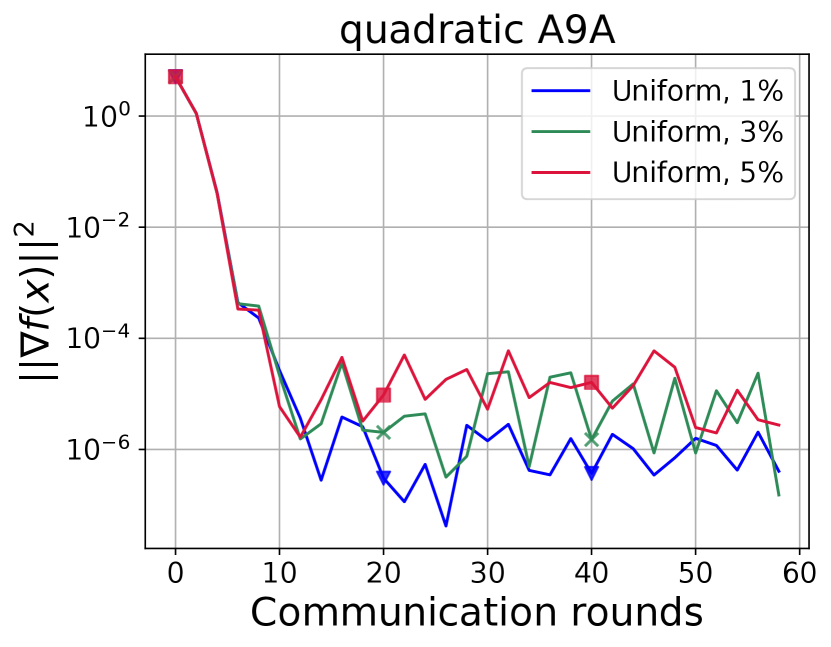
$\bullet$ We investigate how the size of the batches affects the convergence of ASEG on tasks with different parameters. Figure 1 shows the dependence of untuned ASEG convergence on the batch size. In the first experiment the method on $50$ nodes solves the problem with $\mu=0.105$ and $\delta=1.45$. According to Corollary 2 one should choose $B>72\cdot(\nicefrac{{\delta}}{{\mu}})^{\nicefrac{{3}}{{2}}}\approx 3695$ to obtain optimal complexity. That is, for any size of the batch, there is non-optimal rate. In the second experiment, the method on $200$ nodes solves the problem with $\mu=0.06$, $\delta=0.07$. In this case, ASEG has guaranteed optimal complexity for $B>57$ and converges to rather small values of the criterion.

$\bullet$ We compare ASEG to AccSVRS (Figure 2 and Figure 3). 50 nodes are available for Mushrooms and 200 nodes are available for A9A. If the ratio between $\mu$, $\delta$, and $B$ yields the optimal complexity according to Corollary 2, then due to similarity there is an optimistic estimate on the batching noise provides a significant gain over AccSVRS. Otherwise, it is worth using full batching and obtaining a less appreciable gain.

$\bullet$ In ASEG stability experiments (Figure 4, Figure 5, Figure 6, Figure 7) it is tested how white noise in each $\nabla r_{m}(x)$ affects the convergence. It can be seen that increasing the randomness does not worsen the convergence. This can be explained by the fact that the convergence is mainly determined by accuracy of chosen solver.

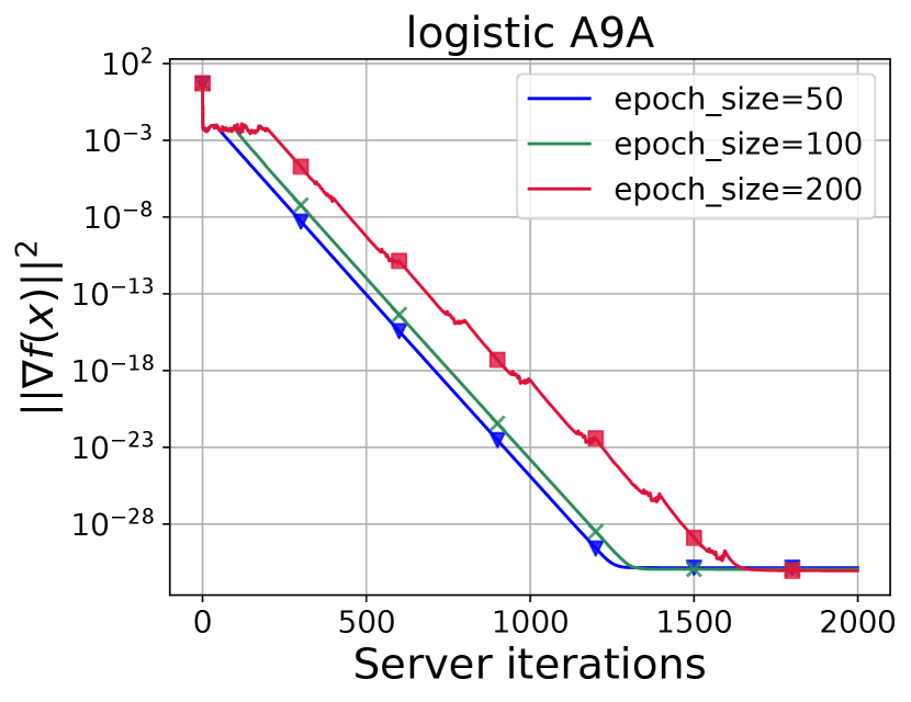
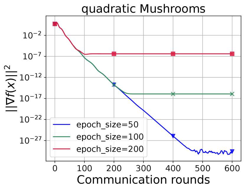
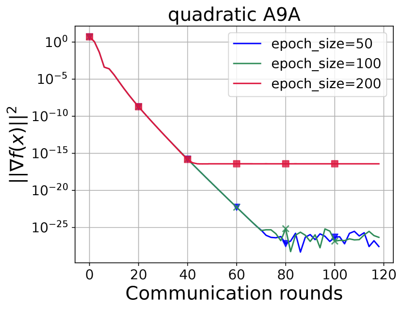
$\bullet$ ASEG experiments test how changing the epoch size changes the ASEG and subproblem (Line 16 of Algorithm 1) convergence with SVRG and SARAH solvers (Figure 8, Figure 9, Figure 10, Figure 11, Figure 12, Figure 13, Figure 14, Figure 15).

Based on the SGD-like approach, we have adapted Accelerated ExtraGradient to solve Federated Learning problems by adding two stochasticities: sampling of computational nodes and application of noise to local gradients. Numerical experiments show that for small values of $\nicefrac{{\delta}}{{\mu}}$ or a sufficiently large number of available nodes, Algorithm 1 (ASEG) is significantly superior to accelerated variance reduction methods (Figure 3), which is consistent with the theory (Corollary 1). If the problem parameters are not "good" enough, there is a $\nicefrac{{\delta^{2}}}{{(\mu^{2}M)}}\cdot\log\nicefrac{{1}}{{\varepsilon}}$ term in the communication complexity of batched ASEG (Corollary 2). Nevertheless, the superiority in the number of communications remains even in this case (Figure 2, Figure 3). Experiments also show the robustness of our method against noise (Figure 4, Figure 5, Figure 6, Figure 7). The server subproblem has also been studied numerically (Figure 10, Figure 11, Figure 14, Figure 15) and theoretically. The analysis shows the inefficiency of randomly choosing the number of solver iterations for the internal subtask (Proposition 2).

References

• Abadi et al., (2016) Abadi, M., Chu, A., Goodfellow, I., McMahan, H. B., Mironov, I., Talwar, K., and Zhang, L. (2016). Deep learning with differential privacy. In Proceedings of the 2016 ACM SIGSAC conference on computer and communications security, pages 308–318.
• Aitsam, (2022) Aitsam, M. (2022). Differential privacy made easy. In 2022 International Conference on Emerging Trends in Electrical, Control, and Telecommunication Engineering (ETECTE), pages 1–7. IEEE.
• Alistarh et al., (2017) Alistarh, D., Grubic, D., Li, J., Tomioka, R., and Vojnovic, M. (2017). Qsgd: Communication-efficient sgd via gradient quantization and encoding. Advances in neural information processing systems, 30.
• Allen-Zhu, (2018) Allen-Zhu, Z. (2018). Katyusha: The first direct acceleration of stochastic gradient methods. Journal of Machine Learning Research, 18(221):1–51.
• Arjevani and Shamir, (2015) Arjevani, Y. and Shamir, O. (2015). Communication complexity of distributed convex learning and optimization. Advances in neural information processing systems, 28.
• Barazandeh et al., (2021) Barazandeh, B., Huang, T., and Michailidis, G. (2021). A decentralized adaptive momentum method for solving a class of min-max optimization problems. Signal Processing, 189:108245.
• Beznosikov et al., (2022) Beznosikov, A., Dvurechenskii, P., Koloskova, A., Samokhin, V., Stich, S. U., and Gasnikov, A. (2022). Decentralized local stochastic extra-gradient for variational inequalities. Advances in Neural Information Processing Systems, 35:38116–38133.
• Beznosikov and Gasnikov, (2022) Beznosikov, A. and Gasnikov, A. (2022). Compression and data similarity: Combination of two techniques for communication-efficient solving of distributed variational inequalities. In International Conference on Optimization and Applications, pages 151–162. Springer.
• Beznosikov et al., (2023) Beznosikov, A., Horváth, S., Richtárik, P., and Safaryan, M. (2023). On biased compression for distributed learning. Journal of Machine Learning Research, 24(276):1–50.
• Beznosikov et al., (2021) Beznosikov, A., Scutari, G., Rogozin, A., and Gasnikov, A. (2021). Distributed saddle-point problems under data similarity. Advances in Neural Information Processing Systems, 34:8172–8184.
• Beznosikov et al., (2024) Beznosikov, A., Takác, M., and Gasnikov, A. (2024). Similarity, compression and local steps: three pillars of efficient communications for distributed variational inequalities. Advances in Neural Information Processing Systems, 36.
• Chang and Lin, (2011) Chang, C.-C. and Lin, C.-J. (2011). Libsvm: A library for support vector machines. ACM transactions on intelligent systems and technology (TIST), 2(3):1–27.
• Defazio et al., (2014) Defazio, A., Bach, F., and Lacoste-Julien, S. (2014). Saga: A fast incremental gradient method with support for non-strongly convex composite objectives. Advances in neural information processing systems, 27.
• Feng et al., (2014) Feng, J., Xu, H., and Mannor, S. (2014). Distributed robust learning. arXiv preprint arXiv:1409.5937.
• Gade and Vaidya, (2018) Gade, S. and Vaidya, N. (2018). Private optimization on networks. pages 1402–1409.
• Gorbunov et al., (2020) Gorbunov, E., Hanzely, F., and Richtárik, P. (2020). A unified theory of sgd: Variance reduction, sampling, quantization and coordinate descent. In International Conference on Artificial Intelligence and Statistics, pages 680–690. PMLR.
• Gorbunov et al., (2021) Gorbunov, E., Hanzely, F., and Richtárik, P. (2021). Local sgd: Unified theory and new efficient methods. In International Conference on Artificial Intelligence and Statistics, pages 3556–3564. PMLR.
• Gorbunov et al., (2019) Gorbunov, E., Hanzely, F., and Richtárik, P. (2019). A unified theory of sgd: Variance reduction, sampling, quantization and coordinate descent.
• Hehn et al., (2020) Hehn, T. M., Kooij, J. F., and Hamprecht, F. A. (2020). End-to-end learning of decision trees and forests. International Journal of Computer Vision, 128(4):997–1011.
• Hendrikx et al., (2020) Hendrikx, H., Xiao, L., Bubeck, S., Bach, F., and Massoulie, L. (2020). Statistically preconditioned accelerated gradient method for distributed optimization. In International conference on machine learning, pages 4203–4227. PMLR.
• Johnson and Zhang, (2013) Johnson, R. and Zhang, T. (2013). Accelerating stochastic gradient descent using predictive variance reduction. Advances in neural information processing systems, 26.
• Khaled and Jin, (2022) Khaled, A. and Jin, C. (2022). Faster federated optimization under second-order similarity. arXiv preprint arXiv:2209.02257.
• Khaled et al., (2020) Khaled, A., Mishchenko, K., and Richtárik, P. (2020). Tighter theory for local sgd on identical and heterogeneous data. In International Conference on Artificial Intelligence and Statistics, pages 4519–4529. PMLR.
• Koloskova et al., (2020) Koloskova, A., Loizou, N., Boreiri, S., Jaggi, M., and Stich, S. (2020). A unified theory of decentralized sgd with changing topology and local updates. In International Conference on Machine Learning, pages 5381–5393. PMLR.
• Kovalev et al., (2022) Kovalev, D., Beznosikov, A., Borodich, E., Gasnikov, A., and Scutari, G. (2022). Optimal gradient sliding and its application to optimal distributed optimization under similarity. Advances in Neural Information Processing Systems, 35:33494–33507.
• Kovalev et al., (2020) Kovalev, D., Horváth, S., and Richtárik, P. (2020). Don’t jump through hoops and remove those loops: Svrg and katyusha are better without the outer loop. In Algorithmic Learning Theory, pages 451–467. PMLR.
• Li et al., (2021) Li, Z., Bao, H., Zhang, X., and Richtárik, P. (2021). Page: A simple and optimal probabilistic gradient estimator for nonconvex optimization. In International conference on machine learning, pages 6286–6295. PMLR.
• Lin et al., (2024) Lin, D., Han, Y., Ye, H., and Zhang, Z. (2024). Stochastic distributed optimization under average second-order similarity: Algorithms and analysis. Advances in Neural Information Processing Systems, 36.
• Lin et al., (2015) Lin, H., Mairal, J., and Harchaoui, Z. (2015). A universal catalyst for first-order optimization. Advances in neural information processing systems, 28.
• McMahan et al., (2017) McMahan, B., Moore, E., Ramage, D., Hampson, S., and y Arcas, B. A. (2017). Communication-efficient learning of deep networks from decentralized data. In Artificial intelligence and statistics, pages 1273–1282. PMLR.
• Moguerza and Muñoz, (2006) Moguerza, J. M. and Muñoz, A. (2006). Support vector machines with applications.
• Nguyen et al., (2017) Nguyen, L. M., Liu, J., Scheinberg, K., and Takáč, M. (2017). Sarah: A novel method for machine learning problems using stochastic recursive gradient. In International conference on machine learning, pages 2613–2621. PMLR.
• Nozari et al., (2016) Nozari, E., Tallapragada, P., and Cortés, J. (2016). Differentially private distributed convex optimization via functional perturbation. IEEE Transactions on Control of Network Systems, 5(1):395–408.
• Sannakki and Kulkarni, (2016) Sannakki, S. and Kulkarni, A. (2016). A review paper on artificial neural network in cognitive science.
• Shalev-Shwartz et al., (2010) Shalev-Shwartz, S., Shamir, O., Srebro, N., and Sridharan, K. (2010). Learnability, stability and uniform convergence. The Journal of Machine Learning Research, 11:2635–2670.
• (36) Shamir, O., Srebro, N., and Zhang, T. (2014a). Communication-efficient distributed optimization using an approximate newton-type method. In International conference on machine learning, pages 1000–1008. PMLR.
• (37) Shamir, O., Srebro, N., and Zhang, T. (2014b). Communication-efficient distributed optimization using an approximate newton-type method. In International conference on machine learning, pages 1000–1008. PMLR.
• Sreenivasan et al., (2006) Sreenivasan, S., Cohen, R., López, E., Toroczkai, Z., and Stanley, H. E. (2006). Communication bottlenecks in scale-free networks. arXiv preprint cs/0604023.
• Stich, (2019) Stich, S. U. (2019). Unified optimal analysis of the (stochastic) gradient method. arXiv preprint arXiv:1907.04232.
• (40) Sun, Y., Scutari, G., and Daneshmand, A. (2022a). Distributed optimization based on gradient tracking revisited: Enhancing convergence rate via surrogation. SIAM Journal on Optimization, 32(2):354–385.
• (41) Sun, Y., Scutari, G., and Daneshmand, A. (2022b). Distributed optimization based on gradient tracking revisited: Enhancing convergence rate via surrogation. SIAM Journal on Optimization, 32(2):354–385.
• Tian et al., (2022) Tian, Y., Scutari, G., Cao, T., and Gasnikov, A. (2022). Acceleration in distributed optimization under similarity. In International Conference on Artificial Intelligence and Statistics, pages 5721–5756. PMLR.
• Tripepi et al., (2008) Tripepi, G., Jager, K., Dekker, F., and Zoccali, C. (2008). Linear and logistic regression analysis. Kidney international, 73(7):806–810.
• Vaswani et al., (2020) Vaswani, S., Laradji, I., Kunstner, F., Meng, S. Y., Schmidt, M., and Lacoste-Julien, S. (2020). Adaptive gradient methods converge faster with over-parameterization (but you should do a line-search). arXiv preprint arXiv:2006.06835.
• Verbraeken et al., (2020) Verbraeken, J., Wolting, M., Katzy, J., Kloppenburg, J., Verbelen, T., and Rellermeyer, J. S. (2020). A survey on distributed machine learning. Acm computing surveys (csur), 53(2):1–33.
• Weeraddana and Fischione, (2017) Weeraddana, P. and Fischione, C. (2017). On the privacy of optimization. IFAC-PapersOnLine, 50(1):9502–9508.
• Woodworth et al., (2020) Woodworth, B. E., Patel, K. K., and Srebro, N. (2020). Minibatch vs local sgd for heterogeneous distributed learning. Advances in Neural Information Processing Systems, 33:6281–6292.
• Yuan and Li, (2020) Yuan, X.-T. and Li, P. (2020). On convergence of distributed approximate newton methods: Globalization, sharper bounds and beyond. Journal of Machine Learning Research, 21(206):1–51.
In all the appendices, we consider r1(x)=q(x)r_{1}(x)=q(x) and p(x)=r(x)r1(x)p(x)=r(x)-r_{1}(x). Mathematical expectations are implied in the context of the proof.
Appendix A Lemma 1
Here we prove Lemma 1. First, we need the following:
Lemma 2.
Consider Algorithm 1. Let θ\theta be defined as in Lemma 1: θ13δ\theta\leq\frac{1}{3\delta}. Then under Assumptions 1 and 3, the following inequality holds for all x¯d\bar{x}\in\mathbb{R}^{d}:
𝔼[2x¯xgk,tk|xk,xfk+1]2[r(x¯)r(xfk+1)]μxfk+1x¯2θr(xfk+1)2+11θ3(A¯θk(xfk+1)29δ211xgkargminxdA¯θk(x)2)+3θp(xgk)sk2.\begin{split}\mathbb{E}\big{[}2\langle\bar{x}-x_{g}^{k},t_{k}\rangle\big{|}&x^{k},x_{f}^{k+1}\big{]}\\ \leq&2\left[r(\bar{x})-r(x_{f}^{k+1})\right]-\mu\lVert x_{f}^{k+1}-\bar{x}\rVert^{2}-\theta\lVert\nabla r(x_{f}^{k+1})\rVert^{2}\\ &+\frac{11\theta}{3}\left(\lVert\nabla\bar{A}_{\theta}^{k}(x_{f}^{k+1})\rVert^{2}-\frac{9\delta^{2}}{11}\lVert x_{g}^{k}-\arg\min_{x\in\mathbb{R}^{d}}\bar{A}_{\theta}^{k}(x)\rVert^{2}\right)\\ &+3\theta\lVert\nabla p(x_{g}^{k})-s_{k}\rVert^{2}.\end{split} (11)
Proof.
Using the μ\mu-strong convexity of r(x)r(x), we get
𝔼[2x¯xgk,tk|xk,xfk+1]=\displaystyle\mathbb{E}\big{[}2\langle\bar{x}-x_{g}^{k},t_{k}\rangle\big{|}x^{k},x_{f}^{k+1}\big{]}= 2x¯xgk,𝔼[tk|xk,xfk+1]\displaystyle 2\langle\bar{x}-x_{g}^{k},\mathbb{E}\big{[}t_{k}\big{|}x^{k},x_{f}^{k+1}\big{]}\rangle
=\displaystyle= 2x¯xgk,r(xfk+1)\displaystyle 2\langle\bar{x}-x_{g}^{k},\nabla r(x_{f}^{k+1})\rangle
=\displaystyle= 2x¯xfk+1,r(xfk+1)+2xfk+1xgk,r(xfk+1)\displaystyle 2\langle\bar{x}-x_{f}^{k+1},\nabla r(x_{f}^{k+1})\rangle+2\langle x_{f}^{k+1}-x_{g}^{k},\nabla r(x_{f}^{k+1})\rangle
\displaystyle\leq 2[r(x¯)r(xfk+1)]μxfk+1x¯2\displaystyle 2\left[r(\bar{x})-r(x_{f}^{k+1})\right]-\mu\lVert x_{f}^{k+1}-\bar{x}\rVert^{2}
+2xfk+1xgk,r(xfk+1)\displaystyle+2\langle x_{f}^{k+1}-x_{g}^{k},\nabla r(x_{f}^{k+1})\rangle
=\displaystyle= 2[r(x¯)r(xfk+1)]μxfk+1x¯2\displaystyle 2\left[r(\bar{x})-r(x_{f}^{k+1})\right]-\mu\lVert x_{f}^{k+1}-\bar{x}\rVert^{2}
+2θθ1(xfk+1xgk),r(xfk+1).\displaystyle+2\theta\left\langle\theta^{-1}(x_{f}^{k+1}-x_{g}^{k}),\nabla r(x_{f}^{k+1})\right\rangle.
From the properties of the norm we can write
xfk+1xgkθ+r(xfk+1)2=\displaystyle\left\|\frac{x_{f}^{k+1}-x_{g}^{k}}{\theta}+\nabla r(x_{f}^{k+1})\right\|^{2}= 1θ2xfk+1xgk2+r(xfk+1)2\displaystyle\frac{1}{\theta^{2}}\|x_{f}^{k+1}-x_{g}^{k}\|^{2}+\|\nabla r(x_{f}^{k+1})\|^{2}
+2θxfk+1xgk,r(xfk+1).\displaystyle+\frac{2}{\theta}\left\langle x_{f}^{k+1}-x_{g}^{k},\nabla r(x_{f}^{k+1})\right\rangle.
Thus,
𝔼[2x¯xgk,tk|xk,xfk+1]=\displaystyle\mathbb{E}\big{[}2\langle\bar{x}-x_{g}^{k},t_{k}\rangle\big{|}x^{k},x_{f}^{k+1}\big{]}= 2[r(x¯)r(xfk+1)]μxfk+1x¯21θxfk+1xgk2\displaystyle 2\left[r(\bar{x})-r(x_{f}^{k+1})\right]-\mu\lVert x_{f}^{k+1}-\bar{x}\rVert^{2}-\frac{1}{\theta}\lVert x_{f}^{k+1}-x_{g}^{k}\rVert^{2}
θr(xfk+1)2+θθ1(xfk+1xgk)+r(xfk+1)2.\displaystyle-\theta\lVert\nabla r(x_{f}^{k+1})\rVert^{2}+\theta\lVert\theta^{-1}(x_{f}^{k+1}-x_{g}^{k})+\nabla r(x_{f}^{k+1})\rVert^{2}.
The definition of A¯θk(x)\bar{A}_{\theta}^{k}(x) and δ\delta-Lipschitzness of p\nabla p give
𝔼[2x¯xgk,tk|\displaystyle\mathbb{E}\big{[}2\langle\bar{x}-x_{g}^{k},t_{k}\rangle\big{|} xk,xfk+1]\displaystyle x^{k},x_{f}^{k+1}\big{]}
\displaystyle\leq 2[r(x¯)r(xfk+1)]μxfk+1x¯21θxfk+1xgk2\displaystyle 2\left[r(\bar{x})-r(x_{f}^{k+1})\right]-\mu\lVert x_{f}^{k+1}-\bar{x}\rVert^{2}-\frac{1}{\theta}\lVert x_{f}^{k+1}-x_{g}^{k}\rVert^{2}
+θA¯θk(xfk+1)+p(xfk+1)p(xgk)+p(xgk)sk)2\displaystyle+\theta\lVert\nabla\bar{A}_{\theta}^{k}(x_{f}^{k+1})+\nabla p(x_{f}^{k+1})-\nabla p(x_{g}^{k})+\nabla p(x_{g}^{k})-s_{k})\rVert^{2}
θr(xfk+1)2\displaystyle-\theta\lVert\nabla r(x_{f}^{k+1})\rVert^{2}
Note that
a+b+c23a2+3b2+3c2,\displaystyle\|a+b+c\|^{2}\leq 3\|a\|^{2}+3\|b\|^{2}+3\|c\|^{2},
and the Hessian similarity (Definition 3) implies
p(xfk+1)p(xgk)2δ2xfk+1xgk2.\displaystyle\|\nabla p(x_{f}^{k+1})-\nabla p(x_{g}^{k})\|^{2}\leq\delta^{2}\|x_{f}^{k+1}-x_{g}^{k}\|^{2}.
𝔼[2x¯xgk,tk|xk,xfk+1]\displaystyle\mathbb{E}\big{[}2\langle\bar{x}-x_{g}^{k},t_{k}\rangle\big{|}x^{k},x_{f}^{k+1}\big{]}\leq 2[r(x¯)r(xfk+1)]μxfk+1x¯21θxfk+1xgk2\displaystyle 2\left[r(\bar{x})-r(x_{f}^{k+1})\right]-\mu\lVert x_{f}^{k+1}-\bar{x}\rVert^{2}-\frac{1}{\theta}\lVert x_{f}^{k+1}-x_{g}^{k}\rVert^{2}
θr(xfk+1)2+3θA¯θk(xfk+1)2\displaystyle-\theta\lVert\nabla r(x_{f}^{k+1})\rVert^{2}+3\theta\lVert\nabla\bar{A}_{\theta}^{k}(x_{f}^{k+1})\rVert^{2}
+3θδ2xfk+1xgk2+3θp(xgk)sk2\displaystyle+3\theta\delta^{2}\lVert x_{f}^{k+1}-x_{g}^{k}\rVert^{2}+3\theta\lVert\nabla p(x_{g}^{k})-s_{k}\rVert^{2}
1θ(13θ2δ2)xfk+1xgk2θr(xfk+1)2\displaystyle-\frac{1}{\theta}\left(1-3\theta^{2}\delta^{2}\right)\lVert x_{f}^{k+1}-x_{g}^{k}\rVert^{2}-\theta\lVert\nabla r(x_{f}^{k+1})\rVert^{2}
+3θA¯θk(xfk+1)2+3θp(xgk)sk2.\displaystyle+3\theta\lVert\nabla\bar{A}_{\theta}^{k}(x_{f}^{k+1})\rVert^{2}+3\theta\lVert\nabla p(x_{g}^{k})-s_{k}\rVert^{2}.
With θ13δ\theta\leq\frac{1}{3\delta}, we have
𝔼[2x¯xgk,tk|xk,xfk+1]\displaystyle\mathbb{E}\big{[}2\langle\bar{x}-x_{g}^{k},t_{k}\rangle\big{|}x^{k},x_{f}^{k+1}\big{]}\leq 2[r(x¯)r(xfk+1)]μxfk+1x¯223θxfk+1xgk2\displaystyle 2\left[r(\bar{x})-r(x_{f}^{k+1})\right]-\mu\lVert x_{f}^{k+1}-\bar{x}\rVert^{2}-\frac{2}{3\theta}\lVert x_{f}^{k+1}-x_{g}^{k}\rVert^{2}
+3θp(xgk)sk2\displaystyle+3\theta\lVert\nabla p(x_{g}^{k})-s_{k}\rVert^{2}
\displaystyle\leq 2[r(x¯)r(xfk+1)]μxfk+1x¯2θr(xfk+1)2\displaystyle 2\left[r(\bar{x})-r(x_{f}^{k+1})\right]-\mu\lVert x_{f}^{k+1}-\bar{x}\rVert^{2}-\theta\lVert\nabla r(x_{f}^{k+1})\rVert^{2}
+3θA¯θk(xfk+1)2+3θp(xgk)sk2\displaystyle+3\theta\lVert\nabla\bar{A}_{\theta}^{k}(x_{f}^{k+1})\rVert^{2}+3\theta\lVert\nabla p(x_{g}^{k})-s_{k}\rVert^{2}
13θxgkargminxdA¯θk(x)2\displaystyle-\frac{1}{3\theta}\lVert x_{g}^{k}-\arg\min_{x\in\mathbb{R}^{d}}\bar{A}_{\theta}^{k}(x)\rVert^{2}
+23θxfk+1argminxdA¯θk(x)2.\displaystyle+\frac{2}{3\theta}\lVert x_{f}^{k+1}-\arg\min_{x\in\mathbb{R}^{d}}\bar{A}_{\theta}^{k}(x)\rVert^{2}.
Here we used the fact that:
ac212ab2+bc2.\displaystyle-\|a-c\|^{2}\leq-\frac{1}{2}\|a-b\|^{2}+\|b-c\|^{2}.
One can observe that Aθk(x)A_{\theta}^{k}(x) is 1θ\frac{1}{\theta}-strongly convex. Hence,
𝔼[2x¯xgk,tk|xk,xfk+1]\displaystyle\mathbb{E}\big{[}2\langle\bar{x}-x_{g}^{k},t_{k}\rangle\big{|}x^{k},x_{f}^{k+1}\big{]}\leq 2[r(x¯)r(xfk+1)]μxfk+1x¯2θr(xfk+1)2\displaystyle 2\left[r(\bar{x})-r(x_{f}^{k+1})\right]-\mu\lVert x_{f}^{k+1}-\bar{x}\rVert^{2}-\theta\lVert\nabla r(x_{f}^{k+1})\rVert^{2}
13θxgkargminxdA¯θk(x)2+2θ3A¯θk(xfk+1)2.\displaystyle-\frac{1}{3\theta}\lVert x_{g}^{k}-\arg\min_{x\in\mathbb{R}^{d}}\bar{A}_{\theta}^{k}(x)\rVert^{2}+\frac{2\theta}{3}\lVert\nabla\bar{A}_{\theta}^{k}(x_{f}^{k+1})\rVert^{2}.
Now we are ready to construct the expression with the convergence criterion.
+11θ3(A¯θk(xfk+1)2111θ2xgkargminxdA¯θk(x)2)\displaystyle+\frac{11\theta}{3}\left(\lVert\nabla\bar{A}_{\theta}^{k}(x_{f}^{k+1})\rVert^{2}-\frac{1}{11\theta^{2}}\lVert x_{g}^{k}-\arg\min_{x\in\mathbb{R}^{d}}\bar{A}_{\theta}^{k}(x)\rVert^{2}\right)
=\displaystyle=  2[r(x¯)r(xfk+1)]μxfk+1x¯2θr(xfk+1)2\displaystyle\;2\left[r(\bar{x})-r(x_{f}^{k+1})\right]-\mu\lVert x_{f}^{k+1}-\bar{x}\rVert^{2}-\theta\lVert\nabla r(x_{f}^{k+1})\rVert^{2}
+11θ3(A¯θk(xfk+1)29δ211xgkargminxdA¯θk(x)2)\displaystyle+\frac{11\theta}{3}\left(\lVert\nabla\bar{A}_{\theta}^{k}(x_{f}^{k+1})\rVert^{2}-\frac{9\delta^{2}}{11}\lVert x_{g}^{k}-\arg\min_{x\in\mathbb{R}^{d}}\bar{A}_{\theta}^{k}(x)\rVert^{2}\right)
+3θp(xgk)sk2.\displaystyle+3\theta\lVert\nabla p(x_{g}^{k})-s_{k}\rVert^{2}.
This completes the proof of Lemma 2. ∎
Let us move on to proof of Lemma 1:
Lemma 3.
(Lemma 1) Under Assumptions 1, 2 and 3, the condition (4) and the tuning (3) we obtain:
𝔼[1η\displaystyle\mathbb{E}\bigg{[}\frac{1}{\eta} xk+1x2+2τ[r(xfk+1)r(x)]]\displaystyle\lVert x^{k+1}-x^{*}\rVert^{2}+\frac{2}{\tau}\left[r(x_{f}^{k+1})-r(x^{*})\right]\bigg{]}
\displaystyle\leq (1αη+12θδ2ηBζ)𝔼[1ηxkx2]+(1τ)𝔼[2τ[r(xfk)r(x)]]\displaystyle\left(1-\alpha\eta+\frac{12\theta\delta^{2}\eta}{B}\cdot\zeta\right)\cdot\mathbb{E}\left[\frac{1}{\eta}\lVert x^{k}-x^{*}\rVert^{2}\right]+(1-\tau)\cdot\mathbb{E}\left[\frac{2}{\tau}\left[r(x_{f}^{k})-r(x^{*})\right]\right]
+𝔼[(12θδ2Bτμ6)ζ(xfkx2+xfk+1x2)]+4θBτσ2.\displaystyle+\mathbb{E}\left[\left(\frac{12\theta\delta^{2}}{B\tau}-\frac{\mu}{6}\right)\cdot\zeta\left(\|x_{f}^{k}-x_{*}\|^{2}+\|x_{f}^{k+1}-x_{*}\|^{2}\right)\right]+\frac{4\theta}{B\tau}\sigma^{2}.
Using Line 27, we write
1ηxk+1x2=\displaystyle\frac{1}{\eta}\lVert x^{k+1}-x^{*}\rVert^{2}= 1ηxkx2+2ηxk+1xk,xkx+1ηxk+1xk2\displaystyle\frac{1}{\eta}\lVert x^{k}-x^{*}\rVert^{2}+\frac{2}{\eta}\langle x^{k+1}-x^{k},x^{k}-x^{*}\rangle+\frac{1}{\eta}\lVert x^{k+1}-x^{k}\rVert^{2}
=\displaystyle= 1ηxkx2+2αxfk+1xk,xkx2tk,xkx\displaystyle\frac{1}{\eta}\lVert x^{k}-x^{*}\rVert^{2}+2\alpha\langle x_{f}^{k+1}-x^{k},x^{k}-x^{*}\rangle-2\langle t_{k},x^{k}-x^{*}\rangle
+1ηxk+1xk2\displaystyle+\frac{1}{\eta}\lVert x^{k+1}-x^{k}\rVert^{2}
=\displaystyle= 1ηxkx2+αxfk+1x2αxkx2\displaystyle\frac{1}{\eta}\lVert x^{k}-x^{*}\rVert^{2}+\alpha\lVert x_{f}^{k+1}-x^{*}\rVert^{2}-\alpha\lVert x^{k}-x^{*}\rVert^{2}
αxfk+1xk22tk,xkx+1ηxk+1xk2,\displaystyle-\alpha\lVert x_{f}^{k+1}-x^{k}\rVert^{2}-2\langle t_{k},x^{k}-x^{*}\rangle+\frac{1}{\eta}\lVert x^{k+1}-x^{k}\rVert^{2},
Here we use the properties of the norm to reveal the inner product. Line 5 of Algorithm 1 gives
1ηxk+1x2=\displaystyle\frac{1}{\eta}\lVert x^{k+1}-x^{*}\rVert^{2}= (1ηα)xkx2+αxfk+1x2+1ηxk+1xk2\displaystyle\left(\frac{1}{\eta}-\alpha\right)\lVert x^{k}-x^{*}\rVert^{2}+\alpha\lVert x_{f}^{k+1}-x^{*}\rVert^{2}+\frac{1}{\eta}\lVert x^{k+1}-x^{k}\rVert^{2}
αxfk+1xk2+2tk,xxgk+2(1τ)τtk,xfkxgk.\displaystyle-\alpha\lVert x_{f}^{k+1}-x^{k}\rVert^{2}+2\langle t_{k},x^{*}-x_{g}^{k}\rangle+\frac{2(1-\tau)}{\tau}\langle t_{k},x_{f}^{k}-x_{g}^{k}\rangle.
Using (11) with x¯=x\bar{x}=x^{*} and x¯=xfk\bar{x}=x_{f}^{k}, we get
𝔼[1ηxk+1x2|xk,xfk+1]\displaystyle\mathbb{E}\left[\frac{1}{\eta}\lVert x^{k+1}-x^{*}\rVert^{2}\Bigg{|}x^{k},x_{f}^{k+1}\right]\leq (1ηα)xkx2+αxfk+1x2\displaystyle\left(\frac{1}{\eta}-\alpha\right)\lVert x^{k}-x^{*}\rVert^{2}+\alpha\lVert x_{f}^{k+1}-x^{*}\rVert^{2}
+𝔼[1ηxk+1xk2|xk,xfk+1]αxfk+1xk2\displaystyle+\mathbb{E}\left[\frac{1}{\eta}\lVert x^{k+1}-x^{k}\rVert^{2}\Bigg{|}x^{k},x_{f}^{k+1}\right]-\alpha\lVert x_{f}^{k+1}-x^{k}\rVert^{2}
+2[r(x)r(xfk+1)]μxfk+1x2\displaystyle+2\left[r(x^{*})-r(x_{f}^{k+1})\right]-\mu\lVert x_{f}^{k+1}-x^{*}\rVert^{2}
+2(1τ)τ[r(xfk)r(xfk+1)]θτr(xfk+1)2\displaystyle+\frac{2(1-\tau)}{\tau}\left[r(x_{f}^{k})-r(x_{f}^{k+1})\right]-\frac{\theta}{\tau}\lVert\nabla r(x_{f}^{k+1})\rVert^{2}
μxfk+1xfk2+3θτp(xgk)sk2\displaystyle-\mu\|x_{f}^{k+1}-x_{f}^{k}\|^{2}+\frac{3\theta}{\tau}\lVert\nabla p(x_{g}^{k})-s_{k}\rVert^{2}
+11θ3τ(A¯θk(xfk+1)29δ211xgkargminxdA¯θk(x)2).\displaystyle+\frac{11\theta}{3\tau}\left(\lVert\nabla\bar{A}_{\theta}^{k}(x_{f}^{k+1})\rVert^{2}-\frac{9\delta^{2}}{11}\lVert x_{g}^{k}-\arg\min_{x\in\mathbb{R}^{d}}\bar{A}_{\theta}^{k}(x)\rVert^{2}\right).
The last expression
11θ3τ(A¯θk(xfk+1)29δ211xgkargminxdA¯θk(x)2),\displaystyle\frac{11\theta}{3\tau}\left(\lVert\nabla\bar{A}_{\theta}^{k}(x_{f}^{k+1})\rVert^{2}-\frac{9\delta^{2}}{11}\lVert x_{g}^{k}-\arg\min_{x\in\mathbb{R}^{d}}\bar{A}_{\theta}^{k}(x)\rVert^{2}\right),
can be neglected due to the condition (4). Consider expectation separately:
𝔼[1ηxk+1xk2|xk,xfk+1]=\displaystyle\mathbb{E}\left[\frac{1}{\eta}\lVert x^{k+1}-x^{k}\rVert^{2}\Bigg{|}x^{k},x_{f}^{k+1}\right]= 1η𝔼[ηα(xfk+1xk)ηtk2|xk,xfk+1]\displaystyle\frac{1}{\eta}\mathbb{E}\left[\lVert\eta\alpha(x_{f}^{k+1}-x^{k})-\eta t_{k}\rVert^{2}\Big{|}x^{k},x_{f}^{k+1}\right]
\displaystyle\leq 3ηα2xfk+1xk2+3ηr(xfk+1)2\displaystyle 3\eta\alpha^{2}\lVert x_{f}^{k+1}-x^{k}\rVert^{2}+3\eta\lVert\nabla r(x_{f}^{k+1})\rVert^{2}
+3η𝔼[r(xfk+1)tk2|xk,xfk+1].\displaystyle+3\eta\mathbb{E}\left[\lVert\nabla r(x_{f}^{k+1})-t_{k}\rVert^{2}\Big{|}x^{k},x_{f}^{k+1}\right].
Here we added and subtracted ηr(xfk+1)\eta\nabla r(x_{f}^{k+1}) under the norm. After rearranging the expressions, we obtain
𝔼[1ηxk+1x2|xk,xfk+1]\displaystyle\mathbb{E}\left[\frac{1}{\eta}\lVert x^{k+1}-x^{*}\rVert^{2}\Bigg{|}x^{k},x_{f}^{k+1}\right]\leq (1ηα)xkx2+(αμ3)xfk+1x2\displaystyle\left(\frac{1}{\eta}-\alpha\right)\lVert x^{k}-x^{*}\rVert^{2}+(\alpha-\frac{\mu}{3})\lVert x_{f}^{k+1}-x^{*}\rVert^{2}
+α(3ηα1)xfk+1xk2+3θτp(xgk)sk2\displaystyle+\alpha(3\eta\alpha-1)\lVert x_{f}^{k+1}-x^{k}\rVert^{2}+\frac{3\theta}{\tau}\lVert\nabla p(x_{g}^{k})-s_{k}\rVert^{2}
+2(1τ)τ[r(xfk)r(x)]2τ[r(xfk+1)r(x)]\displaystyle+\frac{2(1-\tau)}{\tau}\left[r(x_{f}^{k})-r(x^{*})\right]-\frac{2}{\tau}\left[r(x_{f}^{k+1})-r(x^{*})\right]
+3ηr(xfk+1)tk2μ3xfk+1x2\displaystyle+3\eta\lVert\nabla r(x_{f}^{k+1})-t_{k}\rVert^{2}-\frac{\mu}{3}\|x_{f}^{k+1}-x_{*}\|^{2}
μ3xfk+1x2μxfk+1xfk2\displaystyle-\frac{\mu}{3}\|x_{f}^{k+1}-x_{*}\|^{2}-\mu\|x_{f}^{k+1}-x_{f}^{k}\|^{2}
+(3ηθτ)r(xfk+1)2.\displaystyle+\left(3\eta-\frac{\theta}{\tau}\right)\lVert\nabla r(x_{f}^{k+1})\rVert^{2}.
The choice of α,η,τ\alpha,\eta,\tau defined by (3) gives
𝔼[1ηxk+1x2|xk,xfk+1]\displaystyle\mathbb{E}\left[\frac{1}{\eta}\lVert x^{k+1}-x^{*}\rVert^{2}\Bigg{|}x^{k},x_{f}^{k+1}\right]\leq (1ηα)xkx2+2(1τ)τ[r(xfk)r(x)]\displaystyle\left(\frac{1}{\eta}-\alpha\right)\lVert x^{k}-x^{*}\rVert^{2}+\frac{2(1-\tau)}{\tau}\left[r(x_{f}^{k})-r(x^{*})\right]
2τ[r(xfk+1)r(x)]+3θτp(xgk)sk2\displaystyle-\frac{2}{\tau}\left[r(x_{f}^{k+1})-r(x^{*})\right]+\frac{3\theta}{\tau}\lVert\nabla p(x_{g}^{k})-s_{k}\rVert^{2}
+θτr(xfk+1)tk2μ3xfk+1x2\displaystyle+\frac{\theta}{\tau}\lVert\nabla r(x_{f}^{k+1})-t_{k}\rVert^{2}-\frac{\mu}{3}\|x_{f}^{k+1}-x_{*}\|^{2}
μ3xfk+1x2μxfk+1xfk2.\displaystyle-\frac{\mu}{3}\|x_{f}^{k+1}-x_{*}\|^{2}-\mu\|x_{f}^{k+1}-x_{f}^{k}\|^{2}.
μ3xfk+1x2μ6xfkx2+μ3xfk+1xfk2.\displaystyle-\frac{\mu}{3}\|x_{f}^{k+1}-x_{*}\|^{2}\leq-\frac{\mu}{6}\|x_{f}^{k}-x_{*}\|^{2}+\frac{\mu}{3}\|x_{f}^{k+1}-x_{f}^{k}\|^{2}.
Here we need a technical lemma:
Lemma 4.
Let p(x)=r(x)r1(x)p(x)=r(x)-r_{1}(x) and sk=1Bi=1B(rmi(xgk,ξ)r1(xgk))s_{k}=\frac{1}{B}\sum_{i=1}^{B}(\nabla r_{m_{i}}(x_{g}^{k},\xi)-\nabla r_{1}(x_{g}^{k})). Then:
𝔼ξ,i[skp(xgk)2]2(σsim2+σnoise2)B+4δ2Bxfk+1x2ζ.\displaystyle\mathbb{E}_{\xi,i}\left[\|s_{k}-\nabla p(x_{g}^{k})\|^{2}\right]\leq\frac{2(\sigma_{sim}^{2}+\sigma_{noise}^{2})}{B}+\frac{4\delta^{2}}{B}\|x_{f}^{k+1}-x_{*}\|^{2}\cdot\zeta.
Let us apply the Young’s inequality
𝔼ξ,i[skp(xgk)2]\displaystyle\mathbb{E}_{\xi,i}[\|s_{k}-\nabla p(x_{g}^{k})\|^{2}]
=\displaystyle= 𝔼ξ,i[r(xgk)1Bi=1Brmi(xgk,ξi)±1Bi=1Brmi(xgk)2]\displaystyle\mathbb{E}_{\xi,i}\left[\left\|\nabla r(x_{g}^{k})-\frac{1}{B}\sum_{i=1}^{B}\nabla r_{m_{i}}(x_{g}^{k},\xi_{i})\pm\frac{1}{B}\sum_{i=1}^{B}\nabla r_{m_{i}}(x_{g}^{k})\right\|^{2}\right]
\displaystyle\leq 2𝔼i[r(xgk)1Bi=1Brmi(xgk)2]\displaystyle 2\mathbb{E}_{i}\left[\left\|\nabla r(x_{g}^{k})-\frac{1}{B}\sum_{i=1}^{B}\nabla r_{m_{i}}(x_{g}^{k})\right\|^{2}\right]
+2B2𝔼i,ξi=1B(rmi(xgk)rmi(xgk,ξi))2.\displaystyle+\frac{2}{B^{2}}\mathbb{E}_{i,\xi}\left\|\sum_{i=1}^{B}(\nabla r_{m_{i}}(x_{g}^{k})-\nabla r_{m_{i}}(x_{g}^{k},\xi_{i}))\right\|^{2}.
Next, we look at the expression, given by the second term:
2B2i=1Brmi(xgk)rmi(xgk,ξi)2\displaystyle\frac{2}{B^{2}}\sum_{i=1}^{B}\|\nabla r_{m_{i}}(x_{g}^{k})-\nabla r_{m_{i}}(x_{g}^{k},\xi_{i})\|^{2}
+2B2ij=1Brmi(xgk)rmi(xgk,ξi),rmj(xgk)rmj(xgk,ξj).\displaystyle+\frac{2}{B^{2}}\sum_{i\neq j=1}^{B}\langle\nabla r_{m_{i}}(x_{g}^{k})-\nabla r_{m_{i}}(x_{g}^{k},\xi_{i}),\nabla r_{m_{j}}(x_{g}^{k})-\nabla r_{m_{j}}(x_{g}^{k},\xi_{j})\rangle.
Let us use the tower property and take the ξ\xi expectation first. Since mim_{i} and mjm_{j} are independent, we can enter the expectation into the multipliers of the second summand separately. Then only the first summand will remain, which is estimated based on Assumption 2. Using Assumption 2, we obtain
Let us return to the proof of the lemma. Denote σ2=2(σsim2+σnoise2)\sigma^{2}=2(\sigma_{sim}^{2}+\sigma_{noise}^{2}). Taking expectation and with (4), we have
\displaystyle\leq 𝔼[(1ηα+12θδ2Bζ)xkx2]\displaystyle\mathbb{E}\left[\left(\frac{1}{\eta}-\alpha+\frac{12\theta\delta^{2}}{B}\cdot\zeta\right)\lVert x^{k}-x^{*}\rVert^{2}\right]
+𝔼[2(1τ)τ[r(xfk)r(x)]]\displaystyle+\mathbb{E}\left[\frac{2(1-\tau)}{\tau}\left[r(x_{f}^{k})-r(x^{*})\right]\right]
+𝔼[(12θδ2Bτμ6)xfkx2ζ]\displaystyle+\mathbb{E}\left[\left(\frac{12\theta\delta^{2}}{B\tau}-\frac{\mu}{6}\right)\|x_{f}^{k}-x_{*}\|^{2}\cdot\zeta\right]
+𝔼[(4θδ2Bτμ3)xfk+1x2ζ]\displaystyle+\mathbb{E}\left[\left(\frac{4\theta\delta^{2}}{B\tau}-\frac{\mu}{3}\right)\|x_{f}^{k+1}-x_{*}\|^{2}\cdot\zeta\right]
+4θBτσ2.\displaystyle+\frac{4\theta}{B\tau}\sigma^{2}.
Appendix B Theorem 2
Theorem 5.
(Theorem 2) In Lemma 1 choose ζ=1\zeta=1 and the tuning (6). Then we have:
𝔼[Φk+1](1μθ18)𝔼[Φk]+4θB,\displaystyle\mathbb{E}[\Phi_{k+1}]\leq\left(1-\frac{\sqrt{\mu\theta}}{18}\right)\mathbb{E}[\Phi_{k}]+\frac{4\theta}{B},
where Φk=τηxkx2+2[r(xfk)r(x)]\Phi_{k}=\frac{\tau}{\eta}\|x^{k}-x^{*}\|^{2}+2[r(x_{f}^{k})-r(x^{*})].
We consider possible values of η\eta one by one.
\bullet Consider η=1μ\eta=\frac{1}{\mu}. In this case, we have:
1\displaystyle 1 ηα+12ηθδ2B23+12δ2BμμBτ72δ256=116.\displaystyle-\eta\alpha+\frac{12\eta\theta\delta^{2}}{B}\leq\frac{2}{3}+\frac{12\delta^{2}}{B\mu}\frac{\mu B\tau}{72\delta^{2}}\leq\frac{5}{6}=1-\frac{1}{6}.
\bullet Consider ηθ3τ\eta-\frac{\theta}{3\tau}:
1ηα+12ηθδ2B=\displaystyle 1-\eta\alpha+\frac{12\eta\theta\delta^{2}}{B}= 1μθ9τ+4θ2δ2Bτ1μθ9τ+4θδ2BτμBτ72δ21μθ18τ\displaystyle 1-\frac{\mu\theta}{9\tau}+\frac{4\theta^{2}\delta^{2}}{B\tau}\leq 1-\frac{\mu\theta}{9\tau}+\frac{4\theta\delta^{2}}{B\tau}\frac{\mu B\tau}{72\delta^{2}}\leq 1-\frac{\mu\theta}{18\tau}
=\displaystyle= 1μθ18.\displaystyle 1-\frac{\sqrt{\mu\theta}}{18}.
Thus, we obtain:
𝔼[Φk+1]max{116,1μθ18}.\displaystyle\mathbb{E}[\Phi_{k+1}]\leq\max\left\{1-\frac{1}{6},1-\frac{\sqrt{\mu\theta}}{18}\right\}.
Since μ<δ\mu<\delta, we obtain the required. ∎
Appendix C Corrolary 1, 2
Here we introduce a proof for Corollary 1 and Corollary 2. We use tecnhique from (Stich,, 2019).
Earlier we obtained the recurrence formula:
0(1aθ)𝔼[Φk]𝔼[Φk+1]+cθ.\displaystyle 0\leq(1-a\sqrt{\theta})\mathbb{E}[\Phi_{k}]-\mathbb{E}[\Phi_{k+1}]+c\theta.
Let us multiply both sides by weight wk=(1aθ)(k+1)w_{k}=(1-a\sqrt{\theta})^{-(k+1)} and rewrite:
01θ(𝔼[Φk]wk1𝔼[Φk+1]wk)+cwkθ.\displaystyle 0\leq\frac{1}{\sqrt{\theta}}\left(\mathbb{E}[\Phi_{k}]w_{k-1}-\mathbb{E}[\Phi_{k+1}]w_{k}\right)+cw_{k}\sqrt{\theta}.
Denote WN=k=0Nwk(1θ)(N+1)k=0N(1aθ)kwNaθW_{N}=\sum_{k=0}^{N}w_{k}(1-\sqrt{\theta})^{-(N+1)}\sum_{k=0}^{N}(1-a\sqrt{\theta})^{k}\leq\frac{w_{N}}{a\sqrt{\theta}} and sum up with k=0,,Nk=0,...,N:
wN𝔼[Φk+1]θWNΦ0θWN+cθ.\displaystyle\frac{w_{N}\mathbb{E}[\Phi_{k+1}]}{\sqrt{\theta}W_{N}}\leq\frac{\Phi_{0}}{\sqrt{\theta}W_{N}}+c\sqrt{\theta}.
Let us rewrite:
𝔼[Φk+1]1aθexp{aθ(N+1)}+cθa.\displaystyle\mathbb{E}[\Phi_{k+1}]\leq\frac{1}{a\sqrt{\theta}}\exp\{-a\sqrt{\theta}(N+1)\}+\frac{c\sqrt{\theta}}{a}.
To complete the proof we need to substitute a=μ3a=\frac{\sqrt{\mu}}{3} and c=4σ2Bc=\frac{4\sigma^{2}}{B} for Corollary 1 and a=μ18a=\frac{\sqrt{\mu}}{18} and c=4σ2Bc=\frac{4\sigma^{2}}{B} for Corollary 2 and look at different θ\theta.
For Corollary 1 we obtain:
If 9ln2(max{2,BμN2Φ036σ2})μN213δ,\frac{9\ln^{2}(\max\{2,\frac{B\mu N^{2}\Phi_{0}}{36\sigma^{2}}\})}{\mu N^{2}}\leq\frac{1}{3\delta}, where σ2=2(σsim2+σnoise2)\sigma^{2}=2(\sigma_{sim}^{2}+\sigma_{noise}^{2}), then choose θ=9ln2(max{2,BμN2Φ036σ2})μN2\theta=\frac{9\ln^{2}(\max\{2,\frac{B\mu N^{2}\Phi_{0}}{36\sigma^{2}}\})}{\mu N^{2}} and get:
𝔼[ΦN+1]=𝒪(24(σsim2+σnoise2)μBN).\displaystyle\mathbb{E}[\Phi_{N+1}]=\mathcal{O}\left(\frac{24(\sigma_{sim}^{2}+\sigma_{noise}^{2})}{\mu BN}\right).
Otherwise, choose θ=13δ\theta=\frac{1}{3\delta} and get:
𝔼[ΦN+1]=𝒪(3δΦ0exp{μ33δN}+24(σsim2+σnoise2)μBN).\displaystyle\mathbb{E}[\Phi_{N+1}]=\mathcal{O}\left(\sqrt{3\delta}\Phi_{0}\exp\left\{-\frac{\sqrt{\mu}}{3\sqrt{3}\sqrt{\delta}}N\right\}+\frac{24(\sigma_{sim}^{2}+\sigma_{noise}^{2})}{\mu BN}\right).
It remains to remember that method iteration requires B/M\nicefrac{{B}}{{M}} communications. For Corollary 2 we obtain:
\bullet If 13δμ3B25184δ4\frac{1}{3\delta}\leq\frac{\mu^{3}B^{2}}{5184\delta^{4}} and 324ln2(max{2,BμN2Φ01296σ2})μN213δ,\frac{324\ln^{2}(\max\{2,\frac{B\mu N^{2}\Phi_{0}}{1296\sigma^{2}}\})}{\mu N^{2}}\leq\frac{1}{3\delta}, where σ2=2(σsim2+σnoise2)\sigma^{2}=2(\sigma_{sim}^{2}+\sigma_{noise}^{2}), then choose θ=324ln2(max{2,BμN2Φ01296σ2})μN2\theta=\frac{324\ln^{2}(\max\{2,\frac{B\mu N^{2}\Phi_{0}}{1296\sigma^{2}}\})}{\mu N^{2}} and get:
𝔼[ΦN+1]=O(144(σsim2+σnoise2)μBN).\displaystyle\mathbb{E}[\Phi_{N+1}]=O\left(\frac{144(\sigma_{sim}^{2}+\sigma_{noise}^{2})}{\mu BN}\right).
\bullet If 13δμ3B25184δ4\frac{1}{3\delta}\leq\frac{\mu^{3}B^{2}}{5184\delta^{4}} and 324ln2(max{2,BμN2Φ01296σ2})μN213δ,\frac{324\ln^{2}(\max\{2,\frac{B\mu N^{2}\Phi_{0}}{1296\sigma^{2}}\})}{\mu N^{2}}\geq\frac{1}{3\delta}, where σ2=2(σsim2+σnoise2)\sigma^{2}=2(\sigma_{sim}^{2}+\sigma_{noise}^{2}), then choose θ=13δ\theta=\frac{1}{3\delta} and get:
𝔼[ΦN+1]=𝒪(3δΦ0exp{μ183δN}+144(σsim2+σnoise2)μBN).\displaystyle\mathbb{E}[\Phi_{N+1}]=\mathcal{O}\left(\sqrt{3\delta}\Phi_{0}\exp\left\{-\frac{\sqrt{\mu}}{18\sqrt{3}\sqrt{\delta}}N\right\}+\frac{144(\sigma_{sim}^{2}+\sigma_{noise}^{2})}{\mu BN}\right).
\bullet If 13δμ3B25184δ4\frac{1}{3\delta}\geq\frac{\mu^{3}B^{2}}{5184\delta^{4}} and 324ln2(max{2,BμN2Φ01296σ2})μN2μ3B25184δ4,\frac{324\ln^{2}(\max\{2,\frac{B\mu N^{2}\Phi_{0}}{1296\sigma^{2}}\})}{\mu N^{2}}\leq\frac{\mu^{3}B^{2}}{5184\delta^{4}}, where σ2=2(σsim2+σnoise2)\sigma^{2}=2(\sigma_{sim}^{2}+\sigma_{noise}^{2}), then choose θ=324ln2(max{2,BμN2Φ01296σ2})μN2\theta=\frac{324\ln^{2}(\max\{2,\frac{B\mu N^{2}\Phi_{0}}{1296\sigma^{2}}\})}{\mu N^{2}} and get:
𝔼[ΦN+1]=𝒪(144(σsim2+σnoise2)μBN).\displaystyle\mathbb{E}[\Phi_{N+1}]=\mathcal{O}\left(\frac{144(\sigma_{sim}^{2}+\sigma_{noise}^{2})}{\mu BN}\right).
\bullet If 13δμ3B25184δ4\frac{1}{3\delta}\geq\frac{\mu^{3}B^{2}}{5184\delta^{4}} and 324ln2(max{2,BμN2Φ01296σ2})μN2μ3B25184δ4,\frac{324\ln^{2}(\max\{2,\frac{B\mu N^{2}\Phi_{0}}{1296\sigma^{2}}\})}{\mu N^{2}}\geq\frac{\mu^{3}B^{2}}{5184\delta^{4}}, where σ2=2(σsim2+σnoise2)\sigma^{2}=2(\sigma_{sim}^{2}+\sigma_{noise}^{2}), then choose θ=324ln2(max{2,BμN2Φ01296σ2})μN2\theta=\frac{324\ln^{2}(\max\{2,\frac{B\mu N^{2}\Phi_{0}}{1296\sigma^{2}}\})}{\mu N^{2}} and get:
𝔼[ΦN+1]=𝒪(72δ2Bμ3Φ0exp{B1296μ2δ2N}+144(σsim2+σnoise2)μBN).\displaystyle\mathbb{E}[\Phi_{N+1}]=\mathcal{O}\left(\frac{72\delta^{2}}{B\sqrt{\mu^{3}}}\Phi_{0}\exp\left\{-\frac{B}{1296}\frac{\mu^{2}}{\delta^{2}}N\right\}+\frac{144(\sigma_{sim}^{2}+\sigma_{noise}^{2})}{\mu BN}\right).
As in the previous paragraph, the method iteration requires B/M\nicefrac{{B}}{{M}} communications. ∎
Appendix D ASEG for the Convex Case
The next algorithm is the adaptation of Algorithm 1 for the convex case. We use time-varying τk\tau_{k} and ηk\eta_{k}.
Algorithm 2 Accelerated Stochastic ExtraGradient for convex case
1:Input: x0=xf0dx^{0}=x_{f}^{0}\in\mathbb{R}^{d}
2:Parameters: τ(0,1]\tau\in(0,1], η,θ,α>0,N{1,2,},B\eta,\theta,\alpha>0,N\in\{1,2,\ldots\},B\in\mathbb{N}
3:for k=0,1,2,,N1k=0,1,2,\ldots,N-1 do:
4:     for server do:
5:         Generate set |I|=B|I|=B numbers uniformly from [2,,n][2,...,n]
6:         Send to each device mm one bit bkmb_{k}^{m}: 11 if mIm\in I, 0 otherwise
7:     end for
8:     for each device mm in parallel do:
9:         xgk=τk+1xk+(1τk+1)xfkx_{g}^{k}=\tau_{k+1}x^{k}+(1-\tau_{k+1})x_{f}^{k}
10:         if bkm=1b_{k}^{m}=1 then
11:              Send rm(xgk,ξ)\nabla r_{m}(x_{g}^{k},\xi) to server
12:         end if
13:     end for
14:     for server do:
15:         sk=1BmI(rm(xgk,ξ)r1(xgk))s_{k}=\frac{1}{B}\sum_{m\in I}(\nabla r_{m}(x_{g}^{k},\xi)-\nabla r_{1}(x_{g}^{k}))
16:         xfk+1argminxd[A¯θk(x)sk,xxgk+12θxxgk2+r1(x)]x_{f}^{k+1}\approx\arg\min_{x\in\mathbb{R}^{d}}\left[\bar{A}_{\theta}^{k}(x)\coloneqq\langle s_{k},x-x_{g}^{k}\rangle+\frac{1}{2\theta}\lVert x-x_{g}^{k}\rVert^{2}+r_{1}(x)\right]
17:         Generate set |I|=B|I|=B numbers uniformly from [1,,n][1,...,n]
18:         Send to each device mm one bit ckmc_{k}^{m}: 11 if mIm\in I, 0 otherwise
19:     end for
20:     for each device mm in parallel do:
21:         if ckm=1c_{k}^{m}=1 then
22:              Send rm(xfk+1,ξ)\nabla r_{m}(x_{f}^{k+1},\xi) to server
23:         end if
24:     end for
25:     for server do:
26:         tk=1BmIrm(xfk+1,ξ)t_{k}=\frac{1}{B}\sum_{m\in I}\nabla r_{m}(x_{f}^{k+1},\xi)
27:         xk+1=xkηk+1tkx^{k+1}=x^{k}-\eta_{k+1}t_{k}
28:     end for
29:end for
30:Output: xNx^{N}
Theorem 6.
Consider Algorithm 2 to run NN iterations under Assumptions 1, 3 and 2 with ζ=0\zeta=0 and μ=0\mu=0, with the following tuning:
τk=2k+1,θ13δ,ηk=θτk,\tau_{k}=\frac{2}{k+1},\quad\theta\leq\frac{1}{3\delta},\quad\eta_{k}=\frac{\theta}{\tau_{k}},
and let xfk+1x_{f}^{k+1} in Line 16 satisfy
A¯θk(xfk+1)29δ211xgkargminxdA¯θk(x)2.\lVert\nabla\bar{A}_{\theta}^{k}(x_{f}^{k+1})\rVert^{2}\leq\frac{9\delta^{2}}{11}\lVert x_{g}^{k}-\arg\min_{x\in\mathbb{R}^{d}}\bar{A}_{\theta}^{k}(x)\rVert^{2}. (12)
Then the following inequality holds:
𝔼[θτN+12[r(xfN+1)r(x)]]x0x2+6(σsim2+σnoise2)Bθ2i=1N1τk2.\mathbb{E}\left[\frac{\theta}{\tau_{N+1}^{2}}[r(x_{f}^{N+1})-r(x_{*})]\right]\leq\lVert x_{0}-x_{*}\rVert^{2}+\frac{6(\sigma_{sim}^{2}+\sigma_{noise}^{2})}{B}\theta^{2}\sum_{i=1}^{N}\frac{1}{\tau_{k}^{2}}.
Let us denote σ2=2(σsim2+σnoise2)\sigma^{2}=2(\sigma_{sim}^{2}+\sigma_{noise}^{2}) again. Here we apply Lemma 2 with μ=0\mu=0 and ζ=0\zeta=0.
1ηk+1𝔼[xk+1x2|\displaystyle\frac{1}{\eta_{k+1}}\mathbb{E}\big{[}\lVert x_{k+1}-x_{*}\rVert^{2}\big{|} xk]\displaystyle x_{k}\big{]}
\displaystyle\leq 1ηk+1xkx2+1ηk+1𝔼[xk+1xk2|xk]\displaystyle\frac{1}{\eta_{k+1}}\lVert x_{k}-x_{*}\rVert^{2}+\frac{1}{\eta_{k+1}}\mathbb{E}\left[\lVert x_{k+1}-x_{k}\rVert^{2}\big{|}x_{k}\right]
+2[r(x)r(xfk+1)]+2(1τk+1)τk+1[r(xfk)r(x)]\displaystyle+2[r(x_{*})-r(x_{f}^{k+1})]+\frac{2(1-\tau_{k+1})}{\tau_{k+1}}[r(x_{f}^{k})-r(x_{*})]
θτk+1r(xfk+1)2+3θBτk+1σ2\displaystyle-\frac{\theta}{\tau_{k+1}}\lVert\nabla r(x_{f}^{k+1})\rVert^{2}+\frac{3\theta}{B\tau_{k+1}}\sigma^{2}
\displaystyle\leq 1ηk+1xkx2+ηk+1Bσ2+3θBτk+1σ2\displaystyle\frac{1}{\eta_{k+1}}\lVert x_{k}-x_{*}\rVert^{2}+\frac{\eta_{k+1}}{B}\sigma^{2}+\frac{3\theta}{B\tau_{k+1}}\sigma^{2}
+(ηk+1θτk+1)r(xfk+1)2+2τk+1[r(x)r(xfk+1)]\displaystyle+\left(\eta_{k+1}-\frac{\theta}{\tau_{k+1}}\right)\lVert\nabla r(x_{f}^{k+1})\rVert^{2}+\frac{2}{\tau_{k+1}}\left[r(x_{*})-r(x_{f}^{k+1})\right]
+2(1τk+1)τk+1[r(xfk)r(x)].\displaystyle+\frac{2(1-\tau_{k+1})}{\tau_{k+1}}\left[r(x_{f}^{k})-r(x_{*})\right].
Let us substitute ηk+1=θ2τk+1\eta_{k+1}=\frac{\theta}{2\tau_{k+1}}:
τk+1θ𝔼[xk+1x2|\displaystyle\frac{\tau_{k+1}}{\theta}\mathbb{E}\big{[}\lVert x_{k+1}-x_{*}\rVert^{2}\big{|} xk]\displaystyle x_{k}\big{]}
\displaystyle\leq τk+1θxkx2+θ4Bτk+1σ2+3θ2Bτk+1σ2\displaystyle\frac{\tau_{k+1}}{\theta}\lVert x_{k}-x_{*}\rVert^{2}+\frac{\theta}{4B\tau_{k+1}}\sigma^{2}+\frac{3\theta}{2B\tau_{k+1}}\sigma^{2}
+1τk+1[r(x)r(xfk+1)]+1τk+1τk+1[r(xfk)r(x)].\displaystyle+\frac{1}{\tau_{k+1}}\left[r(x_{*})-r(x_{f}^{k+1})\right]+\frac{1-\tau_{k+1}}{\tau_{k+1}}\left[r(x_{f}^{k})-r(x_{*})\right].
Multiply both sides by θτk+1\frac{\theta}{\tau_{k+1}}:
𝔼[xk+1x2|\displaystyle\mathbb{E}\big{[}\lVert x_{k+1}-x_{*}\rVert^{2}\big{|} xk]\displaystyle x_{k}\big{]}
\displaystyle\leq xkx2+3θ2Bτk+12σ2+θτk+12[r(x)r(xfk+1)]\displaystyle\lVert x_{k}-x_{*}\rVert^{2}+\frac{3\theta^{2}}{B\tau_{k+1}^{2}}\sigma^{2}+\frac{\theta}{\tau_{k+1}^{2}}[r(x_{*})-r(x_{f}^{k+1})]
+θ(1τk+1)τk+12[r(xfk)r(x)].\displaystyle+\frac{\theta(1-\tau_{k+1})}{\tau_{k+1}^{2}}\left[r(x_{f}^{k})-r(x_{*})\right].
Let us rewrite the last inequality:
𝔼[xk+1x2|\displaystyle\mathbb{E}\big{[}\lVert x_{k+1}-x_{*}\rVert^{2}\big{|} xk]+θτk+12[r(xfk+1)r(x)]\displaystyle x_{k}\big{]}+\frac{\theta}{\tau_{k+1}^{2}}[r(x_{f}^{k+1})-r(x_{*})]
\displaystyle\leq xkx2+3θ2Bτk+12σ2\displaystyle\lVert x_{k}-x_{*}\rVert^{2}+\frac{3\theta^{2}}{B\tau_{k+1}^{2}}\sigma^{2}
Define Φk=xkx2+θτk2[r(xfk)r(x)]\Phi_{k}=\lVert x_{k}-x_{*}\rVert^{2}+\frac{\theta}{\tau_{k}^{2}}[r(x_{f}^{k})-r(x_{*})]. Using τk=2k+1\tau_{k}=\frac{2}{k+1} we obtain:
θτk+12[r(xfk+1)r(x)]Φk+3θ2Bτk+12σ2.\displaystyle\frac{\theta}{\tau_{k+1}^{2}}[r(x_{f}^{k+1})-r(x_{*})]\leq\Phi_{k}+\frac{3\theta^{2}}{B\tau_{k+1}^{2}}\sigma^{2}.
Next, we apply previous inequality and assume τ1=1\tau_{1}=1:
𝔼[θτN+12[r(xfN+1)r(x)]]\displaystyle\mathbb{E}\left[\frac{\theta}{\tau_{N+1}^{2}}[r(x_{f}^{N+1})-r(x_{*})]\right]\leq x0x2+3σ2θ2Bi=1N1τk2.\displaystyle\lVert x_{0}-x_{*}\rVert^{2}+\frac{3\sigma^{2}\theta^{2}}{B}\sum_{i=1}^{N}\frac{1}{\tau_{k}^{2}}.
Similarly to the μ>0\mu>0 case, it is not possible to ensure convergence by a naive choice of θ\theta. We propose a choice of θ\theta that will ensure optimal convergence.
Corollary 4.
Consider Assumptions 1 with μ=0\mu=0, 2 with ζ=0\zeta=0 and 3. Let Algorithm 2 run for NN iterations with tuning of τk,ηk\tau_{k},\eta_{k} as in Theorem 6. We propose the following tuning of θ\theta:
If Bx0x3σ(N+1)3/213δ,\frac{\sqrt{B}\|x_{0}-x_{*}\|}{\sqrt{3}\sigma(N+1)^{\nicefrac{{3}}{{2}}}}\leq\frac{1}{3\delta}, then choose θ=Bx0x3σ(N+1)3/2\theta=\frac{\sqrt{B}\|x_{0}-x_{*}\|}{\sqrt{3}\sigma(N+1)^{\nicefrac{{3}}{{2}}}} and get:
𝔼[r(xfN+1)r(x)]23σx0xBN+1.\displaystyle\mathbb{E}\left[r(x_{f}^{N+1})-r(x_{*})\right]\leq\frac{2\sqrt{3}\sigma\|x_{0}-x_{*}\|}{\sqrt{B}\sqrt{N+1}}.
𝔼[r(xfN+1)r(x)]3δx0x2(N+1)2+3σx0xBN+1.\displaystyle\mathbb{E}\left[r(x_{f}^{N+1})-r(x_{*})\right]\leq\frac{3\delta\lVert x_{0}-x_{*}\rVert^{2}}{(N+1)^{2}}+\frac{\sqrt{3}\sigma\|x_{0}-x_{*}\|}{\sqrt{B}\sqrt{N+1}}.
Note that 1τk2(N+1)24\frac{1}{\tau_{k}^{2}}\leq\frac{(N+1)^{2}}{4}. Thus, using Theorem 6, we obtain:
𝔼[θ(N+1)2[r(xfN+1)r(x)]]x0x2+3σ2Bθ2(N+1)3.\displaystyle\mathbb{E}\left[\theta(N+1)^{2}[r(x_{f}^{N+1})-r(x_{*})]\right]\leq\lVert x_{0}-x_{*}\rVert^{2}+\frac{3\sigma^{2}}{B}\theta^{2}(N+1)^{3}.
Divide both sides by θ(N+1)2\theta(N+1)^{2}:
𝔼[r(xfN+1)r(x)]x0x2θ(N+1)2+3σ2Bθ(N+1).\displaystyle\mathbb{E}\left[r(x_{f}^{N+1})-r(x_{*})\right]\leq\frac{\lVert x_{0}-x_{*}\rVert^{2}}{\theta(N+1)^{2}}+\frac{3\sigma^{2}}{B}\theta(N+1).
Let us notice that θ=Bx0x3σ(N+1)3/2\theta=\frac{\sqrt{B}\|x_{0}-x_{*}\|}{\sqrt{3}\sigma(N+1)^{\nicefrac{{3}}{{2}}}} equalizes the terms of the right part. If Bx0x3σ(N+1)3/213δ\frac{\sqrt{B}\|x_{0}-x_{*}\|}{\sqrt{3}\sigma(N+1)^{\nicefrac{{3}}{{2}}}}\leq\frac{1}{3\delta}, choose θ=Bx0x3σ(N+1)3/2\theta=\frac{\sqrt{B}\|x_{0}-x_{*}\|}{\sqrt{3}\sigma(N+1)^{\nicefrac{{3}}{{2}}}}. Then we obtain:
Otherwise, choose θ=13δ\theta=\frac{1}{3\delta} and obtain: