∎

¹¹institutetext: Y. Luo ²²institutetext: Beijing International Center for Mathematical Research, Peking University, Beijing 100871
²²email: [email protected] ³³institutetext: X. Zheng ⁴⁴institutetext: School of Mathematics, Shandong University, Jinan 250100, China
⁴⁴email: [email protected] ⁵⁵institutetext: L. Zhang ⁶⁶institutetext: Beijing International Center for Mathematical Research, Center for Machine Learning Research, Center for Quantitative Biology, Peking University, Beijing 100871, China
⁶⁶email: [email protected]

Accelerated high-index saddle dynamics method for searching high-index saddle points

Yue Luo Xiangcheng Zheng Lei Zhang

(Received: date / Accepted: date)

Abstract

The high-index saddle dynamics (HiSD) method [J. Yin, L. Zhang, and P. Zhang, SIAM J. Sci. Comput., 41 (2019), pp.A3576-A3595] serves as an efficient tool for computing index- $k$ saddle points and constructing solution landscapes. Nevertheless, the conventional HiSD method often encounters slow convergence rates on ill-conditioned problems. To address this challenge, we propose an accelerated high-index saddle dynamics (A-HiSD) by incorporating the heavy ball method. We prove the linear stability theory of the continuous A-HiSD, and subsequently estimate the local convergence rate for the discrete A-HiSD. Our analysis demonstrates that the A-HiSD method exhibits a faster convergence rate compared to the conventional HiSD method, especially when dealing with ill-conditioned problems. We also perform various numerical experiments including the loss function of neural network to substantiate the effectiveness and acceleration of the A-HiSD method.

Keywords:

rare event, saddle point, heavy ball, acceleration, solution landscape

MSC:

37M05 37N30 65B99 65L20

^†^†journal: Journal of Scientific Computing

1 Introduction

Searching saddle points in various complex systems has attracted attentions in many scientific fields, such as finding critical nuclei and transition pathways in phase transformations cheng2010nucleation ; Han2019transition ; samanta2014microscopic ; wang2010phase ; zhang2007morphology , protein folding burton1997energy ; wales2003energy , Lenard-Jones clusters cai2018single ; wales1997global , loss landscape analysis in deep learning NIPS2014_17e23e50 ; NEURIPS2019_a4ee59dd ; NEURIPS2021_7cc532d7 , excited states in Bose-Einstein condensates yin2023revealing , etc. A typical example is that the transition state is characterized as the index-1 saddle point of the energy function, i.e. a critical point where the Hessian contains only one negative eigenvalue. Complex structure of saddle points makes it more challenging to design saddle searching algorithms than optimization methods.

In general, there are two classes of approaches for finding saddle points: path-finding methods and surface walking methods. The former class is suitable for locating index-1 saddle points when initial and final states on the energy surface are available, such as the string method weinan2007simplified and the nudged elastic band method henkelman2000improved . It searches a string connecting the initial and final points to find the minimum energy path. The latter class, which is similar to optimization methods, starts from a single point and utilizes first-order or second-order derivatives to search saddle points. Representative methods include the gentlest ascent method gad , the eigenvector-following method cerjan1981finding , the minimax method li2001minimax , the activation-relaxation techniques cances2009some , and the dimer type method gould2016dimer ; henkelman1999dimer ; zhangdu2012 ; zhang2016optimization . Some of those methods have been extended to the calculation of index- $k$ ( $k\in\mathbb{N}$ ) saddle points gao2015iterative ; gusimplified ; quapp2014locating ; yin2019high .

Recently, high-index saddle dynamics (HiSD) method yin2019high severs as a powerful tool for the calculation of high-index saddle points and the construction of solution landscape when combined with the downward and upward algorithms YinPRL ; jcm2023 . It has been successfully extended for the saddle point calculations in non-gradient systems yin2021searching and constrained systems yin2022constrained ; scm2023 . The HiSD method and solution landscape have been widely used in physical and engineering problems, including finding the defect configurations in liquid crystals Han2021 ; han2021solution ; shi2023nonlinearity ; wang2021modeling ; yin2022solution , nucleation in quasicrystals Yin2020nucleation , morphologies of confined diblock copolymers xu2021solution , excited states in rotating Bose-Einstein condensates yin2023revealing .

It was demonstrated in yin2019high that a linearly stable steady state of the HiSD corresponds to an index $-k$ saddle point, that is, a critical point of energy function where the Hessian has and only has $k$ negative eigenvalues. Furthermore, luo2022convergence proved that the local linear convergence rate of the discrete HiSD method is $1-\mathcal{O}(\frac{1}{\kappa})$ , where $\kappa\geq 1$ is the ratio of absolute values of maximal and minimal eigenvalues of the Hessian at the saddle point, reflecting the curvature information around this saddle point. In practice, many examples show that HiSD method suffers from the slow convergence rate if the problem is ill-conditioned, that is, $\kappa$ is large. Hence, it is meaningful to design reliable acceleration mechanisms for the HiSD method to treat ill-conditioned problems.

The heavy ball method (HB) is a simple but efficient acceleration strategy that is widely applied in the field of optimization. It integrates the information of previous search direction, i.e. the momentum term $\gamma(x^{(n)}-x^{(n-1)})$ , in the current step of optimization. Polyak pointed out that invoking the HB method could improve the local linear convergence rate of the gradient descent method polyak1964some . Till now, the HB method has become a prevalent acceleration strategy in various situations. For instance, many adaptive gradient methods in deep learning such as the Adam kingma2014adam , AMSGrad reddi2019convergence and AdaBound Luo2019AdaBound adopt the idea of HB method. Nguyen et al. nguyen proposed an accelerated residual method by combing the HB method with an extra gradient descent step and numerically verified the efficiency of this method.

In this paper, we propose an accelerated high-index saddle dynamics (A-HiSD) method based on the HB method to enhance the convergence rate of the conventional HiSD method, especially for ill-conditioned problems. At the continuous level, we prove that a linearly stable steady state of the A-HiSD is an index- $k$ saddle point, showcasing the effectiveness of A-HiSD in searching saddle points. The key ingredient of our proof relies on technical eigenvalue analysis of the Jacobian operator of the dynamical system. Subsequently, we propose and analyze the discrete scheme of A-HiSD, indicating a faster local convergence rate in comparison with the original HiSD method. Novel induction hypothesis method and matrix analysis methods are applied to accommodate the locality of the assumptions in the problem. To substantiate the effectiveness and acceleration capabilities of A-HiSD, we conduct a series of numerical experiments, including benchmark examples and ill-conditioned problems such as the loss function of neural networks. These results provide mathematical and numerical analysis support for application of the A-HiSD in saddle point search for ill-conditioned problems.

The paper is organized as follows: in Section 2 we review the HiSD method briefly and present a detailed description of the A-HiSD method. Stability analysis of the A-HiSD dynamical system is discussed in Section 3. Local convergence rate estimates of the proposed algorithm are proved in Section 4. Several experiments are presented to substantiate the acceleration of the proposed method in Section 5. Conclusions and further discussions are given in Section 6.

2 Formulation of A-HiSD

Let $E:\mathbb{R}^{d}\rightarrow\mathbb{R}$ be a real valued, at least twice differentiable energy function defined on $d-$ dimensional Euclidean space. We denote $\|\cdot\|_{2}:\mathbb{R}^{d\times d}\rightarrow\mathbb{R}$ for the operator norm of $d\times d$ real matrices, i.e. $\|A\|_{2}=\max_{\|x\|_{2}=1}\|Ax\|_{2},~{}~{}x\in\mathbb{R}^{d}$ and the vector 2-norm $\|x\|^{2}_{2}:=\sum_{i=1}^{d}x_{i}^{2}.$ We also denote $x^{*}$ as the non-degenerate index- $k$ saddle point, i.e., the critical point of $E$ ( $\nabla E(x^{*})=0$ ) where the Hessian $\nabla^{2}E(x^{*})$ is invertible and only has $k$ negative eigenvalues, according to the definition of Morse index milnor2016morse .

2.1 Review of HiSD

HiSD method provides a powerful instrument to search any-index saddle points. The HiSD for an index- $k$ ( $1\leq\ k\in\mathbb{N}$ ) saddle point of the energy function $E(x)$ reads yin2019high

\left\{\begin{aligned} \dot{x}&=-\beta\Big{(}I-2\sum_{i=1}^{k}v_{i}v_{i}^{\top}\Big{)}\nabla E(x),\\ \dot{v_{i}}&=-\zeta\Big{(}I-v_{i}v_{i}^{\top}-2\sum_{j=1}^{i-1}v_{j}v_{j}^{\top}\Big{)}\nabla^{2}E(x)v_{i},\ 1\leq i\leq k,\end{aligned}\right.

(1)

where $\beta$ and $\zeta$ are positive relaxation parameters. The continuous formulation (1) is discussed in details in yin2019high , and the convergence rate and error estimates of the discrete algorithm are analyzed in luo2022convergence ; zhang2022sinum .

Algorithm 1 HiSD for an index-

k

saddle point

Input:

k\in\mathbb{N}

x^{(0)}\in\mathbb{R}^{d}

\big{\{}\hat{v}_{i}^{(0)}\big{\}}_{i=1}^{k}\subset\mathbb{R}^{d}

satisfying

{{}\hat{v}_{i}^{(0)}}^{\top}\hat{v}_{j}^{(0)}=\delta_{ij}

for

n=0,1,\ldots,T-1

\displaystyle x^{(n+1)}=x^{(n)}-\beta\Big{(}I-2\sum_{i=1}^{k}\hat{v}_{i}^{(n)}{{}\hat{v}_{i}^{(n)}}^{\top}\Big{)}\nabla E(x^{(n)})

;

\big{\{}\hat{v}_{i}^{(n+1)}\big{\}}_{i=1}^{k}=\text{EigenSol}\big{(}\big{\{}\hat{v}_{i}^{(n)}\big{\}}_{i=1}^{k},\nabla^{2}E(x^{(n+1)})\big{)}

return

x^{(T)}

The discrete scheme of HiSD method is shown in Algorithm 1. “EigenSol” represents some eigenvector solver with initial values $\big{\{}\hat{v}_{i}^{(n)}\big{\}}_{i=1}^{k}$ to compute eigenvectors corresponding to the first $k$ smallest eigenvalues of $\nabla^{2}E(x^{(n+1)})$ , such as the simultaneous Rayleigh-quotient iterative minimization method (SIRQIT) longsine1980simultaneous and locally optimal block preconditioned conjugate gradient (LOBPCG) method knyazev2001toward .

2.2 Algorithm of A-HiSD

Inspired by the simple implementation and the efficient acceleration phenomenon of the HB method, we propose the A-HiSD method described in Algorithm 2.

Algorithm 2 A-HiSD for an index-

k

saddle point

Input:

k\in\mathbb{N}

x^{(0)}\in\mathbb{R}^{d}

, orthonormal vectors

\big{\{}v_{i}^{(0)}\big{\}}_{i=1}^{k}\subset\mathbb{R}^{d}

Set

x^{(-1)}=x^{(0)}

for

n=0,1,\ldots,T-1

\displaystyle x^{(n+1)}=x^{(n)}-\beta\Big{(}I-2\sum_{i=1}^{k}v_{i}^{(n)}{{}v_{i}^{(n)}}^{\top}\Big{)}\nabla E(x^{(n)})+\gamma(x^{(n)}-x^{(n-1)})

;

\big{\{}v_{i}^{(n+1)}\big{\}}_{i=1}^{k}=\text{EigenSol}\big{(}\big{\{}v_{i}^{(n)}\big{\}}_{i=1}^{k},\nabla^{2}E(x^{(n+1)})\big{)}

return

x^{(T)}

From the perspective of algorithm implementation, the only difference between A-HiSD method and HiSD method is the update formula of the position variable $x^{(n)}$ . The A-HiSD method integrates the information of previous search direction in the current step, i.e. the momentum term $\gamma(x^{(n)}-x^{(n-1)})$ , motivated by the HB method. Due to this modification, a significant acceleration is expected with the proper choice of the step size parameter $\beta$ and momentum parameter $\gamma$ . We will perform numerical analysis and numerical experiments in the following sections.

From the continuous level, the HB method is highly connected with a first-order ordinary differential equation system due to the presence of multiple steps nesterov2003introductory . Following this idea, we introduce the continuous A-HiSD system for an index- $k$ saddle point:

\left\{\begin{aligned} &\dot{x}=m,\\ &\dot{m}=-\alpha_{1}m-\alpha_{2}\Big{(}I-2\sum_{i=1}^{k}v_{i}v_{i}^{\top}\Big{)}\nabla E(x),\\ &\dot{v}_{i}=-\zeta\Big{(}I-v_{i}v_{i}^{\top}-2\sum_{j=1}^{i-1}v_{j}v_{j}^{\top}\Big{)}H(x,v_{i},l),\ i=1,2,...,k,\\ &\dot{l}=-l,\end{aligned}\right.

(2)

where $H(x,v,l)$ is the dimer approximation for the Hessian-vector product $\nabla^{2}E(x)v$ henkelman1999dimer ; yin2019high

\nabla^{2}E(x)v\approx H(x,v,l)=\frac{1}{2l}\left[\nabla E(x+lv)-\nabla E(x-lv)\right].

(3)

Here $\alpha_{1}$ , $\alpha_{2}$ and $\zeta$ are positive relaxation parameters.

Remark 1

To see the relations between the continuous and discrete formulations of the position variable in (2) and the Algorithm 2, respectively, we first combine the first two equations in (2) to obtain

\ddot{x}=-\alpha_{1}\dot{x}-\alpha_{2}\Big{(}I-2\sum_{i=1}^{k}v_{i}v_{i}^{\top}\Big{)}\nabla E(x).

Then we discretize this equation with the step size $\Delta t$ to obtain

\frac{x^{(n+1)}-2x^{(n)}+x^{(n-1)}}{(\Delta t)^{2}}=-\alpha_{1}\frac{x^{(n)}-x^{(n-1)}}{\Delta t}-\alpha_{2}\Big{(}I-2\sum_{i=1}^{k}v_{i}^{(n)}{v_{i}^{(n)}}^{\top}\Big{)}\nabla E(x^{(n)}).

If we set $\beta=\alpha_{2}(\Delta t)^{2}$ and $\gamma=1-\alpha_{1}\Delta t$ , the scheme of the position variable in Algorithm 2 is consistent with the above scheme. Therefore, the formulation of the position variable in (2) is indeed the continuous version (or the limit case when $\Delta t\rightarrow 0^{+}$ ) of the A-HiSD algorithm.

3 Linear stability analysis of A-HiSD

We prove that the linearly stable steady state of (2) is exactly an index- $k$ saddle point of $E$ , which substantiates the effectiveness of (2) (and thus its discrete version in Algorithm 2) in finding high-index saddle points.

Theorem 3.1

Assume that $E(x)$ is a $C^{3}$ function, $\left\{v_{i}^{*}\right\}_{i=1}^{k}\subset\mathbb{R}^{d}$ satisfy $\|v_{i}^{*}\|_{2}=1$ for $1\leq i\leq k$ . The Hessian $\nabla^{2}E(x^{*})$ is non-degenerate with the eigenvalues $\lambda_{1}^{*}<\ldots<\lambda_{k}^{*}<0<\lambda_{k+1}^{*}\leq\ldots\leq\lambda_{d}^{*}$ , and $\alpha_{1},\alpha_{2},\zeta>0$ satisfy $\alpha_{1}^{2}\leq 4\alpha_{2}\mu^{*}$ where $\mu^{*}=\min\{|\lambda_{i}^{*}|,\,i=1,\ldots,k\}$ . Then the following two statements are equivalent:

(A)

$(x^{*},m^{*},v_{1}^{*},...,v_{k}^{*},l^{*})$ is a linearly stable steady state of the A-HiSD (2);
(B)

$x^{*}$ is an index- $k$ saddle point of $E$ , $\{v_{i}^{*}\}_{i=1}^{k}$ are eigenvectors of $\nabla^{2}E(x^{*})$ with the corresponding eigenvalues $\{\lambda_{i}^{*}\}_{i=1}^{k}$ and $m^{*}=l^{*}=0$ .

Proof

To determine the linear stability of A-HiSD (2), we calculate its Jacobian operator as follows

{J}=\frac{\partial(\dot{x},\dot{m},\dot{v}_{1},\dot{v}_{2},...,\dot{v}_{k},\dot{l})}{\partial(x,m,v_{1},v_{2},...,v_{k},l)}=\begin{bmatrix}0&I&0&0&\ldots&0&0\\ {J}_{mx}&-\alpha_{1}I&{J}_{m1}&{J}_{m2}&\ldots&{J}_{mk}&0\\ {J}_{1x}&0&{J}_{11}&0&\ldots&0&{J}_{1l}\\ {J}_{2x}&0&{J}_{21}&{J}_{22}&\ldots&0&{J}_{2l}\\ \vdots&\vdots&\vdots&\vdots&\vdots&\vdots&\vdots\\ {J}_{kx}&{J}_{km}&{J}_{k1}&{J}_{k2}&\cdots&{J}_{kk}&{J}_{kl}\\ 0&0&0&0&0&0&-1\end{bmatrix},

(4)

where part of the blocks are presented in details as follows

	$\displaystyle{J}_{mx}$	$\displaystyle=\partial_{x}\dot{m}=-\alpha_{2}\mathcal{P}_{k}\nabla^{2}E(x),$
	$\displaystyle{J}_{mi}$	$\displaystyle=\partial_{v_{i}}\dot{m}=2\alpha_{2}\left(v_{i}^{\top}\nabla E(x)I+v_{i}\nabla E(x)^{\top}\right),$
	$\displaystyle J_{ii}$	$\displaystyle=\partial_{v_{i}}\dot{v}_{i}=-\zeta\big{(}\mathcal{P}_{i-1}-v_{i}v_{i}^{\top}\big{)}\partial_{v_{i}}H(x,v_{i},l)+\zeta(v_{i}^{\top}H(x,v_{i},l)I+v_{i}H(x,v_{i},l)^{\top}),$
	$\displaystyle{J}_{il}$	$\displaystyle=-\zeta\big{(}\mathcal{P}_{i-1}-v_{i}v_{i}^{\top}\big{)}\partial_{l}H(x,v_{i},l).$

Here we use the notation $\mathcal{P}_{s}:=I-2\sum_{j=1}^{s}v_{j}v_{j}^{\top}$ for $1\leq s\leq k$ and $\mathcal{P}_{0}=I$ . Derivatives of $H(x,v_{i},l)$ with respect to different variables are

	$\displaystyle\partial_{l}H(x,v_{i},l)=\frac{\nabla^{2}E(x+lv_{i})+\nabla^{2}E(x-lv_{i})}{2l}v_{i}-\frac{\nabla E(x+lv_{i})-\nabla E(x-lv_{i})}{2l^{2}},$
	$\displaystyle\partial_{v_{i}}H(x,v_{i},l)=\frac{\nabla^{2}E(x+lv_{i})+\nabla^{2}E(x-lv_{i})}{2}.$

By the smoothness of the energy function $E(x)$ and Taylor expansions, we could directly verify the following limits for future use

\displaystyle\lim_{l\rightarrow 0^{+}}H(x,v_{i},l)=\nabla^{2}E(x)v_{i},~{}~{}\lim_{l\rightarrow 0^{+}}\partial_{l}H(x,v_{i},l)=0,~{}~{}\lim_{l\rightarrow 0^{+}}\partial_{v_{i}}H(x,v_{i},l)=\nabla^{2}E(x).

(5)

We firstly derive (A) from (B). Under the conditions of (B), we have $\nabla E(x^{*})=0$ , $\nabla^{2}E(x^{*})v_{i}^{*}=\lambda_{i}^{*}v_{i}^{*}$ for $1\leq i\leq k$ and $m^{*}=l^{*}=0$ such that $(x^{*},m^{*},v_{1}^{*},v_{2}^{*},...,v_{k}^{*},l^{*})$ is a steady state of (2). To show the linear stability, we remain to show that all eigenvalues of $J^{*}$ , the Jacobian (4) at this steady state, have negative real parts. From $\nabla E(x^{*})=0$ and $l^{*}=0$ , we observe that ${J}_{mi}^{*}$ and ${J}_{il}^{*}$ are zero matrices such that ${J}^{*}$ is in the form of

{J}^{*}=\begin{bmatrix}Z_{1}^{*}&0\\ G^{*}&Z_{2}^{*}\end{bmatrix}\mbox{ with }Z_{1}^{*}:=\begin{bmatrix}0&I\\ {J}_{mx}^{*}&-\alpha_{1}I\end{bmatrix}\mbox{ and }Z_{2}^{*}:=\begin{bmatrix}{J}_{11}^{*}&0&\ldots&0&0\\ {J}_{21}^{*}&0&\ldots&0&0\\ \vdots&\vdots&\vdots&\vdots&\vdots\\ {J}_{k1}^{*}&{J}_{k2}^{*}&\ldots&{J}_{kk}^{*}&0\\ 0&0&0&0&-1\end{bmatrix}.

(6)

Therefore the spectrum of ${J}^{*}$ is completely determined by $Z_{1}^{*}$ and $Z_{2}^{*}$ . By (5) and the spectrum decomposition theorem $\nabla^{2}E(x^{*})=\sum_{i=1}^{d}\lambda^{*}_{i}v_{i}^{*}{v_{i}^{*}}^{\top}$ , the diagonal block ${J}_{ii}^{*}$ of $Z_{2}^{*}$ could be expanded as

	$\displaystyle{J}_{ii}^{*}$	$\displaystyle=-\zeta\big{(}\mathcal{P}_{i-1}^{}-v_{i}^{}{v_{i}^{}}^{\top}\big{)}\nabla^{2}E(x^{})+\zeta({v_{i}^{}}^{\top}\nabla^{2}E(x^{})v_{i}^{}I+v_{i}^{}(\nabla^{2}E(x^{})v_{i}^{})^{\top})$
		$\displaystyle=-\zeta\bigg{(}\nabla^{2}E(x^{})-2\sum_{j=1}^{i}\lambda_{j}^{}v_{j}^{}{v_{j}^{}}^{\top}-\lambda_{i}^{*}I\bigg{)},$

which means $J_{ii}^{*}$ is equipped with the following eigenvalues

\left\{\zeta(\lambda_{1}^{*}+\lambda_{i}^{*}),\ldots\zeta(\lambda_{i}^{*}+\lambda_{i}^{*}),\zeta(\lambda_{i}^{*}-\lambda_{i+1}^{*}),\dots,\zeta(\lambda_{i}^{*}-\lambda_{d}^{*})\right\},\quad 1\leq i\leq k.

(7)

By the assumptions of this theorem, all these eigenvalues are negative such that all eigenvalues of $Z_{2}^{*}$ are negative. Then we apply the expansion of ${J}_{mx}^{*}$

{J}_{mx}^{*}=-\alpha_{2}\bigg{(}-\sum_{i=1}^{k}\lambda_{i}^{*}v_{i}^{*}{v_{i}^{*}}^{\top}+\sum_{j=k+1}^{d}\lambda_{j}^{*}v_{j}^{*}{v_{j}^{*}}^{\top}\bigg{)}

(8)

to partly diagonalize $Z_{1}^{*}$ as

\begin{bmatrix}V^{*}&0\\ 0&V^{*}\end{bmatrix}^{\top}Z_{1}^{*}\begin{bmatrix}V^{*}&0\\ 0&V^{*}\end{bmatrix}=\begin{bmatrix}0&I\\ D^{*}&-\alpha_{1}I\end{bmatrix}=:\tilde{Z}_{1}^{*},

(9)

where $V^{*}=[v_{1}^{*},\ldots,v_{d}^{*}]$ is the orthogonal matrix, $D^{*}:=\mbox{diag}\{d_{i}^{*}\}_{i=1}^{d}$ is the diagonal matrix with the entries $\{\alpha_{2}\lambda_{1}^{*},\ldots,\alpha_{2}\lambda_{k}^{*},-\alpha_{2}\lambda_{k+1}^{*},\ldots,-\alpha_{2}\lambda_{d}^{*}\}$ and, after a series of permutations, $\tilde{Z}_{1}^{*}$ is similar to a block diagonal matrix with $d$ blocks defined by

D_{i}^{*}=\begin{bmatrix}0&1\\ d_{i}^{*}&-\alpha_{1}\end{bmatrix},~{}~{}1\leq i\leq d.

(10)

The eigenvalues of $D_{i}^{*}$ are roots of $x^{2}+\alpha_{1}x-d_{i}^{*}=0$ . Since $d_{i}^{*}\leq-\alpha_{2}\mu^{*}<0$ for $1\leq i\leq d$ , we have $\Delta_{i}=\alpha_{1}^{2}+4d_{i}^{*}\leq\alpha_{1}^{2}-4\alpha_{2}\mu^{*}\leq 0$ , which implies that the roots of $D_{i}^{*}$ are either two same real numbers or conjugate complex numbers. In both cases, the real parts of the roots are negative due to $\alpha_{1}>0$ , which in turn implies that all eigenvalues of $\tilde{Z}_{1}^{*}$ have negative real parts. In conclusion, the real parts of all eigenvalues of ${J}^{*}$ are negative, which indicates that $(x^{*},m^{*},v_{1}^{*},v_{2}^{*},...,v_{k}^{*},l^{*})$ is a linearly stable steady state of (2) and thud proves (A).

To prove (B) from (A), we suppose that $(x^{*},m^{*},v_{1}^{*},v_{2}^{*},...,v_{k}^{*},l^{*})$ is a linearly stable steady state of (2), which leads to $m^{*}=l^{*}=0$ and

(\mathcal{P}_{i-1}^{*}-v_{i}^{*}{v_{i}^{*}}^{\top})\nabla^{2}E(x^{*})v_{i}^{*}=0

(11)

for $1\leq i\leq k$ . We intend to apply the mathematical induction to prove

\nabla^{2}E(x^{*})v_{i}^{*}=z_{i}^{*}v_{i}^{*},\quad z_{i}={v_{i}^{*}}^{\top}\nabla^{2}E(x^{*})v_{i}^{*}\neq 0,\quad{v_{i}^{*}}^{\top}v_{j}^{*}=0,\quad 1\leq j<i\leq k,

(12)

i.e. $\{(z_{i}^{*},v_{i}^{*})\}_{i=1}^{k}$ are eigen pairs of $\nabla^{2}E(x^{*})$ . For (11) with $i=1$ , we have $\nabla^{2}E(x^{*})v_{1}^{*}=z_{1}^{*}v_{1}^{*}$ with $z_{1}^{*}={v_{1}^{*}}^{\top}\nabla^{2}E(x^{*})v_{1}^{*}$ being an eigenvalue of $\nabla^{2}E(x^{*})$ . Since $\nabla^{2}E(x^{*})$ is non-degenerate, $z^{*}_{1}\not=0$ . (12) holds true at $i=1$ . Assume that (12) holds for $i=1,2,...,m-1$ . Then (11) with $i=m$ yields

\mathcal{P}_{m-1}^{*}\nabla^{2}E(x^{*})v_{m}^{*}=\bigg{(}\nabla^{2}E(x^{*})-2\sum_{j=1}^{m-1}z_{j}^{*}v_{j}^{*}{v_{j}^{*}}^{\top}\bigg{)}v_{m}^{*}=z_{m}^{*}v_{m}^{*},

(13)

where $z_{m}^{*}={v_{m}^{*}}^{\top}\nabla^{2}E(x^{*})v_{m}^{*}$ , which implies $v_{m}^{*}$ is the eigenvector of $\mathcal{P}_{m-1}^{*}\nabla^{2}E(x^{*})$ . However, since $\{v_{j}^{*}\}_{j=1}^{m-1}$ are eigenvectors of $\nabla^{2}E(x^{*})$ , $\nabla^{2}E(x^{*})$ and $\mathcal{P}_{m-1}^{*}\nabla^{2}E(x^{*})$ share the same eigenvectors such that $v_{m}^{*}$ is also an eigenvector of $\nabla^{2}E(x^{*})$ and there exists an eigenvalue $\mu_{m}^{*}$ such that $\nabla^{2}E(x^{*})v_{m}^{*}=\mu_{m}^{*}v_{m}^{*}$ . we multiply ${v_{m}^{*}}^{\top}$ on both sides of this equation and utilize $\|v_{m}^{*}\|_{2}=1$ to obtain ${v_{m}^{*}}^{\top}\nabla^{2}E(x^{*})v_{m}^{*}=\mu_{m}^{*}\|v_{m}^{*}\|_{2}^{2}=\mu_{m}^{*}$ , that is, $z_{m}^{*}=\mu_{m}^{*}$ . Combining (13) and $\nabla^{2}E(x^{*})v_{m}^{*}=z_{m}^{*}v_{m}^{*}$ , we have $\sum_{j=1}^{m-1}z_{j}^{*}({v_{j}^{*}}^{\top}v_{m}^{*})v_{j}^{*}=0$ , and we multiply $(v_{s}^{*})^{\top}$ for $1\leq s\leq m-1$ on both sides of this equation and apply (12) to get ${v_{s}^{*}}^{\top}v_{m}^{*}=0$ for $1\leq s\leq m-1$ . Therefore, (12) holds for $i=m$ and thus for any $1\leq i\leq k$ .

As a result of (12), $\mathcal{P}_{k}$ is an orthogonal matrix, which, together with the right-hand side of the dynamics of $m$ in (2) with $m^{*}=0$ , indicates $\nabla E(x^{*})=0$ , i.e. $x^{*}$ is a critical point of $E$ .

It remains to check that $x^{*}$ is an index- $k$ saddle point of $E$ . From $l^{*}=0$ and $\nabla E(x^{*})=0$ , $J^{*}$ could be divided as (6) and the linear stability condition in (A) implies that all eigenvalues of $Z_{1}^{*}$ and $Z_{2}^{*}$ have negative real parts. Since (12) indicates that $\{(z_{i}^{*},v_{i}^{*})\}_{i=1}^{k}$ are eigen-pairs of $\nabla^{2}E(x^{*})$ , we denote $z_{k+1}^{*}\leq\ldots\leq z_{d}^{*}$ as the remaining eigenvalues of $\nabla^{2}E(x^{*})$ . By the derivation of (8), eigenvalues of ${J}_{mx}^{*}$ are $\{\alpha_{2}z_{1}^{*},\dots,\alpha_{2}z_{k}^{*},-\alpha_{2}z_{k+1}^{*},\ldots,-\alpha_{2}z_{d}^{*}\}$ . Following the discussions among (9)–(10), eigenvalues of $Z_{1}^{*}$ are roots of $x^{2}+\alpha_{1}x-d_{i}^{*}=0$ for $1\leq i\leq d$ with $d_{i}^{*}=\alpha_{2}z_{i}^{*}$ for $i\leq k$ and $d_{i}^{*}=-\alpha_{2}z_{i}^{*}$ for $k<i\leq d$ . To ensure that all eigenvalues have negative real parts, $d_{i}^{*}$ must be negative, which implies $z_{i}^{*}<0$ for $i\leq k$ and $z_{i}^{*}>0$ for $k<i\leq d$ , that is, $x^{*}$ is an index- $k$ saddle point.

Finally, it follows from (7) that $\{\zeta(z_{i}^{*}+z^{*}_{1}),\dots,\zeta(z_{i}^{*}+z^{*}_{i}),\zeta(z_{i}^{*}-z^{*}_{i+1}),\dots,\zeta(z_{i}^{*}$ $-z^{*}_{d})\}$ are eigenvalues of ${J}_{ii}^{*}$ for $1\leq i\leq k$ . To ensure that all eigenvalues are negative, we have $z^{*}_{1}<z^{*}_{2}<\dots<z^{*}_{k}$ such that $z_{i}^{*}$ match $\lambda_{i}^{*}$ , i.e., $z_{i}^{*}=\lambda_{i}^{*}$ for $1\leq i\leq k$ , which proves (B) and thus completes the proof.

4 Local convergence analysis of discrete A-HiSD

In this section, we present numerical analysis of the discrete Algorithm 2. Results on some mild conditions indicates that our proposed method has a faster local convergence rate compared with the vanilla HiSD method. We introduce the following assumptions for numerical analysis, which are standard to analyze the convergence behavior of iterative algorithms luo2022convergence ; nesterov2003introductory .

Assumption 1

The initial position $x^{(0)}$ locates in a neighborhood of the index- $k$ saddle point $x^{*}$ , i.e., $x^{(0)}\in U(x^{*},\delta)=\{x|\|x-x^{*}\|_{2}<\delta\}$ for some $\delta>0$ such that

(i)

There exists a constant $M>0$ such that $\|\nabla^{2}E(x)-\nabla^{2}E(y)\|_{2}\leq M\|x-y\|_{2}$ for all $x,y\in U(x^{*},\delta)$ ;
(ii)

For any $x\in U(x^{*},\delta)$ , eigenvalues $\{\lambda_{i}\}_{i=1}^{d}$ of $\nabla^{2}E(x)$ satisfy $\lambda_{1}\leq\cdots\leq\lambda_{k}<0<\lambda_{k+1}\leq\cdots\leq\lambda_{d}$ and there exist positive constants $0<\mu<L$ such that $|\lambda_{i}|\in[\mu,L]$ for $1\leq i\leq d$ .

Assumption 1 leads to an essential corollary on the Lipschitz continuity of the orthogonal projection on eigen subspace, which is stated in Corollary 1. The core of its proof is the Davis-Kahan theorem stewart1990matrix , which captures the sensitivity of eigenvectors under matrix perturbations. Here we adopt an variant of the Davis-Kahan theorem stated as following.

Theorem 4.1

(10.1093/biomet/asv008, , Theorem 2) Let $\Sigma$ , $\hat{\Sigma}\in\mathbb{R}^{d\times d}$ be symmetric, with eigenvalues $\lambda_{d}\geq\ldots\geq\lambda_{1}$ and $\hat{\lambda}_{d}\geq\ldots\geq\hat{\lambda}_{1}$ respectively. Fix $1\leq r\leq s\leq d$ and assume that $\min(\lambda_{r}-\lambda_{r-1},\lambda_{s+1}-\lambda_{s})>0$ , where we define $\lambda_{0}=-\infty$ and $\lambda_{d+1}=+\infty$ . Let $p=s-r+1$ , and let $V=[v_{r},v_{r+1},...,v_{s}]\in\mathbb{R}^{d\times p}$ and $\hat{V}=[\hat{v}_{r},\hat{v}_{r+1},...,\hat{v}_{s}]\in\mathbb{R}^{d\times p}$ have orthonormal columns satisfying $\Sigma v_{j}=\lambda_{j}v_{j}$ and $\hat{\Sigma}\hat{v}_{j}=\hat{\lambda}_{j}\hat{v}_{j}$ for $j=r,r+1,...s$ . Then

\|VV^{\top}-\hat{V}\hat{V}^{\top}\|_{F}\leq\frac{2\sqrt{2}\min(p^{1/2}\|\hat{\Sigma}-\Sigma\|_{2},\|\hat{\Sigma}-\Sigma\|_{F})}{\min(\lambda_{r}-\lambda_{r-1},\lambda_{s+1}-\lambda_{s})},

where $\|\cdot\|_{F}$ is the matrix Frobenius norm, i.e. $\|A\|_{F}=\sqrt{\text{tr}(AA^{\top})}$ .

Corollary 1

Fix any $x,y\in U(x^{*},\delta)$ in Assumption 1. Denote the orthogonal projections $\mathcal{N}(x)=\sum_{i=1}^{k}u_{x,i}u_{x,i}^{\top}$ and $\mathcal{N}(y)=\sum_{i=1}^{k}u_{y,i}u_{y,i}^{\top}$ where $\{u_{x,i}\}_{i=1}^{k}$ and $\{u_{y,i}\}_{i=1}^{k}$ are two sets of orthonormal eigenvectors corresponding to the first k smallest eigenvalues of $\nabla^{2}E(x)$ and $\nabla^{2}E(y)$ , respectively, i.e., $\nabla^{2}E(x)u_{x,i}=\lambda_{x,i}u_{x,i}$ , $\nabla^{2}E(y)u_{y,i}=\lambda_{y,i}u_{y,i}$ , $i=1,\ldots,k$ , $\{\lambda_{x,i}\}_{i=1}^{k}$ and $\{\lambda_{y,i}\}_{i=1}^{k}$ are coresponding eigenvalues. Then

\|\mathcal{N}(x)-\mathcal{N}(y)\|_{2}\leq\frac{\sqrt{2k}M}{\mu}\|x-y\|_{2}.

Proof

We apply Theorem 4.1 by setting $\Sigma=\nabla^{2}E(x)$ , $V=[u_{x,1},\ldots,u_{x,k}]$ and $\hat{\Sigma}=\nabla^{2}E(y)$ , $\hat{V}=[u_{y,1},\ldots,u_{y,k}]$ . Then $VV^{\top}=\mathcal{N}(x)$ and $\hat{V}\hat{V}^{\top}=\mathcal{N}(y)$ . By (ii) of Assumption 1, $\lambda_{x,k}\leq-\mu<\mu\leq\lambda_{x,k+1}$ . Hence $\min(\lambda_{x,k+1}-\lambda_{x,k},\lambda_{x,1}-\lambda_{x,0})\geq 2\mu$ . We have

\|\mathcal{N}(x)-\mathcal{N}(y)\|_{2}\leq\|\mathcal{N}(x)-\mathcal{N}(y)\|_{F}\leq\frac{2\sqrt{2k}}{2\mu}\|\nabla^{2}E(x)-\nabla^{2}E(y)\|_{2}\,

where the first inequality follows because the matrix 2-norm is less than Frobenius norm, and the second from the application of Theorem 4.1. We end our proof by (ii) of Assumption 1.

We refer the following useful lemma to support our analysis.

Lemma 1

(wang2021modular, , Theorem 5) Let $A:=\begin{bmatrix}&(1+\gamma)I-\beta G&-\gamma I\\ &I&0\end{bmatrix}\in\mathbb{R}^{2d\times 2d}$ where $G\in\mathbb{R}^{d\times d}$ is a positive semidefinite matrix. If $\beta\in(0,2/\lambda_{\max}(G))$ , then the operator norm of $A^{k}$ could be bounded as $\|A^{k}\|_{2}\leq D_{0}(\sqrt{\gamma})^{k}$ for $1\geq\gamma>\!\max\{(1-\sqrt{\beta\lambda_{\max}(G)})^{2},(1-\sqrt{\beta\lambda_{\min}(G)})^{2}\}$ where

D_{0}:=\frac{2(1+\gamma)}{\sqrt{\min\{h(\gamma,\beta\lambda_{\min}(G)),h(\gamma,\beta\lambda_{\max}(G))\}}}\geq 1,

$\lambda_{\max}(G)$ and $\lambda_{\min}(G)$ are the largest and the smallest eigenvalues of G, respectively, and the function $h(\gamma,z)$ is defined as $h(\gamma,z):=-(\gamma-(1-\sqrt{z})^{2})(\gamma-(1+\sqrt{z})^{2})$ .

Based on Lemma 1, we derive a generalized result using the bounds of eigenvalues rather than their exact values.

Corollary 2

Assume that the eigenvalues of $G$ in Lemma 1 satisfy $0<\mu\leq\lambda_{\min}(G)\leq\lambda_{\max}(G)\leq L$ . Then $\|A^{k}\|_{2}\leq C_{0}(\sqrt{\gamma})^{k}$ for $1\geq\gamma>\max\{(1-\sqrt{\beta L})^{2},(1-\sqrt{\beta\mu})^{2}\}$ if $\beta\in(0,2/L)$ , where $A$ and $h$ are defined in Lemma 1 and

C_{0}:=\frac{2(1+\gamma)}{\sqrt{\min\{h(\gamma,\beta\mu),h(\gamma,\beta L)\}}}\geq 1.

In particular, choosing

\sqrt{\beta}=\frac{2}{\sqrt{L}+\sqrt{\mu}},~{}~{}\sqrt{\gamma}=1-\frac{2}{\sqrt{\kappa}+1}+\varepsilon

(14)

with $\varepsilon\in(0,\frac{1}{\sqrt{\kappa}+1})$ and $\kappa:=L/\mu\geq 1$ leads to

C_{0}\leq\frac{2\sqrt{2}(\sqrt{\kappa}+1)^{1/2}}{\sqrt{3}\varepsilon}=:K.

(15)

Proof

Since $h$ is a concave quadratic function with respect to $z$ and $h(\gamma,z)>0$ if $\gamma$ is chosen under the assumptions and $z\in[\beta\mu,\beta L]$ , the minimum of $h(\gamma,\cdot)$ on an interval must occur at end points of this interval. Consequently, $0<\mu\leq\lambda_{\min}(G)\leq\lambda_{\max}(G)\leq L$ leads to $1\leq D_{0}\leq C_{0}$ where $D_{0}$ is given in Lemma 1. Furthermore, since $|1-\sqrt{\beta}q|$ is a convex function with respect to $q$ , we have

\max\{|1-\sqrt{\beta\lambda_{\min}(G)}|,|1-\sqrt{\beta\lambda_{\min}(G)}|\}\leq\max\{|1-\sqrt{\beta\mu}|,|1-\sqrt{\beta L}|\},

which proves the first statement of this corollary.

We then calculate $h(\gamma,\beta\mu)$ and $h(\gamma,\beta L)$ under the particular choice (14) of the parameters, which satisfy the constraints of this corollary by direct calculations. Since

		$\displaystyle\gamma-(1-\sqrt{\beta\mu})^{2}=(1-\frac{2}{\sqrt{\kappa}+1}+\varepsilon)^{2}-(1-\frac{2}{\sqrt{\kappa}+1})^{2}=\varepsilon(2-\frac{4}{\sqrt{\kappa}+1}+\varepsilon)\geq\varepsilon^{2},$
		$\displaystyle\begin{aligned} (1+\sqrt{\beta\mu})^{2}-\gamma=(1+\frac{2}{\sqrt{\kappa}+1})^{2}-(1-\frac{2}{\sqrt{\kappa}+1}+\varepsilon)^{2}&\\ &=(\frac{4}{\sqrt{\kappa}+1}-\varepsilon)(2+\varepsilon)\geq\frac{3(2+\varepsilon)}{\sqrt{\kappa}+1},\end{aligned}$

where we used $\frac{4}{\sqrt{\kappa}+1}\leq 2$ and $\varepsilon<\frac{1}{\sqrt{\kappa}+1}$ , we have $h(\gamma,\beta\mu)\geq\varepsilon^{2}(2+\varepsilon)\frac{3}{\sqrt{\kappa}+1}$ . Similarly,

	$\displaystyle\gamma-(1-\sqrt{\beta L})^{2}$	$\displaystyle=\varepsilon(2-\frac{4}{\sqrt{\kappa}+1}+\varepsilon)\geq\varepsilon^{2},$
	$\displaystyle(1+\sqrt{\beta L})^{2}-\gamma$	$\displaystyle=(2-\varepsilon)(2+\varepsilon+\frac{2\sqrt{\kappa}-2}{\sqrt{\kappa}+1})\geq(2-\varepsilon)(2+\varepsilon)\geq\frac{3(2+\varepsilon)}{\sqrt{\kappa}+1},$

which lead to $h(\gamma,\beta L)\geq\varepsilon^{2}(2+\varepsilon)\frac{3}{\sqrt{\kappa}+1}$ . Consequently, $C_{0}$ could be further bounded as

C_{0}=\frac{2(1+\gamma)}{\sqrt{\min\{h(\gamma,\beta\mu),h(\gamma,\beta L)\}}}\leq\frac{2(1+\gamma)(\sqrt{\kappa}+1)^{1/2}}{\sqrt{3\varepsilon^{2}(\varepsilon+2)}}\leq\frac{2\sqrt{2}(\sqrt{\kappa}+1)^{1/2}}{\sqrt{3}\varepsilon},

which completes the proof.

We now turn to state our main results. We first reformulate the recurrence relation of the proposed algorithm in Theorem 4.2, based on which we prove the convergence rate of the proposed method in Theorem 4.3. We make the following assumption on Algorithm 2 in the analysis:

Assumption 2

$\big{\{}v_{i}^{(n)}\big{\}}_{i=1}^{k}$ are exact eigenvectors corresponding to the first $k$ smallest eigenvalues of $\nabla^{2}E(x^{(n)})$ in each iteration in Algorithm 2, i.e. the error in “EigenSol” in Algorithm 2 is neglected.

The Assumption 2 helps to simplify the numerical analysis and highlight the ideas and techniques in the derivation of convergence rates. In practice, approximate eigenvectors computed from the “EigenSol” in Algorithm 2 should be considered but leads to more technical calculations in analyzing the convergence rates, see e.g. luo2022convergence . This extension will be investigated in the future work.

Theorem 4.2

The dynamics of $x$ in Algorithm 2 could be written as

\begin{bmatrix}x^{(n+1)}-x^{*}\\ x^{(n)}-x^{*}\\ \end{bmatrix}=\begin{bmatrix}(1+\gamma)I-\beta A_{*}&-\gamma I\\ I&0\end{bmatrix}\begin{bmatrix}x^{(n)}-x^{*}\\ x^{(n-1)}-x^{*}\\ \end{bmatrix}+\begin{bmatrix}p^{(n)}\\ 0\end{bmatrix}

(16)

where $A_{*}=\mathcal{P}^{*}\nabla^{2}E(x^{*})$ , $p_{n}=\beta(A_{*}-\tilde{A}_{n})(x^{(n)}-x^{*})$ and $\tilde{A}_{n}=\mathcal{P}_{n}\int_{0}^{1}\nabla^{2}E(x^{*}+t(x^{(n)}-x^{*}))dt$ with

\mathcal{P}_{n}:=I-2\sum_{i=1}^{k}v_{i}^{(n)}{{}v_{i}^{(n)}}^{\top},~{}~{}\mathcal{P}^{*}:=I-2\sum_{i=1}^{k}v_{i}^{*}{{}v_{i}^{*}}^{\top},

where $\{v_{i}^{*}\}_{i=1}^{k}$ are eigenvectors corresponding to the first $k$ smallest eigenvalues of $\nabla^{2}E(x^{*})$ .

Furthermore, if $x^{(n)}\in U(x^{*},\delta)$ mentioned in Assumption 1 and the Assumption 2 holds, we have

\|p^{(n)}\|_{2}\leq\beta C_{1}\|x^{(n)}-x^{*}\|^{2}_{2},~{}~{}C_{1}:=\left(\frac{2\sqrt{2k}L}{\mu}+\frac{1}{2}\right)M.

(17)

Proof

By the integral residue of the Taylor expansion, we obtain

\nabla E(x^{(n)})-\nabla E(x^{*})=\left[\int_{0}^{1}\nabla^{2}E(x^{*}+t(x^{(n)}-x^{*}))dt\right](x^{(n)}-x^{*}).

As $x^{*}$ is a critical point, we apply $\nabla E(x^{*})=0$ to reformulate the dynamics of $x$ in Algorithm 2 as

$\displaystyle x^{(n+1)}-x^{*}$	$\displaystyle=x^{(n)}-x^{*}-\beta\mathcal{P}_{n}\nabla E(x^{(n)})+\gamma(x^{(n)}-x^{(n-1)})$	(18)
	$\displaystyle=\left(I-\beta\tilde{A}_{n}\right)(x^{(n)}-x^{*})+\gamma(x^{(n)}-x^{(n-1)})$
	$\displaystyle=\left[(1+\gamma)I-\beta\tilde{A}_{n}\right](x^{(n)}-x^{})-\gamma(x^{(n-1)}-x^{})$

where $\tilde{A}_{n}$ is given in this theorem. We then transform (18) into the matrix form to obtain a single step formula

\begin{bmatrix}x^{(n+1)}-x^{*}\\ x^{(n)}-x^{*}\\ \end{bmatrix}=\begin{bmatrix}(1+\gamma)I-\beta\tilde{A}_{n}&-\gamma I\\ I&0\end{bmatrix}\begin{bmatrix}x^{(n)}-x^{*}\\ x^{(n-1)}-x^{*}\\ \end{bmatrix}.

(19)

We finally split $\tilde{A}_{n}$ as $A_{*}+(\tilde{A}_{n}-A_{*})$ in this equation to obtain (16).

We turn to estimate $\|p^{(n)}\|_{2}$ for $x^{(n)}\in U(x^{*},\delta)$ . As $\|p^{(n)}\|_{2}\leq\beta\|A_{*}-\tilde{A}_{n}\|_{2}\|x^{(n)}-x^{*}\|_{2},$ it suffices to bound $\|A_{*}-\tilde{A}_{n}\|_{2}$ , which could be decomposed as

\|A_{*}-\tilde{A}_{n}\|_{2}\leq\|A_{*}-B_{n}\|_{2}+\|B_{n}-\tilde{A}_{n}\|_{2},~{}~{}B_{n}:=\mathcal{P}_{n}\nabla^{2}E(x^{*}).

By $\|\mathcal{P}_{n}\|_{2}=1$ and the Assumption 1, $\|B_{n}-\tilde{A}_{n}\|_{2}$ could be bounded as follows

$\displaystyle\\|B_{n}-\tilde{A}_{n}\\|_{2}$	$\displaystyle=\\|\nabla^{2}E(x^{})-\int_{0}^{1}\nabla^{2}E(x^{}+t(x^{(n)}-x^{*}))dt\\|_{2}$	(20)
	$\displaystyle{\leq}\int_{0}^{1}\\|\nabla^{2}E(x^{})-\nabla^{2}E(x^{}+t(x^{(n)}-x^{*}))\\|_{2}dt$
	$\displaystyle{\leq}\int_{0}^{1}tdtM\\|x^{(n)}-x^{}\\|_{2}=\frac{M}{2}\\|x^{(n)}-x^{}\\|_{2},$

where the second inequality is derived from the Lipschitz condition of the Hessian. On the other hand, $\|A_{*}-B_{n}\|_{2}$ is estimated by using Assumption 2

	$\displaystyle\\|A_{*}-B_{n}\\|_{2}$	$\displaystyle\leq\\|\nabla^{2}E(x^{})\\|_{2}\\|\mathcal{P}^{}-\mathcal{P}_{n}\\|_{2}$
		$\displaystyle=2\\|\nabla^{2}E(x^{})\\|_{2}\bigg{\\|}\sum_{i=1}^{k}v_{i}^{}{v_{i}^{}}^{\top}-\sum_{i=1}^{k}v_{i}^{(n)}{v_{i}^{(n)}}^{\top}\bigg{\\|}_{2}\leq\frac{2\sqrt{2k}LM}{\mu}\\|x^{(n)}-x^{}\\|_{2}.$

The last inequality follows from $\|\nabla^{2}E(x^{*})\|_{2}\leq L$ and Corollary 1. Combining the above two equations we get (17) and thus complete the proof.

Based on the derived recurrence relation, we denote

F_{n+1}=\begin{bmatrix}x^{(n+1)}-x^{*}\\ x^{(n)}-x^{*}\end{bmatrix},\quad T=\begin{bmatrix}(1+\gamma)I-\beta A_{*}&-\gamma I\\ I&0\end{bmatrix},\quad P_{n}=\begin{bmatrix}p^{(n)}\\ 0\end{bmatrix}

such that (16) could be simply represented as

F_{n+1}=TF_{n}+P_{n}.

(21)

Theorem 4.3

Suppose the Assumptions 1 and 2 hold. Given $\varepsilon\in(0,\frac{1}{\sqrt{\kappa}+1})$ , $x^{(-1)}=x^{(0)}$ , if $\|x^{(0)}-x^{*}\|_{2}\leq\frac{\hat{r}}{2\sqrt{2}K}$ , $\beta$ and $\gamma$ are chosen as (14), then $x^{(n)}$ converges to $x^{*}$ with the estimate on the convergence rate

\|x^{(n)}-x^{*}\|_{2}\leq 2\sqrt{2}K\|x^{(0)}-x^{*}\|_{2}\theta^{n},~{}~{}n\geq 0,~{}~{}\theta:=1-\frac{2}{\sqrt{\kappa}+1}+2\varepsilon,

(22)

where $\hat{r}<\min\{\delta,\frac{\sqrt{3}\mu\varepsilon^{2}(\sqrt{\kappa}+1)^{3/2}}{16\sqrt{2}C_{1}}\}$ , $C_{1}$ is given in (17) and $K$ is defined in (15).

Proof

We derive from (21) that

F_{n+1}=T^{n+1}F_{0}+\sum_{j=0}^{n}T^{n-j}P_{j}.

(23)

In order to employ Corollary 15 to bound $T^{m}$ for $0\leq m\leq n+1$ in (23), we need to show that $A_{*}$ is a positive definite matrix. By the spectral decomposition $\nabla^{2}E(x^{*})=\sum_{i=1}^{d}\lambda_{i}^{*}v_{i}^{*}{v_{i}^{*}}^{\top}$ we have

A_{*}=\left(I-2\sum_{i=1}^{k}v_{i}^{*}{v_{i}^{*}}^{\top}\right)\sum_{j=1}^{d}\lambda_{j}^{*}v_{j}^{*}{v_{j}^{*}}^{\top}\\ =\sum_{i=1}^{d}h_{i}^{*}v_{i}^{*}{v_{i}^{*}}^{\top},

(24)

where $h_{i}^{*}=-\lambda_{i}^{*}$ for $i=1,...,k$ and $h_{j}^{*}=\lambda_{j}^{*}$ for $j=k+1,...,d$ . Since $x^{*}$ is an index- $k$ saddle point, $h_{i}^{*}>0$ for $1\leq i\leq d$ . By Assumption 1 and Corollary 15,

\|T^{n+1}F_{0}\|_{2}\leq K(\sqrt{\gamma})^{n+1}\|F_{0}\|_{2},

(25)

and

\Big{\|}\sum_{j=0}^{n}T^{n-j}P_{j}\Big{\|}_{2}\leq\sum_{j=0}^{n}\|T^{n-j}P_{j}\|_{2}\leq\sum_{j=0}^{n}K(\sqrt{\gamma})^{n-j}\|P_{j}\|_{2}=\sum_{j=0}^{n}K(\sqrt{\gamma})^{n-j}\|p^{(j)}\|_{2}.

(26)

To get (22), it suffices to prove ( $\mathbb{A}$ ) $\|F_{n}\|_{2}\leq 2K\theta^{n}\|F_{0}\|_{2}$ for all $n\geq 0$ with the support of the estimates (25)–(26). However, in order to bound $p^{(j)}$ in (26) via (17), which is derived based on the properties in Assumption 1 that are valid only if $\|x^{(j)}-x^{*}\|_{2}<\delta$ , we also need to show that ( $\mathbb{B}$ ) $\|F_{n}\|_{2}\leq\hat{r}(<\delta)$ (such that $\|x^{(n)}-x^{*}\|_{2}<\delta$ ) for all $n\geq 0$ . Therefore, we intend to prove the two estimates ( $\mathbb{A}$ ) and ( $\mathbb{B}$ ) simultaneously by induction.

For $n=0$ , both ( $\mathbb{A}$ ) and ( $\mathbb{B}$ ) hold by the assumptions of this theorem and $K\geq C_{0}\geq 1$ (cf. Corollary 15). Suppose both ( $\mathbb{A}$ ) and ( $\mathbb{B}$ ) hold for $0\leq n\leq m$ for some $m\geq 1$ , we obtain from (26) that

	$\displaystyle\Big{\\|}\sum_{j=0}^{m}T^{m-j}P_{j}\Big{\\|}_{2}$	$\displaystyle{\leq}\sum_{j=0}^{m}KC_{1}\beta(\sqrt{\gamma})^{m-j}\\|F_{j}\\|_{2}^{2}$		(27)
		$\displaystyle{\leq}2\beta K^{2}C_{1}\hat{r}\sum_{j=0}^{m}(\sqrt{\gamma})^{m-j}\theta^{j}\\|F_{0}\\|_{2}{\leq}\frac{2\beta KC_{1}\hat{r}}{\theta-\sqrt{\gamma}}\cdot K\theta^{m+1}\\|F_{0}\\|_{2}{\leq}K\theta^{m+1}\\|F_{0}\\|_{2},$		(27)

where in the first inequality we use results in Theorem 4.2, in the second inequality we bound $\|F_{j}\|_{2}^{2}$ by the induction hypotheses ( $\mathbb{A}$ ) and ( $\mathbb{B}$ ), in the third inequality we apply the estimate

\sum_{j=0}^{n}(\sqrt{\gamma})^{n-j}\theta^{j}=\theta^{n}\sum_{j=0}^{n}\Big{(}\frac{\sqrt{\gamma}}{\theta}\Big{)}^{n-j}\leq\frac{\theta^{n+1}}{\theta-\sqrt{\gamma}}

and in the last inequality we use the assumption $\hat{r}<\min\{\delta,\frac{\sqrt{3}\mu\varepsilon^{2}(\sqrt{\kappa}+1)^{3/2}}{16\sqrt{2}C_{1}}\}$ and the definitions of $K$ , $\beta$ , $\theta$ and $\gamma$ to bound

\frac{2\beta KC_{1}}{\theta-\sqrt{\gamma}}\hat{r}=\frac{2C_{1}\hat{r}}{\varepsilon}\Big{(}\frac{2}{\sqrt{L}+\sqrt{\mu}}\Big{)}^{2}\frac{2\sqrt{2}(\sqrt{\kappa}+1)^{1/2}}{\sqrt{3}\varepsilon}=\frac{16\sqrt{2}C_{1}}{\sqrt{3}\mu\varepsilon^{2}(\sqrt{\kappa}+1)^{3/2}}\hat{r}<1.

Combining (25), (27) and $\sqrt{\gamma}<\theta=\sqrt{\gamma}+\varepsilon$ , we have $\|F_{m+1}\|_{2}\leq 2K\theta^{m+1}\|F_{0}\|_{2}$ (i.e. the induction hypothesis $(\mathbb{A})$ with $n=m+1$ ), which, together with $\theta<1$ and $\|F_{0}\|_{2}=\sqrt{2}\|x^{(0)}-x^{*}\|_{2}\leq\frac{\hat{r}}{2K}$ , leads to

\|F_{m+1}\|_{2}\leq 2K\cdot\frac{\hat{r}}{2K}=\hat{r}.

That is, ( $\mathbb{A}$ ) and ( $\mathbb{B}$ ) hold for $n=m+1$ and thus for any $n\geq 0$ by induction, which completes the proof.

Remark 2

If we choose $\varepsilon=\frac{1}{2(\sqrt{\kappa}+1)}$ in Theorem 4.3, the convergence rate $\theta=1-\frac{1}{\sqrt{\kappa}+1}$ , which is faster than the $1-\mathcal{O}(\frac{1}{\kappa})$ convergence rate of the standard discrete HiSD proved in luo2022convergence , especially for large $\kappa$ , i.e. ill-conditioned cases.

5 Numerical experiments

We present a series of numerical examples to demonstrate the efficiency of the A-HiSD algorithm in comparison with the HiSD (i.e. A-HiSD with $\gamma=0$ in Algorithm 2). All experiments are performed using Python on a laptop with a 2.70-GHz Intel Core i7 processor, 16 GB memory. The same initial point will be used for both methods in each example.

5.1 Müller-Brown potential

We start with the well known Müller-Brown (MB) potential, a benchmark to test the performance of saddle point searching algorithms. The MB potential is given by BonKob

E_{MB}(x,y)=\sum_{i=1}^{4}A_{i}\exp[a_{i}(x-\bar{x}_{i})^{2}+b_{i}(x-\bar{x}_{i})(y-\bar{y}_{i})+c_{i}(y-\bar{y}_{i})^{2}],

where $A=[-200,-100,-170,15]$ , $a=[-1,-1,-6.5,0.7]$ , $b=[0,0,11,0.6]$ , $c=[-10,-10,-6.5,0.7]$ , $\bar{x}=[1,0,-0.5,-1]$ and $\bar{y}=[0,0.5,1.5,1]$ . We show the contour plot of MB potential in Fig.1 with two local minimas marked by red stars and the saddle point connecting them marked by a yellow solid point, as well as and trajectories of A-HiSD with different momentum parameters $\gamma$ . The initial point is $(x^{(0)},y^{(0)})=(0.15,1.5)$ , the step size $\beta$ is set as $2\times 10^{-4}$ and the SIRQIT is selected as the eigenvector solver.

As shown in Fig.1, the trajectory of the HiSD method (i.e. the case $\gamma=0$ ) converges to the saddle point along the descent path. A-HiSD utilizes the momentum term to accelerate the movement along the way such that less configurations appear on the trajectory as we increase $\gamma$ . We also show the convergence behavior of four cases in Fig.1, which indicates that a larger $\gamma$ leads to the faster convergence rate. Since the problem is relatively well-conditioned, we do not need a very large $\gamma$ to accelerate the convergence. This is consistent with our analysis.

Refer to caption — Figure 1: Left: Contour plot of MB potential and trajectories of the A-HiSD with different $\gamma$ . For a clear visualization, we plot configurations every 5 steps along the trajectory. Right: Plots of $\|x^{(n)}-x^{*}\|_{2}$ with respect to the iteration number $n$ . We stop if the error $\|x^{(n)}-x^{*}\|_{2}\leq 10^{-11}$ .

Next we demonstrate the acceleration of the A-HiSD method by applying the modified MB potential BonKob

E_{MMB}(x,y)=E_{MB}(x,y)+A_{5}\sin(xy)\exp[a_{5}(x-\bar{x}_{5})^{2}+c_{5}(y-\bar{y}_{5})^{2}].

The additional parameters are $A_{5}=500$ , $a_{5}=c_{5}=-0.1$ , $\bar{x}_{5}=-0.5582$ and $\bar{y}_{5}=1.4417$ . The landscape of modified MB potential is more winding compared with the MB potential. Similarly, we implement the A-HiSD method with different momentum parameters $\gamma$ , the initial point $(x^{(0)},y^{(0)})=(0.053,2.047)$ and the step size $\beta=10^{-4}$ . From Fig.2 we find that the HiSD method (i.e. the case $\gamma=0$ ) follows the winding ascent path to approach the saddle point, which takes many gradient evaluations along the curved way, while A-HiSD method significantly relax the burden on gradient computations. By utilizing historical information, A-HiSD takes less iterations on the curved way to the saddle point. Furthermore, A-HiSD has the faster convergence rate as shown in Fig. 2.

5.2 Rosenbrock type function

The following experiments demonstrate the efficiency of A-HiSD method on high-dimensional ill-conditioned models. We consider the $d$ -dimensional Rosenbrock function given by

R(x)=\sum_{i=1}^{d-1}[100(x_{i+1}-x_{i}^{2})^{2}+(1-x_{i})^{2}].

Here $x_{i}$ is the $i$ th coordinate of the vector $x=[x_{1},\cdots,x_{d}]^{\top}$ . Note that $R(x)$ has a global minimum at $x^{*}=[1,\cdots,1]^{\top}$ . We then modify $R(x)$ by adding extra quadratic arctangent terms such that $x^{*}$ becomes a saddle point luo2022convergence ; yin2019high

R_{m}(x)=R(x)+\sum_{i=1}^{d}s_{i}\arctan^{2}(x_{i}-x^{*}_{i}).

(28)

We set $d=1000$ , $s_{j}=1$ for $j>5$ and (i) $s_{i}=-500$ or (ii) $s_{i}=-50000$ for $1\leq i\leq 5$ . We set $x^{(0)}=x^{*}+\rho\frac{n}{\|n\|_{2}}$ as the initial point where $n\sim\mathcal{N}(0,I_{d})$ is a normal distribution vector and $\rho$ is set as $1.0$ for the case (i) and $0.1$ for the case (ii).

We implement the A-HiSD under different $\gamma$ to compare the numerical performance. Convergence behaviors of the case (i) are shown in Fig.3. In this case, $x^{*}$ is an index-3 saddle point and the condition number $\kappa^{*}$ of $\nabla^{2}R_{m}(x^{*})$ is 721.93, which can be regraded as the approximation of $\kappa$ mentioned in Theorem 4.3. The step size $\beta$ is set as $2\times 10^{-4}$ and the eigenvector computation solver is set as the SIRQIT. Fig.3 indicates that the HiSD (i.e. $\gamma=0$ ) has a slow converge rate, while increasing $\gamma$ leads to a faster convergence rate. The left part of Fig. 3 shows that $\gamma=0.6$ leads to the fastest convergence rate when $x^{(n)}$ is relatively far from $x^{*}$ . Over increasing $\gamma$ may not be beneficial for the acceleration in this situation. As $x^{(n)}$ approaches $x^{*}$ , the A-HiSD with $\gamma=0.95$ outperforms other cases, as shown in the right part of Fig.3. It achieves the stop criterion $\|x^{(n)}-x^{*}\|_{2}\leq 10^{-10}$ within 2000 iterations. In comparison, the case $\gamma=0$ requires more than 30000 iterations.

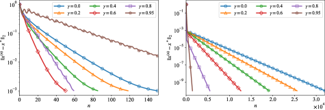
Results of the case (ii) are shown in Fig.4. In this case, $\nabla^{2}R_{m}(x^{*})$ is much more ill-conditioned compared with the case (i) since the condition number $\kappa^{*}$ is 39904.29. Due to the ill-condition, we have to choose a smaller step size $\beta=10^{-5}$ and select LOBPCG as the eigenvector solver. Meanwhile, $x^{*}$ becomes an index-5 saddle point. All these settings make the case (ii) more challenging. We observe from Fig.4 that the convergence rate of the HiSD method is very slow, while the momentum term helps to release the problem by introducing the historical gradient information. For instance, A-HiSD with $\gamma=0.95$ attains the stop criterion $\|x^{(n)}-x^{*}\|_{2}\leq 10^{-5}$ within only 6000 iterations. Furthermore, as discussed in our numerical analysis, larger $\gamma$ should be applied in ill-conditioned cases, which is consistent with the numerical observations.

5.3 Modified strictly convex 2 function

We compare the performance of A-HiSD method with another commonly-used acceleration strategy, i.e. the HiSD with the Barzilai-Borwein (BB) step size barzilai1988two , which could accelerate the HiSD according to experiment results in zhang2016optimization ; yin2019high . We apply the modified strictly convex 2 function, a typical optimization test example proposed in raydan1997barzilai

S(x)=\sum_{i=1}^{d}s_{i}a_{i}(e^{x_{i}}-x_{i})/10,

(29)

where $a_{i}=1+5(i-1)$ for $1\leq i\leq d$ , $s_{i}=-1$ for $1\leq i\leq k$ and $s_{j}=1$ for $k+1\leq j\leq d$ . $x^{*}=[0,...,0]$ is an index- $k$ saddle point of $S(x)$ . In our experiment, we set $d=100$ and $k=5$ .

We implement A-HiSD method with different momentum parameters $\gamma$ and compare with the HiSD with the BB step size $\beta_{n}$ in each iteration

\beta_{n}=\min\left\{\frac{\tau}{\|\nabla S(x^{(n)})\|_{2}},\frac{{\Delta x^{(n)}}^{\top}\Delta g^{(n)}}{\|\Delta g^{(n)}\|_{2}^{2}}\right\},

(30)

where $\Delta x^{(n)}=x^{(n)}-x^{(n-1)}$ . $\Delta g^{(n)}=\nabla S(x^{(n)})-\nabla S(x^{(n-1)})$ and $\tau=0.5$ to avoid the too large step size. SIRQIT is selected as the eigenvector solver. The initial point $x^{(0)}$ is set as $[-6,...,-6]$ .

As shown in Fig.5, the HiSD with the BB step size diverges within a few iterations, while the A-HiSD method still converges. Meanwhile, as we increase $\gamma$ , the empirical convergence rate of the A-HiSD increases, which substantiates the effectiveness and the stability of the A-HiSD method in comparison with the HiSD with the BB step size.

5.4 Loss function of neural network

We implement an interesting, high-dimensional example of searching saddle points on the neural network loss landscape. Due to the non-convex nature of loss function, multiple local minima and saddle points are main concerns of the neural network optimization dauphin2014identifying . Recent research indicates that gradient-based optimization methods with small initializations can induce a phenomenon known as ’saddle-to-saddle’ training process in various neural network architectures, including linear networks and diagonal linear networks NEURIPS2022_7eeb9af3 ; jacot2021saddle ; pesme2023saddle . In this process, network parameters may become temporarily stuck before rapidly transitioning to acquire new features. Additionally, empirical evidence suggests that vanilla stochastic gradient methods can converge to saddle points when dealing with class-imbalanced datasets—common occurrences in real-world datasets NEURIPS2022_8f4d70db . Consequently, it is urgent to figure out the impact of saddle points in deep learning. Analyzing saddle point via computations can provide valuable insights into specific scenarios.

Because of the overparameterization of neural networks, most critical points of the loss function are highly degenerate, which contains many zero eigenvalues. This challenges saddle searching algorithms since it usually leads to the slow convergence rate in practice. Let $\{(x_{i},y_{i})\}_{i=1}^{m}$ with $x_{i}\in\mathbb{R}^{d_{x}}$ and $y_{i}\in\mathbb{R}^{d_{y}}$ be the training data. We consider a fully-connected linear neural network of depth $H$

f_{linear}(\textbf{W};x)=W_{H}W_{H-1}\cdots W_{2}W_{1}x,

(31)

where $\textbf{W}=[W_{1},W_{2},...,W_{H}]$ with weight parameters $W_{i+1}\in\mathbb{R}^{d_{i+1}\times d_{i}}$ for $0\leq i\leq H-1$ with $d_{0}=d_{x}$ and $d_{H}=d_{y}$ . The corresponding empirical loss $L$ is defined by Ach

L(\textbf{W})=\sum_{i=1}^{m}\|f_{linear}(\textbf{W};x_{i})-y_{i}\|_{2}^{2}=\|W_{H}W_{H-1}\cdots W_{2}W_{1}X-Y\|_{F}^{2}.

(32)

where $X=[x_{1},...,x_{m}]$ and $Y=[y_{1},...,y_{m}]$ . In practice we could vectorize $W_{1},\cdots,W_{H}$ row by row such that $L$ can be regarded as a function defined in $\mathbb{R}^{D}$ with $D=\sum_{i=0}^{H-1}d_{i}d_{i+1}$ . According to Ach , $L$ contains a large amount of saddle points, which can be parameterzied by the data set $\{(x_{i},y_{i})\}_{i=1}^{m}$ . For instance, if $d_{i}=d_{0}$ for $1\leq i\leq H-1$ , then $\textbf{W}^{*}:=[W_{1}^{*},\ldots,W_{H}^{*}]$ is a saddle point where

W_{1}^{*}=\begin{bmatrix}U_{\mathcal{S}}^{\top}\Sigma_{YX}\Sigma_{XX}^{-1}\\ 0\end{bmatrix},\quad W_{h}^{*}=I\text{ for }2\leq h\leq H-1,\text{ and }W_{H}^{*}=\begin{bmatrix}U_{\mathcal{S}}&0\end{bmatrix}.

(33)

Here $I$ is the identity matrix, $\mathcal{S}$ is an index subset of $\{1,2,...,r_{\max}\}$ for $r_{\max}=\min\{d_{0},...,d_{H}\}$ , $\Sigma_{XX}=XX^{\top}$ , $\Sigma_{YX}=YX^{\top}$ , $\Sigma=\Sigma_{YX}\Sigma_{XX}^{-1}\Sigma_{YX}^{\top}$ and $U$ satisfies $\Sigma=U\Lambda U^{\top}$ with $\Lambda=\text{diag}(\lambda_{1},...,\lambda_{d_{y}})$ . It is assumed in Ach that $\lambda_{1}>...>\lambda_{d_{y}}>0$ , which holds true under the data of this experiment. $U_{\text{S}}$ is then obtained by concatenating column vectors of $U$ according to the index set $\mathcal{S}$ .

In this experiments, we set the depth $H=5$ , the input dimension $d_{x}=10$ , the output dimension $d_{y}=4$ , $d_{i}=10$ for $1\leq i\leq 4$ , and the number of data points $m=100$ . Data points $(x_{i},y_{i})$ are drawn from the normal distributions $\mathcal{N}(0,I_{d_{x}})$ and $\mathcal{N}(0,I_{d_{y}})$ , respectively. The initial point is $(W_{1}^{(0)},\cdots,W_{H}^{(0)})=\textbf{W}^{*}+(V_{1},\cdots,V_{H})$ where $(V_{1},\cdots,V_{H})$ is a random perturbation whose elements $(V_{h})_{i,j}$ are drawn from $\mathcal{N}(0,\sigma^{2}_{h})$ independently, with $\sigma_{h}=0.5\frac{\|W_{h}^{*}\|_{F}}{\sqrt{d_{h-1}d_{h}}}$ . Under the current setting, $\textbf{W}^{*}$ is a degenerate saddle point with 16 negative eigenvalues and several zero eigenvalues. Although A-HiSD is developed under the framework of non-degenerate saddle points, we show that this algorithm works well for the degenerate case. We set the step size $\beta=0.1$ and the LOBPCG is selected as the eigenvector solver. Due to the highly degenerate property of the loss landscape, $\textbf{W}^{*}$ is not an isolated saddle point but lies on a low-dimensional manifold. Hence we compute the gradient norm instead of the Euclidean distance as the accuracy measure.

From Fig.6 we find that the A-HiSD with $\gamma=0.9$ attains the tolerance $10^{-7}$ within 500 iterations, while that the HiSD (i.e. the case $\gamma=0$ ) takes about 5000 iterations. In Table 1, we report the number of iterations (denoted as ITER) and the computing time in seconds (denoted as CPU) of the the problem in details for the comparison. A faster convergence rate is achieved as we gradually increase $\gamma$ , which indicates the great potential of A-HiSD method on the acceleration of convergence in highly degenerate problems.

Table 1: The ITER and CPU of HiSD (

\gamma=0

) and A-HiSD (with

\gamma=0.3,0.6,0.9

) for searching degenerate index-16 saddle points of the loss function of the linear neural networks. The speedup equals to (CPU of HiSD)/(CPU of A-HiSD).

$\gamma=0$		$\gamma=0.3$			$\gamma=0.6$			$\gamma=0.9$
CPU	ITER	CPU	ITER	speedup	CPU	ITER	speedup	CPU	ITER	speedup
56.22	4830	41.80	3376	1.33	25.77	1917	2.15	6.62	382	8.35

6 Concluding remarks

We present the A-HiSD method, which integrates the heavy ball method with the HiSD method to accelerate the computation of saddle points. By employing the straightforward update formulation from the heavy ball method, the A-HiSD method achieves significant accelerations on various ill-conditioned problems without much extra computational cost. We establish the theoretical basis for A-HiSD at both continuous and discrete levels. Specifically, we prove the linear stability theory for continuous A-HiSD and rigorously prove the faster local linear convergence rate of the discrete A-HiSD in comparison with the HiSD method. These theoretical findings provides strong supports for the convergence and acceleration capabilities of the proposed method.

While we consider the A-HiSD method for the finite-dimensional gradient system in this paper, it has the potential to be extended to investigate the non-gradient systems, which frequently appear in chemical and biological systems such as gene regulatory networks QIAO2019271 . Furthermore, this method can be adopted to enhance the efficiency of saddle point search for infinite-dimensional systems, such as the Landau-de Gennes free energy in liquid crystals han2021solution ; Shi_2023 . Lastly, the effective combination of HiSD and the heavy ball method inspires the integration of other acceleration strategies with HiSD, such as the Nesterov accelerated gradient method nesterov1983method and the Anderson mixing anderson1965iterative . We will investigate this interesting topic in the near future.

Funding This work was supported by National Natural Science Foundation of China (No.12225102, T2321001, 12050002, 12288101 and 12301555), and the Taishan Scholars Program of Shandong Province.

Data Availability The datasets generated and/or analysed during the current study are available from the corresponding author on reasonable request

Declarations

Conflict of interest The authors have no relevant financial interest to disclose.

References

(1) Achour, E.M., Malgouyres, F., Gerchinovitz, S.: The loss landscape of deep linear neural networks: a second-order analysis (2022)
(2) Anderson, D.G.: Iterative procedures for nonlinear integral equations. J. ACM 12(4), 547–560 (1965)
(3) Barzilai, J., Borwein, J.M.: Two-point step size gradient methods. IMA J. Numer. Anal. 8(1), 141–148 (1988)
(4) Bonfanti, S., Kob, W.: Methods to locate saddle points in complex landscapes. J. Chem. Phys. 147(20) (2017). URL 204104
(5) Boursier, E., PILLAUD-VIVIEN, L., Flammarion, N.: Gradient flow dynamics of shallow relu networks for square loss and orthogonal inputs. In: Advances in Neural Information Processing Systems, vol. 35, pp. 20105–20118. Curran Associates, Inc. (2022)
(6) Burton, R.E., Huang, G.S., Daugherty, M.A., Calderone, T.L., Oas, T.G.: The energy landscape of a fast-folding protein mapped by Ala → Gly substitutions. Nat. Struct. Mol. Biol. 4(4), 305–310 (1997)
(7) Cai, Y., Cheng, L.: Single-root networks for describing the potential energy surface of Lennard-Jones clusters. J. Chem. Phys. 149(8) (2018). URL 084102
(8) Cancès, E., Legoll, F., Marinica, M.C., Minoukadeh, K., Willaime, F.: Some improvements of the activation-relaxation technique method for finding transition pathways on potential energy surfaces. J. Chem. Phys. 130(11) (2009). URL 114711
(9) Cerjan, C.J., Miller, W.H.: On finding transition states. J. Chem. Phys. 75(6), 2800–2806 (1981)
(10) Cheng, X., Lin, L., E, W., Zhang, P., Shi, A.C.: Nucleation of ordered phases in block copolymers. Phys. Rev. Lett. 104 (2010). URL 148301
(11) Dauphin, Y.N., Pascanu, R., Gulcehre, C., Cho, K., Ganguli, S., Bengio, Y.: Identifying and attacking the saddle point problem in high-dimensional non-convex optimization. In: Advances in Neural Information Processing Systems, vol. 27. Curran Associates, Inc. (2014)
(12) Dauphin, Y.N., Pascanu, R., Gulcehre, C., Cho, K., Ganguli, S., Bengio, Y.: Identifying and attacking the saddle point problem in high-dimensional non-convex optimization. NeurIPS 27 (2014)
(13) E, W., Ren, W., Vanden-Eijnden, E.: Simplified and improved string method for computing the minimum energy paths in barrier-crossing events. J. Chem. Phys. 126(16) (2007). URL 164103
(14) E, W., Zhou, X.: The gentlest ascent dynamics. Nonlinearity 24(6) (2011). URL 1831
(15) Fukumizu, K., Yamaguchi, S., Mototake, Y.i., Tanaka, M.: Semi-flat minima and saddle points by embedding neural networks to overparameterization. In: Advances in Neural Information Processing Systems, vol. 32. Curran Associates, Inc. (2019)
(16) Gao, W., Leng, J., Zhou, X.: An iterative minimization formulation for saddle point search. SIAM J. Numer. Anal. 53(4), 1786–1805 (2015)
(17) Gould, N., Ortner, C., Packwood, D.: A dimer-type saddle search algorithm with preconditioning and linesearch. Math. Comp. 85(302), 2939–2966 (2016)
(18) Gu, S., Zhou, X.: Simplified gentlest ascent dynamics for saddle points in non-gradient systems. Chaos 28(12) (2018). DOI 10.1063/1.5046819. URL 123106
(19) Han, Y., Hu, Y., Zhang, P., Zhang, L.: Transition pathways between defect patterns in confined nematic liquid crystals. J. Comput. Phys. 396, 1–11 (2019)
(20) Han, Y., Yin, J., Hu, Y., Majumdar, A., Zhang, L.: Solution landscapes of the simplified Ericksen–Leslie model and its comparison with the reduced Landau–de Gennes model. Proc. R. Soc. A. 477(2253) (2021). URL 20210458
(21) Han, Y., Yin, J., Zhang, P., Majumdar, A., Zhang, L.: Solution landscape of a reduced Landau–de Gennes model on a hexagon. Nonlinearity 34(4), 2048–2069 (2021)
(22) Henkelman, G., Jónsson, H.: A dimer method for finding saddle points on high dimensional potential surfaces using only first derivatives. J. Chem. Phys. 111(15), 7010–7022 (1999)
(23) Henkelman, G., Jónsson, H.: Improved tangent estimate in the nudged elastic band method for finding minimum energy paths and saddle points. J. Chem. Phys. 113(22), 9978–9985 (2000)
(24) Jacot, A., Ged, F., Şimşek, B., Hongler, C., Gabriel, F.: Saddle-to-saddle dynamics in deep linear networks: Small initialization training, symmetry, and sparsity (2021)
(25) Kingma, D.P., Ba, J.: Adam: A method for stochastic optimization (2014)
(26) Knyazev, A.V.: Toward the preconditioned eigensolver: Locally optimal block preconditioned conjugate gradient method. SIAM J. Sci. Comput. 23(2), 517–541 (2001)
(27) Li, Y., Zhou, J.: A minimax method for finding multiple critical points and its applications to semilinear PDEs. SIAM J. Sci. Comput. 23(3), 840–865 (2001)
(28) Longsine, D.E., McCormick, S.F.: Simultaneous Rayleigh-quotient minimization methods for $Ax=\lambda Bx$ . Lin. Alg. Appl. 34, 195–234 (1980)
(29) Luo, L., Xiong, Y., Liu, Y., Sun, X.: Adaptive gradient methods with dynamic bound of learning rate. In: Proceedings of the 7th International Conference on Learning Representations. New Orleans, Louisiana (2019)
(30) Luo, Y., Zheng, X., Cheng, X., Zhang, L.: Convergence analysis of discrete high-index saddle dynamics. SIAM J. Numer. Anal. 60(5), 2731–2750 (2022)
(31) Milnor, J.: Morse theory.(AM-51), vol. 51. Princeton university press (2016)
(32) Nesterov, Y.: Introductory Lectures on Convex Optimization: A Basic Course, vol. 87. Springer Science & Business Media (2003)
(33) Nesterov, Y.E.: A method for solving the convex programming problem with convergence rate $O(1/k^{2})$ . Sov. math. Dokl. 269, 543–547 (1983)
(34) Nguyen, N.C., Fernandez, P., Freund, R.M., Peraire, J.: Accelerated residual methods for the iterative solution of systems of equations. SIAM J. Sci. Comput. 40(5), A3157–A3179 (2018)
(35) Pesme, S., Flammarion, N.: Saddle-to-saddle dynamics in diagonal linear networks (2023)
(36) Polyak, B.T.: Some methods of speeding up the convergence of iteration methods. USSR Comput. Math. Math. Phys. 4(5), 1–17 (1964)
(37) Qiao, L., Zhao, W., Tang, C., Nie, Q., Zhang, L.: Network topologies that can achieve dual function of adaptation and noise attenuation. Cell Syst. 9(3), 271–285.e7 (2019)
(38) Quapp, W., Bofill, J.M.: Locating saddle points of any index on potential energy surfaces by the generalized gentlest ascent dynamics. Theor. Chem. Acc. 133(8), 1510 (2014)
(39) Rangwani, H., Aithal, S.K., Mishra, M., R, V.B.: Escaping saddle points for effective generalization on class-imbalanced data. In: Advances in Neural Information Processing Systems, vol. 35, pp. 22791–22805. Curran Associates, Inc. (2022)
(40) Raydan, M.: The Barzilai and Borwein gradient method for the large scale unconstrained minimization problem. SIAM J. Optim. 7(1), 26–33 (1997)
(41) Reddi, S.J., Kale, S., Kumar, S.: On the convergence of Adam and beyond (2019)
(42) Samanta, A., Tuckerman, M.E., Yu, T.Q., E, W.: Microscopic mechanisms of equilibrium melting of a solid. Science 346(6210), 729–732 (2014)
(43) Shi, B., Han, Y., Yin, J., Majumdar, A., Zhang, L.: Hierarchies of critical points of a landau-de gennes free energy on three-dimensional cuboids. Nonlinearity 36(5), 2631 (2023). DOI 10.1088/1361-6544/acc62d
(44) Shi, B., Han, Y., Yin, J., Majumdar, A., Zhang, L.: Hierarchies of critical points of a Landau-de Gennes free energy on three-dimensional cuboids. Nonlinearity 36(5), 2631–2654 (2023)
(45) Stewart, G.W., Sun, J.g.: Matrix perturbation theory. Academic Press, San Diego (1990)
(46) Wales, D.: Energy Landscapes: Applications to Clusters, Biomolecules and Glasses. Cambridge University Press, Cambridge, UK (2003)
(47) Wales, D.J., Doye, J.P.: Global optimization by basin-hopping and the lowest energy structures of Lennard-Jones clusters containing up to 110 atoms. J. Phys. Chem. A 101(28), 5111–5116 (1997)
(48) Wang, J.K., Lin, C.H., Abernethy, J.D.: A modular analysis of provable acceleration via Polyak’s momentum: Training a wide ReLU network and a deep linear network. In: International Conference on Machine Learning, pp. 10816–10827. PMLR (2021)
(49) Wang, W., Zhang, L., Zhang, P.: Modeling and computation of liquid crystals. Acta Numer. 30, 765–851 (2021)
(50) Wang, Y., Li, J.: Phase field modeling of defects and deformation. Acta Mater. 58(4), 1212–1235 (2010)
(51) Xu, Z., Han, Y., Yin, J., Yu, B., Nishiura, Y., Zhang, L.: Solution landscapes of the diblock copolymer-homopolymer model under two-dimensional confinement. Phys. Rev. E 104, 014505 (2021)
(52) Yin, J., Huang, Z., Cai, Y., Du, Q., Zhang, L.: Revealing excited states of rotational bose-einstein condensates (2023)
(53) Yin, J., Huang, Z., Zhang, L.: Constrained high-index saddle dynamics for the solution landscape with equality constraints. J. Sci. Comput. 91(2) (2022). URL 62
(54) Yin, J., Jiang, K., Shi, A.C., Zhang, P., Zhang, L.: Transition pathways connecting crystals and quasicrystals. Proc. Natl. Acad. Sci. U.S.A. 118(49) (2021). URL e2106230118
(55) Yin, J., Wang, Y., Chen, J.Z., Zhang, P., Zhang, L.: Construction of a pathway map on a complicated energy landscape. Phys. Rev. Lett. 124(9) (2020). URL 090601
(56) Yin, J., Yu, B., Zhang, L.: Searching the solution landscape by generalized high-index saddle dynamics. Sci. China Math. 64(8), 1801–1816 (2021)
(57) Yin, J., Zhang, L., Zhang, P.: High-index optimization-based shrinking dimer method for finding high-index saddle points. SIAM J. Sci. Comput. 41(6), A3576–A3595 (2019)
(58) Yin, J., Zhang, L., Zhang, P.: Solution landscape of the Onsager model identifies non-axisymmetric critical points. Phys. D: Nonlinear Phenom. 430 (2022). URL 133081
(59) Yu, Y., Wang, T., Samworth, R.J.: A useful variant of the Davis–Kahan theorem for statisticians. Biometrika 102(2), 315–323 (2014). DOI 10.1093/biomet/asv008
(60) Zhang, J., Du, Q.: Shrinking dimer dynamics and its applications to saddle point search. SIAM J. Numer. Anal. 50(4), 1899–1921 (2012)
(61) Zhang, L.: Construction of solution landscapes for complex systems. Mathematica Numerica Sinica 45(3), 267–283 (2023)
(62) Zhang, L., Chen, L.Q., Du, Q.: Morphology of critical nuclei in solid-state phase transformations. Phys. Rev. Lett. 98 (2007). URL 265703
(63) Zhang, L., Du, Q., Zheng, Z.: Optimization-based shrinking dimer method for finding transition states. SIAM J. Sci. Comput. 38(1), A528–A544 (2016)
(64) Zhang, L., Zhang, P., Zheng, X.: Error estimates for Euler discretization of high-index saddle dynamics. SIAM J. Numer. Anal. 60(5), 2925–2944 (2022)
(65) Zhang, L., Zhang, P., Zheng, X.: Discretization and index-robust error analysis for constrained high-index saddle dynamics on the high-dimensional sphere. Sci. China Math. 66(10), 2347–2360 (2023)
(66) Zhang, Y., Zhang, Z., Luo, T., Xu, Z.J.: Embedding principle of loss landscape of deep neural networks. In: Advances in Neural Information Processing Systems, vol. 34, pp. 14848–14859. Curran Associates, Inc. (2021)

$\displaystyle\\|B_{n}-\tilde{A}_{n}\\|_{2}$	$\displaystyle=\\|\nabla^{2}E(x^{})-\int_{0}^{1}\nabla^{2}E(x^{}+t(x^{(n)}-x^{*}))dt\\|_{2}$	(20)
	$\displaystyle{\leq}\int_{0}^{1}\\|\nabla^{2}E(x^{})-\nabla^{2}E(x^{}+t(x^{(n)}-x^{*}))\\|_{2}dt$
	$\displaystyle{\leq}\int_{0}^{1}tdtM\\|x^{(n)}-x^{}\\|_{2}=\frac{M}{2}\\|x^{(n)}-x^{}\\|_{2},$

	$\displaystyle\Big{\\|}\sum_{j=0}^{m}T^{m-j}P_{j}\Big{\\|}_{2}$	$\displaystyle{\leq}\sum_{j=0}^{m}KC_{1}\beta(\sqrt{\gamma})^{m-j}\\|F_{j}\\|_{2}^{2}$		(27)
		$\displaystyle{\leq}2\beta K^{2}C_{1}\hat{r}\sum_{j=0}^{m}(\sqrt{\gamma})^{m-j}\theta^{j}\\|F_{0}\\|_{2}{\leq}\frac{2\beta KC_{1}\hat{r}}{\theta-\sqrt{\gamma}}\cdot K\theta^{m+1}\\|F_{0}\\|_{2}{\leq}K\theta^{m+1}\\|F_{0}\\|_{2},$		(27)