11email: {dennis.Chen, li.g, minkow, 628628}@sjtu.edu.cn22institutetext: Delphinus Lab., Sydney, 43017-6221, Australia
[email protected]
AC4: Algebraic Computation Checker for Circuit Constraints in Zero-Knowledge Proofs
Abstract
Zero-knowledge proof (ZKP) systems have surged attention and held a fundamental role in contemporary cryptography. Zero-knowledge succinct non-interactive argument of knowledge (zk-SNARK) protocols dominate the ZKP usage, implemented through arithmetic circuit programming paradigm. However, underconstrained or overconstrained circuits may lead to bugs. The former refers to circuits that lack the necessary constraints, resulting in unexpected solutions and causing the verifier to accept a bogus witness, and the latter refers to circuits that are constrained excessively, resulting in lacking necessary solutions and causing the verifier to accept no witness. This paper introduces a novel approach for pinpointing two distinct types of bugs in ZKP circuits. The method involves encoding the arithmetic circuit constraints to polynomial equation systems and solving them over finite fields by the computer algebra system. The classification of verification results is refined, greatly enhancing the expressive power of the system. A tool, AC4, is proposed to represent the implementation of the method. Experiments show that AC4 demonstrates a increase in the checked ratio, showing a 29% improvement over Picus, a checker for Circom circuits, and a 10% improvement over halo2-analyzer, a checker for halo2 circuits. Within a solvable range, the checking time has also exhibited noticeable improvement, demonstrating a magnitude increase compared to previous efforts.
Keywords:
zero-knowledge proofscircuit constraintsunderconstrainedoverconstrainedalgebraic computation checker1 Introduction
Zero-knowledge proof (ZKP) systems have long occupied a fundamental position in contemporary cryptography, ever since their inception [27]. They are significantly utilized in security-sensitive applications, such as smart contracts [53], blockchain confidential transactions [53, 28], and digital currency [60], given their capacity to bolster security and privacy. ZKP systems’ potency lies in their ability to prove anything that an interactive proof system can, but without revealing any knowledge [33, 10]. Therefore, these systems have assumed the role of a potent tool enabling trust and authentication while safeguarding sensitive information.
Developers frequently choose the zero-knowledge succinct non-interactive argument of knowledge (zk-SNARK) [12] protocol for its efficiency in setting up and proving within a zero-knowledge proof (ZKP) system. Additionally, they adopt arithmetic circuits [48] as the programming paradigm due to their simplicity in representing computational problems. Both Circom and halo2 are built upon this protocol and programming paradigm. To illustrate this, consider the process of declaring a boolean value in circuit programs. In high-level languages, a boolean value can be declared directly. However, in circuit languages, a constraint must be explicitly defined to limit its possible values. For instance, the constraint ensures that can only be 0 or 1. This transformation cannot be automatically performed by existing comilers or libraries, necessitating that developers express computations using polynomial equations.
The limitation of polynomial constraint systems gives rise to two problems. The first problem is the underconstrained problem [46], which occurs when multiple outputs can fulfill the same system of equations with identical input values. This situation arises when the system of polynomial equations does not yield a mathematical function on the finite field, rendering the circuit underconstrained. As a result, malicious users could generate fake witnesses, deceive the verifier, and potentially steal the cryptocurrency [4, 19]. The second one is the overconstrained problem [46], which occurs when no outputs can satisfy the system of polynomial equations or the constraint system is inconsistent for a given input. This issue can result in a non-functional circuit. Consequently, this may lead to overconstrained bugs that cause ZK-verifier servers to reject numerous legitimate requests. Such rejections could potentially trigger Distributed Denial of Service (DDoS) problems. Furthermore, it is evident that underconstrained circuits can produce more severe consequences than their overconstrained counterparts.
To this end, we conducted an investigation into the constraints on Circom or halo2 circuit programs. By reconsidering the formalization paradigm, we modeled underconstrained and overconstrained problems as algebraic inquiries. Specifically, we examined whether a system of polynomial equations over a finite field has multiple solutions. To support our motivation, we analyzed the official library of circom circuit templates provided by iden3 and collected halo2 circuit templates from . Our analysis revealed that nearly 70% of these templates are linear, and efficient algorithms exist for solving linear systems of equations. Consequently, we categorized constraint problems into diverse types based on their maximal degree. We then employed a unified arithmetic solution framework to address each type separately.
To summarize, contributions can be elaborated as follows:
-
•
We proposed a methodology that utilizes computer algebra systems to model circuit programs as polynomial systems over finite fields, with the aim of verifying their correctness.
-
•
We developed AC4, a highly efficient and practical tool that leverages the aforementioned framework to effectively handle larger circuit programs.
-
•
We constructed datasets specifically tailored for Circom and halo2 circuits. By comparing the checked ratio and checking speed of AC4 against other tools, we observed substantial improvements in both metrics.
2 Background
Zk-SNARKs. Non-interactive ZKP protocols, such as zk-SNARKs [11], allow verifiers to be assured of a statement’s truth without gaining any knowledge beyond its validity [27]. Blum et al. demonstrated that computational zero-knowledge can be achieved without interaction by sharing a common random string between the prover and the verifier [15, 58]. The non-interactive protocol conveys the proof through a message from the prover to the verifier, ensuring efficiency. zk-SNARKs reign supreme in ZKP systems due to lightning-fast verification of even large programs, using tiny proofs (mere hundreds of bytes) within milliseconds.
Arithmetic Circuits. Arithmetic circuits, fundamental models for polynomial computation in complexity theory, process variables/numbers using addition and multiplication. Conceptually, arithmetic circuits offer a formal method for understanding the complexity of computing polynomials. Note that all variables mentioned in arithmetic circuits represent signals in the Circom language.
Definition 1 (Arithmetic circuit [55])
An arithmetic circuit in the variables over the field is a labelled directed acyclic graph. The inputs are assigned by variables from or by constants. The internal nodes act as computational operations that add or multiply to calculate the sum or product of the polynomials on the tails of incoming edges. The output of a circuit is the polynomial computed at the output node.
Circuit Languages. The growing field of ZKPs has led to the development of specialized circuit languages designed to create and manage the underlying circuits needed for these proofs. Two notable examples are the Circom [9] and halo2 [59] frameworks.
Circom is a domain-specific language that leverages SNARK technology and employs arithmetic circuits as its programming paradigm. Programmers define circuits using specific operators: for equality checks, or for signal assignment, and or for simultaneous assignment. These circuits conform to the rank-1 constraint system (R1CS) format. The R1CS format is expressed as , where , , and are linear combinations of signals. After compiling the circuit into R1CS format and computing a witness using the input, the snarkjs tool can be employed to generate and verify a ZKP for the specified input.
Halo2 provides a more flexible and scalable method for constructing ZKPs. It employs PLONKish arithmetization [26], which supports recursive proof composition, thereby enhancing scalability. In halo2, circuits are built using polynomials and lookups. This construction allows for more efficient proof generation and verification.
It is reasonable to conclude that arithmetic circuits in both circom and halo2 can be treated as sets of polynomial equations, despite differing in their representations, methods of construction, and evaluation. In particular, halo2 supports constraints that are typically quadratic or higher. The specific implementation and optimization goals determine the exact nature of these constraints. We address circuit constraint verification by extending arithmetic circuit definitions with constraints.
Definition 2 (Constraint in Circom)
A constraint is a quadratic equation over a finite field :
where are coefficient vectors over , is a vector of variables over , and the cross product means the product of 2 scalars .
A halo2 circuit constraint is more general.
Definition 3 (Constraint in halo2)
A constraint in halo2 is a polynomial equation over a finite field :
where is the degree of the constraint, are the coefficient scalars, and are the variables.
Definition 4 (Arithmetic circuit with constraints)
An arithmetic circuit with constraint with constraints can be defined as a tuple , where is an arithmetic circuit on variable set . is the union of two disjoint sets and , where represents known input variables, and represents unknown variables including the non-constant variables including temporal variables and output variables . includes all the constraints of .
Computer algebra. Computer algebra [16] revolves around the manipulation of algebraic expressions and various mathematical entities. This field has spurred the creation of computer algebra systems capable of autonomously tackling a broad spectrum of theoretical and practical mathematical challenges. A contemporary computer algebra system boasts a diverse array of functionalities, encompassing Gröbner bases, cylindrical algebraic decomposition, lattice basis reduction, linear system solving, arbitrary and high-precision arithmetic, interval arithmetic, linear and nonlinear optimization, Fourier transforms, Diophantine equation solving, among others. These capabilities are indispensable for both theoretical investigations and practical applications.
Gröbner basis. A Gröbner basis is a set of multivariate polynomials that has desirable algorithmic properties. Every set of polynomials can be transformed into a Gröbner basis. This process generalizes three familiar techniques: Gaussian elimination for solving linear systems of equations, the Euclidean algorithm for computing the greatest common divisor of two univariate polynomials, and the Simplex algorithm for linear programming. Algorithms on Gröbner basis are widely used in mathematical and verification tools. The computation of a Gröbner basis can be performed using Buchberger’s algorithm [54], while Faugère F5 algorithm [23] is a significant improvement over the former. It introduces the concept of signatures to predict and eliminate unnecessary computations, which can potentially increase the efficiency of Gröbner basis computation.
3 Problem Statements
Detecting overconstrained or underconstrained circuits in circuit languages boils down to an algebraic inquiry into the number of solutions for a polynomial equations system over a finite field. This inherent connection naturally leads us to model circuits as such systems and leverage algebraic methods for analysis. Our method follows the classification-and-discussion scheme. Our strategy categorizes circuits by degree and applies specialized solutions within each category, leading to significant efficiency and scalability gains.
3.1 Constraint Problems
The construction of arithmetic circuits is plagued by two critical challenges: overconstrained and underconstrained circuits. Programmer-authored circuits, even from seasoned ZKP developers, often bear inadvertently miscalibrated constraints, leading to these issues. While completely eradicating these issues remains a persistent hurdle, current approaches fall short of effectiveness. This subsection tackles this double-edged sword head-on, proposing a novel approach to ensure the construction of robust and reliable arithmetic circuits.
Overconstrained bugs. As described in the work by Labs et al. [35], overconstrained circuits are unable to uphold the completeness of ZKP. A circuit program is deemed overconstrained when its corresponding polynomial constraints are overconstrained, indicating that the circuit cannot produce any valid outputs regardless of the inputs provided. This inconsistency in the constraint system for a given input characterizes the state of being overconstrained. Despite their deceptive simplicity in concept and the misconception that they are less critical than other types of attacks, denial of service (DoS) attacks are often underappreciated regarding their security implications. Notably, DoS attacks require neither high skill nor deep knowledge,, contributing to their low cost for malicious attackers as highlighted by Zcash [38].
Underconstrained bugs. Recent studies have discovered that underconstrained bugs in arithmetic circuits can lead to various security threats, including the ability for attackers to forge signatures, steal user concurrency, or create counterfeit crypto-coins. A circuit program is classified as underconstrained when the corresponding polynomial constraints are also underconstrained. This condition arises when there exists an input for which multiple distinct outputs can be produced, and the circuits are all considered valid. In essence, an underconstrained circuit program may unintentionally permit the acceptance of unwanted signals, making it susceptible to exploitation by malicious entities.
3.2 Categories of Elements
In our method, categorization is essential to account for the different types of variables in arithmetic circuits. Variables can be classified based on their source: some are determined by external inputs, while others depend on internal variables. It is also important to categorize variables according to their degree. Due to the computational complexity of verifying certain circuits, we can only provide coarse-grained results. This limitation underscores the importance of categorizing the outcomes as well.
Category of Variables. The variables in a circuit program consist of the input signals , temporary signals , and output signals . The user provides the values for , which can be regarded as known values . On the other hand, the variables in , whose values are not constant, are regarded as unknown variables within the constraints. The key issue of the constraint problem is identifying the unique characteristics of the variables.
Category of Constraints and Circuits. The constraint is an algebraic polynomial equation whose degree is under 2 over a finite field , while the circuits are a system of algebraic polynomial equations whose degree is under 2 over a finite field, with their generator variables being .
The three types of constraints to consider are precise linear equations, -coefficient linear constraints, and higher constraints. A precise linear constraint is defined by having linear generator variables with constant coefficients. Conversely, a -coefficient linear equation includes at least one generator variable with a coefficient represented by the known variables , and none of the generator variables’ coefficients are represented by the unknown variables . Lastly, a higher equation is distinguished by containing at least one generator variable with a coefficient represented by the unknown variables .
The system of constraints, namely circuits, can be categorized into three types based on the constraints outlined above: precise linear circuits, -coefficient circuits, and higher-order circuits. A precise linear circuit consists solely of precise linear constraints, while a -coefficient circuit must contain at least one -coefficient linear constraint and no higher-order constraints. Finally, a higher-order circuit should include at least one higher-order constraint.
3.3 Problem Reduction
This section demonstrates the reduction of the under/overconstrained problems of a circuit to the number of solutions of the corresponding polynomial equations.
Definition 5 (Polynomials over finite fields)
For a finite field and formal variables , denotes the set of polynomials in with coefficients in . By taking the variables to be in , a polynomial can be viewed as a function from .
To reduce the circuit constraint problems to the number of solutions of polynomials, we have the following proposition:
Proposition 1 (Circuit-Poly Reduction)
For each circuit , there exists , such that , where is a bijection function from a circuit to polynomial equations over finite fields.
A bijection can be constructed between the formal variables of polynomials and the variables of a circuit because their domain is the same finite field . The meta operator set of polynomial circuits is 111 is the complementary operation on finite fields and the meta operator set of a polynomials are , so . Because the additive group over finite fields is an Abelian group under ‘+’, the operation of shifting the terms does not change the properties of the original variables and constraints. However, a constraint of a polynomial circuit can only be constant, linear, or higher, while polynomials exceed the limit of the degree of variables. Consequently, the constraints of a polynomial circuit are a subset of polynomials.
Based on the argument above, completely checking the constraint status of circuits can be achieved by solving polynomials. More concretely, the constraint problem corresponds to figuring out the number of solutions for polynomials.
4 Methodology
4.1 AC4 Framework
Fig. 1 illustrates the overall workflow of our proposed tool, , which receives a Circom program file as the input, and compiles the program in debug mode into an R1CS format file along with a sym file. To retrieve the variables and constraints from the compiled files, a task-specific parser is implemented to handle those compiled files, focusing on unknown variables within constraints. After that, the extracted constraints are then simplified into equations. A categorizing mechanism is leveraged in Section 3.2 to determine the specific category of the circuit according to its simplified equation system. Based on the category result of circuits, three types of solvers is employed to address them respectively.
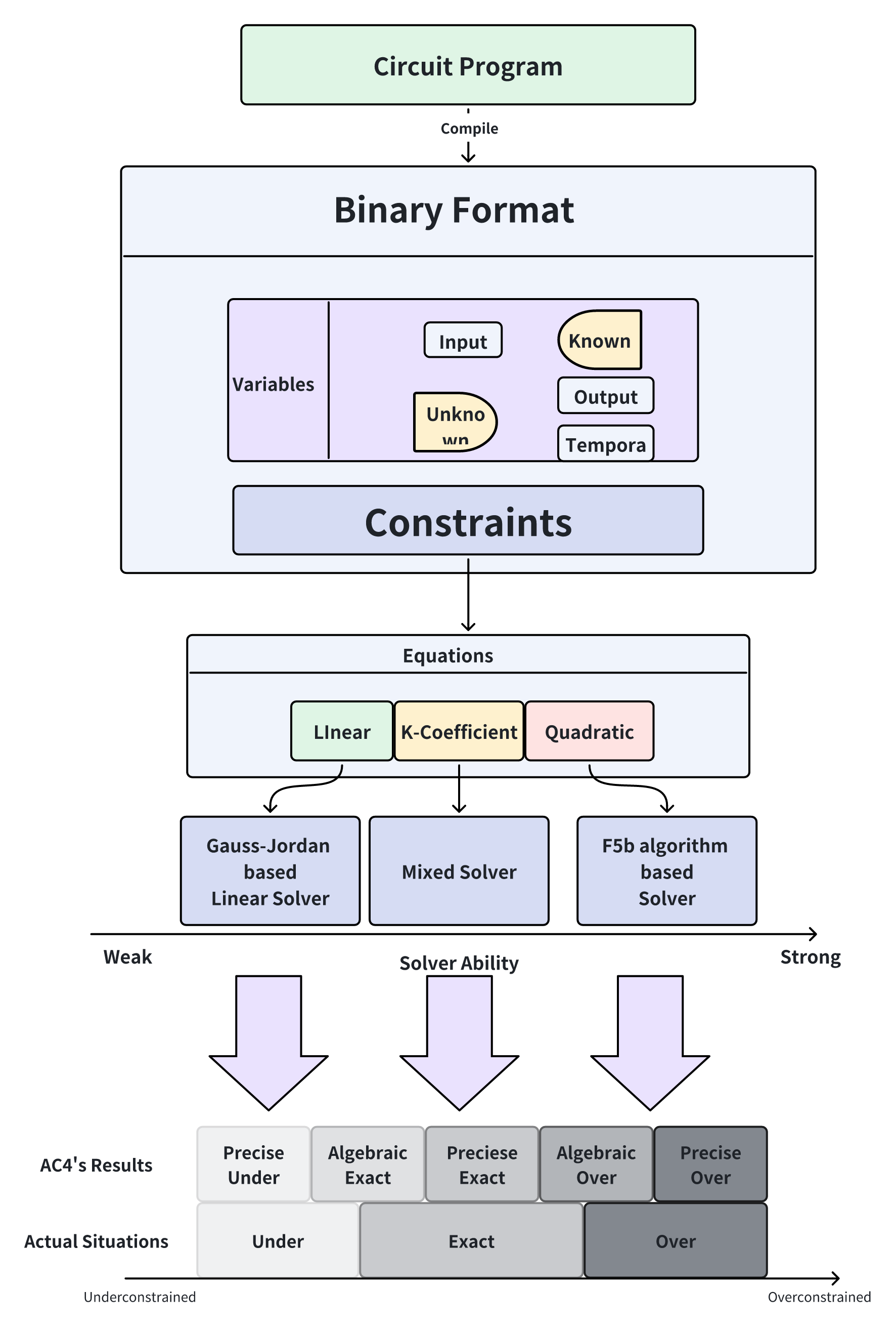
In the context of a precisely pure linear circuit, the system of linear equations can be represented in matrix form. While it may seem natural to rely on rank to determine the number of solutions, it is more important to prioritize verifying the uniqueness of the output variable set. Therefore, solving the system demands a suitable method for linear equations. Specifically, in , the Gauss-Jordan method[51] is utilized to obtain the solution of the circuits as well as to ascertain the uniqueness of the set of output variables.
The system of -coefficient linear equations corresponding to an algebraically linear circuit can be represented in matrix form. However, it is imperative to note that algebraic computation does not inherently account for the division by zero problem. Consequently, for certain specific inputs , the rank of the matrix may decrease, potentially altering the outcome of . Rank reduction risks are mitigated by strategically identifying and treating special input cases. Our approach addresses this challenge through heuristic approaches to improve the efficiency and accuracy.
For higher-order circuits, we solve the coefficients and verify if the circuit will be underconstrained with specific inputs. Then, we use to directly solve the systems of polynomial equations with Gröebner basis[18] and check the uniqueness of the output variables.
Here, an example will be used to demonstrate our workflow and enhance readers’ comprehension. The template in Fig. 2 refers to the Circom circuit Decoder, which converts a w-ary number into a one-hot encoded format.
Upon setting , the Decoder(2) emerges as a 2-bit decoder. This circuit is then transformed into a format denoted as , where the sets are defined as follows: , , , and .
Based on the classification of circuits mentioned above, it is evident that this circuit is not linear. To analyze this, we begin by treating the variable as a coefficient and proceed to solve for the undetermined coefficients of each equation. This process yields the solutions . When substituting into , the resulting equations are . Notably, can take on any value over the finite field, indicating that the circuit is underconstrained.
4.2 Adaptive Checking with Relaxation and Partial Results
AC4 is designed to provide precise results when analyzing circuits. However, when dealing with large or complex circuits, it might produce an “unknown” outcome due to the scalability. To handle these situations, AC4 relaxes its strict checking conditions and instead returns partial, but still meaningful, results.
In certain cases, the input coefficients in circuit equations can be difficult to determine as zero or non-zero. To simplify, AC4 treats all combinations of input and constant values as non-zero, allowing for a more straightforward algebraic result. For example, in an equation like , AC4 assumes the input coefficients are non-zero, so the output becomes . This yields a workable solution, even if not fully precise. Under this assumption, the overconstrained and exact-constrained results may not align with the actual situation of the circuits. We name the former as algebraic results. In contrast, by precisely, we mean that the result are directed obtained without the above assumption. Hence, as depicted in Fig. 3, AC4 generates five practical categories of results: algebraic overconstrained, precisely overconstrained, algebraic exact-constrained, precisely exact-constrained, and precisely underconstrained.
While its primary objective is to provide precise results during circuit analysis, AC4 recognizes the challenges posed by large circuits with numerous parameters. In such scenarios, where a precise result may be unattainable, AC4 adjusts its approach by relaxing the strictness of its checking conditions. This adaptability enables AC4 to yield a meaningful partial result, ensuring that even with complex circuits, users can still gain valuable insights into the circuit’s behavior.
To provide more detailed feedback on unsolvable circuits, AC4 refines its result classification. It introduces two intermediate categories, algebraic exact-constrained and algebraic overconstrained, which offer additional insights. These categories help analysts understand whether a circuit may be underconstrained (too flexible) or overconstrained (no valid solutions) by examining the algebraic structure of the equation matrix.
The relationship between AC4’s results and the actual circuit behavior is also cross-referenced with ground truth. Three categories—precisely underconstrained, precisely exact-constrained, and precisely overconstrained-directly correspond to whether a circuit is under, exact or overconstrained. However, the algebraic categories offer more nuanced information. For example, an algebraically exact-constrained circuit might be either underconstrained or exact-constrained in reality, while algebraic overconstrained cases could actually be exact-constrained or overconstrained.
Unknown results may stem from circuit size, computational complexity, or the inherent NP-hardness of solving polynomial equations over finite fields.
By relaxing the strict checking conditions, AC4 can filter out cases that are definitely under or overconstrained, providing more efficient and useful results even when a full solution isn’t possible.

4.3 Checking Circuits: Category-Based Algorithms
From above, we divide the overall circuit verification problem space into three types: precisely linear, -coefficient linear, and higher-order separately. In this section, we introduce those algorithms in detail.
Precisely linear. The majority of circuits are precisely linear, so they can be represented by a coefficient matrix and a constant vector . While it is commonly thought to use the rank of the equation matrix to determine the number of solutions, the solver’s objective is only to verify the uniqueness of output variables. In contrast, rank-reducing methods impose restrictions on the uniqueness of all variables, including temporary variables. Using the Gauss-Jordan method to get the rank of the corresponding matrix is analogous to getting the solution of the system of equations. Consequently, there is no significant difference in the time complexity. The pesudo-code is given in Algorithm
Higher-Order. A heuristic approach will be used to identify input variables that may cause the circuit to become underconstrained (shown in Algorithm3), aiming to improve accuracy and efficiency. The coefficients of the unknown variables are treated as equations and their solutions will be stored in a frequency table for counting the occurrences of each solution. Then, the solver sorts the solutions based on their frequencies and iteratively substitutes them into the original system of equations to obtain a new system, which is then solved to check if the circuit is underconstrained. If the input variable causing the circuit to become underconstrained cannot be identified, the system of equations will be directly solved with Gröbner basis to verify the constrained situation of the circuit. The pseudo-code of checking polynomial circuits is given in Algorithm2.
Although in nature, these equations are considered linear due to their higher-order terms containing one or more known variables, Hence, they are treated as linear circuits and represented in matrix form to enhance verification efficiency. For these circuits, we still use the previous heuristic approach given in Algorithm 2, to determine if there are special inputs that can cause the underconstrained condition, aiming to enhance efficiency. Afterwards, a -coefficient linear circuit can be succinctly represented by a coefficient matrix and a constant vector , and checked as a linear case. The pseudo-code of checking -coefficient circuits is given in Algorithm4.
4.4 Complexity Analysis
This section examines the time complexity associated with each category of circuits. For linear circuits, including those characterized by -coefficient linear circuits, the Gauss-Jordan elimination method has a time complexity of [3]. Our statistical analysis of Circomlib [32] indicates that the majority of cases involve linear circuits. Consequently, we anticipate that our algebraic-based method will significantly enhance performance compared to SMT solvers. In the case of higher-order circuits, we employed the algorithm, which is designed for computing Gröbner bases.[23] This algorithm typically exhibits or time complexity in the worst-case scenarios. However, the algorithm demonstrates substantial improvements over its predecessors, such as Buchberger’s algorithm[18] and the algorithm.
5 Evaluations
5.1 Environment Setting and Metrics
Environment configuration. The evaluations were performed on a machine with a 16-core AMD Ryzen 9 5950x processor and 128GB of DRAM.
Check Benchmark. We settle a representative benchmark to evaluate the effectiveness and accuracy of and Picus [46]. The benchmark was based on the data set provided by and Picus, which had been collected from Circomlib, the standard library from Circom. All cases of our benchmark were divided into two parts: Circomlib-utils benchmarks, which was extracted from the Circomlib utils library and had a smaller size, and Circomlib-core benchmarks, which was extracted from the Circomlib core library and had a larger size [46].
Furthermore, we established a benchmark to evaluate the effectiveness and accuracy of AC4 and the halo2-analyzer[31], as implemented in the study by Soureshjani et al. (2023) [52]. This benchmark was constructed using a dataset of classical halo2 circuits, which were collected from various GitHub projects.
The primary benchmark focuses on circom datasets, while our results also demonstrate improvements on halo2 datasets compared to other tools.
Benchmark Metrics Checked Ratio. The solved benchmarks are initially categorized into three types: precisely solved, algebraically solved, and unknown. The precisely solved cases are further categorized into three types: precisely exact-constrained, which means that the circuit is safe; precisely overconstrained, indicating that the circuit is overconstrained; and precisely underconstrained, which suggests that the circuit is underconstrained. We omit this metric as (Precisely Solved).
On the other hand, we propose a more relaxed metric, (Algebraic Solved), by remapping cases that failed to obtain precise results into two new categories: algebraic exact-constrained and algebraic overconstrained, to reject overconstrained and underconstrained respectively. Note that still returns unknown for extremely computationally exhausting cases.
Checking time. In this metric, our emphasis lies on the benchmark data on the parts that both and other tools can solve, and then proceed to compare the checking time of the tools.
5.2 Detailed Evaluation over Circom Circuits
The Conditions of the Data Set over Circom
The size condition. Table 1 presents the size condition of the benchmark set. Notably, within the benchmark set Core, there are three circuits with over 200,000 constraints, which are believed to be unsolvable using standard computers. Interestingly, in these three cases, only Sha256compression results in an out-of-memory exception due to the presence of around 20,000 unknown variables, resulting in the creation of a very large matrix. In contrast, the other two cases each have only one known variable, making the circuits easier to check.
| Benchmark set | # of circuits | Avg. # of expr_num | Avg. # of unknown_num | Avg. # of out_num |
|---|---|---|---|---|
| utils | 66 | 1992 | 12 | 9 |
| core | 110 | 6941 | 200 | 30 |
| total | 176 | 5085 | 130 | 22 |
We categorize circuits based on their constraint numbers in Table 2, considering those with a constraint number less than 100 as “small” circuits, those with a constraint number in the range as “medium” circuits, and those with a constraint number in the range as “large” circuits. This classification, which may be rudimentary, does not consider output signals. It is evident that small circuits can be solved directly, whereas other circuits may require specific restrictions to be solved within an acceptable time frame.
| Benchmark set | utils | core | total |
|---|---|---|---|
| small | 49 | 63 | 112 |
| medium | 8 | 24 | 32 |
| large | 9 | 23 | 32 |
The type condition. As shown in the table 4, The benchmark set comprises 176 circuits, distributed as 71.6% precisely linear, 6.2% -coefficient linear, and 22.2% quadratic, mirroring the range of circuit types encountered in real-world applications. Upon further examination of the -coefficient and quadratic cases, it becomes evident that a significant portion of them are binary circuits associated with cryptographic algorithms. Instead of exhaustive arithmetic solutions, focusing on binary optimization strategies offers promising efficiency gains in checking these circuits. For instance, the circuit Num2BitsNeg@bitify_256 is a quadratic circuit designed to convert an integer over a finite field into a 256 bit-vector, with all its unknown variables constrained by , indicating that they are strictly bits with their value limited to 0 or 1. Appropriately identifying these circuits and applying binary methods for solving them represents a more efficient approach compared to arithmetic methods.
Benchmark Results over Circom
Checking time. The checking time of the benchmark set is presented in Table 3, with a focus on the relationship between benchmark size and solving difficulty. It is observed that the larger benchmarks present greater difficulty in solving, resulting in longer solution times. However, in some large circuits, despite a high number of constraints, the number of output signals is limited to 1, allowing for a relatively easy check once the file read operation concludes. Nonetheless, there exist extremely large circuits that are characterized by a linear type, yet their extensive constraint size renders the Gaussian-Jordan method challenging to execute, leading to out-of-memory issues. Conversely, smaller cases are relatively straightforward to solve directly but due to limitations, the precise solution is not attainable, resulting in algebraic outcomes.
Fortunately, the majority of practical Circom circuits are of the precisely linear type. This characteristic is advantageous because medium or large circuits that are not precisely linear cannot be solved directly due to unknown outcomes. Therefore, alternative methods must be utilized to bypass the direct solution of non-linear circuits. Additionally, providing a more accurate range to determine whether to solve the circuits can help avoid obtaining algebraically solved results. This approach is crucial for maintaining clarity and precision in circuit analysis.
| Benchmark | Utils | Core | overall | |||||||
| Size | small | medium | large | overall | small | medium | large | overall | ||
| Avg. # variable | K | 15 | 424 | 14309 | 2014 | 36 | 435 | 24984 | 5159 | 3973 |
| U | 4 | 18 | 58 | 13 | 11 | 78 | 26 | 29 | 23 | |
| O | 2 | 2 | 57 | 9 | 10 | 78 | 26 | 29 | 21 | |
| total v | 18 | 442 | 14366 | 2026 | 47 | 512 | 25010 | 5188 | 3995 | |
| constraints | 14 | 244 | 14230 | 1993 | 17 | 474 | 24923 | 5144 | 3956 | |
| Avg. PS Time(s) | 0.57 | 0.52 | 9.06 | 1.83 | 0.42 | 2.4 | 14.59 | 3.71 | 3.03 | |
| Avg. AS&PS Time(s) | 1.26 | 2.45 | 8.33 | 2.41 | 0.40 | 2.4 | 13.47 | 3.48 | 3.06 | |
Checked Ratio. The checked ratio of the benchmark sets categorized by circuit type is presented in Table 4. The data indicates a significantly high solved ratio for precisely linear circuits. However, Substantial constraints in circuits result in very large augmented matrices. As a consequence, the solve ratio of coefficient circuits is relatively low. This is attributed to the adoption of an algebraic strategy for coefficient circuits, which in turn leads to the direct solving of small-size coefficient circuits without returning a precise result.
Heuristic algorithms initially assess potential underconstraint in quadratic circuits. We then apply classic algorithms for solving quadratic equations over finite fields to obtain direct solutions. Moreover, in the case of specific binary circuits such as BinSum and Num2Bits, a detection method is utilized to verify the boolean nature of unknown variables. Upon confirmation, a specialized method for solving binary circuits is employed in lieu of arithmetic-based approaches. Most circuits are thoroughly verified before processing.
| Benchmark | Utils | Core | overall | ||||||
| type | pl | kcl | q | overall | pl | kcl | q | overall | |
| ps_num | 45 | 3 | 7 | 55 | 75 | 3 | 23 | 101 | 156 |
| as_num | 3 | 3 | 5 | 11 | 2 | 2 | 4 | 8 | 19 |
| total_num | 48 | 6 | 12 | 66 | 77 | 5 | 27 | 109 | 175 |
| ps_rat | 94% | 60% | 58% | 83% | 96% | 60% | 85% | 91% | 89% |
| ps&as_rat | 100% | 100% | 100% | 100% | 98% | 100% | 100% | 99% | 99% |
Comparison with Baseline
In the paper [46], Picus, an implementation of the tool , is utilized for verifying the uniqueness property (under-constrained signals) of ZKP circuits. This implementation employs static program analysis and SMT solvers checking to achieve the verification of the uniqueness of ZKP circuits. Subsequently, we benchmarked the Picus program using the same benchmark set.
The completed Picus ratio for the utils benchmark set is 80.33%, for the core benchmark set it is 62.61%, and for both sets it is 69.36%. Additionally, the average solving time for the Picus solver is 425.73 seconds for the utils benchmark set, 317.88 seconds for the core benchmark set, and 365.52 seconds for both sets.


5.3 Evaluation over Halo2 Circuits
Given the current dearth of comprehensive research on halo2 circuits and the absence of template circuits provided by the official Zcash organization, we undertook the task of extracting 10 of the most frequently utilized halo2 circuit types from GitHub repositories dedicated to halo2 projects. These extractions were subsequently employed to construct a relevant dataset. Utilizing this custom-curated dataset, we conducted benchmark analyses in conjunction with the halo2-analyzer.
As shown in figure 5, AC4 demonstrates a enhancement in efficiency and accuracy compared to halo2-analyzer, exhibiting a 26.73% improvement in the verification time and 10% improvement in the checked ratio for halo2 circuits.


5.4 Evaluation Result Analysis
Table 3 illustrates a significant correlation between the size of the circuit and the time required for checking. Despite their size, large circuits keep checking times low due to two critical factors. Firstly, the predominance of linear circuits, efficiently addressed by the Gauss-Jordan solver, contributes to the efficiency in solving a majority of cases. Additionally, optimizations targeting binary cases within k-coefficient and higher-order circuits serve to further reduce the solving time despite their slightly larger size.
The checked ratio is high for precisely linear cases; however, there are some cases for which we cannot provide precisely checked results due to the lack of an algebraic solution. Special input scenarios can reduce the augmented matrix’s rank, yielding a solution. In contrast, for the -coefficient cases, the checked ratio is relatively low, even when a mixed solver is employed. This is because we did not implement certain static analysis methods to elaborate the benchmark set, which would have facilitated the checking of circuits. Conversely, the checked ratio is relatively high for quadratic cases, as most of these cases are in binary form. The detection method and optimization for binary quadratic circuits have significantly enhanced efficiency in checking these cases.
In the context of quadratic cases, Picus and halo2-analyzer employ the cvc5-ff-range solver. This solver first implements finite field theory and then utilizes Buchberger’s algorithm along with triangular decomposition to simplify polynomial equations. To address the problem, it further applies Collins’ cylindrical algebraic decomposition (CAD) [22] [43]. It is important to note that the time complexity of CAD is , which can be prohibitive in many scenarios involving large quadratic cases. Additionally, the algorithm demonstrates superior performance over modular integers in various cryptographic challenges.
AS Analysis. We point out that the cases that occur in the AS metric are worth discussing. In Core data split, cases that cannot be precisely solved consist of nearly 7% of the total amount, while this number increases to 17% in Utils data split. Our proposed AS mechanism enables our tool to investigate more detailed situations of constraints. By excluding an incorrect option among underconstrained and overconstrained, we narrow the possible status of these cases. Experimental results demonstrate that our tool offers valuable hints to almost 100% cases in both Core and Utils splits.
Failure Analysis. Picus utilized their algorithm Uniqueness Constraint Propagation to solve all the coefficient circuits. The algorithm simplifies verification/resolution by strategically assigning values to unknown variables through partial equation analysis, reducing unknowns. However, our methods forgo static analysis, limiting -coefficient case checking.
Analysis over halo2 circuits Halo2-analyzer employs cvc5-ff to verify circuit uniqueness, giving our tool an advantage in solving large-scale polynomial equation systems.
6 Related Work
Verification on ZK programs. Circomspect [14] serves as a static analyzer and linter designed for the Circom programming language. Picus [46] employs a static analysis method combined with an SMT solver. Circomspect and Picus share certain similarities with our work. However, Circomspect can only annotate a portion of underconstrained variables.
ZK circuit formalization has seen notable advancements: Shi et al. [50] proposed a data-flow-based algorithm for R1CS standardization, to enhance performance across R1CS tasks. Wen et al. [57] formalized and classified Circom vulnerabilities, introducing a CDG-based static analysis framework. CODA [37] emerged as a statically typed language for formal ZK system property specification and verification. Soureshjani et al.[52] applied abstract interpretation to examine halo2 circuit properties, on the Plonkish matrix using an SMT solver.
Research on ZK compilers with theorem proving is ongoing. Bangerter and Almeida et al.[7, 6, 2, 8], pioneered verifiable compilation using Isabelle/HOL [42]. PinocchioQ [25] verified Pinocchio[47], a C-based zk-SNARK, with Compcert [36] based on Coq [13]. Chin and Coglio et al [20, 21]. employed ACL2 [34] on Leo, while Bailey et al. [5] established formal proofs for six zk-SNARK constructions using the Lean theorem prover [41].
Algebra computation in circuit verification. Algebraic computation is a long-standing but niche endeavor in verification. Watanabe [56] utilized Gröbner Basis [24, 23] and polynomial reduction techniques to verify arithmetic circuits in computing and signal processing systems. Similarly, Lv et al. [40, 39] employed a computer-algebra-based approach for the formal verification of hardware. Scholl et al. [49] advanced this field by combining Computer Algebra with a Boolean SAT solver to verify divider circuits. In the context of Zero Knowledge Proof (ZKP) compilers, Alex et al. [45] presented a partial verification of a field-blasting compiler pass. Furthermore, Thomas et al. [30] introduced a novel automated reasoning method for determining the satisfiability of non-linear equation systems over finite fields. Additionally, Thomas et al. [29] enhanced the Yices2 SMT solver by implementing a new MCSat-based reasoning engine for finite fields.
Alex et al. [43] employed the C++ CLN library [17] to implement finite fields and utilized COCOALib’s [1] implementation of the Buchberger algorithm for preprocessing equations, subsequently applying CAD algorithm[22] to solve them and presents a new SMT solver for finite field equations that improves efficiency on cryptosystem verification tasks by using multiple simplified Gröbner bases and specialized propagation algorithms[44].
We emphasize that much of the work in this field reduces program or hardware issues to algebra. To our knowledge, we are the first to apply computer algebra methods in ZKPs.
7 Conclusion
Using an algebraic computation system, we have developed a technique for detecting zero-knowledge bugs in arithmetic circuits. This approach is designed to address issues caused by underconstrained or overconstrained arithmetic circuits. Unlike the traditional method of encoding the problem into formulas and utilizing an SMT solver, our approach leverages arithmetic computations, significantly improving efficiency. Additionally, to enhance the verification process, we have incorporated heuristic methods. Notably, our method directly analyzes arithmetic circuits and does not depend on a specific domain-specific language (DSL), making it applicable to a wide range of DSLs that support zk-SNARKs. Our implementation utilizes the open-source algebra computation system, SymPy, in a tool called . We conducted an evaluation involving 176 Circom circuits, and our approach successfully verified approximately 89% of the benchmark sets within a short timeframe.
In order to enhance the elaboration of the data set prior to direct solution, our approach will encompass adopting methods such as static program analysis. This will enable us to acquire comprehensive information about the circuits before applying our methods. Additionally, we aim to conduct extensive evaluations of commonly utilized circuits and design specialized algorithms for them. Furthermore, the use of theorem proving will be employed to demonstrate the correctness of a series of specific circuits. Ultimately, our goal is to develop or modify existing open-source computer algebra tools to tailor a solver for determining the number of solutions to a system of polynomial equations over a finite field.
References
- [1] Abbott, J., Bigatti, A.M.: Cocoalib: a c++ library for doing computations in commutative algebra. (2007), https://cocoa.dima.unige.it/cocoa/cocoalib
- [2] Almeida, J.B., Bangerter, E., Barbosa, M., Krenn, S., Sadeghi, A.R., Schneider, T.: A certifying compiler for zero-knowledge proofs of knowledge based on -protocols. In: Computer Security – ESORICS 2010. pp. 151–167. Springer Berlin Heidelberg, Berlin, Heidelberg (2010)
- [3] Andrén, D., Hellström, L., Markström, K.: On the complexity of matrix reduction over finite fields. Advances in Applied Mathematics 39(4), 428–452 (2007). https://doi.org/https://doi.org/10.1016/j.aam.2006.08.008
- [4] Aztec: Disclosure of recent vulnerabilities (2022), https://hackmd.io/@aztec-network/disclosure-of-recent-vulnerabilities
- [5] Bailey, B., Miller, A.: Formalizing soundness proofs of snarks. Cryptology ePrint Archive, Paper 2023/656 (2023), https://eprint.iacr.org/2023/656
- [6] Bangerter, E., Briner, T., Henecka, W., Krenn, S., Sadeghi, A.R., Schneider, T.: Automatic generation of sigma-protocols. In: Public Key Infrastructures, Services and Applications. pp. 67–82. Springer Berlin Heidelberg, Berlin, Heidelberg (2010)
- [7] Bangerter, E., Camenisch, J., Krenn, S., Sadeghi, A.R., Schneider, T.: Automatic generation of sound zero-knowledge protocols. Cryptology ePrint Archive, Paper 2008/471 (2008), https://eprint.iacr.org/2008/471
- [8] Bangerter, E., Krenn, S., Sadeghi, A.R., Schneider, T., Tsay, J.K.: On the design and implementation of efficient zero-knowledge proofs of knowledge. Software Performance Enhancements for Encryption and Decryption and Cryptographic Compilers–SPEED-CC 9, 12–13 (2009)
- [9] Bellés-Muñoz, M., Isabel, M., Muñoz-Tapia, J.L., Rubio, A., Baylina, J.: Circom: A circuit description language for building zero-knowledge applications. IEEE Transactions on Dependable and Secure Computing 20(6), 4733–4751 (2023). https://doi.org/10.1109/TDSC.2022.3232813
- [10] Ben-Or, M., Goldreich, O., Goldwasser, S., Håstad, J., Kilian, J., Micali, S., Rogaway, P.: Everything provable is provable in zero-knowledge. In: Advances in Cryptology — CRYPTO’ 88. pp. 37–56. Springer New York, New York, NY (1990)
- [11] Ben Sasson, E., Chiesa, A., Garman, C., Green, M., Miers, I., Tromer, E., Virza, M.: Zerocash: Decentralized anonymous payments from bitcoin. In: 2014 IEEE Symposium on Security and Privacy. pp. 459–474. IEEE, San Jose, California at The Fairmont (2014). https://doi.org/10.1109/SP.2014.36
- [12] Ben-Sasson, E., Chiesa, A., Tromer, E., Virza, M.: Succinct Non-Interactive zero knowledge for a von neumann architecture. In: 23rd USENIX Security Symposium (USENIX Security 14). pp. 781–796. USENIX Association, San Diego, CA (Aug 2014), https://www.usenix.org/conference/usenixsecurity14/technical-sessions/presentation/ben-sasson
- [13] Bertot, Y., Castéran, P.: Interactive Theorem Proving and Program Development: Coq’Art: The Calculus of Inductive Constructions, pp. 43–72. Springer Berlin Heidelberg, Berlin, Heidelberg (2004). https://doi.org/10.1007/978-3-662-07964-5
- [14] of Bits, T.: Circomspect (2023), https://github.com/trailofbits/circomspect
- [15] Blum, M., Feldman, P., Micali, S.: Non-interactive zero-knowledge and its applications. In: Proceedings of the Twentieth Annual ACM Symposium on Theory of Computing. p. 103–112. STOC ’88, Association for Computing Machinery, New York, NY, USA (1988), https://doi.org/10.1145/62212.62222
- [16] Bright, C., Kotsireas, I.S., Ganesh, V.: SAT solvers and computer algebra systems: a powerful combination for mathematics. In: Pakfetrat, T., Jourdan, G., Kontogiannis, K., Enenkel, R.F. (eds.) Proceedings of the 29th Annual International Conference on Computer Science and Software Engineering, CASCON 2019, Markham, Ontario, Canada, November 4-6, 2019. pp. 323–328. ACM (2019). https://doi.org/10.5555/3370272.3370309, https://dl.acm.org/doi/10.5555/3370272.3370309
- [17] Bruno Haible, R.B.K.: Cln - class library for numbers (2004), https://www.ginac.de/CLN/
- [18] Buchberger, B.: Bruno buchberger’s phd thesis 1965: An algorithm for finding the basis elements of the residue class ring of a zero dimensional polynomial ideal. Journal of Symbolic Computation 41(3), 475–511 (2006). https://doi.org/https://doi.org/10.1016/j.jsc.2005.09.007, logic, Mathematics and Computer Science: Interactions in honor of Bruno Buchberger (60th birthday)
- [19] Cash, T.: Tornado.cash got hacked. by us. (2019), https://tornado-cash.medium.com/tornado-cash-got-hacked-by-us-b1e012a3c9a8
- [20] Coglio, A., McCarthy, E., Smith, E., Chin, C., Gaddamadugu, P., Dellepere, M.: Compositional formal verification of zero-knowledge circuits. Cryptology ePrint Archive, Paper 2023/1278 (2023), https://eprint.iacr.org/2023/1278
- [21] Coglio, A., McCarthy, E., Smith, E.W.: Formal verification of zero-knowledge circuits. Electronic Proceedings in Theoretical Computer Science 393, 94–112 (Nov 2023). https://doi.org/10.4204/eptcs.393.9, http://dx.doi.org/10.4204/EPTCS.393.9
- [22] Collins, G.E.: Quantifier elimination for real closed fields by cylindrical algebraic decompostion. In: Brakhage, H. (ed.) Automata Theory and Formal Languages. pp. 134–183. Springer Berlin Heidelberg, Berlin, Heidelberg (1975)
- [23] Faugère, J.C.: A new efficient algorithm for computing gröbner bases without reduction to zero (f5). In: Proceedings of the 2002 International Symposium on Symbolic and Algebraic Computation. p. 75–83. ISSAC ’02, Association for Computing Machinery, New York, NY, USA (2002), https://doi.org/10.1145/780506.780516
- [24] Faugére, J.C.: A new efficient algorithm for computing gröbner bases (f4). Journal of Pure and Applied Algebra 139(1), 61–88 (1999). https://doi.org/https://doi.org/10.1016/S0022-4049(99)00005-5
- [25] Fournet, C., Keller, C., Laporte, V.: A certified compiler for verifiable computing. In: 2016 IEEE 29th Computer Security Foundations Symposium (CSF). pp. 268–280. IEEE, Lisboa, PORTUGAL (2016). https://doi.org/10.1109/CSF.2016.26
- [26] Gabizon, A., Williamson, Z.J., Ciobotaru, O.: Plonk: Permutations over lagrange-bases for oecumenical noninteractive arguments of knowledge. Cryptology ePrint Archive, Paper 2019/953 (2019), https://eprint.iacr.org/2019/953
- [27] Goldwasser, S., Micali, S., Rackoff, C.: The knowledge complexity of interactive proof-systems. In: Proceedings of the Seventeenth Annual ACM Symposium on Theory of Computing. p. 291–304. STOC ’85, Association for Computing Machinery, New York, NY, USA (1985), https://doi.org/10.1145/22145.22178
- [28] Groth, J., Kohlweiss, M.: One-out-of-many proofs: Or how to leak a secret and spend a coin. In: Oswald, E., Fischlin, M. (eds.) Advances in Cryptology - EUROCRYPT 2015. pp. 253–280. Springer Berlin Heidelberg, Berlin, Heidelberg (2015)
- [29] Hader, T., Kaufmann, D., Irfan, A., Graham-Lengrand, S., Kovács, L.: Mcsat-based finite field reasoning in the yices2 SMT solver. In: Benzmüller, C., Heule, M.J.H., Schmidt, R.A. (eds.) 12th International Joint Conference on Automated Reasoning IJCAR. Lecture Notes in Computer Science, vol. 14739, pp. 386–395. Springer (2024), https://doi.org/10.1007/978-3-031-63498-7_23
- [30] Hader, T., Kaufmann, D., Kovács, L.: SMT solving over finite field arithmetic. In: Piskac, R., Voronkov, A. (eds.) Proceedings of 24th International Conference on Logic for Programming, Artificial Intelligence and Reasoning (LPAR). EPiC Series in Computing, vol. 94, pp. 238–256. EasyChair (2023), https://doi.org/10.29007/4n6w
- [31] Heidari, F.: halo2-analyzer. https://github.com/quantstamp/halo2-analyzer (2023)
- [32] Iden3: Circomlib: Library of basic circuits for circom (2022), https://github.com/iden3/circomlib
- [33] Impagliazzo, R., Yung, M.: Direct minimum-knowledge computations (extended abstract). In: Advances in Cryptology — CRYPTO ’87. pp. 40–51. Springer Berlin Heidelberg, Berlin, Heidelberg (1988)
- [34] Kaufmann, M., Moore, J.: An industrial strength theorem prover for a logic based on common lisp. IEEE Transactions on Software Engineering 23(4), 203–213 (1997). https://doi.org/10.1109/32.588534
- [35] Labs, N.C.: Security Concerns for Zero-Knowledge Proofs in Blockchain: A Comprehensive Guide by Numen Cyber (2023)
- [36] Leroy, X.: Formal certification of a compiler back-end or: Programming a compiler with a proof assistant. In: Conference record of the 33rd ACM SIGPLAN-SIGACT Symposium on Principles of Programming Languages. p. 42–54. POPL ’06, Association for Computing Machinery, New York, NY, USA (2006), https://doi.org/10.1145/1111037.1111042
- [37] Liu, J., Kretz, I., Liu, H., Tan, B., Wang, J., Sun, Y., Pearson, L., Miltner, A., Dillig, I., Feng, Y.: Certifying zero-knowledge circuits with refinement types. Cryptology ePrint Archive, Paper 2023/547 (2023), https://eprint.iacr.org/2023/547
- [38] Lucian, A.: Zcash Denial-Of-Service Attack Costs Just $2.89 per Day - BeInCrypto (2019), https://beincrypto.com/zcash-denial-of-service-attack-costs-just-2-89-per-day/
- [39] Lv, J., Kalla, P.: Formal verification of galois field multipliers using computer algebra techniques. In: 2012 25th International Conference on VLSI Design. pp. 388–393. IEEE, Hyderabad, India (2012). https://doi.org/10.1109/VLSID.2012.102
- [40] Lv, J., Kalla, P., Enescu, F.: Verification of composite galois field multipliers over gf ((2m)n) using computer algebra techniques. In: 2011 IEEE International High Level Design Validation and Test Workshop. pp. 136–143. IEEE, Napa Valley, CA, USA (2011). https://doi.org/10.1109/HLDVT.2011.6113989
- [41] de Moura, L., Kong, S., Avigad, J., van Doorn, F., von Raumer, J.: The lean theorem prover (system description). In: Automated Deduction - CADE-25. pp. 378–388. Springer International Publishing, Cham (2015)
- [42] Nipkow, T., Wenzel, M., Paulson, L.C.: Isabelle/HOL: A Proof Assistant for Higher-Order Logic. Springer Berlin Heidelberg, Berlin, Heidelberg (2002). https://doi.org/10.1007/3-540-45949-9, https://doi.org/10.1007/3-540-45949-9
- [43] Ozdemir, A., Kremer, G., Tinelli, C., Barrett, C.: Satisfiability modulo finite fields. Cryptology ePrint Archive, Paper 2023/091 (2023), https://eprint.iacr.org/2023/091
- [44] Ozdemir, A., Pailoor, S., Bassa, A., Ferles, K., Barrett, C.W., Dillig, I.: Split gröbner bases for satisfiability modulo finite fields. In: Gurfinke, A., Ganesh, V. (eds.) 36th International Conference on Computer Aided Verification (CAV). Lecture Notes in Computer Science, vol. 14681, pp. 3–25. Springer (2024), https://doi.org/10.1007/978-3-031-65627-9_1
- [45] Ozdemir, A., Wahby, R.S., Brown, F., Barrett, C.W.: Bounded verification for finite-field-blasting - in a compiler for zero knowledge proofs. In: Enea, C., Lal, A. (eds.) 35th International Conference on Computer Aided Verification (CAV). Lecture Notes in Computer Science, vol. 13966, pp. 154–175. Springer (2023), https://doi.org/10.1007/978-3-031-37709-9_8
- [46] Pailoor, S., Chen, Y., Wang, F., Rodríguez, C., Van Geffen, J., Morton, J., Chu, M., Gu, B., Feng, Y., Dillig, I.: Automated detection of under-constrained circuits in zero-knowledge proofs. Proc. ACM Program. Lang. 7(PLDI) (jun 2023), https://doi.org/10.1145/3591282
- [47] Parno, B., Howell, J., Gentry, C., Raykova, M.: Pinocchio: Nearly practical verifiable computation. Commun. ACM 59(2), 103–112 (jan 2016), https://doi.org/10.1145/2856449
- [48] Peter Bürgisser, Michael Clausen, M.A.S.: Algebraic Complexity Theory. Springer Berlin, Heidelberg, Berlin, Heidelberg (1996). https://doi.org/10.1007/978-3-662-03338-8, https://doi.org/10.1007/978-3-662-03338-8
- [49] Scholl, C., Konrad, A.: Symbolic computer algebra and sat based information forwarding for fully automatic divider verification. In: 2020 57th ACM/IEEE Design Automation Conference (DAC). pp. 1–6. IEEE, San Francisco, CA, USA (2020). https://doi.org/10.1109/DAC18072.2020.9218721
- [50] Shi, C., Chen, H., Liu, R., Li, G.: Data-flow-based normalization generation algorithm of r1cs for zero-knowledge proof (2023)
- [51] Siahaan, M.M.L., Fitriani, F., Leli, A.R.D.L.: A study of learning obstacles: Determining solutions of a system of linear equation using gauss-jordan method. Mosharafa: Jurnal Pendidikan Matematika 12(1), 25–34 (2023)
- [52] Soureshjani, F.H., Hall-Andersen, M., Jahanara, M., Kam, J., Gorzny, J., Ahmadvand, M.: Automated analysis of halo2 circuits. Cryptology ePrint Archive, Paper 2023/1051 (2023), https://eprint.iacr.org/2023/1051
- [53] Steffen, S., Bichsel, B., Baumgartner, R., Vechev, M.: Zeestar: Private smart contracts by homomorphic encryption and zero-knowledge proofs. In: 2022 IEEE Symposium on Security and Privacy (SP). pp. 179–197. IEEE, THE HYATT REGENCY, SAN FRANCISCO, CA (2022). https://doi.org/10.1109/SP46214.2022.9833732
- [54] Sturmfels, B.: What is… a grobner basis? Notices-American Mathematical Society 52(10), 1199 (2005)
- [55] Volkovich, I.: A guide to learning arithmetic circuits. In: Feldman, V., Rakhlin, A., Shamir, O. (eds.) 29th Annual Conference on Learning Theory. Proceedings of Machine Learning Research, vol. 49, pp. 1540–1561. PMLR, Columbia University, New York, New York, USA (23–26 Jun 2016), https://proceedings.mlr.press/v49/volkovich16.html
- [56] Watanabe, Y., Homma, N., Aoki, T., Higuchi, T.: Application of symbolic computer algebra to arithmetic circuit verification. In: 2007 25th International Conference on Computer Design. pp. 25–32. IEEE, Lake Tahoe, CA, USA (2007). https://doi.org/10.1109/ICCD.2007.4601876
- [57] Wen, H., Stephens, J., Chen, Y., Ferles, K., Pailoor, S., Charbonnet, K., Dillig, I., Feng, Y.: Practical security analysis of zero-knowledge proof circuits. Cryptology ePrint Archive, Paper 2023/190 (2023), https://eprint.iacr.org/2023/190
- [58] Wu, H., Wang, F., Wei, G.: A survey of noninteractive zero knowledge proof system and its applications. The Scientific World Journal 2014, 560484 (2014), https://doi.org/10.1155/2014/560484
- [59] zcash: The halo2 book. https://zcash.github.io/halo2/index.html, [Online: The halo2 Book]
- [60] Zcash: Zcash: Privacy-protecting digital currency (2023), https://z.cash/