AC-DC Power Systems Optimization with Droop Control Smooth Approximation
Abstract
This paper addresses the challenges of embedding common droop control characteristics in ac-dc power system steady-state simulation and optimization problems. We propose a smooth approximation methodology to construct differentiable functions that encode the attributes of piecewise linear droop control with saturation. We transform the nonsmooth droop curves into smooth nonlinear equality constraints, solvable with Newton methods and interior point solvers. These constraints are then added to power flow, optimal power flow, and security-constrained optimal power flow problems in ac-dc power systems. The results demonstrate significant improvements in accuracy in terms of power sharing response, voltage regulation, and system efficiency, while outperforming existing mixed-integer formulations in computational efficiency.
Index Terms:
Droop control, voltage regulation, HVDC, voltage source converter, security-constrained optimal power flow.I Introduction
Integrating renewable energy into power systems presents significant challenges for voltage control, which is essential for maintaining network security [1]. In ac systems, voltage adjustments are made through reactive power control, while dc systems rely on active power control via HVDC converters. Due to the inherent limitations in transmitting reactive power in ac systems, typical voltage regulation involves various compensating devices: passive compensators like shunt reactors and capacitors, active compensators such as synchronous condensers, static var compensators, FACTS devices, and tap-changing transformers. Advanced control strategies such as droop control are crucial as they enable power-sharing and voltage regulation without relying on communication, thus facilitating distributed and reliable system control [2].
Droop control is not limited to active power and frequency regulation (P–f droop); it also includes reactive power-voltage control (Q–V droop), commonly employed in synchronous generators and commercial-scale inverters [3], [4]. By adjusting the generator or inverter output based on deviations in voltage and frequency, these control mechanisms help stabilize the grid by balancing reactive power supply and demand. Typically, grid-following inverters operate with PQ control, and grid-forming inverters are droop-controlled [5]. However, different technologies and configurations employ more advanced strategies such as adaptive, coordinated consensus, current-limiting, and universal droop control [6], [7], [8], [9]. Similarly, active power-voltage (P–Vdc) and reactive power voltage (Q–Vac) droop controls are implemented in HVDC converters to regulate voltage levels by adjusting the active power output of HVDC converters in response to dc-side voltage variations, and reactive power injection in response to ac-side voltage variations thus ensuring stability during transient conditions [10], [11]. The two primary converter technologies, Voltage Source Converter (VSC) and Line Commutated Converter (LCC), have different characteristics. Therefore, in mixed configurations such as parallel VSC-LCC [12], cascaded VSC-LCC [13], and multi-infeed VSC-LCC-based dc power systems [14], coordinated and unified droop control strategies are implemented.
The key to the performance of droop control is the characteristic function. Traditionally, linear droop characteristics are implemented, however, due to a constant slope, it faces a trade-off between strict voltage regulation and accurate power-sharing. A steeper slope improves power-sharing but increases voltage deviation under high loads, while a gentler slope enhances voltage regulation but reduces power-sharing effectiveness. An optimization to determine the droop slope ensuring operation security against credible contingency events is an effective approach addressing this trade-off [15].
Various nonlinear droop functions such as second-order (parabola, inverse parabola, ellipse) and higher-order polynomials have been explored. With these polynomial functions, the slope of the curves can be precisely calibrated from no-load to high-load conditions by tuning the coefficients [2], [16]. They enable more precise fitting of droop gains across multiple curves improving voltage regulation but sacrificing power-sharing at different parts of the curves and vice-versa.
Piecewise linear droop functions address the previous challenges by offering customizable tuning and ideal droop characteristics by combining the strengths of different droop curves [16]. It divides the droop curve into multiple segments with adjustable slopes and supports deadbands. These deadbands are essential for maintaining stability, reducing control chatter, and improving system response by introducing tolerance around the set-point. While piecewise linear droop control is effective for various power systems, abrupt slope changes between segments can be problematic during load transitions, thus, a smooth droop curve is preferred [16].
I-A Challenges of Modelling Droop Controls in Optimal Power Flow Problems
Piecewise linear droop controls are difficult to implement for several reasons. The non-differentiable nature of these functions poses challenges for control system design, tuning, and optimization. The control system design requires a solution to the complete representation of the power system including steady-state operation and dynamic controls formulated as a system of differential and algebraic equations, where non-differentiable functions add further complexity [17], [18].
The implementation of piecewise linear droop control in steady-state nonlinear power systems problems, such as power flow (PF) [19], optimal power flow (OPF) [20], and security-constrained optimal power flow (SCOPF) [21] is challenging. The PF problems typically use numerical solvers which only support twice differentiable functions in the model. In OPF and SCOPF problems, the typical method to encode piecewise linear droop control depends on integer variables. The inclusion of integer variables makes the overall problem with the ac/dc physics a mixed-integer nonlinear programming (MINLP) problem and therefore it is much more challenging to find optimal solutions [22].
I-B Scope and Contributions
To address these challenges, we propose a methodology to convert the piece-wise linear droop characteristics to smooth (differentiable everywhere) functions. We use a technique inspired by the machine learning literature, which entails encoding the piecewise functions through the ReLU111‘rectified linear unit’ function. After encoding the constraints in that fashion, we apply a substitution with a function that smoothly approximates the ReLU, i.e. the softplus function with a tuneable sharpness setting.
Overall, this process converts the nonsmooth droop characteristics into smooth but approximate constraints with tuneable approximation error, which can be efficiently solved using Newton’s method or derivative-based interior point solvers. Formulations are provided for different droop controls in ac-dc power systems and implemented in PF, OPF, and SCOPF problems to demonstrate the computational efficiency and accuracy in comparison to the mixed-integer formulations. In summary, the key contributions are:
-
•
A technique to derive smooth models encoding the attributes of piece-wise linear droop control including saturation. This enables more realistic SCOPF models that ensure better power-sharing, voltage regulation, and, system efficiency without expensive computation.
-
•
The implementation is made available, with support for different droop controls in ac-dc power systems in PF, OPF, and SCOPF problems demonstrating computation efficiency and accuracy in comparison to the mixed-integer formulations.
This paper is organized as follows. Section II describes the proposed smooth droop control functions. Sections III and IV present the simulation results and conclusions.
II Proposed Smoothened Droop Functions
The PF, OPF, and SCOPF models can be accessed from our previous works [19], [20], [21] respectively. Only, the generator PQ and converter droop control constraints with their proposed smooth formulations are presented in this section.
II-A Smooth Approximation of Piece-Wise Linear Constraints
Consider the ReLU function , such that , that is not differentiable at . For any positive value , can be approximated by the smooth softplus function [23] with sharpness setting ,
| (1) |
with verifiable bounds on approximation error,
| (2) |
II-B Generator PQ Control in SCOPF Model
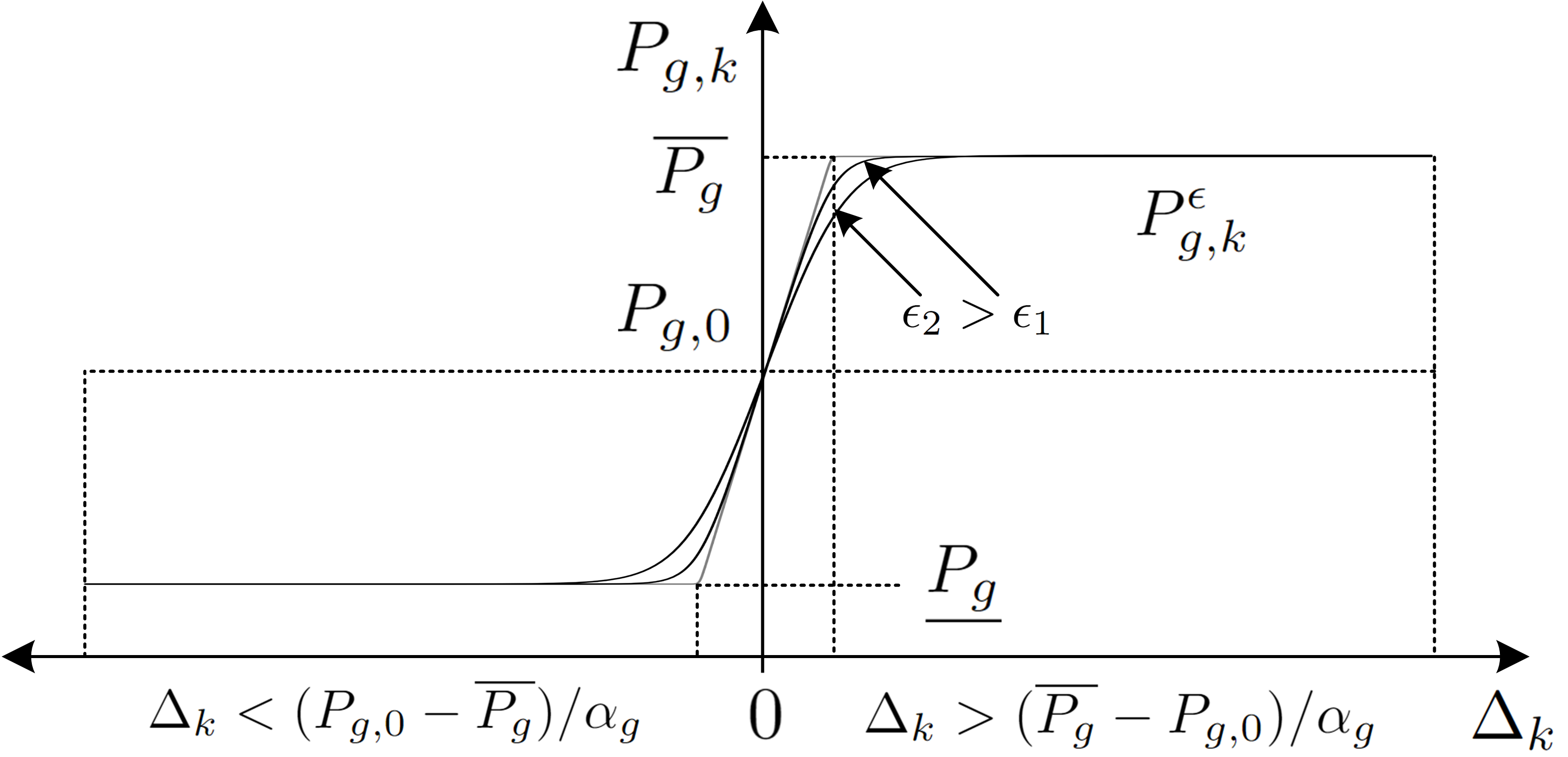
A generator responding in a contingency event adjusts its active power output by a common perturbation denoted by variable according to its predefined (offline) participation factor (droop slope) until it hits an operational bound , or as shown in Fig. 1. This is referred to as the generator’s post-contingency frequency response. The active power output of a responding generator in contingency is given as,
| (3) |
A generator that is online in a contingency but is not selected to respond to that contingency maintains its active power output from the base case,
| (4) |
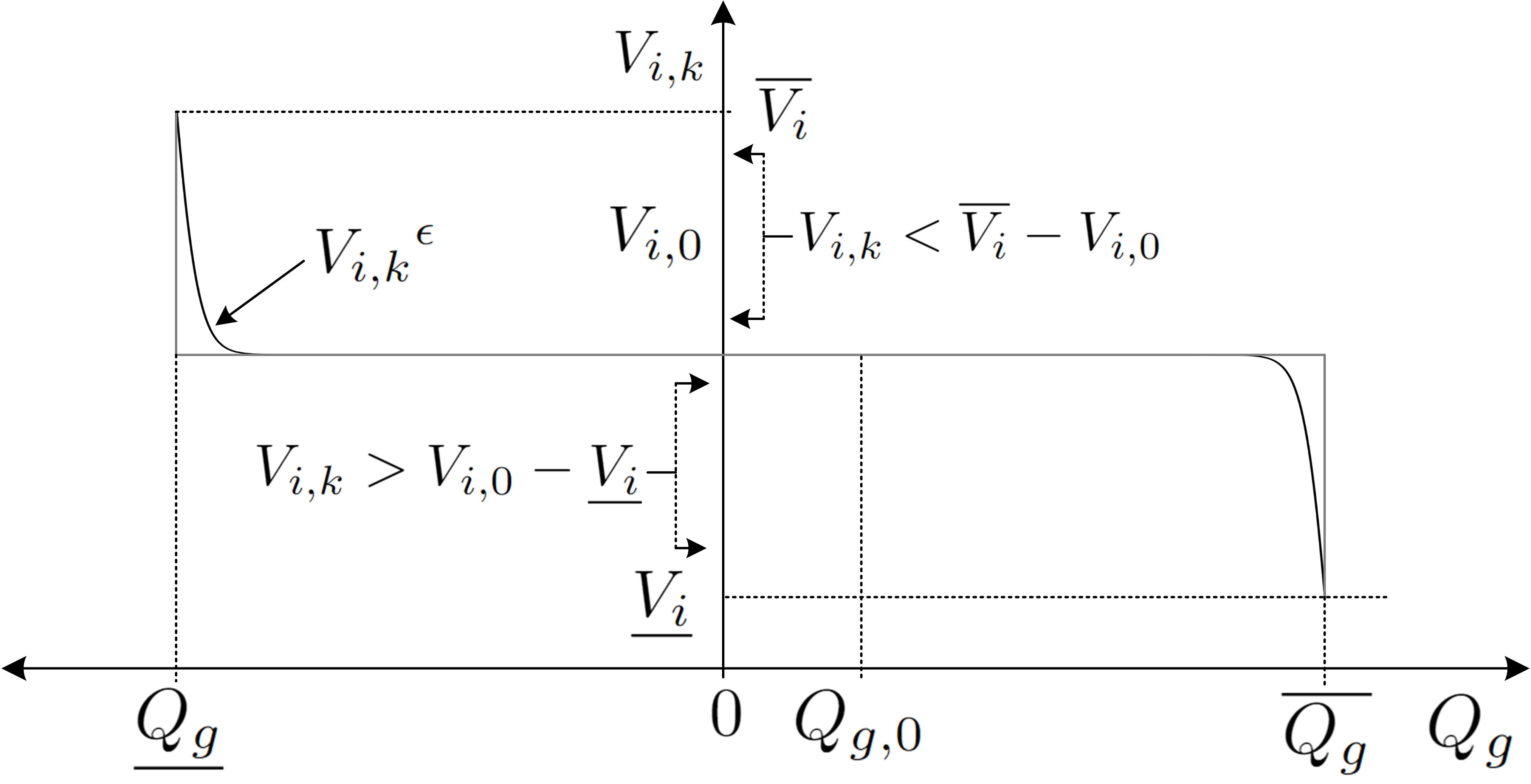
In a contingency event , a responding generator tries to maintain its voltage magnitude equal to the base case voltage by adjusting its reactive power unless it hits operational bounds or as shown in Fig. 2. This is referred to as PV/PQ bus switching control and modeled,
| (5) |
We convert conditional constraints (3) and (5) into continuously differentiable functions using smooth approximation (1). The constraint (3) can be written,
| (6) |
By applying (1), constraint (6) can be expressed,
| (7) |
The parameter can be used to regulate the degree of approximation accuracy as shown in Fig. 1, the approximation gap narrows for and further as . Similarly, with generator-node mapping , (5) can be stated,
| (8) |
where and represent the upper and lower margins of base case voltage from the bounds as,
| (9) | ||||
| (10) |
The necessary conditions for (8) are the voltage magnitude and generator reactive power bounds at these buses. By applying (1), the constraint (8) can be expressed as,
| (11) |
II-C HVDC Converter P–Vdc Droop Control Model
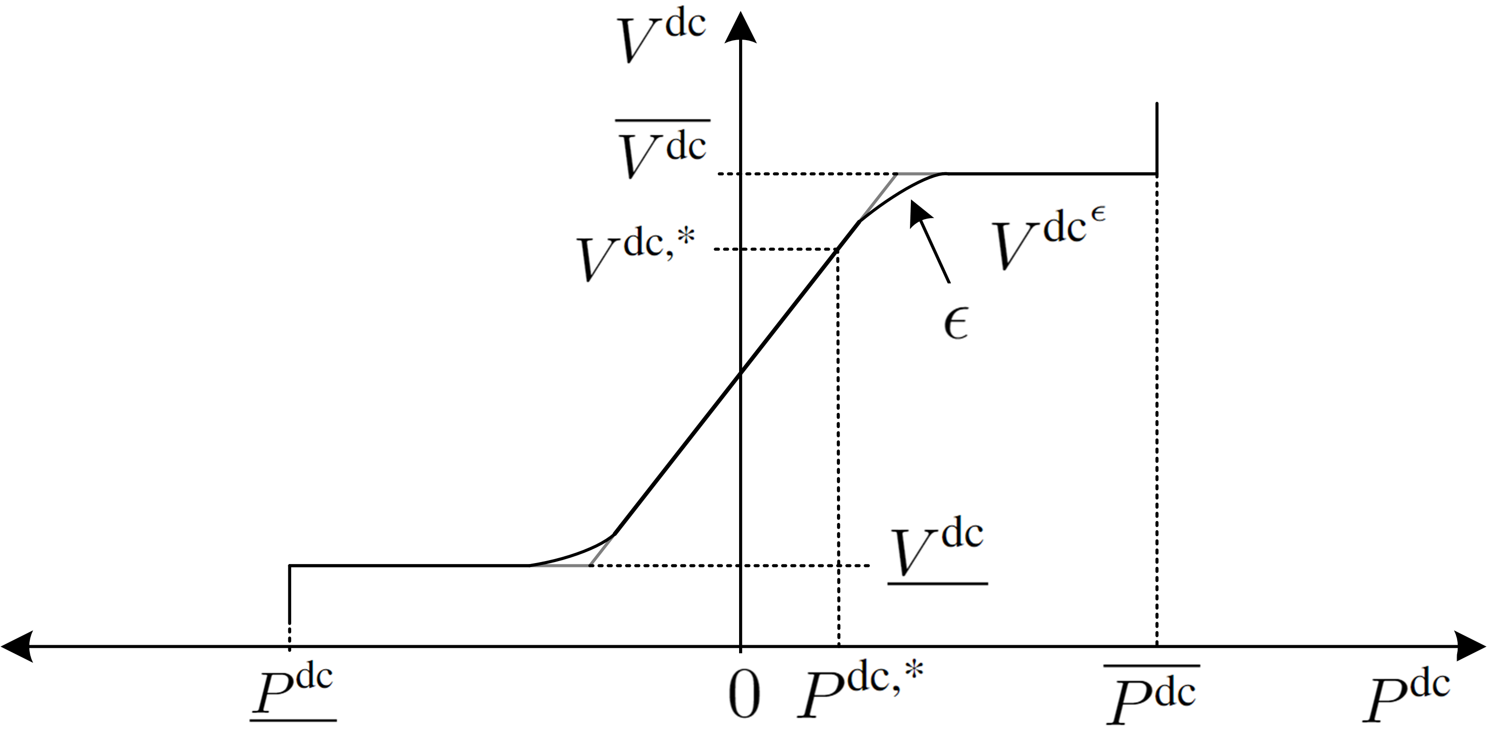
The P–Vdc linear droop control as shown in Fig. 3 is expressed by a relation between dc voltage at dc grid bus and the dc side power of converter , with the mapping and ,
| (12) |
where is the droop coefficient, denotes the reference dc side power, and is the reference dc voltage. The function returns the sign of the reference dc side power to represent both inverter and rectifier modes of operation.
The constraint (12) can be rewritten in the form of max functions explicitly for either of the sign conventions based on a given reference value,
| (13) |
Here, the converter dc power bounds are expressed as , and using (12).
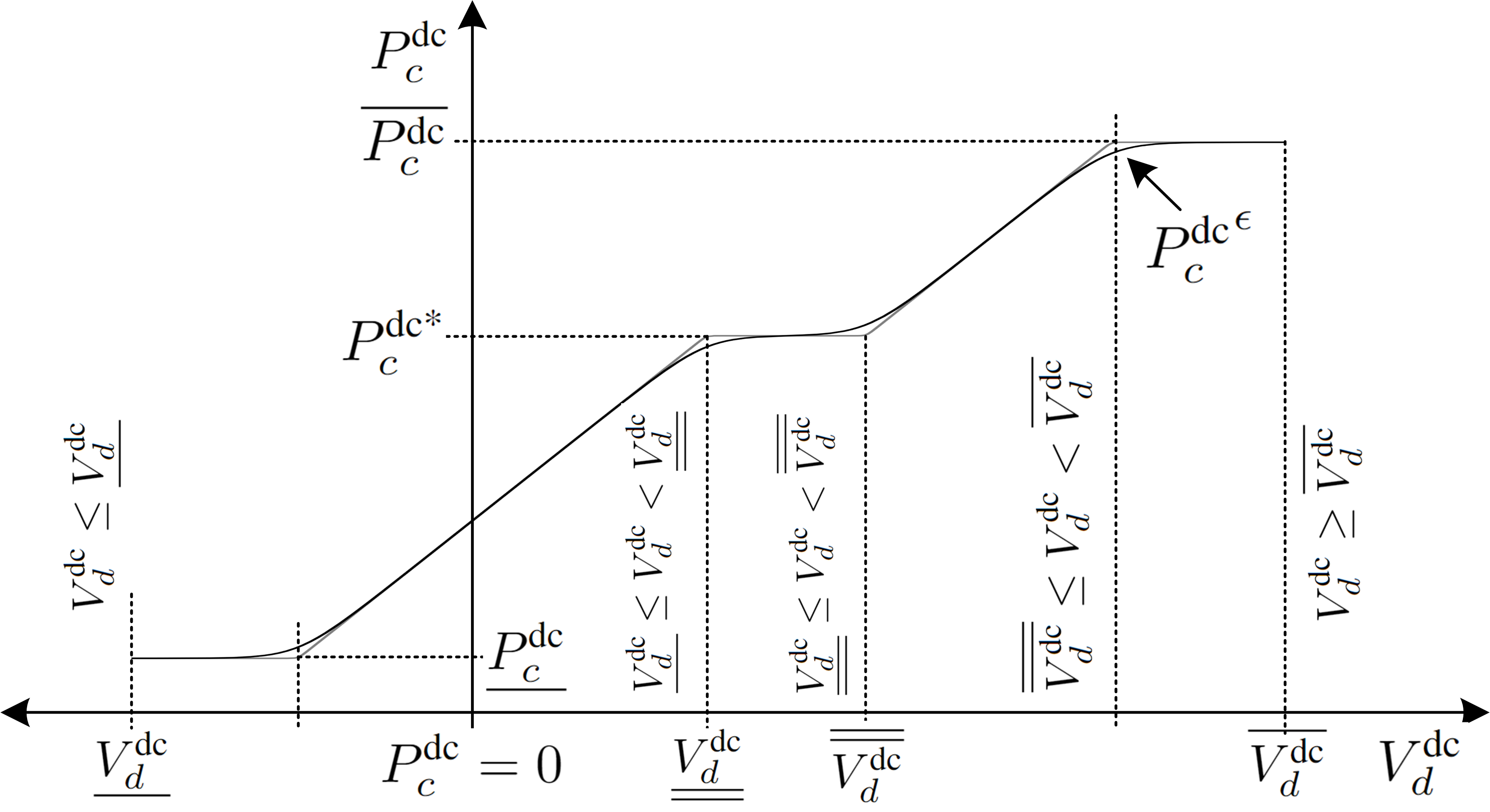
The P–Vdc piecewise linear droop control with power deadband and voltage limits as shown in Fig. 4 can be defined,
| (15) |
The converter operates in a constant power mode when the dc voltage is between and . When the voltage exceeds these limits, the droop control adjusts the power output of the converter until the voltage hits its bounds and . Similar to (12), a smooth function for (15) with voltage limits is,
| (16) |
When , can be implimented. For the PF application, (12) and (15) are implemented without limits and thus, this five-step piecewise linear droop function is extended beyond voltage bounds. Furthermore, power limits can also be imposed on (16) similar to (13) and (14). Finally, the same smooth functions can be adapted for Q–Vac droop control.
III Simulation Results
Two test datasets, case5 and case67 are used to perform PF, OPF, and, SCOPF simulations. The Ipopt and Juniper solvers are used for optimization models on a PC with Intel Core i9-11950H with 64 GB RAM. The test datasets, PF, OPF, and SCOPF models are publicly available as an open-source library PowerModelsACDCsecurityconstrained.jl’222https://github.com/csiro-energy-systems/PowerModelsACDCsecurityconstrained.jl.
III-A Comparing Proposed Models with/out Integer Variables
The section compares the proposed smooth approximation-based NLP models with the MINLP models for the PF, OPF and SCOPF problems considering steady-state voltage regulation in ac-dc power systems using P–Vdc and Q–Vac droop controls and generator PQ response functions. Five scenarios with the following response functions are studied:
-
i)
generator PQ droop;
-
ii)
generator PQ, and converter P-Vdc droops;
-
iii)
generator PQ, and converter P-Vdc w. deadband droops;
-
iv)
generator PQ, and converter P-Vdc, Q-Vac droops;
-
v)
generator PQ, and converter P-Vdc, Q-Vac w. deadband droops;
The numerical results, as presented in Table I, illustrate that the proposed smooth approximation-based NLP models significantly outperform the MINLP models in computational efficiency. While the objective function values remain largely consistent across the models, the incorporation of piecewise linear droop curves with deadbands in the MINLP models introduces additional binary variables (bvar), which increases the computation time. Notably, scenario v, characterized by the highest number of binary variables, exhibits the greatest computational burden. In the context of the SCOPF problem, the addition of each contingency substantially increases the number of continuous (cvar) and binary variables, rendering the problem increasingly challenging to solve. In the 67-bus case, in scenarios iii, iv, and v, MINLP SCOPF models could not be solved due to limited computational resources, whereas, the proposed NLP models efficiently solve these scenarios.
case sc. OPF MINLP Model OPF Propsoed NLP Model PF SCOPF MINLP Model SCOPF Propsoed NLP Model obj () time (s) bvar cvar obj () time (s) time (s) obj () time (s) bvar cvar obj () time (s) cvar 5 i 30 10.0 25 147 30 0.13 – 53.5276 244.4 88 1880 52.4455 13.644 1694 ii 30 16.4 45 147 30 0.10 0.11 53.6021 296.7 126 1880 53.6628 10.445 1694 iii 30 27.2 55 147 30 2.14 0.13 54.0348 288.4 153 1880 53.159 10.824 1694 iv 30 21.4 65 147 30 0.16 0.13 33853.1 520.2 198 1880 32470.9 9.961 1694 v 30 35.2 85 147 30 3.40 0.15 96558.4 578.5 218 1880 96487.7 18.732 1694 67 i 1.233e5 162.5 45 742 1.234e5 0.57 – 1.246e5 13178.4 512 6366 1.257e5 123.44 26756 ii 1.234e5 215.9 72 742 1.234e5 0.80 0.23 1.238e5 14376.3 768 9549 1.345e5 145.62 26756 iii 1.245e5 286.4 90 742 1.234e5 0.73 0.21 — — — — 1.246e6 106.33 21353 iv 1.247e5 1555.3 99 742 1.245e5 1.48 0.20 — — — — 1.340e5 126.81 29429 v 1.246e5 1836.1 135 742 1.245e5 1.14 0.22 — — — — 1.340e7 116.50 26756
III-B Voltage Regulation with P–Vdc and Q–Vac droop control
The proposed smooth approximation-based OPF models with and without P–Vdc only and P–Vdc, Q–Vac droop control are solved on case5 ac-dc power system with different load variations and the results are presented in Fig. 6. These results indicate that the implementation of P–Vdc and Q–Vac droop control substantially enhances voltage regulation. Furthermore, the findings underscore that the limited reactive power capacity of the HVDC converter necessitates allowing voltage drops only when the voltage reaches its bounds. This constraint highlights the importance of effectively managing reactive power within the system to maintain voltage stability under varying load conditions.
III-C Impact of Droop Coefficient and Deadband
This section evaluates the impact of different P–Vdc droop slopes and the implementation of droop control with and without deadband on voltage regulation under varying load conditions in the case5 ac-dc power system as shown in Fig. 7. The droop control without a deadband employs a fixed droop coefficient, balancing the trade-off between voltage regulation stiffness and power-sharing accuracy. A small droop coefficient such as 0.003 in comparison to 0.007 improves voltage regulation but sacrifice power-sharing and vice versa. Typically, system operators allow a maximum 10% DC voltage variation, allocating 5% for the line drops, thus limiting the voltage range available for droop control and consequently the droop coefficient. However, the droop control without a deadband cannot operate the converter in constant power control. In contrast, droop control with a deadband maintains the converters in constant power control when the voltage is between 0.98 and 1.02 pu, therefore providing better power-sharing under higher loads and better voltage regulation under light loads.
III-D Voltage Regulation with P–Vdc, Q–Vac Droop control and Generator PQ Response in Contingency Events
The proposed smooth approximation allows efficient implementation of the P–Vdc, Q–Vac droop control, and generator PQ response functions in the SCOPF problem. As illustrated in Fig. 8, the P–Vdc, Q–Vac droop control for case5 ac-dc power system efficiently regulates voltage and manages power-sharing during various contingency events such as generator, ac transmission line, transformer, converter, and dc transmission line contingencies. Specifically generator 3, as shown in Fig. 8, is an offshore wind farm connected to the mainland via a HVDC system with no reactive power capability. The P–Vdc droop control ensures the converters operate in constant power control mode by leveraging the sufficient active power response from generators during contingencies, thus maintaining the base-case voltage throughout the events and achieving the final solution. Meanwhile, the Q–Vac droop control considers converters’ limited reactive power capacity, effectively regulating ac bus voltages and adhering to reactive power and voltage constraints.
IV Conclusions
The proposed smooth approximation-based modeling enables implementation of generator PQ response, converters P–Vdc, Q–Vac droop control including voltage limits, power deadbands, and power limits in PF, OPF, and SCOPF applications. These models employ smooth (continuous and differentiable) functions that can be efficiently solved using Newton’s method or derivative-based interior point solvers. Numerical results demonstrate a substantial reduction in computational time compared to existing MINLP models. Furthermore, these models are fully parameterized and tuneable, offering flexibility for enhanced system efficiency, while the findings highlight improved voltage regulation and power-sharing during load variations and contingency events.
References
- Li et al. [2020] P. Li, C. Wang, Q. Wu, and M. Yang, “Risk-based distributionally robust real-time dispatch considering voltage security,” IEEE Trans. Sust. Energy, vol. 12, no. 1, pp. 36–45, 2020.
- He et al. [2023] X. He, V. Häberle, I. Subotić, and F. Dörfler, “Nonlinear stability of complex droop control in converter-based power systems,” IEEE Control Syst. Letters, vol. 7, pp. 1327–1332, 2023.
- Ismail et al. [2023] F. Ismail, J. Jamaludin, and N. Rahim, “Improved active and reactive power sharing on distributed generator using auto-correction droop control,” Electr. Power Syst.s Res., vol. 220, p. 109358, 2023.
- Chakraborty et al. [2023] S. Chakraborty, S. Patel, G. Saraswat, A. Maqsood, and M. V. Salapaka, “Seamless transition of critical infrastructures using droop controlled grid-forming inverters,” IEEE Trans. Indust. Electron., 2023.
- Hossen and Mirafzal [2022] T. Hossen and B. Mirafzal, “On stability of pq-controlled grid-following and droop-control grid-forming inverters,” in IEEE Energy Conv. Congress Expo. IEEE, 2022, pp. 1–7.
- Mohammed and Ciobotaru [2022] N. Mohammed and M. Ciobotaru, “Adaptive power control strategy for smart droop-based grid-connected inverters,” IEEE Trans. Smart Grid, vol. 13, no. 3, pp. 2075–2085, 2022.
- Singhal et al. [2022] A. Singhal, T. L. Vu, and W. Du, “Consensus control for coordinating grid-forming and grid-following inverters in microgrids,” IEEE Trans. Smart Grid, vol. 13, no. 5, pp. 4123–4133, 2022.
- Zhong and Konstantopoulos [2016] Q. Zhong and G. C. Konstantopoulos, “Current-limiting droop control of grid-connected inverters,” IEEE Trans. Ind. Elect., vol. 64, no. 7, pp. 5963–5973, 2016.
- Zhong and Zeng [2016] Q. Zhong and Y. Zeng, “Universal droop control of inverters with different types of output impedance,” IEEE access, vol. 4, pp. 702–712, 2016.
- Sun et al. [2023] P. Sun, Y. Wang, M. Khalid, R. Blasco-Gimenez, and G. Konstantinou, “Steady-state power distribution in vsc-based mtdc systems and dc grids under mixed p/v and i/v droop control,” Electr. Power Syst. Res., vol. 214, p. 108798, 2023.
- Lee et al. [2020] G.-S. Lee, D.-H. Kwon, S.-I. Moon, and P.-I. Hwang, “A coordinated control strategy for lcc hvdc systems for frequency support with suppression of ac voltage fluctuations,” IEEE Trans. Power Syst., vol. 35, no. 4, pp. 2804–2815, 2020.
- Ahrabi et al. [2020] R. R. Ahrabi, Y. W. Li, and F. Nejabatkhah, “Hybrid ac/dc network with parallel LCC-VSC interlinking converters,” IEEE Trans. Power Syst., vol. 36, no. 1, pp. 722–731, 2020.
- He et al. [2024] Y. He, W. Xiang, P. Meng, and J. Wen, “Investigation on grid-following and grid-forming control schemes of cascaded hybrid converter for wind power integrated with weak grids,” Int. J. Electr. Power Energy Syst., vol. 155, p. 109524, 2024.
- Li et al. [2021] D. Li, M. Sun, and Y. Fu, “A general steady-state voltage stability analysis for hybrid multi-infeed hvdc systems,” IEEE Trans. Power Del., vol. 36, no. 3, pp. 1302–1312, 2021.
- Ergun et al. [2024] H. Ergun, K. Yurtseven, G. Mohy-ud-din, and R. Heidari, “Robust and security-constrained optimisation of converter droop gains in meshed hvdc grids,” in IEEE Int. Conf. Probabilistic Methods Appl. Power Syst/, 2024, pp. 1–6.
- Chen et al. [2019] F. Chen, R. Burgos, D. Boroyevich, J. C. Vasquez, and J. M. Guerrero, “Investigation of nonlinear droop control in dc power distribution systems: Load sharing, voltage regulation, efficiency, and stability,” IEEE Trans. Power Elect., vol. 34, no. 10, pp. 9404–9421, 2019.
- Zhao et al. [2020] X. Zhao, H. Wei, J. Qi, P. Li, and X. Bai, “Frequency stability constrained optimal power flow incorporating differential algebraic equations of governor dynamics,” IEEE Trans. Power Syst., vol. 36, no. 3, pp. 1666–1676, 2020.
- Zhou et al. [2023] B. Zhou, R. Jiang, and S. Shen, “Frequency stability-constrained unit commitment: Tight approximation using bernstein polynomials,” IEEE Trans. Power Syst., 2023.
- Mohy-ud-din et al. [2023] G. Mohy-ud-din, R. Heidari, H. Ergun, and F. Geth, “An ac-dc power flow algorithm for Australian national electricity market,” in IEEE Int. Conf. Energy Tech. Future Grids, 2023, pp. 1–6.
- Ergun et al. [2019] H. Ergun, J. Dave, D. Van Hertem, and F. Geth, “Optimal power flow for ac-dc grids: Formulation, convex relaxation, linear approximation, and implementation,” IEEE Trans. Power Syst., vol. 34, no. 4, pp. 2980–2990, July 2019.
- Mohy-ud-din et al. [2024] G. Mohy-ud-din, R. Heidari, H. Ergun, and F. Geth, “Ac–dc security-constrained optimal power flow for the Australian national electricity market,” Electr. Power Syst. Res., vol. 234, p. 110784, 2024.
- Avella et al. [2023] P. Avella, A. Calamita, and L. Palagi, “A computational study of off-the-shelf minlp solvers on a benchmark set of congested capacitated facility location problems,” arXiv:2303.04216, 2023.
- Chen and Harker [1997] B. Chen and P. T. Harker, “Smooth approximations to nonlinear complementarity problems,” SIAM J. Optim., vol. 7, no. 2, pp. 403–420, 1997.