Absolute State-wise Constrained Policy Optimization: High-Probability State-wise Constraints Satisfaction

\nameWeiye Zhao \email[email protected] \AND\nameFeihan Li^∗ \email[email protected]\AND\nameYifan Sun \email[email protected] \AND\nameYujie Yang \email[email protected] \AND\nameRui Chen \email[email protected] \AND\nameTianhao Wei \email[email protected] \AND\nameChangliu Liu \email[email protected]
\addrRobotics Institute
Carnegie Mellon University
Pittsburgh, PA 15213, USA Equal Contribution

Abstract

Enforcing state-wise safety constraints is critical for the application of reinforcement learning (RL) in real-world problems, such as autonomous driving and robot manipulation. However, existing safe RL methods only enforce state-wise constraints in expectation or enforce hard state-wise constraints with strong assumptions. The former does not exclude the probability of safety violations, while the latter is impractical. Our insight is that although it is intractable to guarantee hard state-wise constraints in a model-free setting, we can enforce state-wise safety with high probability while excluding strong assumptions. To accomplish the goal, we propose Absolute State-wise Constrained Policy Optimization (ASCPO), a novel general-purpose policy search algorithm that guarantees high-probability state-wise constraint satisfaction for stochastic systems. We demonstrate the effectiveness of our approach by training neural network policies for extensive robot locomotion tasks, where the agent must adhere to various state-wise safety constraints. Our results show that ASCPO significantly outperforms existing methods in handling state-wise constraints across challenging continuous control tasks, highlighting its potential for real-world applications.

Keywords: State-wise Constraint, Constrained Policy Optimization, High-probability Constraints Satisfaction, Trust Region, Safe Reinforcement Learning

1 Introduction

In the reinforcement learning (RL) literature, safe RL is a specific branch that considers constraint satisfaction in addition to reward maximization (Achiam et al., 2017a). The explicit enforcement of constraint satisfaction is often critical to training RL agents for real-world deployments He et al. (2023a); Noren et al. (2021); Zhao et al. (2020b). That is because even if RL agents are penalized for violating safety constraints, they may still trade safety for overall higher rewards Zhao et al. (2019), which is unacceptable in many practical scenarios. For example, a self-driving car should never get too close to a pedestrian to save travel time. Safe RL aims to address such problems by treating the satisfaction of safety constraints separately from the maximization of task objectives Wei et al. (2024); Zhao et al. (2024c). To achieve that goal, it is important to properly model the safety constraints. Traditional RL builds on Markov Decision Processes (MDPs), which produce trajectories of agent states and actions as the result of agent-environment interactions. Under the framework, safety constraints can be defined in various forms. In general, constraints can be defined in a cumulative sense (Ray et al., 2019; Stooke et al., 2020; Achiam et al., 2017a; Yang et al., 2020) that the total safety violation from all states should be bounded. Constraints can also be defined state-wise, such that safety is ensured at each time step either in expectation (Pham et al., 2018; Amani and Yang, 2022; Zhao et al., 2024a) or almost surely under assumptions of system dynamics knowledge (Berkenkamp et al., 2017; Fisac et al., 2018; Wachi and Sui, 2020; Shi et al., 2023; Wachi et al., 2024a; Zhao et al., 2023c).

Refer to caption — Figure 1: Explanation of ASCPO principles. For simplicity, the distribution is assumed to be Gaussian. Green and blue represent the maximum and expectation of maximum state-wise cost distribution respectively. Y-axis represents the distribution of maximum state-wise cost samples (introduced in Section 3.1) across different initial states. ASCPO is designed to constrain the maximum state-wise cost under safety threshold ( $w_{i}$ ) while SCPO only focuses on constraining the expectation of state-wise cost and CPO (Achiam et al., 2017a) lacks the capability to ensure state-wise safety.

Ideally, safety constraints should be strictly satisfied at every time step He et al. (2023b); Zhao et al. (2023d). However, strictly satisfying safety constraints in a model-free setting is challenging, especially when the system has dynamic limits. Hence, in this paper, we consider a slightly relaxed yet still strong safety condition where constraints are guaranteed for each state with a configurable high probability (Wachi et al., 2024b). Notably, such a definition poses significantly stricter safety conditions than cumulative safety and is much more difficult to solve. The most recent advancement in that direction is state-wise constrained policy optimization (SCPO) (Zhao et al., 2024a), which enforces state-wise constraints. However, SCPO only considers constraint satisfaction in expectation without considering the variance of violations. As a result, safety constraints might still be violated at a non-trivial rate if the violations are long-tail distributed.

In this paper, we propose absolute state-wise constrained policy optimization (ASCPO) to guarantee state-wise safety constraints with a high probability. In addition to the expected constraint violation, which SCPO considers, ASCPO also considers the variance to constrain the probability upper bound of violations within a user-specified threshold. The main idea of ASCPO is illustrated in fig. 1. Through experiments, we demonstrate that ASCPO can achieve high rewards in high-dimensional tasks with state-of-the-art low safety violations. Our code is available on Github.¹¹1https://github.com/intelligent-control-lab/Absolute-State-wise-Constrained-Policy-Optimization Our contribution is summarized below:

•

To the best of the authors’ knowledge, the proposed approach is the first policy optimization method to ensure high-probability satisfaction of state-wise safety constraints without assuming knowledge of the underlying dynamics.

2 Related Work

In safe reinforcement learning (RL), there are two main types of safety specifications: cumulative safety and state-wise safety. Here we primarily discuss state-wise safe RL methods. Interested readers can refer to survey papers (Liu et al., 2021; Gu et al., 2022; Brunke et al., 2022; Wachi et al., 2024b) for more comprehensive discussions. Specifically, state-wise safety (instantaneous safety) aims to constrain the instantaneous cost at every step. In a stochastic environment, strictly satisfying a state-wise safety constraint at every step is impractical because the instantaneous cost is a random variable under a possibly unbounded distribution. Therefore, existing methods either constrain the instantaneous cost at each step in expectation or ensure a high probability of satisfying instantaneous constraints at all steps.

Constraint in expectation

To enforce expected state-wise constraints, OptLayer (Pham et al., 2018) uses a safety layer that modifies potentially unsafe actions generated by a reward-maximizing policy to constraint-satisfying ones. Zhao et al. introduce state-wise constrained policy optimization (SCPO) that guarantees to constrain the maximum violation along a trajectory in expectation based on a novel Maximum MDP framework. Similar idea of constraining the maximum violation can also be found in Hamilton-Jacobi (HJ) reachability analysis (Bansal et al.), which computes a value function to represent the maximum violation in the future. The HJ reachability value function is widely used to learn safety-oriented policies or build constraints for policy optimization in safe RL (Fisac et al.; Yu et al.). Although these methods take state-wise safety into consideration, their constraint in expectation formulations still fall short of controlling the distributions of instantaneous safety violations.

High-probability Constraint

Existing safe exploration literature primarily focuses on addressing high-probability and even surely state-wise constraint satisfaction (Zhao et al., 2023a), including (i) structural solutions and (ii) end-to-end solutions. Structural solutions construct a hierarchical safe agent with an upper layer generating reference actions and a lower layer performing safe action projection at every time step. To achieve this, prior knowledge about system dynamics is required Wei et al. (2022); Zhao et al. (2020a, 2022); Chen et al. (2024a, b); Li et al. (2023), such as analytical dynamics (Cheng et al., 2019; Shao et al., 2021; Fisac et al., 2018; Ferlez et al., 2020), black-box dynamics (Zhao et al., 2021, 2024b), learned dynamics (Dalal et al., 2018; Zhang et al., 2022b; Bharadhwaj et al., 2020; Chow et al., 2019; Thananjeyan et al., 2021), or the Lipschitzness bound of dynamics (Zhao et al., 2023b). Similarly, end-to-end solutions ensure safe actions by considering the uncertainty of learned dynamics at every time step, where high-probability state-wise safety guarantees stem from the knowledge of the Lipschitzness bound of dynamics (Berkenkamp et al., 2017; Wachi et al., 2018, 2024a) and constraints (Wachi and Sui, 2020) or evaluable black-box system dynamics (Wachi and Sui, 2020).

In contrast, our method directly ensures high-probability state-wise constraint satisfaction without assumptions on knowledge of the underlying dynamics.

3 Problem Formulation

3.1 State-wise Constrained Markov Decision Process

This paper studies the persistent satisfaction of cost constraints at every step for episodic tasks, in the framework of State-wise Constrained Markov Decision Process (SCMDP) (Zhao et al., 2023a) for finite horizon. An finite horizon MDP finishes within $H\in\mathbb{N}$ steps, and is specified by a tuple $(\mathcal{S},\mathcal{A},\gamma,R,P,\mu)$ , where $\mathcal{S}$ is the state space, and $\mathcal{A}$ is the control space, $R:\mathcal{S}\times\mathcal{A}\mapsto\mathbb{R}$ is the reward function, $0\leq\gamma<1$ is the discount factor, $\mu:\mathcal{S}\mapsto\mathbb{R}$ is the initial state distribution, and $P:\mathcal{S}\times\mathcal{A}\times\mathcal{S}\mapsto\mathbb{R}$ is the transition probability function. $P(s^{\prime}|s,a)$ is the probability of transitioning to state $s^{\prime}$ given that the previous state was $s$ and the agent took action $a$ at state $s$ . Building upon MDP, SCMDP introduces a set of cost functions, $C_{1},C_{2},\cdots,C_{m}$ , where $C_{i}:\mathcal{S}\times\mathcal{A}\times\mathcal{S}\rightarrow\mathbb{R}$ maps the state action transition tuple into a cost value. A stationary policy $\pi:\mathcal{S}\mapsto\mathcal{P}(\mathcal{A})$ is a map from states to a probability distribution over actions, with $\pi(a|s)$ denoting the probability of selecting action $a$ in state $s$ . We denote the set of all stationary policies by $\Pi$ .

The goal for SCMDP is to learn a policy $\pi$ that maximizes a performance measure $\mathcal{J}_{0}(\pi)\doteq\mathbb{E}_{\tau\sim\pi}\left[\sum_{t=0}^{H}\gamma^{t}R(s_{t},a_{t},s_{t+1})\right]$ , so that the cost for every state action transition satisfies a constraint. Formally,

\displaystyle\underset{\pi}{\textbf{max}}\leavevmode\nobreak\ \mathcal{J}_{0}(\pi),\leavevmode\nobreak\ \textbf{s.t.}\leavevmode\nobreak\ \forall i,\forall(s_{t},a_{t},s_{t+1})\sim\tau,C_{i}(s_{t},a_{t},s_{t+1})\leq w_{i}

(1)

where $\tau=[s_{0},a_{0},s_{1},\cdots]$ and $\tau\sim\pi$ , $w_{i}\in\mathbb{R}$ . Here $\tau\sim\pi$ is shorthand for that the distribution over trajectories depends on $\pi:s_{0}\sim\mu,a_{t}\sim\pi(\cdot|s_{t}),s_{t+1}\sim P(\cdot|s_{t},a_{t})$ .

Restricting Maximum Cost

It is noteworthy that for (1), each state-action transition pair introduces a constraint, leading to a computational complexity that increases nearly cubically as the MDP horizon ( $H$ ) grows (Zhao et al., 2024a). Instead of directly constraining the cost of each possible state-action transition, it is easier to constrain the maximum state-wise cost along the trajectory. To efficiently compute the maximum state-wise cost, we follow maximum Markov decision process (MMDP) (Zhao et al., 2024a) to introduce (i) a set of up-to-now maximum state-wise costs $\textbf{M}\doteq[M_{1},M_{2},\cdots,M_{m}]$ where $M_{i}\in\mathcal{M}_{i}\subset\mathbb{R}$ , and (ii) a set of cost increment functions, $D_{1},D_{2},\cdots,D_{m}$ , where $D_{i}:(\mathcal{S},\mathcal{M}_{i})\times\mathcal{A}\times\mathcal{S}\mapsto[0,\mathbb{R}^{+}]$ maps the augmented state action transition tuple into a nonnegative cost increment. We define the augmented state ${\hat{s}}=(s,\textbf{M})\in(\mathcal{S},\mathcal{M}^{m})\doteq\hat{\mathcal{S}}$ , where $\hat{\mathcal{S}}$ is the augmented state space with $\mathcal{M}^{m}=(\mathcal{M}_{1},\mathcal{M}_{2},\cdots,\mathcal{M}_{m})$ . Formally,

\displaystyle D_{i}\big{(}{\hat{s}}_{t},a_{t},{\hat{s}}_{t+1}\big{)}=\max\{C_{i}(s_{t},a_{t},s_{t+1})-{M_{it}},0\},i\in 1,\cdots,m.

(2)

Setting $D_{i}\big{(}{\hat{s}}_{0},a_{0},{\hat{s}}_{1}\big{)}=C_{i}(s_{0},a_{0},s_{1})$ , we have $M_{it}=\sum_{k=0}^{t-1}D_{i}\big{(}{\hat{s}}_{k},a_{k},{\hat{s}}_{k+1}\big{)}$ for $t\geq 1$ . Hence, we define the maximum state-wise cost performance sample for $\pi$ as:

\displaystyle{\mathcal{D}_{i}}_{\pi}(\hat{s}_{0})=\sum_{t=0}^{H}D_{i}\big{(}{\hat{s}}_{t},a_{t},{\hat{s}}_{t+1}\big{)},

(3)

where the state action sequence $\hat{\tau}=[a_{0},{\hat{s}}_{1},\dots]\sim\pi$ starts with an initial state $\hat{s}_{0}$ , which follows initial state distribution $\mu$ . The intuition of MMDP is illustrated in Figure 2. With (3), (1) can be rewritten as:

\displaystyle\underset{\pi}{\textbf{max}}\leavevmode\nobreak\ \mathcal{J}(\pi),\leavevmode\nobreak\ \textbf{s.t.}\leavevmode\nobreak\ \forall i,\leavevmode\nobreak\ {\mathcal{D}_{i}}_{\pi}(\hat{s}_{0})\leq w_{i},

(4)

where $\mathcal{J}(\pi)=\mathbb{E}_{\tau\sim\pi}\left[\sum_{t=0}^{H}\gamma^{t}R({\hat{s}}_{t},a_{t},{\hat{s}}_{t+1})\right]$ and $R({\hat{s}},a,{\hat{s}}^{\prime})\doteq R(s,a,s^{\prime})$ .

Remark 1

We would like to highlight the core differences between (4) and Constrained Markov Decision Processes (CMDP). Although (4) may appear similar to CMDP due to the inclusion of cost increments, the nature of the constraints is fundamentally different. Specifically, the constraints in (4) take the form of a non-discounted summation over a finite horizon, whereas CMDP considers a discounted summation over an infinite horizon. Additionally, (4) restricts the constraint satisfaction for each individual performance sample, whereas CMDP only requires constraint satisfaction for expected performance. Consequently, conventional techniques or theories used to solve CMDP are not applicable here.

With $R(\tau)$ being the discounted return of a trajectory with infinite horizon, we define the on-policy value function as $V_{\pi}({\hat{s}})\doteq\mathbb{E}_{\tau\sim\pi}[R(\tau)|{\hat{s}}_{0}={\hat{s}}]$ , the on-policy action-value function as $Q_{\pi}({\hat{s}},a)\doteq\mathbb{E}_{\tau\sim\pi}[R(\tau)|{\hat{s}}_{0}={\hat{s}},a_{0}=a]$ , and the advantage function as $A_{\pi}({\hat{s}},a)\doteq Q_{\pi}({\hat{s}},a)-V_{\pi}({\hat{s}})$ . Lastly, we define on-policy value functions, action-value functions, and advantage functions for the cost increments in analogy to $V_{\pi}$ , $Q_{\pi}$ , and $A_{\pi}$ . Similarly, we can define $V^{H}_{\pi}$ , $Q^{H}_{\pi}$ , and $A^{H}_{\pi}$ for trajectory with $H$ horizon. With $D_{i}$ replacing $R$ , respectively. We denote those by $V^{H}_{[D_{i}]\pi}$ , $Q^{H}_{[D_{i}]\pi}$ and $A^{H}_{[D_{i}]\pi}$ .

The idea of restricting the maximum cost in a trajectory is widely used in safe RL to ensure state-wise constraint satisfaction (Fisac et al., 2019; Yu et al., 2022). In addition to MMDP formulation, another method to achieve this goal is HJ reachability analysis (Bansal et al., 2017), which computes a value function to represent the maximum cost along the trajectory starting from the current state:

F_{i\pi}(s_{0})=\max_{t=0,1,\dots,H}C_{i}(s_{t},a_{t},s_{t+1}),

(5)

where $F_{i\pi}$ is the HJ reachability value function of the $i$ -th cost under policy $\pi$ . Compared with MMDP, HJ reachability analysis directly computes the maximum cost using the maximum operator, while MMDP transforms the maximum computation into a summation by introducing cost increment functions. Mathematically, $F_{i\pi}$ in HJ reachability analysis equals $\mathcal{D}_{i\pi}$ in MMDP at the initial state of a trajectory. Therefore, we can equivalently replace $\mathcal{D}_{i\pi}(\hat{s}_{0})$ with $F_{i\pi}(s_{0})$ in the constraint of problem (4). However, the advantage of using MMDP formulation is that the summation operator in $\mathcal{D}_{i\pi}$ enables us to use existing theoretical tools to derive bounds on the maximum state-wise cost, which is crucial for constraint satisfaction guarantee (Zhao et al., 2024a). In contrast, deriving similar cost bounds for Hamilton-Jacobi (HJ) reachability analysis is challenging due to the maximum operator in $F_{i\pi}$ . So far, this max and the associated error bounds can only be evaluated using traditional HJ methods, and no learning-based HJ method is capable of simultaneously evaluating the max and the associated error bounds. To the best of our knowledge, no existing HJ-reachability-based safe RL methods have established such bounds.

3.2 Upper Probability Bound of Maximum State-wise Cost

Restricting every possible maximum state-wise cost performance sample in (4) is impractical since ${\mathcal{D}_{i}}_{\pi}(\hat{s}_{0})$ is a continuous random variable under a possibly unbounded distribution. The best we can do is to restrict the upper probability bound (Pishro-Nik, 2014) of the maximum state-wise cost performance with high confidence, defined as:

Definition 1 (Upper Probability Bound of Constraint Satisfaction)

Given a tuple $(\mathcal{B}\in\mathbb{R},p\in\mathbb{R}^{+})$ , $\mathcal{B}$ is defined as the upper probability bound with confidence ${p}$ . Mathematically:

\displaystyle Pr\big{(}\mathcal{D}_{i\pi}(\hat{s}_{0})\leq\mathcal{B}\big{)}\geq p\leavevmode\nobreak\ .

(6)

Proposition 1

For an unknown distribution of random variable $\mathcal{D}_{i\pi}(\hat{s}_{0})$ , denote
$\mathcal{E}_{[D_{i}]}(\pi),\mathcal{V}_{[D_{i}]}(\pi)$ as the expectation and variance of the distribution, i.e.
$\mathcal{E}_{[D_{i}]}(\pi)=\mathbb{E}_{\hat{s}_{0}\sim\mu,\hat{\tau}\sim\pi}[\mathcal{D}_{i\pi}(\hat{s}_{0})]$ , $\mathcal{V}_{[D_{i}]}(\pi)=\mathbb{V}ar_{\hat{s}_{0}\sim\mu,\hat{\tau}\sim\pi}[\mathcal{D}_{i\pi}(\hat{s}_{0})]$ . $\mathcal{B}_{[D_{i}]k}(\pi)\doteq\mathcal{E}_{[D_{i}]}(\pi)+k\mathcal{V}_{[D_{i}]}(\pi)$ is guaranteed to be a upper probability bound of $\mathcal{D}_{i\pi}(\hat{s}_{0})$ in 1 with confidence $p_{k}^{\psi}\doteq 1-\frac{1}{k^{2}\psi+1}\in(0,1)$ . Here $k$ is the probability factor ( $k\geq 0$ , $k\in\mathbb{R}$ ) and $\psi=\mathcal{V}_{min}\in\mathbb{R}^{+}$ , where $\mathcal{V}_{min}$ is the minima of $\mathcal{V}_{[D_{i}]}(\pi)$ .

Remark 2

1 is proved in Section A.1. 1 shows that more than $p_{k}^{\psi}$ of the samples from the distribution of $\mathcal{D}_{i\pi}(\hat{s}_{0})$ will be smaller than the bound $\mathcal{B}_{[D_{i}]k}(\pi)$ . Given a positive constant $\psi$ , we can make $p_{k}^{\psi}\rightarrow 1$ by setting a large enough $k$ , so that $\mathcal{B}_{[D_{i}]k}(\pi)$ represents the upper probability bound of $\mathcal{D}_{i\pi}(\hat{s}_{0})$ with with a confidence level close to 1.

3.3 Policy Optimization Problem

In this paper, we focus on restricting the upper probability bound of maximum state-wise cost performance in SCMDP. In accordance with 1, the overarching objective is to identify a policy $\pi$ that effectively maximizes the performance measure and ensures $\mathcal{B}_{k}(\pi)<w$ . Mathematically,

\displaystyle\underset{\pi}{\leavevmode\nobreak\ \textbf{max}}\leavevmode\nobreak\ \mathcal{J}(\pi),\leavevmode\nobreak\ \textbf{s.t.}\leavevmode\nobreak\ \forall i,\leavevmode\nobreak\ {\mathcal{E}}_{[D_{i}]}(\pi)+k{\mathcal{V}}_{[D_{i}]}(\pi)\leq w_{i}.

(7)

4 Absolute State-wise Constrained Policy Optimization

Table 1: Notation Table of ASCPO I

Notation	Description
$\mathcal{S}$	State space
$\mathcal{A}$	Action space
$\mathcal{M}$	Up-to-now maximum state-wise cost space: $\mathcal{M}\subset\mathbb{R}$
$\hat{\mathcal{S}}$	Augmented state space
$\gamma$	Discount factor: $0\leq\gamma<1$
$R$	Reward function: $\mathcal{S}\times\mathcal{A}\mapsto\mathbb{R}$
$P$	Transition probability function: $\mathcal{S}\times\mathcal{A}\times\mathcal{S}\mapsto\mathbb{R}$
$\mu$	Initial state distribution: $\mathcal{S}\mapsto\mathbb{R}$
$C$	Cost function: $\mathcal{S}\times\mathcal{A}\times\mathcal{S}\rightarrow\mathbb{R}$
$D$	Cost increment function: $(\mathcal{S},\mathcal{M})\times\mathcal{A}\times\mathcal{S}\mapsto[0,\mathbb{R}^{+}]$
$\mathcal{P}(\mathcal{A})$	Probability distribution over actions
$\pi$	Stationary policy: $\mathcal{S}\mapsto\mathcal{P}(\mathcal{A})$
$\Pi$	Set of all stationary policies
$t$	Time step along the trajectory
$m$	Number of the constraints
$i$	Index of the constraints
$k$	Index of the policy update iterations
$w$	Maximum cost for constraints
$s_{t}$	State at step $t$ : $s\in\mathcal{S}$
$a_{t}$	Action at step $t$ : $a\in\mathcal{A}$
$M_{t}$	Up-to-now maximum state-wise cost at step $t$ : $M\in\mathcal{M}$
$\hat{s}_{t}$	Augmented state at step $t$ : $\hat{s}\in\hat{\mathcal{S}}$
$\tau$	Trajectory: a sequence of action and state
$H/h$	Horizon of a trajectory
$\pi(a\|s)$	Probability of selecting action $a$ in state $s$
$\pi(\cdot\|s)$	Probability distribution of all action in state $s$
$P(\cdot\|s,a)$	Probability distribution of all next state in state $s$ with action $a$
$\mathcal{J}(\pi)$	Expectation performance of policy $\pi$
$\mathcal{D}_{\pi}(\hat{s}_{0})$	Maximum state-wise cost performance sample of policy $\pi$
$R(\tau)$	Discounted return of a trajectory with infinite horizon
$V_{\pi}$	Value function with infinite horizon of policy $\pi$
$Q_{\pi}$	Action-value function with infinite horizon of policy $\pi$
$A_{\pi}$	Advantage function with infinite horizon of policy $\pi$
$V^{H}_{\pi}$	Value function with $H$ horizon of policy $\pi$
$Q^{H}_{\pi}$	Action-value function with $H$ horizon of policy $\pi$
$A^{H}_{\pi}$	Advantage function with $H$ horizon of policy $\pi$

Table 2: Notation Table of ASCPO II

$V^{H}_{[D]\pi}$	Value function of cost increment $D$ with $H$ horizon of policy $\pi$
$Q^{H}_{[D]\pi}$	Action-value function of cost increment $D$ with $H$ horizon of policy $\pi$
$A^{H}_{[D]\pi}$	Advantage function of cost increment $D$ with $H$ horizon of policy $\pi$
$F_{\pi}$	HJ reachability value functio
$\mathcal{B}$	Upper probability bound
${p}$	Confidence of the probability bound
$k$	Probability factor: $k\geq 0$ , $k\in\mathbb{R}$
$\mathcal{V}_{min}$	The minima of $\mathcal{D}_{\pi}(\hat{s}_{0})$
$\psi$	$\mathcal{V}_{min}\in\mathbb{R}^{+}$
$\mathcal{E}_{[D]}(\pi)$	Expectation of the distribution of $\mathcal{D}_{\pi}(\hat{s}_{0})$
$\mathcal{V}_{[D]}(\pi)$	Variance of the distribution of $\mathcal{D}_{\pi}(\hat{s}_{0})$
$\mathcal{B}_{[D]k}(\pi)$	Upper probability bound of $\mathcal{D}_{\pi}(\hat{s}_{0})$ with confidence $p_{k}^{\psi}$
$\mathcal{J}^{l}_{\pi,\pi_{j}}$	Surrogate function for policy update to bound $\mathcal{J}(\pi)$ from below
$\mathcal{E}^{u}_{[D]\pi,\pi_{j}}$	Surrogate function for policy update to bound $\mathcal{E}_{[D]}(\pi)$ from above
$\overline{MV}_{[D]\pi,\pi_{j}}$	Upper bound of expected variance of the maximum state-wise cost
$\overline{VM}_{[D]\pi,\pi_{j}}$	Upper bound of the variance of the expected maximum state-wise cost
$\mathcal{D}_{KL}(\pi\\|\pi_{j})[{\hat{s}}]$	KL divergence between two policies $(\pi,\pi_{j})$ at state $\hat{s}$
$d_{\pi}$	Discounted future state distribution of policy $\pi$
$\bar{d}_{\pi}$	Non-discounted future state distribution of policy $\pi$
$\epsilon_{[D]}^{\pi}$	Maximum expected advantage of policy $\pi$
${\mathcal{R}}_{\pi}(\hat{s}_{0})$	Discounted return starts at state $s_{0}$ with infinite horizon of policy $\pi$
$V_{\pi}(\hat{s}_{0})$	Value of state $\hat{s}_{0}$ with infinite horizon of policy $\pi$
${\mathcal{R}}_{\pi}^{H}\hat{s}_{0})$	Discounted return starts at state $s_{0}$ with $H$ horizon of policy $\pi$
$V_{\pi}^{H}(\hat{s}_{0})$	Value of state $\hat{s}_{0}$ with $H$ horizon of policy $\pi$
$\mathcal{E}(\pi)$	Expectation of the distribution of ${\mathcal{R}}_{\pi}(\hat{s}_{0})$ of policy $\pi$
$\mathcal{V}(\pi)$	Variance of the distribution of ${\mathcal{R}}_{\pi}(\hat{s}_{0})$ of policy $\pi$
$\mathcal{B}_{k}(\pi,\gamma)$	Upper probability bound of ${\mathcal{R}}_{\pi}(\hat{s}_{0})$
$MV_{\pi}$	MeanVariance of policy ${\pi}$
$VM_{\pi}$	VarianceMean of policy ${\pi}$
$\omega_{\pi}^{h}(\hat{s})$	Variance of the state-action value function ${Q^{h}_{\pi}}$ at state ${\hat{s}}$ with $h$ horizon
$\omega_{[D]\pi}^{h}(\hat{s})$	Variance of the state-action value function $Q^{h}_{[D]\pi}$ at state ${\hat{s}}$ with $h$ horizon
$\bm{\Omega}_{\pi}^{h}$	The vector of $\omega_{\pi}^{h}(\hat{s})$
$\bm{\Omega}_{[D]\pi}^{h}$	The vector of $\omega_{[D]\pi}^{h}(\hat{s})$
$\xi$	Action probability ratio

To optimize (7), we need to evaluate the objective and constraints under an unknown $\pi$ . While the exact computations of $\mathcal{J}(\pi)$ , ${\mathcal{E}}_{[D_{i}]}(\pi)$ , and ${\mathcal{V}}_{[D_{i}]}(\pi)$ are infeasible before the actual rollout, we can alternatively find surrogate functions for the objective and constraints of (7) such that (i) they provide a tight lower bound for the objective and a tight upper bound for the constraints, and (ii) they can be easily estimated from samples collected from the most recent policy.

Therefore, we introduce (i) $\mathcal{J}^{l}_{\pi,\pi_{j}}$ as a surrogate function to bound $\mathcal{J}(\pi)$ from below, (ii) $\leavevmode\nobreak\ \leavevmode\nobreak\ \mathcal{E}^{u}_{[D_{i}]\pi,\pi_{j}}$ as a surrogate function to bound $\mathcal{E}_{[D_{i}]}(\pi)$ from above, and (iii)
$\left(\overline{MV}_{[D_{i}]\pi,\pi_{j}}+\overline{VM}_{[D_{i}]\pi,\pi_{j}}\right)$ as a surrogate function to bound $\mathcal{V}_{[D_{i}]}(\pi)$ from above, in the $(j+1)$ -th iteration. All three surrogate functions could be estimated using samples from $\pi$ . Notice that the upper bound of $\mathcal{V}_{[D_{i}]}(\pi)$ involves two terms, where $\overline{MV}_{[D_{i}]\pi,\pi_{j}}$ reflects the upper bound of expected variance of the maximum state-wise cost over different start states. $\overline{VM}_{[D_{i}]\pi,\pi_{j}}$ reflects the upper bound of variance of the expected maximum state-wise cost of different start states. The detailed interpretations are shown in fig. 3.

4.1 Surrogate Functions for Objective and Constraints

In the following discussion, we derive the surrogate functions $\mathcal{J}^{l}_{\pi,\pi_{j}}$ , $\leavevmode\nobreak\ \leavevmode\nobreak\ \mathcal{E}^{u}_{[D_{i}]\pi,\pi_{j}}$ , $\overline{MV}_{[D_{i}]\pi,\pi_{j}}$ , and $\overline{VM}_{[D_{i}]\pi,\pi_{j}}$ .

Lower Bound for Objective

To bound the objective below, we directly follow the policy performance bound introduced by Achiam et al., which provides a tight lower bound for the objective. Mathematically,

\displaystyle\mathcal{J}^{l}_{\pi,\pi_{j}}\doteq\mathcal{J}(\pi_{j})+\frac{1}{1-\gamma}\underset{\begin{subarray}{c}\begin{subarray}{c}\hat{s}\sim d^{\pi_{j}}\\ a\sim{\pi}\end{subarray}\end{subarray}}{\mathbb{E}}\bigg{[}A^{H}_{\pi_{j}}(\hat{s},a)-\frac{2\gamma\epsilon^{\pi}}{1-\gamma}\sqrt{\frac{1}{2}\mathcal{D}_{KL}({\pi}\|\pi_{j})[\hat{s}]}\bigg{]}.

(8)

where $\mathcal{D}_{KL}(\pi\|\pi_{j})[{\hat{s}}]$ is the KL divergence between two policies $(\pi,\pi_{j})$ at state $\hat{s}$ and $d_{\pi_{j}}\doteq(1-\gamma)\sum\limits_{t=0}^{H}\gamma^{t}P({\hat{s}}_{t}={\hat{s}}|{\pi_{j}})$ is the discounted future state distribution.

Upper Bound of Maximum State-wise Cost Expectation

Different from $\mathcal{J}(\pi)$ , ${\mathcal{E}}_{[D_{i}]}(\pi)$ takes the form of a non-discounted summation over a finite horizon. Here we follow the tight upper bound of ${\mathcal{E}}_{[D_{i}]}(\pi)$ introduced by SCPO from Zhao et al.,

\displaystyle\mathcal{E}^{u}_{[D_{i}]\pi,\pi_{j}}\doteq\mathcal{E}_{[D_{i}]}(\pi)+\underset{\begin{subarray}{c}{\hat{s}}\sim\bar{d}_{\pi_{j}}\\ a\sim\pi\end{subarray}}{\mathbb{E}}\Bigg{[}A_{[D_{i}]\pi_{j}}^{H}({\hat{s}},a)+2(H+1)\epsilon_{[D_{i}]}^{\pi}\sqrt{\frac{1}{2}\mathbb{E}_{{\hat{s}}\sim\bar{d}_{\pi_{j}}}[\mathcal{D}_{KL}(\pi\|\pi_{j})[{\hat{s}}]]}\Bigg{]}.

(9)

where $\epsilon_{[D_{i}]}^{\pi}\doteq\underset{\hat{s}}{\mathbf{max}}|\underset{a\sim\pi}{\mathbb{E}}[A^{H}_{[D_{i}]\pi_{j}}(\hat{s},a)]|$ is the maximum expected advantage and $\bar{d}_{\pi_{j}}\doteq\sum\limits_{t=0}^{H}P({\hat{s}}_{t}={\hat{s}}|{\pi_{j}})$ is the non-discounted future state distribution.

Proposition 2

For any policies $\pi^{\prime},\pi$ , the following bound holds:

\displaystyle\mathcal{E}_{[D_{i}]}(\pi^{\prime})\leq\mathcal{E}^{u}_{[D_{i}]\pi,\pi^{\prime}}

(10)

Proof The proof of 2 follows Zhao et al. (2024a).

Upper Bound of Maximum State-wise Cost Variance

To understand maximum state-wise cost variance $\mathcal{V}_{[D_{i}](\pi)}$ , we begin with establishing a general version of performance variance, where we regard the cost increment function $D_{i}$ as a broader reward function $R$ with a discount factor $\gamma$ . Note that this use of $R$ is a symbolic overload and differs from the previously defined reward. This redefinition aims to simplify the following discussion.

First we define ${\mathcal{R}}_{\pi}(\hat{s}_{0})=\sum_{t=0}^{\infty}\gamma^{t}R(\hat{s}_{t},a_{t},\hat{s}_{t+1})$ as infinite-horizon discounted return starts at state $s_{0}$ and define expected return ${V_{\pi}(\hat{s}_{0})=\underset{\hat{\tau}\sim\pi}{\mathbb{E}}\big{[}\mathcal{R}_{\pi}(\hat{s}_{0})\big{]}}$ as the value of state $\hat{s}_{0}$ . Notice that for finite horizon MDP, ${\mathcal{R}}_{\pi}(\hat{s}_{0})=\mathcal{R}_{\pi}^{H}(\hat{s}_{0})$ , where ${\mathcal{R}}_{\pi}(\hat{s}_{0})=\sum_{t=0}^{H}\gamma^{t}R(\hat{s}_{t},a_{t},\hat{s}_{t+1})$ . Then for all trajectories $\hat{\tau}\sim\pi$ start from state ${\hat{s}_{0}\sim\mu}$ , the expectation and variance of $\mathcal{R}_{\pi}(\hat{s}_{0})$ can be respectively defined as $\mathcal{E}(\pi)$ and $\mathcal{V}(\pi)$ . Following 1, we define $\mathcal{B}_{k}(\pi,\gamma)\doteq\mathcal{E}(\pi)+k\mathcal{V}(\pi)$ as the upper probability bound of ${\mathcal{R}}_{\pi}(\hat{s}_{0})$ with discount term $\gamma$ , and we treat $\mathcal{B}_{k}(\pi)=\mathcal{B}_{k}(\pi,1)$ . Formally:

$\displaystyle\mathcal{E}(\pi)$	$\displaystyle=\underset{\begin{subarray}{c}\hat{s}_{0}\sim\mu\\ {\hat{\tau}}\sim{\pi}\end{subarray}}{\mathbb{E}}\bigg{[}{\mathcal{R}}_{\pi}(\hat{s}_{0})\bigg{]}=\underset{\begin{subarray}{c}\hat{s}_{0}\sim\mu\end{subarray}}{\mathbb{E}}\bigg{[}V_{\pi}(\hat{s}_{0})\bigg{]}$	(11)
$\displaystyle\mathcal{V}(\pi)$	$\displaystyle=\underset{\begin{subarray}{c}\hat{s}_{0}\sim\mu\\ {\hat{\tau}}\sim{\pi}\end{subarray}}{\mathbb{E}}\bigg{[}\big{(}\mathcal{R}_{\pi}(\hat{s}_{0})-\mathcal{E}(\pi)\big{)}^{2}\bigg{]}$	(12)
	$\displaystyle=\underset{\begin{subarray}{c}\hat{s}_{0}\sim\mu\end{subarray}}{\mathbb{E}}\bigg{[}\underset{\begin{subarray}{c}{\hat{\tau}}\sim{\pi}\end{subarray}}{\mathbb{V}ar}\big{[}\mathcal{R}_{\pi}(\hat{s}_{0})\big{]}+\bigg{[}\underset{{\hat{\tau}}\sim\pi}{\mathbb{E}}\big{[}\mathcal{R}_{\pi}(\hat{s}_{0})\big{]}\bigg{]}^{2}\bigg{]}-\mathcal{E}(\pi)^{2}$
	$\displaystyle=\underset{\begin{subarray}{c}\hat{s}_{0}\sim\mu\end{subarray}}{\mathbb{E}}\bigg{[}\underset{\begin{subarray}{c}{\hat{\tau}}\sim{\pi}\end{subarray}}{\mathbb{V}ar}\big{[}\mathcal{R}_{\pi}(\hat{s}_{0})\big{]}+V_{\pi}(\hat{s}_{0})^{2}\bigg{]}-\mathcal{E}(\pi)^{2}$
	$\displaystyle=\underset{\begin{subarray}{c}\hat{s}_{0}\sim\mu\end{subarray}}{\mathbb{E}}\bigg{[}\underset{\begin{subarray}{c}{\hat{\tau}}\sim{\pi}\end{subarray}}{\mathbb{V}ar}\big{[}\mathcal{R}_{\pi}(\hat{s}_{0})\big{]}\bigg{]}+\underset{\begin{subarray}{c}\hat{s}_{0}\sim\mu\end{subarray}}{\mathbb{E}}\bigg{[}V_{\pi}(\hat{s}_{0})^{2}\bigg{]}-\mathcal{E}(\pi)^{2}$
	$\displaystyle={\underset{\begin{subarray}{c}\hat{s}_{0}\sim\mu\end{subarray}}{\mathbb{E}}\bigg{[}\underset{\begin{subarray}{c}{\hat{\tau}}\sim{\pi}\end{subarray}}{\mathbb{V}ar}\big{[}\mathcal{R}_{\pi}(\hat{s}_{0})\big{]}\bigg{]}}+\underset{\hat{s}_{0}\sim\mu}{\mathbb{V}ar}[V_{\pi}(\hat{s}_{0})]$
	$\displaystyle=\underbrace{\underset{\begin{subarray}{c}\hat{s}_{0}\sim\mu\end{subarray}}{\mathbb{E}}\bigg{[}\underset{\begin{subarray}{c}{\hat{\tau}}\sim{\pi}\end{subarray}}{\mathbb{V}ar}\big{[}\mathcal{R}_{\pi}^{H}(\hat{s}_{0})\big{]}\bigg{]}}_{MeanVariance}+\underbrace{\underset{\hat{s}_{0}\sim\mu}{\mathbb{V}ar}[V_{\pi}^{H}(\hat{s}_{0})]}_{VarianceMean}$	(13)

Note that for the derivation of ${\mathcal{V}(\pi)}$ , we treat the return of all trajectories as a mixture of one-dimensional distributions. Each distribution consists of the returns of trajectories from the same start state. The variance can then be divided into two parts:
1. MeanVariance reflects the expected variance of the return over different start states.
2. VarianceMean reflects the variance of the average return of different start states.

Subsequently, we can derive the bound of MeanVariance and VarianceMean with the following propositions, where the proofs of 3 and 4 are summarized in Section A.2 and Section A.3, respectively. The analysis of 3 leverages the performance variance expression for finite horizon Markov Decision Processes (MDPs) and applies divergence analysis to establish the difference for each term in the expression between two policies. 4 is analyzed by explicitly breaking down the individual terms within $VarianceMean$ , which are combinations of the value function, and then examining the value function differences between the two policies.

Additionally, 3 and 4 are results with discount term $\gamma$ , and we will get to non-discount result in Section 4.2.

Proposition 3 (Bound of MeanVariance)

Denote MeanVariance of policy ${\pi}$ as $MV_{\pi}=\underset{\begin{subarray}{c}\hat{s}_{0}\sim\mu\end{subarray}}{\mathbb{E}}\bigg{[}\underset{\begin{subarray}{c}{\hat{\tau}}\sim{\pi}\end{subarray}}{\mathbb{V}ar}\big{[}\mathcal{R}_{\pi}^{H}(\hat{s}_{0})\big{]}\bigg{]}$ . Given two policies $\pi^{\prime},\pi$ , the following bound holds:

$\displaystyle\|MV_{\pi^{\prime}}-MV_{\pi}\|$	$\displaystyle\leq\\|\mu^{\top}\\|_{\infty}\sum_{h=1}^{H}\bigg{\{}\gamma^{2(H-h)}\underset{\hat{s}}{\mathbf{max}}\bigg{\|}\underset{\begin{subarray}{c}\\ a\sim\pi\\ \hat{s}^{\prime}\sim P\end{subarray}}{\mathbb{E}}\left[\left(\frac{\pi^{\prime}(a\|\hat{s})}{\pi(a\|\hat{s})}-1\right)A_{\pi}^{h}(\hat{s},a,\hat{s}^{\prime})^{2}\right]$	(14)
	$\displaystyle\leavevmode\nobreak\ \leavevmode\nobreak\ \leavevmode\nobreak\ \leavevmode\nobreak\ \leavevmode\nobreak\ +2\underset{\begin{subarray}{c}a\sim\pi\\ \hat{s}^{\prime}\sim P\end{subarray}}{\mathbb{E}}\left[\left(\frac{\pi^{\prime}(a\|\hat{s})}{\pi(a\|\hat{s})}\right)A_{\pi}^{h}(\hat{s},a,\hat{s}^{\prime})\right]\|K^{h}(\hat{s},a,\hat{s}^{\prime})\|_{max}+\|K^{h}(\hat{s},a,\hat{s}^{\prime})\|_{max}^{2}\bigg{\|}$
	$\displaystyle\leavevmode\nobreak\ \leavevmode\nobreak\ \leavevmode\nobreak\ \leavevmode\nobreak\ \leavevmode\nobreak\ +2\gamma^{2(H-h)}\\|\bm{\Omega}_{\pi}^{h}\\|_{\infty}\bigg{\}}$

where $A^{h}_{\pi}(\hat{s},a)=\mathbb{E}_{\hat{s}^{\prime}\sim P}[A^{h}_{\pi}(\hat{s},a,\hat{s}^{\prime})]\doteq Q^{h}_{\pi}(\hat{s},a)-V^{h}_{\pi}(\hat{s})$ , $\bm{\Omega}_{\pi}^{h}=\begin{bmatrix}\omega_{\pi}^{h}(\hat{s}^{1})\\ \omega_{\pi}^{h}(\hat{s}^{2})\\ \vdots\end{bmatrix}$ and $\omega_{\pi}^{h}(\hat{s})=\underset{\begin{subarray}{c}a\sim\pi\\ \hat{s}^{\prime}\sim P\end{subarray}}{\mathbb{E}}\big{[}Q_{\pi}^{h}(\hat{s},a,\hat{s}^{\prime})^{2}\big{]}-V_{\pi}^{h}(\hat{s})^{2}$ is defined as the variance of the state-action value function ${Q^{h}_{\pi}}$ at state ${\hat{s}}$ for $h$ -horizon MDP.

$\displaystyle\|K^{h}(\hat{s},a,\hat{s}^{\prime})\|_{max}$	$\displaystyle=\left\|L^{h}(\hat{s},a,\hat{s}^{\prime})\right\|+\frac{4\epsilon(\gamma-\gamma^{h})}{(1-\gamma)^{2}}\mathcal{D}_{KL}^{max}(\pi^{\prime}\\|\pi)$	(15)
$\displaystyle L^{h}(\hat{s},a,\hat{s}^{\prime})$	$\displaystyle=\gamma\underset{\begin{subarray}{c}\hat{s}_{0}=\hat{s}^{\prime}\\ {\hat{\tau}}\sim\pi\end{subarray}}{\mathbb{E}}\bigg{[}\sum_{t=0}^{h-2}\gamma^{t}A_{\pi^{\prime},\pi}^{h-1-t}(\hat{s}_{t})\bigg{]}-\underset{\begin{subarray}{c}\hat{s}_{0}=\hat{s}\\ {\hat{\tau}}\sim\pi\end{subarray}}{\mathbb{E}}\bigg{[}\sum_{t=0}^{h-1}\gamma^{t}A_{\pi^{\prime},\pi}^{h-t}(\hat{s}_{t})\bigg{]}$
$\displaystyle\epsilon$	$\displaystyle=\underset{\hat{s},a,h}{\mathbf{max}}\|A_{\pi}^{h}(\hat{s},a)\|$

where $A^{h}_{\pi^{\prime},\pi}(\hat{s})=\underset{a\sim\pi^{\prime}}{\mathbb{E}}\bigg{[}A^{h}_{\pi}(\hat{s},a)\bigg{]}$ .

Proposition 4 (Bound of VarianceMean)

Denote VarianceMean of policy ${\pi}$ as $VM_{\pi}=\underset{\hat{s}_{0}\sim\mu}{\mathbb{V}ar}[V^{H}_{\pi}(\hat{s}_{0})]$ . Given two policies $\pi^{\prime},\pi$ , the VarianceMean of $\pi^{\prime}$ can be bounded by:

	$\displaystyle VM_{\pi^{\prime}}$	$\displaystyle\leq\underset{\hat{s}_{0}\sim\mu}{\mathbb{E}}[(V^{H}_{\pi}(\hat{s}_{0}))^{2}]+\\|\mu^{T}\\|_{\infty}\underset{\hat{s}}{\mathbf{max}}\bigg{\|}\|\eta(\hat{s})\|_{max}^{2}+2\|V^{H}_{\pi}(\hat{s})\|\cdot\|\eta(\hat{s})\|_{max}\bigg{\|}$		(16)
		$\displaystyle-\left(\mathbf{min}\left\{\mathbf{max}\left\{0,\ \mathcal{E}^{l}_{\pi^{\prime},\pi}\right\},\mathcal{E}^{u}_{\pi^{\prime},\pi}\right\}\right)^{2}$

where

$\displaystyle\|\eta(\hat{s})\|_{max}$	$\displaystyle=\left\|L(\hat{s})\right\|+\frac{2\epsilon(\gamma-\gamma^{H})}{(1-\gamma)^{2}}\mathcal{D}^{max}_{KL}(\pi^{\prime}\\|\pi)$	(17)
$\displaystyle L(\hat{s})$	$\displaystyle=\underset{\begin{subarray}{c}\hat{s}_{0}=\hat{s}\\ {\hat{\tau}}\sim\pi\end{subarray}}{\mathbb{E}}\bigg{[}\sum_{t=0}^{H-1}\gamma^{t}\bar{A}^{H-t}_{\pi^{\prime},\pi}(\hat{s}_{t})\bigg{]}$
$\displaystyle\mathcal{E}^{l}_{\pi^{\prime},\pi}$	$\displaystyle=\mathcal{E}(\pi)+\underset{\begin{subarray}{c}\hat{s}\sim\overline{d}_{\pi}\\ a\sim{\pi^{\prime}}\end{subarray}}{\mathbb{E}}\bigg{[}A^{H}_{\pi}(\hat{s},a)-2(H+1)\epsilon^{\pi^{\prime}}\sqrt{\frac{1}{2}\mathcal{D}_{KL}({\pi^{\prime}}\\|\pi)[\hat{s}]}\bigg{]}$
$\displaystyle\mathcal{E}^{u}_{\pi^{\prime},\pi}$	$\displaystyle=\mathcal{E}(\pi)+\underset{\begin{subarray}{c}\hat{s}\sim\overline{d}_{\pi}\\ a\sim{\pi^{\prime}}\end{subarray}}{\mathbb{E}}\bigg{[}A^{H}_{\pi}(\hat{s},a)+2(H+1)\epsilon^{\pi^{\prime}}\sqrt{\frac{1}{2}\mathcal{D}_{KL}({\pi^{\prime}}\\|\pi)[\hat{s}]}\bigg{]}\leavevmode\nobreak\ \leavevmode\nobreak\ \leavevmode\nobreak\ \leavevmode\nobreak\ \leavevmode\nobreak\ \leavevmode\nobreak\ .$

With 3 and 4, given existing policy $\pi$ , we can define the upper bounds of $MV$ and $VM$ for unkonwn policy $\pi^{\prime}$ as:

		$\displaystyle\leavevmode\nobreak\ \leavevmode\nobreak\ \leavevmode\nobreak\ \leavevmode\nobreak\ {MV}_{\pi^{\prime},\pi}=MV_{\pi}+\\|\mu^{\top}\\|_{\infty}\sum_{h=1}^{H}\bigg{(}\gamma^{2(H-h)}\underset{\hat{s}}{\mathbf{max}}\bigg{\|}\underset{\begin{subarray}{c}\\ a\sim\pi\\ \hat{s}^{\prime}\sim P\end{subarray}}{\mathbb{E}}\left[\left(\frac{\pi^{\prime}(a\|\hat{s})}{\pi(a\|\hat{s})}-1\right)A_{\pi}^{h}(\hat{s},a,\hat{s}^{\prime})^{2}\right]$		(18)
		$\displaystyle\leavevmode\nobreak\ \leavevmode\nobreak\ \leavevmode\nobreak\ \leavevmode\nobreak\ \leavevmode\nobreak\ \leavevmode\nobreak\ \leavevmode\nobreak\ \leavevmode\nobreak\ \leavevmode\nobreak\ \leavevmode\nobreak\ \leavevmode\nobreak\ \leavevmode\nobreak\ \leavevmode\nobreak\ \leavevmode\nobreak\ +2\underset{\begin{subarray}{c}a\sim\pi\\ \hat{s}^{\prime}\sim P\end{subarray}}{\mathbb{E}}\left[\left(\frac{\pi^{\prime}(a\|\hat{s})}{\pi(a\|\hat{s})}\right)A_{\pi}^{h}(\hat{s},a,\hat{s}^{\prime})\right]\|K^{h}(\hat{s},a,\hat{s}^{\prime})\|_{max}+\|K^{h}(\hat{s},a,\hat{s}^{\prime})\|_{max}^{2}\bigg{\|}$
		$\displaystyle\leavevmode\nobreak\ \leavevmode\nobreak\ \leavevmode\nobreak\ \leavevmode\nobreak\ \leavevmode\nobreak\ \leavevmode\nobreak\ \leavevmode\nobreak\ \leavevmode\nobreak\ \leavevmode\nobreak\ \leavevmode\nobreak\ \leavevmode\nobreak\ \leavevmode\nobreak\ \leavevmode\nobreak\ \leavevmode\nobreak\ +2\gamma^{2(H-h)}\\|\bm{\Omega}_{\pi}^{h}\\|_{\infty}\bigg{)}$
		$\displaystyle\leavevmode\nobreak\ \leavevmode\nobreak\ \leavevmode\nobreak\ \leavevmode\nobreak\ {VM}_{\pi^{\prime},\pi}=\underset{\hat{s}_{0}\sim\mu}{\mathbb{E}}[(V^{H}_{\pi}(\hat{s}_{0}))^{2}]+\\|\mu^{T}\\|_{\infty}\underset{\hat{s}}{\mathbf{max}}\bigg{\|}\|\eta(\hat{s})\|_{max}^{2}+2\|V^{H}_{\pi}(\hat{s})\|\cdot\|\eta(\hat{s})\|_{max}\bigg{\|}$
		$\displaystyle\leavevmode\nobreak\ \leavevmode\nobreak\ \leavevmode\nobreak\ \leavevmode\nobreak\ \leavevmode\nobreak\ \leavevmode\nobreak\ \leavevmode\nobreak\ \leavevmode\nobreak\ \leavevmode\nobreak\ \leavevmode\nobreak\ \leavevmode\nobreak\ \leavevmode\nobreak\ \leavevmode\nobreak\ \leavevmode\nobreak\ -\left(\mathbf{min}\left\{\mathbf{max}\left\{0,\ \mathcal{E}^{l}_{\pi^{\prime},\pi}\right\},\mathcal{E}^{u}_{\pi^{\prime},\pi}\right\}\right)^{2}\leavevmode\nobreak\ \leavevmode\nobreak\ \leavevmode\nobreak\ \leavevmode\nobreak\ \leavevmode\nobreak\ \leavevmode\nobreak\ .$

By treating $R$ as the cost increment function $D_{i}$ and letting $\gamma\rightarrow 1^{-}$ (shown in proof of Theorem 1) from (18), we effectively obtain the upper bound of $\mathcal{V}_{[D_{i}](\pi)}$ as $\left(\overline{MV}_{[D_{i}]\pi,\pi_{j}}+\overline{VM}_{[D_{i}]\pi,\pi_{j}}\right)$ , where

		$\displaystyle\overline{MV}_{[D_{i}]\pi,\pi_{j}}\doteq MV_{[D_{i}]\pi_{j}}+$		(19)
		$\displaystyle\leavevmode\nobreak\ \leavevmode\nobreak\ {\color[rgb]{0.546875,0,0}\\|\mu^{\top}\\|_{\infty}}\sum_{h=1}^{H}\bigg{(}{\color[rgb]{0.1328125,0.546875,0.1328125}\underset{\hat{s}}{\mathbf{max}}}\bigg{\|}\underset{\begin{subarray}{c}\\ a\sim\pi_{j}\\ \hat{s}^{\prime}\sim P\end{subarray}}{\mathbb{E}}\left[\left(\xi_{j}-1\right)(A_{i,j}^{h})^{2}+2\xi_{j}A_{i,j}^{h}\|\overline{K}_{i}^{h}\|+\|\overline{K}_{i}^{h}\|^{2}\right]\bigg{\|}+2\\|\bm{\Omega}_{i,j}^{h}\\|_{\infty}\bigg{)}$
		$\displaystyle\overline{VM}_{[D_{i}]\pi,\pi_{j}}\doteq\underset{\hat{s}_{0}\sim\mu}{\mathbb{E}}[(V^{H}_{[D_{i}]\pi_{j}}(\hat{s}_{0}))^{2}]$		(20)
		$\displaystyle\leavevmode\nobreak\ \leavevmode\nobreak\ \leavevmode\nobreak\ \leavevmode\nobreak\ \leavevmode\nobreak\ +{\color[rgb]{0.546875,0,0}\\|\mu^{\top}\\|_{\infty}}{\color[rgb]{0.1328125,0.546875,0.1328125}\underset{\hat{s}}{\mathbf{max}}}\bigg{\|}\|\overline{\eta}_{[D_{i}]}(\hat{s})\|_{max}^{2}+2\|V^{H}_{[D_{i}]\pi_{j}}(\hat{s})\|\cdot\|\overline{\eta}_{[D_{i}]}(\hat{s})\|_{max}\bigg{\|}-\mathcal{E}_{i,j}^{*}$

where $\omega_{[D_{i}]\pi_{j}}^{h}(\hat{s})=\underset{\begin{subarray}{c}a\sim\pi\\ \hat{s}^{\prime}\sim P\end{subarray}}{\mathbb{E}}\big{[}Q_{[D_{i}]\pi_{j}}^{h}(\hat{s},a,\hat{s}^{\prime})^{2}\big{]}-V_{[D_{i}]\pi_{j}}^{h}(\hat{s})^{2}$ is defined as the variance of the state-action value function; $\bm{\Omega}_{[D_{i}]\pi_{j}}^{h}\doteq\begin{bmatrix}\omega_{[D_{i}]\pi_{j}}^{h}(\hat{s}^{1})&\omega_{[D_{i}]\pi_{j}}^{h}(\hat{s}^{2})&\ldots\end{bmatrix}^{\top}$ is the vector of variance of state-action value; $MV_{[D_{i}]\pi_{j}}\doteq\underset{\begin{subarray}{c}\hat{s}_{0}\sim\mu\end{subarray}}{\mathbb{E}}\bigg{[}\underset{\begin{subarray}{c}{\hat{\tau}}\sim{\pi}\end{subarray}}{\mathbb{V}ar}\big{[}\mathcal{D}_{i\pi}^{H}(\hat{s}_{0})\big{]}\bigg{]}$ is the expectation of maximum state-wise cost variance over initial state distribution; $\xi_{j}\doteq\frac{\pi(a|\hat{s})}{\pi_{j}(a|\hat{s})}$ is the action probability ratio; $A_{i,j}^{h}\doteq A_{[D_{i}]\pi_{j}}^{h}$ is the cost advantage;
$\mathcal{E}_{i,j}^{*}\doteq\left\{\mathbf{min}\left\{\mathbf{max}\left\{0,\ {\mathcal{E}}^{l}_{[D_{i}]\pi,\pi_{j}}\right\},{\mathcal{E}}^{u}_{[D_{i}]\pi,\pi_{j}}\right\}\right\}^{2}$ is the minimal squared expectation of $\mathcal{D}_{i\pi}(\hat{s}_{0})$ ; the lower bound surrogate function of $\mathcal{E}_{[D_{i}]}(\pi)$ is defined as:

\displaystyle\mathcal{E}^{l}_{[D_{i}]\pi,\pi_{j}}\doteq\mathcal{E}_{[D_{i}]}(\pi)+\underset{\begin{subarray}{c}{\hat{s}}\sim\bar{d}_{\pi_{j}}\\ a\sim\pi\end{subarray}}{\mathbb{E}}\Bigg{[}A_{[D_{i}]\pi_{j}}^{H}({\hat{s}},a)-2(H+1)\epsilon_{[D_{i}]}^{\pi}\sqrt{\frac{1}{2}\mathbb{E}_{{\hat{s}}\sim\bar{d}_{\pi_{j}}}[\mathcal{D}_{KL}(\pi\|\pi_{j})[{\hat{s}}]]}\Bigg{]}

(21)

Additionally,

		$\displaystyle\leavevmode\nobreak\ \leavevmode\nobreak\ \leavevmode\nobreak\ \leavevmode\nobreak\ \|\overline{K}_{i}^{h}\|\doteq{\color[rgb]{0,0.546875,0.546875}\|\overline{K}_{[D_{i}]}^{h}(\hat{s},a,\hat{s}^{\prime})\|_{max}}=\left\|\underset{\begin{subarray}{c}\hat{s}_{0}=\hat{s}^{\prime}\\ {\hat{\tau}}\sim\pi_{j}\end{subarray}}{\mathbb{E}}\bigg{[}\sum_{t=0}^{h-2}\bar{A}_{[D_{i}]\pi^{\prime},\pi_{j}}^{h-1-t}(\hat{s}_{t})\bigg{]}-\underset{\begin{subarray}{c}\hat{s}_{0}=\hat{s}\\ {\hat{\tau}}\sim\pi_{j}\end{subarray}}{\mathbb{E}}\bigg{[}\sum_{t=0}^{h-1}\bar{A}_{[D_{i}]\pi,\pi_{j}}^{h-t}(\hat{s}_{t})\bigg{]}\right\|$		(22)
		$\displaystyle\leavevmode\nobreak\ \leavevmode\nobreak\ \leavevmode\nobreak\ \leavevmode\nobreak\ \leavevmode\nobreak\ \leavevmode\nobreak\ \leavevmode\nobreak\ \leavevmode\nobreak\ \leavevmode\nobreak\ \leavevmode\nobreak\ \leavevmode\nobreak\ \leavevmode\nobreak\ \leavevmode\nobreak\ \leavevmode\nobreak\ \leavevmode\nobreak\ \leavevmode\nobreak\ \leavevmode\nobreak\ \leavevmode\nobreak\ \leavevmode\nobreak\ \leavevmode\nobreak\ \leavevmode\nobreak\ \leavevmode\nobreak\ \leavevmode\nobreak\ \leavevmode\nobreak\ \leavevmode\nobreak\ \leavevmode\nobreak\ \leavevmode\nobreak\ \leavevmode\nobreak\ \leavevmode\nobreak\ \leavevmode\nobreak\ \leavevmode\nobreak\ \leavevmode\nobreak\ \leavevmode\nobreak\ \leavevmode\nobreak\ \leavevmode\nobreak\ \leavevmode\nobreak\ \leavevmode\nobreak\ +\epsilon_{[D_{i}]}h(1-h)\mathcal{D}^{max}_{KL}(\pi\\|\pi_{j})$
		$\displaystyle\leavevmode\nobreak\ \leavevmode\nobreak\ \leavevmode\nobreak\ \leavevmode\nobreak\ {\color[rgb]{0.1328125,0.546875,0.1328125}\|\overline{\eta}_{[D_{i}]}(\hat{s})\|_{max}}=\left\|\underset{\begin{subarray}{c}\hat{s}_{0}=\hat{s}\\ {\hat{\tau}}\sim\pi_{j}\end{subarray}}{\mathbb{E}}\bigg{[}\sum_{t=0}^{H-1}\bar{A}^{H-t}_{[D_{i}]\pi,\pi_{j}}(\hat{s}_{t})\bigg{]}\right\|+\epsilon_{[D_{i}]}H(1-H)\mathcal{D}^{max}_{KL}(\pi\\|\pi_{j}),$		(23)

where $\epsilon_{[D_{i}]}=\underset{\hat{s},a,h}{\mathbf{max}}|A_{[D_{i}]\pi}^{h}(\hat{s},a)|$ and $\mathcal{D}^{max}_{KL}(\pi\|\pi_{j})=\underset{\hat{s}}{max}\leavevmode\nobreak\ \mathcal{D}_{KL}(\pi\|\pi_{j})[\hat{s}]$ .

4.2 ASCPO Optimization

With the surrogate functions derived in Section 4.1, ASCPO solves the following optimization by looking for the optimal policy within a set $\Pi_{\theta}\subset\Pi$ of $\theta$ -parametrized policies:

\displaystyle\pi_{j+1}=\underset{\pi\in\Pi_{\theta}}{\textbf{argmax}}\leavevmode\nobreak\ \mathcal{J}^{l}_{\pi,\pi_{j}},\leavevmode\nobreak\ \textbf{s.t.}\leavevmode\nobreak\ \forall i,\leavevmode\nobreak\ {\mathcal{E}}^{u}_{[D_{i}]\pi,\pi_{j}}+k\left(\overline{MV}_{[D_{i}]\pi,\pi_{j}}+\overline{VM}_{[D_{i}]\pi,\pi_{j}}\right)\leq w_{i}.

(24)

Theorem 1 (High Probability State-wise Constraints Satisfaction)

Suppose $\pi,\pi^{\prime}$ are related by (24), then the maximum state-wise cost for $\pi^{\prime}$ satisfies

\displaystyle\forall i\in 1,\cdots,m,Pr\big{(}{\mathcal{D}_{\pi^{\prime}}}_{i}(\hat{s}_{0})\leq w_{i}\big{)}\geq p.

Proof With 2, 3 and 4, we have the following upper bound of absolute performance bound $\mathcal{B}_{k}(\pi^{\prime},\gamma)$ :

\displaystyle\mathcal{B}_{k}(\pi^{\prime},\gamma)\leq\mathcal{E}^{u}_{\pi^{\prime},\pi}+k\left({MV}_{\pi^{\prime},\pi}+{VM}_{\pi^{\prime},\pi}\right)

(25)

Note that according to 3 and 4, we can only get Equation 25 holds when $\gamma\in(0,1)$ . To extend the result to non-discounted version, we observe
$\mathcal{F}(\gamma)\doteq\mathcal{E}^{u}_{\pi^{\prime},\pi}+k\left({MV}_{\pi^{\prime},\pi}+{VM}_{\pi^{\prime},\pi}\right)-\mathcal{B}_{k}(\pi^{\prime},\gamma)$ is a polynomial function and coefficients are all limited with the following conditions holds:

		$\displaystyle\mathcal{F}(\gamma)\geq 0,\text{when}\leavevmode\nobreak\ \gamma\in(0,1)$		(26)
		$\displaystyle\mathcal{F}(\gamma)\text{'s domain of definition is }\mathcal{R}$
		$\displaystyle\mathcal{F}(\gamma)\text{ is a polynomial function}$

we have $\underset{\gamma\rightarrow 1^{-}}{\lim}\mathcal{F}(\gamma)$ exists and $\mathcal{F}(\gamma)$ is continuous at point $(1,\mathcal{F}(1)$ ). So $\mathcal{F}(1)=\underset{\gamma\rightarrow 1^{-}}{\lim}\mathcal{F}(\gamma)\geq 0$ , which equals to:

\displaystyle\mathcal{B}_{k}(\pi^{\prime},1)\leq\mathcal{E}^{u}_{\pi^{\prime},\pi}+k\left({\overline{MV}}_{\pi^{\prime},\pi}+{\overline{VM}}_{\pi^{\prime},\pi}\right)

where

	$\displaystyle\leavevmode\nobreak\ \leavevmode\nobreak\ \leavevmode\nobreak\ \leavevmode\nobreak\ \overline{MV}_{\pi^{\prime},\pi}=MV_{\pi}+\\|\mu^{\top}\\|_{\infty}\sum_{h=1}^{H}\bigg{(}\underset{\hat{s}}{\mathbf{max}}\bigg{\|}\underset{\begin{subarray}{c}\\ a\sim\pi\\ \hat{s}^{\prime}\sim P\end{subarray}}{\mathbb{E}}\left[\left(\frac{\pi^{\prime}(a\|\hat{s})}{\pi(a\|\hat{s})}-1\right)A_{\pi}^{h}(\hat{s},a,\hat{s}^{\prime})^{2}\right]$
	$\displaystyle\leavevmode\nobreak\ \leavevmode\nobreak\ \leavevmode\nobreak\ \leavevmode\nobreak\ \leavevmode\nobreak\ \leavevmode\nobreak\ \leavevmode\nobreak\ \leavevmode\nobreak\ \leavevmode\nobreak\ \leavevmode\nobreak\ \leavevmode\nobreak\ \leavevmode\nobreak\ \leavevmode\nobreak\ \leavevmode\nobreak\ +2\underset{\begin{subarray}{c}a\sim\pi\\ \hat{s}^{\prime}\sim P\end{subarray}}{\mathbb{E}}\left[\left(\frac{\pi^{\prime}(a\|\hat{s})}{\pi(a\|\hat{s})}\right)A_{\pi}^{h}(\hat{s},a,\hat{s}^{\prime})\right]\|\overline{K}^{h}(\hat{s},a,\hat{s}^{\prime})\|_{max}+\|\overline{K}^{h}(\hat{s},a,\hat{s}^{\prime})\|_{max}^{2}\bigg{\|}+2\\|\bm{\Omega}_{\pi}^{h}\\|_{\infty}\bigg{)}$
	$\displaystyle\leavevmode\nobreak\ \leavevmode\nobreak\ \leavevmode\nobreak\ \leavevmode\nobreak\ \overline{VM}_{\pi^{\prime},\pi}=\underset{\hat{s}_{0}\sim\mu}{\mathbb{E}}[(V^{H}_{\pi}(\hat{s}_{0}))^{2}]+\\|\mu^{T}\\|_{\infty}\underset{\hat{s}}{\mathbf{max}}\bigg{\|}\|\overline{\eta}(\hat{s})\|_{max}^{2}+2\|V^{H}_{\pi}(\hat{s})\|\cdot\|\overline{\eta}(\hat{s})\|_{max}\bigg{\|}$
	$\displaystyle\leavevmode\nobreak\ \leavevmode\nobreak\ \leavevmode\nobreak\ \leavevmode\nobreak\ \leavevmode\nobreak\ \leavevmode\nobreak\ \leavevmode\nobreak\ \leavevmode\nobreak\ \leavevmode\nobreak\ \leavevmode\nobreak\ \leavevmode\nobreak\ \leavevmode\nobreak\ \leavevmode\nobreak\ \leavevmode\nobreak\ -\left(\mathbf{min}\left\{\mathbf{max}\left\{0,\ \mathcal{E}^{l}_{\pi^{\prime},\pi}\right\},\mathcal{E}^{u}_{\pi^{\prime},\pi}\right\}\right)^{2}$
	$\displaystyle\leavevmode\nobreak\ \leavevmode\nobreak\ \leavevmode\nobreak\ \leavevmode\nobreak\ \|\overline{K}^{h}(\hat{s},a,\hat{s}^{\prime})\|_{max}=\left\|\underset{\begin{subarray}{c}\hat{s}_{0}=\hat{s}^{\prime}\\ {\hat{\tau}}\sim\pi\end{subarray}}{\mathbb{E}}\bigg{[}\sum_{t=0}^{h-2}A_{\pi^{\prime},\pi}^{h-1-t}(\hat{s}_{t})\bigg{]}-\underset{\begin{subarray}{c}\hat{s}_{0}=\hat{s}\\ {\hat{\tau}}\sim\pi\end{subarray}}{\mathbb{E}}\bigg{[}\sum_{t=0}^{h-1}A_{\pi^{\prime},\pi}^{h-t}(\hat{s}_{t})\bigg{]}\right\|+\epsilon h(1-h)\mathcal{D}^{max}_{KL}(\pi^{\prime}\\|\pi)$
	$\displaystyle\leavevmode\nobreak\ \leavevmode\nobreak\ \leavevmode\nobreak\ \leavevmode\nobreak\ \|\overline{\eta}(\hat{s})\|_{max}=\left\|\underset{\begin{subarray}{c}\hat{s}_{0}=\hat{s}\\ {\hat{\tau}}\sim\pi\end{subarray}}{\mathbb{E}}\bigg{[}\sum_{t=0}^{H-1}\bar{A}^{H-t}_{\pi^{\prime},\pi}(\hat{s}_{t})\bigg{]}\right\|+\epsilon H(1-H)\mathcal{D}^{max}_{KL}(\pi^{\prime}\\|\pi))$

We define $\mathcal{M}_{k}^{j}(\pi)=\mathcal{E}^{u}_{\pi,\pi_{j}}+k\left({\overline{MV}}_{\pi,\pi_{j}}+{\overline{VM}}_{\pi,\pi_{j}}\right)$ , and by Equation 25, we have $\mathcal{B}_{k}(\pi_{j+1})\leq\mathcal{M}_{k}^{j}(\pi_{j+1})$ . Thus, by constraining $\mathcal{M}_{k}^{j}$ under threshold $w$ at each iteration, we guarantee that the true $\mathcal{B}_{k}$ is under $w$ .

Mathematically, the following inequality holds true:

	$\displaystyle Pr\big{(}\mathcal{R}_{\pi_{j+1}}(\hat{s}_{0})\leq w)$	$\displaystyle\geq Pr\big{(}\mathcal{R}_{\pi_{j+1}}(\hat{s}_{0})\leq\mathcal{M}_{k}^{j}(\pi_{j+1}))$		(27)
		$\displaystyle\geq Pr\big{(}\mathcal{R}_{\pi_{j+1}}(\hat{s}_{0})\leq\mathcal{B}_{k}(\pi_{j+1}))\geq p.$

Thus by bringing cost increment function $\mathcal{D}_{i}$ into function $\mathcal{R}$ , we prove that Theorem 1 holds.

Furthermore, according to (Theorem 1, (Achiam et al., 2017a)), we also have a performance guarantee for ASCPO:

Theorem 2 (Monotonic Improvement of Performance)

Suppose $\pi,\pi^{\prime}$ are related by (24), then performance $\mathcal{J}(\pi)$ satisfies $\mathcal{J}(\pi^{\prime})\geq\mathcal{J}(\pi)$ .

5 Practical Implementation

The direct implementation of (24) presents challenges due to (i) small update steps caused by the inclusion of the KL divergence term in the objective function (Schulman et al., 2015), and (ii) the difficulty of precisely computing parameters, such as the infinity norm terms or the supremum terms. In this section, we demonstrate a more practical approach to implement (24) by (i) encouraging larger update steps through the use of a trust region constraint, and (ii) simplifying complex computations by equivalent transformations of the optimization problem. Additinoally, we show how to (iii) encourage learning even when (24) becomes infeasible and (iv) handle the difficulty of fitting augmented value $V_{[D_{i}]}^{\pi}$ . The ASCPO pseudocode is summarized in Algorithm 1.

Trust Region Constraint

While the theoretical recommendations for the coefficients of the KL divergence terms in (24) often result in very small step sizes when followed strictly, a more practical approach is to impose a constraint on the KL divergence between the new and old policies. This constraint, commonly referred to as a trust region constraint (Schulman et al., 2015), allows for the taking of larger steps in a robust way:

$\displaystyle\pi_{j+1}$	$\displaystyle=\underset{\pi\in\Pi_{\theta}}{\textbf{argmax}}\leavevmode\nobreak\ \frac{1}{1-\gamma}\underset{\begin{subarray}{c}\hat{s}\sim d_{\pi_{j}}\\ a\sim{\pi}\end{subarray}}{\mathbb{E}}\left[A_{\pi_{j}}(s,a)\right]$	(28)
	$\displaystyle\textbf{s.t.}\leavevmode\nobreak\ \underset{{\hat{s}}\sim\bar{d}_{\pi_{j}}}{\mathbb{E}}[\mathcal{D}_{KL}(\pi\\|\pi_{j})[{\hat{s}}]]\leq\delta,$
	$\displaystyle\leavevmode\nobreak\ \leavevmode\nobreak\ \leavevmode\nobreak\ \leavevmode\nobreak\ \leavevmode\nobreak\ \leavevmode\nobreak\ \leavevmode\nobreak\ \leavevmode\nobreak\ \leavevmode\nobreak\ \forall i,\leavevmode\nobreak\ {{\mathcal{E}}}^{u}_{[D_{i}]\pi,\pi_{j}}+k\left(\overline{MV}_{[D_{i}]\pi,\pi_{j}}+\overline{VM}_{[D_{i}]\pi,\pi_{j}}\right)\leq w_{i}.$

where $\delta$ is the step size, the set $\{\pi\in\Pi_{\theta}\leavevmode\nobreak\ :\leavevmode\nobreak\ \mathbb{E}_{{\hat{s}}\sim\bar{d}^{\pi_{j}}}[\mathcal{D}_{KL}(\pi\|\pi_{k})[{\hat{s}}]]\leq\delta\}$ is called trust region.

Special Parameter Handling

When implementing 28, we first treat two items as hyperparameters. (i) ${\color[rgb]{0.546875,0,0}\|\mu^{\top}\|_{\infty}}$ : Although the infinity norm of $\mu^{\top}$ is theoretically equal to 1, we found that treating it as a hyperparameter in $\mathbb{R}^{+}$ enhances performance in practical implementation. (ii) ${\color[rgb]{0,0.546875,0.546875}|\overline{K}^{h}_{[D_{i}]}{(\hat{s},a,\hat{s}^{\prime})}|_{max}}$ : We can either compute $|\overline{K}^{h}_{[D_{i}]}(\hat{s},a,\hat{s}^{\prime})|_{max}$ from the most recent policy with (22) or treat it as a hyperparameter since $|\overline{K}^{h}_{[D_{i}]}(\hat{s},a,\hat{s}^{\prime})|_{max}$ is bounded for any system with a bounded reward function. Due to the instability in the estimation error for this item and the highly erratic nature of taking the maximum value, the performance of the effect is highly unreliable. Consequently, we treated it as a hyperparameter in practice, which yielded excellent results. (iii) ${\color[rgb]{0.1328125,0.546875,0.1328125}|\overline{\eta}_{[D_{i}]}{(\hat{s})}|_{max}}$ and ${\color[rgb]{0.1328125,0.546875,0.1328125}\underset{\hat{s}}{\bm{max}}|\leavevmode\nobreak\ \bm{\cdot}\leavevmode\nobreak\ |}$ : Furthermore, we find that taking the average of the state $\hat{s}$ instead of the maximum yields superior and more stable convergence results. It is noteworthy that a similar technique has been employed in (Schulman et al., 2015) to manage maximum KL divergence.

Algorithm 1 Absolute State-wise Constrained Policy Optimization

Input: Initial policy

\pi_{0}\in\Pi_{\theta}

for

j=0,1,2,\dots

Sample trajectory

\tau\sim\pi_{j}=\pi_{\theta_{j}}

Estimate gradient

g\leftarrow\nabla_{\theta}\frac{1}{1-\gamma}\underset{\begin{subarray}{c}\hat{s}\sim d_{\pi_{j}}\\ a\sim{\pi}\end{subarray}}{\mathbb{E}}\left[A_{\pi_{j}}(\hat{s},a)\right]\rvert_{\theta=\theta_{j}}

\triangleright

section 5

Estimate gradient

b_{i}\leftarrow\nabla_{\theta}\mathcal{X}_{\pi,\pi_{j}}\rvert_{\theta=\theta_{j}},\forall i=1,2,\dots,m

\triangleright

eqs. 30, 31 and 32

Estimate Hessian

H\leftarrow\nabla^{2}_{\theta}\underset{{\hat{s}}\sim\bar{d}_{\pi_{j}}}{\mathbb{E}}[\mathcal{D}_{KL}(\pi\|\pi_{j})[{\hat{s}}]]\rvert_{\theta=\theta_{j}}

Compute

c_{i},\forall i=1,2,\dots,m

\triangleright

eq. 29

Solve convex programming

\triangleright

Achiam et al. (2017b)

	$\displaystyle\theta^{*}_{j+1}=\underset{\theta}{\textbf{argmax}}$	$\displaystyle\leavevmode\nobreak\ \leavevmode\nobreak\ \leavevmode\nobreak\ g^{\top}(\theta-\theta_{j})$
	s.t.	$\displaystyle\leavevmode\nobreak\ \leavevmode\nobreak\ \leavevmode\nobreak\ \frac{1}{2}(\theta-\theta_{j})^{\top}H(\theta-\theta_{j})\leq\delta$
		$\displaystyle\leavevmode\nobreak\ \leavevmode\nobreak\ \leavevmode\nobreak\ c_{i}+b_{i}^{\top}(\theta-\theta_{j})\leq 0,\leavevmode\nobreak\ i=1,2,\dots,m$

Get search direction

\Delta\theta^{*}\leftarrow\theta^{*}_{j+1}-\theta_{j}

for

k=0,1,2,\dots

\triangleright

Line search

\theta^{\prime}\leftarrow\theta_{j}+\xi^{k}\Delta\theta^{*}

\triangleright

\xi\in(0,1)

is the backtracking coefficient

\underset{{\hat{s}}\sim\bar{d}_{\pi_{j}}}{\mathbb{E}}[\mathcal{D}_{KL}(\pi_{\theta^{\prime}}\|\pi_{j})[{\hat{s}}]]\leq\delta

and

\triangleright

Trust region, eq. 33

\leavevmode\nobreak\ \leavevmode\nobreak\ \leavevmode\nobreak\ \leavevmode\nobreak\ \leavevmode\nobreak\ \leavevmode\nobreak\ \leavevmode\nobreak\ \leavevmode\nobreak\ \leavevmode\nobreak\ \leavevmode\nobreak\ \leavevmode\nobreak\ \leavevmode\nobreak\ \leavevmode\nobreak\ \leavevmode\nobreak\ \mathcal{X}_{\pi_{\theta^{\prime}},\pi_{j}}-\mathcal{X}_{\pi_{j},\pi_{j}}\leq\mathrm{max}(-c_{i},0),\leavevmode\nobreak\ \forall i

and

\triangleright

Costs, eq. 33

\leavevmode\nobreak\ \leavevmode\nobreak\ \leavevmode\nobreak\ \leavevmode\nobreak\ \leavevmode\nobreak\ \leavevmode\nobreak\ \leavevmode\nobreak\ \leavevmode\nobreak\ \leavevmode\nobreak\ \leavevmode\nobreak\ \leavevmode\nobreak\ \leavevmode\nobreak\ \leavevmode\nobreak\ \leavevmode\nobreak\ \left(\underset{\begin{subarray}{c}\hat{s}\sim d_{\pi_{\theta^{\prime}}}\\ a\sim{\pi}\end{subarray}}{\mathbb{E}}\left[A_{\pi_{j}}(\hat{s},a)\right]\geq\underset{\begin{subarray}{c}\hat{s}\sim d_{\pi_{j}}\\ a\sim{\pi}\end{subarray}}{\mathbb{E}}\left[A_{\pi_{j}}(\hat{s},a)\right]\mathbf{or}\leavevmode\nobreak\ \mathrm{infeasible\leavevmode\nobreak\ \eqref{eq: ascpo optimization weighted sum version}}\right)

then

\triangleright

Rewards

\theta_{j+1}\leftarrow\theta^{\prime}

\triangleright

Update policy

break

end if

end for

Infeasible Constraints

An update to $\theta$ is computed every time (24) is solved. However, due to approximation errors, sometimes (24) can become infeasible. In that case, we propose an recovery update that only decreases the constraint value within the trust region. In addition, approximation errors can also cause the proposed policy update (either feasible or recovery) to violate the original constraints in (24). Hence, each policy update is followed by a backtracking line search to ensure constraint satisfaction. If all these fails, we relax the search condition by also accepting decreasing expected advantage with respect to the costs, when the cost constraints are already violated. Define:

		$\displaystyle c_{i}\doteq\mathcal{E}_{[D_{i}]}(\pi)+2(H+1)\epsilon_{[D_{i}]}^{\pi}\sqrt{\frac{1}{2}\mathbb{E}_{{\hat{s}}\sim\bar{d}_{\pi_{j}}}[\mathcal{D}_{KL}(\pi\\|\pi_{j})[{\hat{s}}]]}$		(29)
		$\displaystyle\leavevmode\nobreak\ \leavevmode\nobreak\ \leavevmode\nobreak\ \leavevmode\nobreak\ \leavevmode\nobreak\ \leavevmode\nobreak\ \leavevmode\nobreak\ \leavevmode\nobreak\ \leavevmode\nobreak\ +MV_{[D_{i}]\pi_{j}}+\underset{\hat{s}_{0}\sim\mu}{\mathbb{E}}[(V^{H}_{[D_{i}]\pi_{j}}(\hat{s}_{0}))^{2}]-w_{i}$
		$\displaystyle\mathcal{X}_{\pi,\pi_{j}}\doteq\underset{\begin{subarray}{c}\hat{s}\sim\overline{d}_{\pi_{j}}\\ a\sim{\pi}\end{subarray}}{\mathbb{E}}\left[A_{[D_{i}]\pi_{j}}(\hat{s},a)\right]+k\left(\widetilde{MV}_{[D_{i}]\pi,\pi_{j}}+\widetilde{VM}_{[D_{i}]\pi,\pi_{j}}\right)$		(30)

where

		$\displaystyle\widetilde{MV}_{[D_{i}]\pi,\pi_{j}}\doteq\overline{MV}_{[D_{i}]\pi,\pi_{j}}-MV_{[D_{i}]\pi_{j}}$		(31)
		$\displaystyle\widetilde{VM}_{[D_{i}]\pi.\pi_{j}}\doteq\overline{VM}_{[D_{i}]\pi,\pi_{j}}-\underset{\hat{s}_{0}\sim\mu}{\mathbb{E}}[(V^{H}_{[D_{i}]\pi_{j}}(\hat{s}_{0}))^{2}].$		(32)

The above criteria can be summarized into a set of new constraints as

\displaystyle\left\{\begin{aligned} &\underset{{\hat{s}}\sim\bar{d}_{\pi_{j}}}{\mathbb{E}}[\mathcal{D}_{KL}(\pi\|\pi_{j})[{\hat{s}}]]\leq\delta\\ &\mathcal{X}_{\pi,\pi_{j}}-\mathcal{X}_{\pi_{j},\pi_{j}}\leq\mathrm{max}(-c_{i},0),\leavevmode\nobreak\ \forall i\end{aligned}\right.

(33)

Imbalanced Cost Value Targets

A critical step in solving Equation 28 involves fitting the cost increment value functions $V_{[D_{i}]\pi}(\hat{s})$ . As demonstrated in (Zhao et al., 2024a), $V_{[D_{i}]\pi}(\hat{s})$ is equal to the maximum cost increment in any future state over the maximal state-wise cost increment so far. In other words, $V_{[D_{i}]\pi}(\hat{s})$ forms a step function characterized by (i) pronounced zero-skewness, and (ii) monotonically decreasing trends. Here we visualize an example of $V_{[D_{i}]\pi}(\hat{s})$ in Figure 4.

To alleviate the unbalanced value target population, we adopt the sub-sampling technique introduced in Zhao et al. (2024a). To encourage the fitting of the monotonically decreasing trend, we design an additional loss term $\mathcal{L}_{\tau}$ for penalizing non-monotonicity:

\displaystyle\mathcal{L}_{\tau}(y,\hat{y})=\frac{1}{n}\sum_{i=0}^{n}(y_{i}-\hat{y_{i}})^{2}+w\cdot\sum_{i=0}^{n-1}(\max(0,y_{i+1}-y_{i}))^{2},

(34)

where $\hat{y}_{i}$ represents the i-th true value of cost in episode $\tau$ , $y_{i}$ denotes the i-th predicted value of cost in episode $\tau$ , and $w$ signifies the weight of the monotonic-descent term. In essence, the rationale is to penalize any prediction that violates the non-increasing characteristics of the target sequence, thus improving the fitting quality. Further details and analysis are presented in Section 6.2.

6 Experiments

In our experiments, we aim to answer the following questions:

Q1 How does ASCPO compare with other state-of-the-art methods for safe RL?

Q2 What benefits are demonstrated by constraining the upper probability bound of maximum state-wise cost? How did the illustration in Figure 1 perform in the actual experiment?

Q3 How does the monotonic-descent trick of ASCPO in eq. 34 impact its performance? Does it work for other baselines?

Q4 How does the resource usage of ASCPO compare to other algorithms?

Q5 Can ASCPO be extended to a PPO-based version?

6.1 Experiment Setups

GUARD

To demonstrate the efficacy of our absolute state-wise constrained policy optimization approach, we conduct experiments in the advanced safe reinforcement learning benchmark environment, GUARD (Zhao et al., 2024d). This environment has been augmented with additional robots and constraints integrated into the Safety Gym framework (Ray et al., 2019), allowing for more extensive and comprehensive testing scenarios.

Our experiments are based on seven different robots: (i) Point (Shown in Figure 5(a)): A point mass robot ( $\mathcal{A}\subseteq\mathbb{R}^{2}$ ) that can move on the ground. (ii) Swimmer (Shown in: Figure 5(b)) A three-link robot ( $\mathcal{A}\subseteq\mathbb{R}^{2}$ ) that can move on the ground. (iii) Arm3 (Shown in: Figure 5(c)) A fixed three-joint robot arm ( $\mathcal{A}\subseteq\mathbb{R}^{3}$ ) that can move its end effector around with high flexibility. (iv) Drone (Shown in: Figure 5(d)) A quadrotor robot ( $\mathcal{A}\subseteq\mathbb{R}^{4}$ ) that can move in the air. (v) Humanoid (Shown in: Figure 5(e)) A bipedal robot( $\mathcal{A}\subseteq\mathbb{R}^{6}$ ) that has a torso with a pair of legs and arms. Since the benchmark mainly focuses on the navigation ability of the robots in designed tasks, the arm joints of Humanoid are fixed. (vi) Ant (Shown in: Figure 5(f)) A quadrupedal robot ( $\mathcal{A}\subseteq\mathbb{R}^{8}$ ) that can move on the ground. (vii) Walker (Shown in: Figure 5(g)) A bipedal robot ( $\mathcal{A}\subseteq\mathbb{R}^{10}$ ) that can move on the ground.

All of the experiments are based on the goal task where the robot must navigate to a goal. Additionally, since we are interested in episodic tasks (finite-horizon MDP), the environment will be reset once the goal is reached. Four different types of constraints are considered: (i) Hazard: Dangerous areas as shown in Figure 6(a). Hazards are trespassable circles on the ground. The agent is penalized for entering them. (ii) 3D Hazard: 3D Dangerous areas as shown in Figure 6(b). 3D Hazards are trespassable spheres in the air. The agent is penalized for entering them. (iii) Pillar: Non-traversable obstacles as shown in Figure 6(c). The agent is penalized for hitting them. (iv) Ghost: Moving circles as shown in Figure 6(d). Ghosts can be either trespassable or non-trespassable. The robot is penalized for touching the non-trespassable ghosts and entering the trespassable ghosts.

Considering different robots, constraint types, and constraint difficulty levels, we design 19 test suites with 7 types of robots and 12 types of constraints, which are summarized in Table 3 in Appendix. We name these test suites as {Robot}-{Constraint Number}-{Constraint Type}.

(a) Point

(b) Swimmer

(d) Drone

(e) Humanoid

(f) Ant

(g) Walker

Figure 5: Robots of continuous control tasks benchmark GUARD.

Comparison Group

The comparison group encompasses various methods: (i) the unconstrained RL algorithm TRPO (Schulman et al., 2015); (ii) end-to-end constrained safe RL algorithms including SCPO (Zhao et al., 2024a), CPO (Achiam et al., 2017a), TRPO-Lagrangian (Bohez et al., 2019), TRPO-FAC (Ma et al., 2021), TRPO-IPO (Liu et al., 2020), PCPO (Yang et al., 2020); and (iii) hierarchical safe RL algorithms such as TRPO-SL (TRPO-Safety Layer)(Dalal et al., 2018), TRPO-USL (TRPO-Unrolling Safety Layer)(Zhang et al., 2022a); and (iv) risk-sensitive algorithms TRPO-CVaR and CPO-CVaR (Zhang et al., 2024). TRPO is chosen as the baseline method due to its state-of-the-art status and readily available safety-constrained derivatives for off-the-shelf testing. For hierarchical safe RL algorithms, a warm-up phase constituting one-third of the total epochs is employed, wherein unconstrained TRPO training is conducted. The data generated during this phase is then utilized to pre-train the safety critic for subsequent epochs. Across all experiments, the policy $\pi$ and the values $(V^{\pi},V_{D}^{\pi})$ are encoded in feedforward neural networks featuring two hidden layers of size (64,64) with tanh activations. Additional details are provided in Appendix B.

Evaluation Metrics

For comparative analysis, we assess algorithmic performance across three key metrics: (i) reward performance $J_{r}$ , (ii) average episode cost $M_{c}$ , and (iii) cost rate (state-wise cost) $\rho_{c}$ . Detailed descriptions of these comparison metrics are provided in Section B.3. To ensure consistency, we impose a cost limit of 0 for all safe RL algorithms, aligning with our objective to prevent any constraint violations. In conducting our comparison, we faithfully implement the baseline safe RL algorithms, adhering precisely to the policy update and action correction procedures outlined in their respective original papers. It is essential to note that for a fair comparison, we provide the baseline safe RL algorithms every advantage provided to ASCPO, including equivalent trust region policy updates.

6.2 Evaluating ASCPO and Comparison Analysis

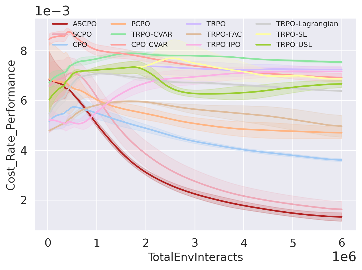
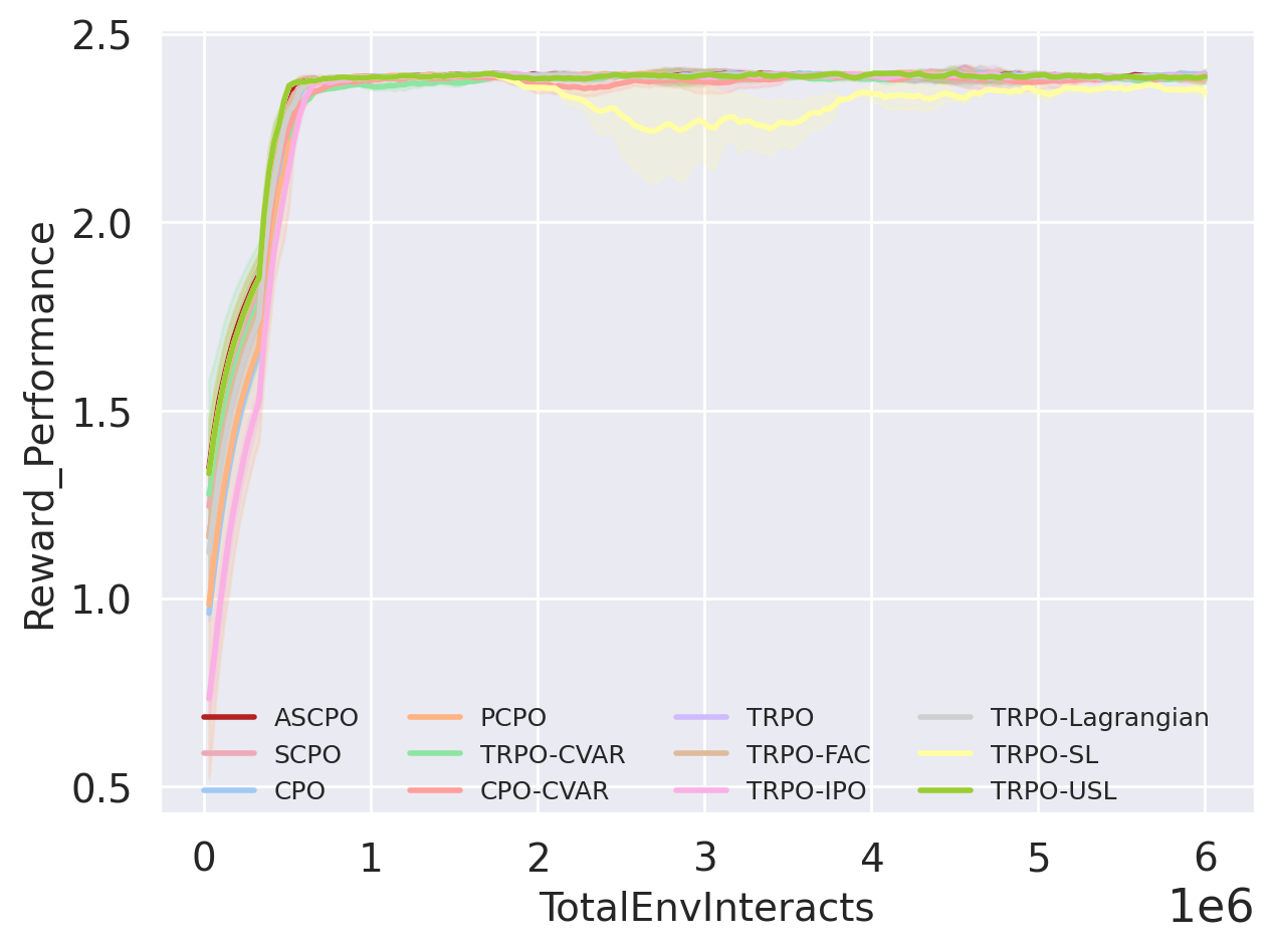
Low Dimensional Systems

We have selected four representative test suites (figs. 9(a), 9(b), 9(c) and 9(d)) to exemplify ASCPO’s performance on low-dimensional systems. The outcomes underscore ASCPO’s remarkable ability to simultaneously achieve near-zero constraint violations and rapid reward convergence, a feat challenging for other algorithms within our comparison group. Specifically, compared to other baseline methods, ASCPO demonstrates: (i) near-zero average episode cost at the swiftest rate, (ii) substantially reduced cost rates, and (iii) stable and expedited reward convergence. Baseline end-to-end CMDP methods (CPO, PCPO, TRPO-Lagrangian, TRPO-FAC, TRPO-IPO) fall short of achieving near-zero cost performance even under a cost limit of zero. Similarly, while SCPO can approach near-zero cost, it exhibits deficiencies in both convergence speed and cost rate reduction, due to fundamental limitation in only regulating expectation in SCMDP methods. Risk-sensitive methods (TRPO-CVaR, CPO-CVaR) prove unsuitable for achieving optimal synthesis and are incapable of nearly zero cost performance. Even with an explicit safety layer correcting unsafe actions at each time step, baseline hierarchical safe RL methods (TRPO-SL, TRPO-USL) fail to achieve near-zero cost performance due to inaccuracies stemming from the linear approximation of the cost function(Dalal et al., 2018) when confronted with highly nonlinear dynamics as encountered in our MuJoCo environments(Todorov et al., 2012). A comprehensive summary of these results is provided in Section B.3.

Practical Systems and High Dimension Systems

To demonstrate the scalability of ASCPO and potential to solve complex robot learning problems, we conducted a series of experiments on practical and high-dimensional systems (figs. 9(e), 9(f), 9(g) and 9(h)). The results underscore ASCPO’s ability to surpass all other algorithms by rapidly achieving both reward and cost convergence while maintaining a remarkably lower cost rate.

It is noteworthy that the PCPO demonstrates superior cost rate reduction performance in the Drone-8Hazards test suite. However, this comes at the expense of intolerably slow and unstable reward increases, rendering it unsuitable for simulation or real-world implementation. In the remaining three test suites, the Lagrangian method exhibits a favorable cost rate performance but concurrently displays poor performance of cost reduction and reward improvement during the early training stages. This discrepancy arises from the robots’ initial struggle to learn task completion and reward optimization, resulting in longer episode lengths and consequently lower cost rates. This significant flaw in the Lagrangian approach underscores its limitations. More details and ablation experiments about Lagrangian method are provided in Section B.4.

Comprehensive Evaluation

To demonstrate the comprehensive ability of our algorithm, we take TRPO as baseline and design a new metric named synthesised score $\psi$ as follow:

\displaystyle\psi_{Current}=\frac{1}{3}\left(\frac{J_{r}^{Current}}{J_{r}^{TRPO}}+\frac{M_{c}^{TRPO}}{M_{c}^{Current}}+\frac{\rho_{c}^{TRPO}}{\rho_{c}^{Current}}\right)

(35)

This metric represents the average improvement magnitude of the current algorithm with respect to TRPO under the three metrics $J_{r}$ , $M_{c}$ and $\rho_{c}$ . It is used to show the comprehensive performance of the safe RL algorithm in a particular task. We averaged the $\psi$ for each of the 12 algorithms across the 19 tasks and present the results in Figure 11. The metrics used for computing can be found in Tables 7(c), 8, 9(c), 10(c), 11(c) and 12(d) in appendix. The results show that our algorithm has a cliff-leading combined effect compared to other algorithms.

Above results demonstrate the superiority of ASCPO in comparison to various other safe RL state-of-the-art methods, which answer Q1.

Absolute Maximum State-wise Cost

In Figure 12, we present a selection of four representative robots across varying dimensions to demonstrate ASCPO’s proficiency in constraining episodic cost values below a specified threshold with exceptionally high probability. We include CPO, CPO-CVaR, SCPO, TRPO, TRPO-FAC and TRPO-Lagrangian as benchmark algorithms for comparison. All algorithms undergo thorough training for 6 million steps, with data collection consisting of 30,000 steps under each of the three random seeds to ensure a robust data distribution. Our analysis reveals that ASCPO not only achieves the lowest mean episodic cost value but also effectively manages the maximum episodic cost, thereby demonstrating ASCPO’s success in controlling the entire distribution with high probability. At the same time, in Figure 13, we take Swimmer-1-Hazard as the representative test suite to concretize the illustration of Figure 1 using real data. The results show that ASCPO can effectively constrain the maximum episodic cost within a safe threshold, demonstrating the superiority of our algorithm in controlling the entire distribution. These results answer Q2.

Ablation on Monotonic-Descent Trick

According to Zhao et al. (Zhao et al., 2024a), algorithms employing the MMDP framework feature cost target functions characterized by step functions, as illustrated in the right panel of Figure 15. These functions delineate the maximum cost increment in any future state relative to the maximal state-wise cost encountered thus far. Consequently, strategies can be employed to enhance the neural network’s fitting of these step functions. A pivotal characteristic of these functions is their monotonically decreasing nature, which informs the design of the loss Equation 34. Moreover, as depicted in Figure 15, the application of the monotonic-descent technique to non-MMDP scenarios (using CPO as an example) appears irrelevant and does not affect their performance. Subsequently, in Figure 18, we demonstrate the impact of employing the monotonic-descent strategy across four test suites. The results demonstrate that this approach accelerates the convergence of cost values towards near-zero values and effectively lowers the cost rate to a desirable level, which answer Q3.

Resources Usage

We conducted comprehensive tests comparing GPU and CPU memory usage, along with wall-clock time, across several algorithms, namely SCPO, CPO, TRPO, TRPO-Lagrangian, and ASCPO. These tests utilized identical system resources in the Goal-8-Hazard task. As illustrated in Figure 20, the results indicate that ASCPO marginally increases GPU and CPU resource consumption compared to CPO and SCPO, while exhibiting nearly identical wall-clock time performance. However, a closer examination of the horizontal coordinate magnitude reveals a significant performance enhancement achieved by ASCPO, requiring less than 1% increase in resources for each aspect. This underscores the effectiveness of our algorithm in delivering exceptional results without imposing substantial demands on system resources and runtime. Furthermore, this observation addresses the pertinent question Q4 regarding the efficacy of our approach.

7 Proximal Absolute State-wise Constrained Policy Optimization

With the proven success of the TRPO-based ASCPO in addressing various control tasks, a natural question arises: Can ASCPO be extended to a PPO-based version, similar to the PPO-Lagrangian implemented in Ray et al. (2019)? To explore this possibility, we introduce PASCPO, which integrates a Clipped Surrogate Objective (Schulman et al., 2017) with the Lagrangian Method Ray et al. (2019). In detail, the original constrained optimization problem within the trust region, as outlined in Algorithm 1, is reformulated as a single-objective optimization problem. The local update is performed using a clipped surrogate objective, while the constraint is incorporated through the Lagrangian method. In Figure 23, we compare our algorithm with fine-tuned PPO-Lagrangian in four representative tasks, demonstrating our effectiveness in achieving lower cost values and more efficient control across the entire distribution. Furthermore, as shown in Figure 25, PASCPO achieves significantly better performance while maintaining essentially the same hardware resource usage and wall-clock time. This demonstrates that our surrogate absolute bound, despite its complexity, does not introduce additional unacceptable computational costs. It is worth noting that PASCPO has significantly higher computing efficiency compared to ASCPO, albeit with some performance loss, making it suitable for specific scenarios. These results address Q5 and highlight the potential of extending ASCPO to a PPO-based method.

8 Conclusion

This paper proposed ASCPO, the first general-purpose policy search algorithm that ensures state-wise constraints satisfaction with high confidence. We demonstrate ASCPO’s effectiveness on challenging continuous control benchmark tasks, showing its significant performance improvement compared to existing methods and ability to handle state-wise constraints.

Acknowledgments and Disclosure of Funding

This work is partially supported by the National Science Foundation, Grant No. 2144489.

Appendix A Additional Proofs

A.1 Proof of 1

Proof According to Selberg’s inequality theory Saw et al. (1984), if random variable $\mathcal{R}_{\pi}(\hat{s}_{0})$ has finite non-zero variance $\mathcal{V}(\pi)$ and finite expected value $\mathcal{E}(\pi)$ . Then for any real number $k\geq 0$ , following inequality holds:

\displaystyle Pr(\mathcal{R}_{\pi}(\hat{s}_{0})>\mathcal{E}(\pi)+k\mathcal{V}(\pi)))\leq\frac{1}{k^{2}\mathcal{V}(\pi)+1}\leavevmode\nobreak\ \leavevmode\nobreak\ \leavevmode\nobreak\ ,

(36)

which equals to:

\displaystyle Pr\big{(}\mathcal{R}_{\pi}(\hat{s}_{0})\leq\mathcal{B}_{k}(\pi)\big{)}\geq 1-\frac{1}{k^{2}\mathcal{V}(\pi)+1}\leavevmode\nobreak\ \leavevmode\nobreak\ \leavevmode\nobreak\ .

(37)

Considering that $\pi\in\Pi$ , then $\mathcal{V}(\pi)$ belongs to a corresponding variance space which has a non-zero minima of $\mathcal{V}(\pi)$ , which is denoted as $\mathcal{V}_{min}\in\mathbb{R}^{+}$ . Therefore, by treating $\psi=\mathcal{V}_{min}$ , the following condition holds:

$\displaystyle\text{There exists $\psi>0$, s.t. }Pr\big{(}\mathcal{R}_{\pi}(\hat{s}_{0})\leq\mathcal{B}_{k}(\pi)\big{)}$	$\displaystyle\geq 1-\frac{1}{k^{2}\mathcal{V}(\pi)+1}$	(38)
	$\displaystyle\geq 1-\frac{1}{k^{2}\mathcal{V}_{min}+1}$
	$\displaystyle=\underbrace{1-\frac{1}{k^{2}\psi+1}}_{p_{k}^{\psi}}\leavevmode\nobreak\ \leavevmode\nobreak\ \leavevmode\nobreak\ .$

A.2 Proof of 3

Proof According to [Finite-horizon Version of Theorem 1, (Sobel, 1982)], the following proposition holds:

Proposition 5

Define $\bm{X}_{\pi}^{H}=\begin{bmatrix}\underset{\begin{subarray}{c}{\hat{\tau}}\sim{\pi}\end{subarray}}{\mathbb{V}ar}[\mathcal{R}_{\pi}^{H}(\hat{s}^{1})]\\ \underset{\begin{subarray}{c}{\hat{\tau}}\sim{\pi}\end{subarray}}{\mathbb{V}ar}[\mathcal{R}_{\pi}^{H}(\hat{s}^{2})]\\ \vdots\end{bmatrix}$ , and ${\hat{P}}_{\pi}=P_{\pi}^{\top}$ , where $\hat{P}_{\pi}(i,j)$ denotes the probability of the transfer from i-th state to j-th state, the following equation holds

\displaystyle\bm{X}_{\pi}^{H}=\gamma^{2}\hat{P}_{\pi}\bm{X}_{\pi}^{H-1}+\bm{\Omega}_{\pi}^{H}

(39)

where $\bm{X}_{\pi}^{0}=\begin{bmatrix}0&0&\ldots\end{bmatrix}^{\top}$ .

With 5, the complete $\bm{X}_{\pi}^{H}$ formula follows immediately

	$\displaystyle\bm{X}_{\pi}^{H}$	$\displaystyle=\bm{\Omega}_{\pi}^{H}+\gamma^{2}\hat{P}_{\pi}\bm{\Omega}_{\pi}^{H-1}+(\gamma^{2}\hat{P}_{\pi})^{2}\bm{\Omega}_{\pi}^{H-2}+\cdots(\gamma^{2}\hat{P}_{\pi})^{H-1}\Omega_{\pi}^{1}$		(40)
		$\displaystyle=\sum_{h=1}^{H}(\gamma^{2}\hat{P}_{\pi})^{H-h}\bm{\Omega}_{\pi}^{h}\leavevmode\nobreak\ \leavevmode\nobreak\ \leavevmode\nobreak\ .$

With (40), The divergence of MeanVariance we want to bound can be written as:

$\displaystyle\|MV_{\pi^{\prime}}-MV_{\pi}\|$	$\displaystyle=\big{\|}\underset{\begin{subarray}{c}\hat{s}_{0}\sim\mu\end{subarray}}{\mathbb{E}}[\underset{\begin{subarray}{c}{\hat{\tau}}\sim{\pi}\end{subarray}}{\mathbb{V}ar}[\mathcal{R}_{\pi^{\prime}}^{H}(\hat{s}_{0})]-\underset{\begin{subarray}{c}\hat{s}_{0}\sim\mu\end{subarray}}{\mathbb{E}}[\underset{\begin{subarray}{c}{\hat{\tau}}\sim{\pi}\end{subarray}}{\mathbb{V}ar}[\mathcal{R}_{\pi}^{H}(\hat{s}_{0})]\big{\|}$	(41)
	$\displaystyle=\\|\mu^{\top}\big{(}\bm{X}_{\pi^{\prime}}^{H}-\bm{X}_{\pi}^{H})\\|_{\infty}$
	$\displaystyle\leq\\|\mu^{\top}\\|_{\infty}\\|\bm{X}_{\pi^{\prime}}^{H}-\bm{X}_{\pi}^{H}\\|_{\infty}$
	$\displaystyle\leq\\|\mu^{\top}\\|_{\infty}\bigg{\\|}\sum_{h=1}^{H}(\gamma^{2}\hat{P}_{\pi^{\prime}})^{H-h}\bm{\Omega}_{\pi^{\prime}}^{h}-\sum_{h=1}^{H}(\gamma^{2}\hat{P}_{\pi})^{H-h}\bm{\Omega}_{\pi}^{h}\bigg{\\|}_{\infty}$
	$\displaystyle\leq\\|\mu^{\top}\\|_{\infty}\sum_{h=1}^{H}\bigg{\\|}(\gamma^{2}\hat{P}_{\pi^{\prime}})^{H-h}\bm{\Omega}_{\pi^{\prime}}^{h}-(\gamma^{2}\hat{P}_{\pi})^{H-h}\bm{\Omega}_{\pi}^{h}\bigg{\\|}_{\infty}\leavevmode\nobreak\ \leavevmode\nobreak\ \leavevmode\nobreak\ \leavevmode\nobreak\ `.$

Next, we will derive the upper bound of $\bigg{\|}(\gamma^{2}\hat{P}_{\pi^{\prime}})^{H-h}\bm{\Omega}_{\pi^{\prime}}^{h}-(\gamma^{2}\hat{P}_{\pi})^{H-h}\bm{\Omega}_{\pi}^{h}\bigg{\|}_{\infty}$

		$\displaystyle\\|(\gamma^{2}\hat{P}_{\pi^{\prime}})^{H-h}\bm{\Omega}_{\pi^{\prime}}^{h}-(\gamma^{2}\hat{P}_{\pi})^{H-h}\bm{\Omega}_{\pi}^{h}\\|_{\infty}$		(42)
		$\displaystyle=\\|(\gamma^{2}\hat{P}_{\pi^{\prime}})^{H-h}\bm{\Omega}_{\pi^{\prime}}^{h}-(\gamma^{2}\hat{P}_{\pi^{\prime}})^{H-h}\bm{\Omega}_{\pi}^{h}+(\gamma^{2}\hat{P}_{\pi^{\prime}})^{H-h}\bm{\Omega}_{\pi}^{h}-(\gamma^{2}\hat{P}_{\pi})^{H-h}\bm{\Omega}_{\pi}^{h}\\|_{\infty}$
		$\displaystyle=\\|(\gamma^{2}\hat{P}_{\pi^{\prime}})^{H-h}\big{(}\bm{\Omega}_{\pi^{\prime}}^{h}-\bm{\Omega}_{\pi}^{h}\big{)}+\big{(}(\gamma^{2}\hat{P}_{\pi^{\prime}})^{H-h}-(\gamma^{2}\hat{P}_{\pi})^{H-h}\big{)}\bm{\Omega}_{\pi}^{h}\\|_{\infty}$
		$\displaystyle\leq\\|(\gamma^{2}\hat{P}_{\pi^{\prime}})^{H-h}\big{(}\bm{\Omega}_{\pi^{\prime}}^{h}-\bm{\Omega}_{\pi}^{h}\big{)}\\|_{\infty}+\\|\big{(}(\gamma^{2}\hat{P}_{\pi^{\prime}})^{H-h}-(\gamma^{2}\hat{P}_{\pi})^{H-h}\big{)}\bm{\Omega}_{\pi}^{h}\\|_{\infty}$
		$\displaystyle\leq\\|(\gamma^{2}\hat{P}_{\pi^{\prime}})^{H-h}\\|_{\infty}\\|\bm{\Omega}_{\pi^{\prime}}^{h}-\bm{\Omega}_{\pi}^{h}\\|_{\infty}+\\|(\gamma^{2}\hat{P}_{\pi^{\prime}})^{H-h}-(\gamma^{2}\hat{P}_{\pi})^{H-h}\\|_{\infty}\\|\bm{\Omega}_{\pi}^{h}\\|_{\infty}$

Since we already know

	$\displaystyle\\|(\gamma^{2}\hat{P}_{\pi^{\prime}})^{H-h}\\|_{\infty}=\|\|\gamma^{2(H-h)}\hat{P}_{\pi^{\prime}}^{H-h}\|\|_{\infty}=\gamma^{2(H-h)},$		(43)
	$\displaystyle{\\|\bm{\Omega}_{\pi}^{h)}\\|_{\infty}}\text{ is a known constant vector given }\pi.$		(44)

We only need to bound $\|\bm{\Omega}_{\pi^{\prime}}^{h}-\bm{\Omega}_{\pi}^{h}\|_{\infty}$ and $\|(\gamma^{2}\hat{P}_{\pi^{\prime}})^{H-h}-(\gamma^{2}\hat{P}_{\pi})^{H-h}\|_{\infty}$ .

To address $\|(\gamma^{2}\hat{P}_{\pi^{\prime}})^{H-h}-(\gamma^{2}\hat{P}_{\pi})^{H-h}\|_{\infty}$ , we have

		$\displaystyle\\|(\gamma^{2}\hat{P}_{\pi^{\prime}})^{H-h}-(\gamma^{2}\hat{P}_{\pi})^{H-h}\\|_{\infty}$		(45)
		$\displaystyle\leq\\|(\gamma^{2}\hat{P}_{\pi^{\prime}})^{H-h}\\|_{\infty}+\\|(\gamma^{2}\hat{P}_{\pi})^{H-h}\\|_{\infty}$
		$\displaystyle=\gamma^{2(H-h)}(\\|\hat{P}_{\pi^{\prime}}^{H-h}\\|_{\infty}+\\|\hat{P}_{\pi}^{H-h}\\|_{\infty})$
		$\displaystyle=2\gamma^{2(H-h)}\leavevmode\nobreak\ \leavevmode\nobreak\ \leavevmode\nobreak\ .$

To address $\|\bm{\Omega}_{\pi^{\prime}}^{h}-\bm{\Omega}_{\pi}^{h}\|_{\infty}$ , we notice that $\omega_{\pi}^{h}(\hat{s})=\underset{\begin{subarray}{c}a\sim\pi\\ \hat{s}^{\prime}\sim P\end{subarray}}{\mathbb{V}ar}[Q_{\pi}^{h}(\hat{s},a,\hat{s}^{\prime})]=\underset{\begin{subarray}{c}a\sim\pi\\ \hat{s}^{\prime}\sim P\end{subarray}}{\mathbb{V}ar}[A_{\pi}^{h}(\hat{s},a,\hat{s}^{\prime})]$ , which means:

\displaystyle\|\bm{\Omega}_{\pi^{\prime}}^{h}-\bm{\Omega}_{\pi}^{h}\|_{\infty}=\underset{\hat{s}}{\mathbf{max}}\bigg{|}\underset{\begin{subarray}{c}a\sim\pi^{\prime}\\ \hat{s}^{\prime}\sim P\end{subarray}}{\mathbb{V}ar}[A_{\pi^{\prime}}^{h}(\hat{s},a,\hat{s}^{\prime})]-\underset{\begin{subarray}{c}a\sim\pi\\ \hat{s}^{\prime}\sim P\end{subarray}}{\mathbb{V}ar}[A_{\pi}^{h}(\hat{s},a,\hat{s}^{\prime})]\bigg{|}

(46)

Where

	$\displaystyle A_{\pi}^{h}(\hat{s},a,\hat{s}^{\prime})$	$\displaystyle=R(\hat{s},a,\hat{s}^{\prime})+\gamma V_{\pi}^{h-1}(\hat{s}^{\prime})-V_{\pi}^{h}(\hat{s})$		(47)
	$\displaystyle A_{\pi^{\prime}}^{h}(\hat{s},a,\hat{s}^{\prime})$	$\displaystyle=R(\hat{s},a,\hat{s}^{\prime})+\gamma V_{\pi^{\prime}}^{h-1}(\hat{s}^{\prime})-V_{\pi^{\prime}}^{h}(\hat{s})$

Define $K^{h}(\hat{s},a,\hat{s}^{\prime})=A_{\pi^{\prime}}^{h}(\hat{s},a,\hat{s}^{\prime})-A_{\pi}^{h}(\hat{s},a,\hat{s}^{\prime})$ , we have:

\displaystyle K^{h}(\hat{s},a,\hat{s}^{\prime})

\displaystyle=\gamma(V_{\pi^{\prime}}^{h-1}(\hat{s}^{\prime})-V_{\pi}^{h-1}(\hat{s}^{\prime}))-(V_{\pi^{\prime}}^{h}(\hat{s})-V_{\pi}^{h}(\hat{s}))

(48)

Similar to TRPO Schulman et al. (2015):

		$\displaystyle\underset{\begin{subarray}{c}\hat{s}_{0}=\hat{s}\\ {\hat{\tau}}\sim\pi^{\prime}\end{subarray}}{\mathbb{E}}\bigg{[}\sum_{t=0}^{h-1}\gamma^{t}A_{\pi}^{h-t}(\hat{s}_{t},a_{t},\hat{s}_{t+1})\bigg{]}$		(49)
		$\displaystyle=\underset{\begin{subarray}{c}\hat{s}_{0}=\hat{s}\\ {\hat{\tau}}\sim\pi^{\prime}\end{subarray}}{\mathbb{E}}\bigg{[}\sum_{t=0}^{h-1}\gamma^{t}(R_{\pi}(\hat{s}_{t},a_{t},\hat{s}_{t+1})+\gamma V_{\pi}^{h-t-1}(\hat{s}_{t+1})-V_{\pi}^{h-t}(\hat{s}_{t}))\bigg{]}$
		$\displaystyle=\underset{\begin{subarray}{c}\hat{s}_{0}=\hat{s}\\ {\hat{\tau}}\sim\pi^{\prime}\end{subarray}}{\mathbb{E}}\bigg{[}-V_{\pi}^{h}(\hat{s}_{0})+\gamma^{h}V_{\pi}^{0}(\hat{s}_{h})+\sum_{t=0}^{h-1}\gamma^{t}R_{\pi}(\hat{s}_{t},a_{t},\hat{s}_{t+1})\bigg{]}$
		$\displaystyle=\underset{\begin{subarray}{c}\hat{s}_{0}=\hat{s}\\ {\hat{\tau}}\sim\pi^{\prime}\end{subarray}}{\mathbb{E}}\bigg{[}-V_{\pi}^{h}(\hat{s}_{0})+\sum_{t=0}^{h-1}\gamma^{t}R_{\pi}(\hat{s}_{t},a_{t},\hat{s}_{t+1})\bigg{]}$
		$\displaystyle=\underset{\begin{subarray}{c}\hat{s}_{0}=\hat{s}\end{subarray}}{\mathbb{E}}\bigg{[}-V_{\pi}^{h}(\hat{s}_{0})\bigg{]}+\underset{\begin{subarray}{c}\hat{s}_{0}=\hat{s}\\ {\hat{\tau}}\sim\pi^{\prime}\end{subarray}}{\mathbb{E}}\bigg{[}\sum_{t=0}^{h-1}\gamma^{t}R_{\pi}(\hat{s}_{t},a_{t},\hat{s}_{t+1})\bigg{]}$
		$\displaystyle=-V_{\pi}^{h}(\hat{s})+V_{\pi^{\prime}}^{h}(\hat{s})$

Then $K^{h}(\hat{s},a,\hat{s}^{\prime})$ can be written as:

\displaystyle K^{h}(\hat{s},a,\hat{s}^{\prime})

\displaystyle=\gamma\underset{\begin{subarray}{c}\hat{s}_{0}=\hat{s}^{\prime}\\ {\hat{\tau}}\sim\pi^{\prime}\end{subarray}}{\mathbb{E}}\bigg{[}\sum_{t=0}^{h-2}\gamma^{t}A_{\pi}^{h-1-t}(\hat{s}_{t},a_{t},\hat{s}_{t+1})\bigg{]}-\underset{\begin{subarray}{c}\hat{s}_{0}=\hat{s}\\ {\hat{\tau}}\sim\pi^{\prime}\end{subarray}}{\mathbb{E}}\bigg{[}\sum_{t=0}^{h-1}\gamma^{t}A_{\pi}^{h-t}(\hat{s}_{t},a_{t},\hat{s}_{t+1})\bigg{]}

(50)

Define ${A_{\pi^{\prime},\pi}^{h}(\hat{s})}$ to be the expected advantage of ${\pi^{\prime}}$ over ${\pi}$ at state ${\hat{s}}$ :

\displaystyle A_{\pi^{\prime},\pi}^{h}(\hat{s})=\underset{a\sim\pi^{\prime}}{\mathbb{E}}\bigg{[}A_{\pi}^{h}(\hat{s},a)\bigg{]}

(51)

Now $K^{h}(\hat{s},a,\hat{s}^{\prime})$ can be written as:

\displaystyle K^{h}(\hat{s},a,\hat{s}^{\prime})

\displaystyle=\gamma\underset{\begin{subarray}{c}\hat{s}_{0}=\hat{s}^{\prime}\\ {\hat{\tau}}\sim\pi^{\prime}\end{subarray}}{\mathbb{E}}\bigg{[}\sum_{t=0}^{h-2}\gamma^{t}A_{\pi^{\prime},\pi}^{h-1-t}(\hat{s}_{t})\bigg{]}-\underset{\begin{subarray}{c}\hat{s}_{0}=\hat{s}\\ {\hat{\tau}}\sim\pi^{\prime}\end{subarray}}{\mathbb{E}}\bigg{[}\sum_{t=0}^{h-1}\gamma^{t}A_{\pi^{\prime},\pi}^{h-t}(\hat{s}_{t})\bigg{]}

(52)

Define ${L(\hat{s},a,\hat{s}^{\prime})}$ as:

\displaystyle L^{h}(\hat{s},a,\hat{s}^{\prime})

\displaystyle=\gamma\underset{\begin{subarray}{c}\hat{s}_{0}=\hat{s}^{\prime}\\ {\hat{\tau}}\sim\pi\end{subarray}}{\mathbb{E}}\bigg{[}\sum_{t=0}^{h-2}\gamma^{t}A_{\pi^{\prime},\pi}^{h-1-t}(\hat{s}_{t})\bigg{]}-\underset{\begin{subarray}{c}\hat{s}_{0}=\hat{s}\\ {\hat{\tau}}\sim\pi\end{subarray}}{\mathbb{E}}\bigg{[}\sum_{t=0}^{h-1}\gamma^{t}A_{\pi^{\prime},\pi}^{h-t}(\hat{s}_{t})\bigg{]}

(53)

With $\epsilon=\underset{\hat{s},a,h}{\mathbf{max}}|A_{\pi}^{h}(\hat{s},a)|$ and the fact that $\big{|}\mathbb{E}_{\hat{s}_{t}\sim\pi^{\prime}}[A^{h}_{\pi^{\prime},\pi}(\hat{s}_{t})]-\mathbb{E}_{\hat{s}_{t}\sim\pi}[A^{h}_{\pi^{\prime},\pi}(\hat{s}_{t})]\big{|}\leq 4\alpha(1-(1-\alpha)^{t})\epsilon$ ([Lemma3, (Schulman et al., 2015)]), where $\alpha=\underset{\hat{s}}{\max}\mathcal{D}_{TV}(\pi^{\prime}\|\pi)[\hat{s}]=\mathcal{D}_{TV}^{max}(\pi^{\prime}\|\pi)$ , we have:

	$\displaystyle\|K^{h}(\hat{s},a,\hat{s}^{\prime})-L^{h}(\hat{s},a,\hat{s}^{\prime})\|$		(54)
	$\displaystyle=\bigg{\|}\gamma\bigg{(}\underset{\begin{subarray}{c}\hat{s}_{0}=\hat{s}^{\prime}\\ {\hat{\tau}}\sim\pi^{\prime}\end{subarray}}{\mathbb{E}}\bigg{[}\sum_{t=0}^{h-2}\gamma^{t}A_{\pi^{\prime},\pi}^{h-1-t}(\hat{s}_{t})\bigg{]}-\underset{\begin{subarray}{c}\hat{s}_{0}=\hat{s}^{\prime}\\ {\hat{\tau}}\sim\pi\end{subarray}}{\mathbb{E}}\bigg{[}\sum_{t=0}^{h-2}\gamma^{t}A_{\pi^{\prime},\pi}^{h-1-t}(\hat{s}_{t})\bigg{]}\bigg{)}$
	$\displaystyle-\bigg{(}\underset{\begin{subarray}{c}\hat{s}_{0}=\hat{s}\\ {\hat{\tau}}\sim\pi^{\prime}\end{subarray}}{\mathbb{E}}\bigg{[}\sum_{t=0}^{h-1}\gamma^{t}A_{\pi^{\prime},\pi}^{h-t}(\hat{s}_{t})\bigg{]}-\underset{\begin{subarray}{c}\hat{s}_{0}=\hat{s}\\ {\hat{\tau}}\sim\pi\end{subarray}}{\mathbb{E}}\bigg{[}\sum_{t=0}^{h-1}\gamma^{t}A_{\pi^{\prime},\pi}^{h-t}(\hat{s}_{t})\bigg{]}\bigg{)}\bigg{\|}$
	$\displaystyle\leq\gamma\bigg{\|}\underset{\begin{subarray}{c}\hat{s}_{0}=\hat{s}^{\prime}\\ {\hat{\tau}}\sim\pi^{\prime}\end{subarray}}{\mathbb{E}}\bigg{[}\sum_{t=0}^{h-2}\gamma^{t}A_{\pi^{\prime},\pi}^{h-1-t}(\hat{s}_{t})\bigg{]}-\underset{\begin{subarray}{c}\hat{s}_{0}=\hat{s}^{\prime}\\ {\hat{\tau}}\sim\pi\end{subarray}}{\mathbb{E}}\bigg{[}\sum_{t=0}^{h-2}\gamma^{t}A_{\pi^{\prime},\pi}^{h-1-t}(\hat{s}_{t})\bigg{]}\bigg{\|}$
	$\displaystyle+\bigg{\|}\underset{\begin{subarray}{c}\hat{s}_{0}=\hat{s}\\ {\hat{\tau}}\sim\pi^{\prime}\end{subarray}}{\mathbb{E}}\bigg{[}\sum_{t=0}^{h-1}\gamma^{t}A_{\pi^{\prime},\pi}^{h-t}(\hat{s}_{t})\bigg{]}-\underset{\begin{subarray}{c}\hat{s}_{0}=\hat{s}\\ {\hat{\tau}}\sim\pi\end{subarray}}{\mathbb{E}}\bigg{[}\sum_{t=0}^{h-1}\gamma^{t}A_{\pi^{\prime},\pi}^{h-t}(\hat{s}_{t})\bigg{]}\bigg{\|}$
	$\displaystyle\leq 4\epsilon\alpha\bigg{(}\gamma\frac{1-\gamma^{h-2}}{1-\gamma}-\gamma\frac{1-\gamma^{h-2}(1-\alpha)^{h-2}}{1-\gamma(1-\alpha)}+\frac{1-\gamma^{h-1}}{1-\gamma}-\frac{1-\gamma^{h-1}(1-\alpha)^{h-1}}{1-\gamma(1-\alpha)}\bigg{)}$
	$\displaystyle\leq\frac{8\epsilon(\gamma-\gamma^{h})}{(1-\gamma)^{2}}(\mathcal{D}_{TV}^{max}(\pi^{\prime}\\|\pi))^{2}$

Then according to Brillinger (2018) $\mathcal{D}_{TV}(\pi^{\prime}\|\pi)[\hat{s}]\leq\sqrt{\frac{1}{2}\mathcal{D}_{KL}(\pi^{\prime}\|\pi)[\hat{s}]}$ , we can then bound ${|K(\hat{s},a,\hat{s}^{\prime})|}$ with:

	$\displaystyle\|K^{h}(\hat{s},a,\hat{s}^{\prime})\|$	$\displaystyle\leq\left\|L^{h}(\hat{s},a,\hat{s}^{\prime})\right\|+\frac{8\epsilon(\gamma-\gamma^{h})}{(1-\gamma)^{2}}(\mathcal{D}_{TV}^{max}(\pi^{\prime}\\|\pi))^{2}$		(55)
		$\displaystyle\leq\left\|L^{h}(\hat{s},a,\hat{s}^{\prime})\right\|+\frac{4\epsilon(\gamma-\gamma^{h})}{(1-\gamma)^{2}}\mathcal{D}_{KL}^{max}(\pi^{\prime}\\|\pi)\doteq\|K^{h}(\hat{s},a,\hat{s}^{\prime})\|_{max}$

where $\mathcal{D}_{KL}^{max}(\pi^{\prime}\|\pi)=\max_{s}\mathcal{D}_{KL}(\pi^{\prime}\|\pi)[s]$ . With $A_{\pi^{\prime}}^{h}(\hat{s},a,\hat{s}^{\prime})=A_{\pi}^{h}(\hat{s},a,\hat{s}^{\prime})+K^{h}(\hat{s},a,\hat{s}^{\prime})$ , we have:

	$\displaystyle\underset{\begin{subarray}{c}a\sim\pi^{\prime}\\ \hat{s}^{\prime}\sim P\end{subarray}}{\mathbb{V}ar}[A_{\pi^{\prime}}^{h}(\hat{s},a,\hat{s}^{\prime})]-\underset{\begin{subarray}{c}a\sim\pi\\ \hat{s}^{\prime}\sim P\end{subarray}}{\mathbb{V}ar}[A_{\pi}^{h}(\hat{s},a,\hat{s}^{\prime})]$	(56)
$\displaystyle=$	$\displaystyle\underset{\begin{subarray}{c}a\sim\pi^{\prime}\\ \hat{s}^{\prime}\sim P\end{subarray}}{\mathbb{E}}[A_{\pi^{\prime}}^{h}(\hat{s},a,\hat{s}^{\prime})^{2}]-\underset{\begin{subarray}{c}a\sim\pi\\ \hat{s}^{\prime}\sim P\end{subarray}}{\mathbb{E}}[A_{\pi}^{h}(\hat{s},a,\hat{s}^{\prime})^{2}]$
$\displaystyle=$	$\displaystyle\underset{\begin{subarray}{c}a\sim\pi^{\prime}\\ \hat{s}^{\prime}\sim P\end{subarray}}{\mathbb{E}}[(A_{\pi}^{h}(\hat{s},a,\hat{s}^{\prime})+K^{h}(\hat{s},a,\hat{s}^{\prime}))^{2}]-\underset{\begin{subarray}{c}a\sim\pi\\ \hat{s}^{\prime}\sim P\end{subarray}}{\mathbb{E}}[A_{\pi}^{h}(\hat{s},a,\hat{s}^{\prime})^{2}]$
$\displaystyle=$	$\displaystyle\underset{\begin{subarray}{c}a\sim\pi^{\prime}\\ \hat{s}^{\prime}\sim P\end{subarray}}{\mathbb{E}}[A_{\pi}^{h}(\hat{s},a,\hat{s}^{\prime})^{2}]-\underset{\begin{subarray}{c}a\sim\pi\\ \hat{s}^{\prime}\sim P\end{subarray}}{\mathbb{E}}[A_{\pi}^{h}(\hat{s},a,\hat{s}^{\prime})^{2}]+2\underset{\begin{subarray}{c}a\sim\pi^{\prime}\\ \hat{s}^{\prime}\sim P\end{subarray}}{\mathbb{E}}[A_{\pi}(\hat{s},a,\hat{s}^{\prime})K^{h}(\hat{s},a,\hat{s}^{\prime})]+\underset{\begin{subarray}{c}a\sim\pi^{\prime}\\ \hat{s}^{\prime}\sim P\end{subarray}}{\mathbb{E}}[K^{h}(\hat{s},a,\hat{s}^{\prime})^{2}]$
$\displaystyle=$	$\displaystyle\underset{\begin{subarray}{c}\\ a\sim\pi\\ \hat{s}^{\prime}\sim P\end{subarray}}{\mathbb{E}}\left[\left(\frac{\pi^{\prime}(a\|\hat{s})}{\pi(a\|\hat{s})}-1\right)A_{\pi}^{h}(\hat{s},a,\hat{s}^{\prime})^{2}\right]+2\underset{\begin{subarray}{c}a\sim\pi^{\prime}\\ \hat{s}^{\prime}\sim P\end{subarray}}{\mathbb{E}}[A_{\pi}^{h}(\hat{s},a,\hat{s}^{\prime})K^{h}(\hat{s},a,\hat{s}^{\prime})]+\underset{\begin{subarray}{c}a\sim\pi^{\prime}\\ \hat{s}^{\prime}\sim P\end{subarray}}{\mathbb{E}}[K^{h}(\hat{s},a,\hat{s}^{\prime})^{2}]$
	$\displaystyle\leq\underset{\begin{subarray}{c}\\ a\sim\pi\\ \hat{s}^{\prime}\sim P\end{subarray}}{\mathbb{E}}\left[\left(\frac{\pi^{\prime}(a\|\hat{s})}{\pi(a\|\hat{s})}-1\right)A_{\pi}^{h}(\hat{s},a,\hat{s}^{\prime})^{2}+2\left(\frac{\pi^{\prime}(a\|\hat{s})}{\pi(a\|\hat{s})}\right)A_{\pi}^{h}(\hat{s},a,\hat{s}^{\prime})\|K^{h}(\hat{s},a,\hat{s}^{\prime})\|_{max}+\|K^{h}(\hat{s},a,\hat{s}^{\prime})\|_{max}^{2}\right]$

Then we can bound ${\|\bm{\Omega}_{\pi^{\prime}}-\bm{\Omega}_{\pi}\|_{\infty}}$ with:

		$\displaystyle\\|\bm{\Omega}_{\pi^{\prime}}-\bm{\Omega}_{\pi}\\|_{\infty}$		(57)
		$\displaystyle\leq\underset{\hat{s}}{\mathbf{max}}\bigg{\|}\underset{\begin{subarray}{c}\\ a\sim\pi\\ \hat{s}^{\prime}\sim P\end{subarray}}{\mathbb{E}}\bigg{[}\left(\frac{\pi^{\prime}(a\|\hat{s})}{\pi(a\|\hat{s})}-1\right)A_{\pi}^{h}(\hat{s},a,\hat{s}^{\prime})^{2}$
		$\displaystyle\leavevmode\nobreak\ \leavevmode\nobreak\ \leavevmode\nobreak\ \leavevmode\nobreak\ \leavevmode\nobreak\ +2\left(\frac{\pi^{\prime}(a\|\hat{s})}{\pi(a\|\hat{s})}\right)A_{\pi}^{h}(\hat{s},a,\hat{s}^{\prime})\|K^{h}(\hat{s},a,\hat{s}^{\prime})\|_{max}+\|K^{h}(\hat{s},a,\hat{s}^{\prime})\|_{max}^{2}\bigg{]}\bigg{\|}$

By substituting (43), (44), (45) and (57) into Equation 42, we have:

	$\displaystyle\\|(\gamma^{2}\hat{P}_{\pi^{\prime}})^{H-h}\bm{\Omega}_{\pi^{\prime}}^{h}-(\gamma^{2}P_{\pi})^{H-h}\bm{\Omega}_{\pi}^{h}\\|_{1}$		(58)
	$\displaystyle\leq\gamma^{2(H-h)}\underset{\hat{s}}{\mathbf{max}}\bigg{\|}\underset{\begin{subarray}{c}\\ a\sim\pi\\ \hat{s}^{\prime}\sim P\end{subarray}}{\mathbb{E}}\bigg{[}\left(\frac{\pi^{\prime}(a\|\hat{s})}{\pi(a\|\hat{s})}-1\right)A_{\pi}^{h}(\hat{s},a,\hat{s}^{\prime})^{2}$
	$\displaystyle\leavevmode\nobreak\ \leavevmode\nobreak\ \leavevmode\nobreak\ \leavevmode\nobreak\ \leavevmode\nobreak\ +2\left(\frac{\pi^{\prime}(a\|\hat{s})}{\pi(a\|\hat{s})}\right)A_{\pi}^{h}(\hat{s},a,\hat{s}^{\prime})\|K^{h}(\hat{s},a,\hat{s}^{\prime})\|_{max}+\|K^{h}(\hat{s},a,\hat{s}^{\prime})\|_{max}^{2}\bigg{]}\bigg{\|}+2\gamma^{2(H-h)}\\|\bm{\Omega}_{\pi}^{h}\\|_{\infty}$

By substituting (58) into (41), 3 is proved.

A.3 Proof of 4

Proof

\displaystyle VM_{\pi^{\prime}}=\underset{\hat{s}_{0}\sim\mu}{\mathbb{E}}[(V^{H}_{\pi^{\prime}}(\hat{s}_{0}))^{2}]-\mathcal{E}(\pi^{\prime})^{2}

(59)

Since both terms on the right of Equation 59 are non-negative, we can bound $VM_{\pi^{\prime}}$ with the upper bound of $\underset{\hat{s}_{0}\sim\mu}{\mathbb{E}}[(V_{\pi^{\prime}}^{H}(\hat{s}_{0}))^{2}]$ and the lower bound of $\mathcal{E}(\pi^{\prime})^{2}$ .
Define $\bm{Y}_{\pi}=\begin{bmatrix}(V_{\pi}^{H}(\hat{s}^{1}))^{2}\\ (V_{\pi}^{H}(\hat{s}^{2}))^{2}\\ \vdots\end{bmatrix}$ , where $\underset{\hat{s}_{0}\sim\mu}{\mathbb{E}}[(V_{\pi}^{H}(\hat{s}_{0}))^{2}]=\mu^{\top}\bm{Y}_{\pi}$ . Then we have

		$\displaystyle\big{\|}\underset{\hat{s}_{0}\sim\mu}{\mathbb{E}}[(V_{\pi^{\prime}}^{H}(\hat{s}_{0}))^{2}]-\underset{\hat{s}_{0}\sim\mu}{\mathbb{E}}[(V_{\pi}^{H}(\hat{s}_{0}))^{2}]\big{\|}$		(60)
		$\displaystyle=\\|\mu^{\top}\big{(}\bm{Y}_{\pi^{\prime}}-\bm{Y}_{\pi})\\|_{\infty}$
		$\displaystyle\leq\\|\mu^{\top}\\|_{\infty}\\|\bm{Y}_{\pi^{\prime}}-\bm{Y}_{\pi}\\|_{\infty}$

To address $\|\bm{Y}_{\pi^{\prime}}-\bm{Y}_{\pi}\|_{\infty}$ , we have:

\displaystyle(V_{\pi^{\prime}}^{H}(\hat{s}))^{2}-(V_{\pi}^{H}(\hat{s}))^{2}

\displaystyle=\bigg{(}V^{H}_{\pi^{\prime}}(\hat{s})-V^{H}_{\pi}(\hat{s})\bigg{)}\bigg{(}V^{H}_{\pi^{\prime}}(\hat{s})+V^{H}_{\pi}(\hat{s})\bigg{)}

(61)

According to (49):

$\displaystyle V^{H}_{\pi^{\prime}}(\hat{s})-V^{H}_{\pi}(\hat{s})$	$\displaystyle=\underset{\begin{subarray}{c}\hat{s}_{0}=\hat{s}\\ {\hat{\tau}}\sim\pi^{\prime}\end{subarray}}{\mathbb{E}}\bigg{[}\sum_{t=0}^{H-1}\gamma^{t}A^{H-t}_{\pi}(\hat{s}_{t},a_{t},\hat{s}_{t+1})\bigg{]}$	(62)
	$\displaystyle=\underset{\begin{subarray}{c}\hat{s}_{0}=\hat{s}\\ {\hat{\tau}}\sim\pi^{\prime}\end{subarray}}{\mathbb{E}}\bigg{[}\sum_{t=0}^{H-1}\gamma^{t}\bar{A}^{H-t}_{\pi^{\prime},\pi}(\hat{s}_{t})\bigg{]}$
	$\displaystyle\dot{=}\ \ \eta(\hat{s})$

Define $L(\hat{s})=\underset{\begin{subarray}{c}\hat{s}_{0}=\hat{s}\\ {\hat{\tau}}\sim\pi\end{subarray}}{\mathbb{E}}\bigg{[}\sum_{t=0}^{H-1}\gamma^{t}\bar{A}^{H-t}_{\pi^{\prime},\pi}(\hat{s}_{t})\bigg{]}$ , then we have:

$\displaystyle\|\eta(\hat{s})-L(\hat{s})\|$	$\displaystyle=\bigg{\|}\underset{\begin{subarray}{c}\hat{s}_{0}=\hat{s}\\ {\hat{\tau}}\sim\pi^{\prime}\end{subarray}}{\mathbb{E}}\bigg{[}\sum_{t=0}^{H-1}\gamma^{t}\bar{A}^{H-t}_{\pi^{\prime},\pi}(\hat{s}_{t})\bigg{]}-\underset{\begin{subarray}{c}\hat{s}_{0}=\hat{s}\\ {\hat{\tau}}\sim\pi\end{subarray}}{\mathbb{E}}\bigg{[}\sum_{t=0}^{H-1}\gamma^{t}\bar{A}^{H-t}_{\pi^{\prime},\pi}(\hat{s}_{t})\bigg{]}\bigg{\|}$	(63)
	$\displaystyle\leq 4\epsilon\alpha\left(\frac{1-\gamma^{H-1}}{1-\gamma}-\frac{1-\gamma^{H-1}(1-\alpha)^{H-1}}{1-\gamma(1-\alpha)}\right)$
	$\displaystyle\leq\frac{4\epsilon(\gamma-\gamma^{H})}{(1-\gamma)^{2}}(\mathcal{D}_{TV}(\pi^{\prime}\\|\pi)[\hat{s}])^{2}$

And according to Brillinger (2018), we can bound $|\eta(\hat{s})|$ with:

	$\displaystyle\|\eta(\hat{s})\|$	$\displaystyle\leq\left\|L(\hat{s})\right\|+\frac{4\epsilon(\gamma-\gamma^{H})}{(1-\gamma)^{2}}(\mathcal{D}_{TV}(\pi^{\prime}\\|\pi)[\hat{s}])^{2}$		(64)
		$\displaystyle\leq\left\|L(\hat{s})\right\|+\frac{2\epsilon(\gamma-\gamma^{H})}{(1-\gamma)^{2}}\mathcal{D}^{max}_{KL}(\pi^{\prime}\\|\pi)\doteq\|\eta(\hat{s})\|_{max}$

Further, we can obtain:

$\displaystyle\|V^{H}_{\pi^{\prime}}(\hat{s})+V^{H}_{\pi}(\hat{s})\|$	$\displaystyle\leq\|V^{H}_{\pi^{\prime}}(\hat{s})\|+\|V^{H}_{\pi}(\hat{s})\|$	(65)
	$\displaystyle=\|V^{H}_{\pi^{\prime}}(\hat{s})\|-\|V^{H}_{\pi}(\hat{s})\|+2\|V^{H}_{\pi}(\hat{s})\|$
	$\displaystyle\leq\|V^{H}_{\pi^{\prime}}(\hat{s})-V^{H}_{\pi}(\hat{s})\|+2\|V^{H}_{\pi}(\hat{s})\|$
	$\displaystyle\leq\|\eta(\hat{s})\|_{max}+2\|V^{H}_{\pi}(\hat{s})\|$

Thus the following inequality holds:

		$\displaystyle\\|\bm{Y}_{\pi^{\prime}}-\bm{Y}_{\pi}\\|_{\infty}$		(66)
		$\displaystyle\leq\underset{\hat{s}}{\mathbf{max}}\bigg{\|}\|V^{H}_{\pi^{\prime}}(\hat{s})-V^{H}_{\pi}(\hat{s})\|\cdot\|V^{H}_{\pi^{\prime}}(\hat{s})+V^{H}_{\pi}(\hat{s})\|\bigg{\|}$
		$\displaystyle\leq\underset{\hat{s}}{\mathbf{max}}\bigg{\|}\|\eta(\hat{s})\|_{max}\cdot\left(\|\eta(\hat{s})\|_{max}+2\|V^{H}_{\pi}(\hat{s})\|\right)\bigg{\|}$
		$\displaystyle=\underset{\hat{s}}{\mathbf{max}}\bigg{\|}\|\eta(\hat{s})\|_{max}^{2}+2\|V^{H}_{\pi}(\hat{s})\|\cdot\|\eta(\hat{s})\|_{max}\bigg{\|}$

Substitute Equation 66 into Equation 60 the upper bound of $\underset{\hat{s}_{0}\sim\mu}{\mathbb{E}}[(V_{\pi^{\prime}}^{H}(\hat{s}_{0}))^{2}]$ is obtained:

\displaystyle\underset{\hat{s}_{0}\sim\mu}{\mathbb{E}}[(V_{\pi^{\prime}}^{H}(\hat{s}_{0}))^{2}]

\displaystyle\leq\underset{\hat{s}_{0}\sim\mu}{\mathbb{E}}[(V^{H}_{\pi}(\hat{s}_{0}))^{2}]+\|\mu^{T}\|_{\infty}\underset{\hat{s}}{\mathbf{max}}\bigg{|}|\eta(\hat{s})|_{max}^{2}+2|V^{H}_{\pi}(\hat{s})|\cdot|\eta(\hat{s})|_{max}\bigg{|}

(67)

The lower bound of $\mathcal{E}(\pi^{\prime})^{2}$ can then be obtained according to (Zhao et al., 2024a):

\displaystyle\mathcal{E}(\pi^{\prime})^{2}\geq\left(\mathbf{min}\left\{\mathbf{max}\left\{0,\ \mathcal{E}^{l}_{\pi^{\prime},\pi}\right\},\mathcal{E}^{u}_{\pi^{\prime},\pi}\right\}\right)^{2}

(68)

where

	$\displaystyle\mathcal{E}^{l}_{\pi^{\prime},\pi}$	$\displaystyle=\mathcal{E}(\pi)+\underset{\begin{subarray}{c}\hat{s}\sim\overline{d}_{\pi}\\ a\sim{\pi^{\prime}}\end{subarray}}{\mathbb{E}}\bigg{[}A^{H}_{\pi}(\hat{s},a)-2(H+1)\epsilon^{\pi^{\prime}}\sqrt{\frac{1}{2}\mathcal{D}_{KL}({\pi^{\prime}}\\|\pi)[\hat{s}]}\bigg{]}$
	$\displaystyle\mathcal{E}^{u}_{\pi^{\prime},\pi}$	$\displaystyle=\mathcal{E}(\pi)+\underset{\begin{subarray}{c}\hat{s}\sim\overline{d}_{\pi}\\ a\sim{\pi^{\prime}}\end{subarray}}{\mathbb{E}}\bigg{[}A^{H}_{\pi}(\hat{s},a)+2(H+1)\epsilon^{\pi^{\prime}}\sqrt{\frac{1}{2}\mathcal{D}_{KL}({\pi^{\prime}}\\|\pi)[\hat{s}]}\bigg{]}$
	$\displaystyle\overline{d}_{\pi}$	$\displaystyle=\sum\limits_{t=0}^{H}P(\hat{s}_{t}=\hat{s}\|\pi)$

By substituting Equation 67 and Equation 68 into Equation 59 4 is proved.

Appendix B Experiment Details

B.1 Environment Settings

Goal Task

In the Goal task environments, the reward function is:

\begin{split}&r(x_{t})=d^{g}_{t-1}-d^{g}_{t}+\mathbf{1}[d^{g}_{t}<R^{g}]\leavevmode\nobreak\ ,\\ \end{split}

where $d^{g}_{t}$ is the distance from the robot to its closest goal and $R^{g}$ is the size (radius) of the goal. When a goal is achieved, the goal location is randomly reset to someplace new while keeping the rest of the layout the same. The test suites of our experiments are summarized in Table 3.

Table 3: The test suites environments of our experiments

	Ground robot						Aerial robot
Task Setting	Low dimension			High dimension
	Point	Swimmer	Arm3	Humanoid	Ant	Walker	Drone
1-Hazard	✓	✓
4-Hazard	✓	✓
8-Hazard	✓	✓	✓	✓	✓	✓
1-Pillar	✓
4-Pillar	✓
8-Pillar	✓
1-Ghost	✓
4-Ghost	✓
8-Ghost	✓
3DHazard-1							✓
3DHazard-4							✓
3DHazard-8							✓

Hazard Constraint

In the Hazard constraint environments, the cost function is:

\begin{split}&c(x_{t})=\max(0,R^{h}-d^{h}_{t})\leavevmode\nobreak\ ,\\ \end{split}

where $d^{h}_{t}$ is the distance to the closest hazard and $R^{h}$ is the size (radius) of the hazard.

Pillar Constraint

In the Pillar constraint environments, the cost $c_{t}=1$ if the robot contacts with the pillar otherwise $c_{t}=0$ .

Ghost Constraint

In the Ghost constraint environments, the cost function is:

\begin{split}&c(x_{t})=\max(0,R^{h}-d^{h}_{t})\leavevmode\nobreak\ ,\\ \end{split}

where $d^{h}_{t}$ is the distance to the closest ghost and $R^{h}$ is the size (radius) of the ghost. And dynamics of ghosts are as follow:

\dot{x}_{object}=\begin{cases}\begin{aligned} v_{0}*&d_{origin},&\text{if }&\left\|d_{origin}\right\|>r_{0}\\ v_{1}*&d_{robot},&\text{if }&\left\|d_{origin}\right\|\leq r_{0}\text{ and }\left\|d_{robot}\right\|>r_{1}\\ &0,&\text{if }&\left\|d_{origin}\right\|\leq r_{0}\text{ and }\left\|d_{robot}\right\|\leq r_{1}\\ \end{aligned}\end{cases},

(69)

where $d_{\text{origin}}=x_{\text{origin}}-x_{\text{object}}$ represents the distance from the position of the dynamic object $x_{\text{object}}$ , $d_{\text{robot}}=x_{\text{robot}}-x_{\text{object}}$ represents the distance from the dynamic object $x_{\text{object}}$ to the position of the robot $x_{\text{robot}}$ , $r_{0}$ defines a circular area centered at the origin point within which the objects are limited to move. $r_{1}$ represents the threshold distance that the dynamic objects strive to maintain from the robot and $v_{0}$ , $v_{1}$ are configurable non-negative velocity constants for the dynamic objects.

State Space

The state space is composed of two parts. The internal state spaces describe the state of the robots, which can be obtained from standard robot sensors (accelerometer, gyroscope, magnetometer, velocimeter, joint position sensor, joint velocity sensor and touch sensor). The details of the internal state spaces of the robots in our test suites are summarized in Table 4. The external state spaces are describe the state of the environment observed by the robots, which can be obtained from 2D lidar or 3D lidar (where each lidar sensor perceives objects of a single kind). The state spaces of all the test suites are summarized in Table 5. Note that Vase and Gremlin are two other constraints in Safety Gym (Ray et al., 2019) and all the returns of vase lidar and gremlin lidar are zero vectors (i.e., $[0,0,\cdots,0]\in\mathbb{R}^{16}$ ) in our experiments since none of our test suites environments has vases.

Table 4: The internal state space components of different test suites environments.

Internal State Space	Point	Swimmer	Walker	Ant	Drone	Arm3	Humanoid
Accelerometer ( $\mathbb{R}^{3}$ )	✓	✓	✓	✓	✓	✓ $\times 5$	✓
Gyroscope ( $\mathbb{R}^{3}$ )	✓	✓	✓	✓	✓	✓ $\times 5$	✓
Magnetometer ( $\mathbb{R}^{3}$ )	✓	✓	✓	✓	✓	✓ $\times 5$	✓
Velocimeter ( $\mathbb{R}^{3}$ )	✓	✓	✓	✓	✓	✓ $\times 5$	✓
Joint position sensor ( $\mathbb{R}^{n}$ )	${n=0}$	${n=2}$	${n=10}$	${n=8}$	${n=0}$	${n=3}$	${n=17}$
Joint velocity sensor ( $\mathbb{R}^{n}$ )	${n=0}$	${n=2}$	${n=10}$	${n=8}$	${n=0}$	${n=3}$	${n=17}$
Touch sensor ( $\mathbb{R}^{n}$ )	${n=0}$	${n=4}$	${n=2}$	${n=8}$	${n=0}$	${n=1}$	${n=2}$

Table 5: The external state space components of different test suites environments.

External State Space	Goal-Hazard	3D-Goal-Hazard	Goal-Pillar
Goal Compass ( $\mathbb{R}^{3}$ )	✓	✓	✓
Goal Lidar ( $\mathbb{R}^{16}$ )	✓	$\times$	✓
3D Goal Lidar ( $\mathbb{R}^{60}$ )	$\times$	✓	$\times$
Hazard Lidar ( $\mathbb{R}^{16}$ )	✓	$\times$	$\times$
3D Hazard Lidar ( $\mathbb{R}^{60}$ )	$\times$	✓	$\times$
Pillar Lidar ( $\mathbb{R}^{16}$ )	$\times$	$\times$	✓
Vase Lidar ( $\mathbb{R}^{16}$ )	✓	$\times$	✓
Gremlin Lidar ( $\mathbb{R}^{16}$ )	✓	$\times$	✓

Control Space

For all the experiments, the control space of all robots are continuous, and linearly scaled to [-1, +1].

B.2 Policy Settings

The hyper-parameters used in our experiments are listed in Table 6 as default.

Our experiments use separate multi-layer perception with ${tanh}$ activations for the policy network, value network and cost network. Each network consists of two hidden layers of size (64,64). All of the networks are trained using $Adam$ optimizer with learning rate of 0.01.

We apply an on-policy framework in our experiments. During each epoch the agent interact $B$ times with the environment and then perform a policy update based on the experience collected from the current epoch. The maximum length of the trajectory is set to 1000 and the total epoch number $N$ is set to 200 as default.

The policy update step is based on the scheme of TRPO, which performs up to 100 steps of backtracking with a coefficient of 0.8 for line searching.

For all experiments, we use a discount factor of $\gamma=0.99$ , an advantage discount factor $\lambda=0.95$ , and a KL-divergence step size of $\delta_{KL}=0.02$ .

For experiments which consider cost constraints we adopt a target cost $\delta_{c}=0.0$ to pursue a zero-violation policy.

Other unique hyper-parameters for each algorithms are hand-tuned to attain reasonable performance.

Each model is trained on a server with a 48-core Intel(R) Xeon(R) Silver 6426Y CPU @ 2.5.GHz, Nvidia RTX A6000 GPU with 48GB memory, and Ubuntu 22.04.

For all tasks, we train each model for 6e6 steps which takes around seven hours.

Table 6: Important hyper-parameters of different algorithms in our experiments

Policy Parameter		TRPO	TRPO-Lagrangian	TRPO-SL [18’ Dalal]	TRPO-USL	TRPO-IPO	TRPO-FAC	CPO	PCPO	SCPO	TRO-CVaR	CPO-CVaR	ASCPO
Epochs	$N$	200	200	200	200	200	200	200	200	200	200	200	200
Steps per epoch	$B$	30000	30000	30000	30000	30000	30000	30000	30000	30000	30000	30000	30000
Maximum length of trajectory	$L$	1000	1000	1000	1000	1000	1000	1000	1000	1000	1000	1000	1000
Policy network hidden layers		(64, 64)	(64, 64)	(64, 64)	(64, 64)	(64, 64)	(64, 64)	(64, 64)	(64, 64)	(64, 64)	(64, 64)	(64, 64)	(64, 64)
Discount factor	$\gamma$	0.99	0.99	0.99	0.99	0.99	0.99	0.99	0.99	0.99	0.99	0.99	0.99
Advantage discount factor	$\lambda$	0.97	0.97	0.97	0.97	0.97	0.97	0.97	0.97	0.97	0.97	0.97	0.97
TRPO backtracking steps		100	100	100	100	100	100	100	-	100	100	100	100
TRPO backtracking coefficient		0.8	0.8	0.8	0.8	0.8	0.8	0.8	-	0.8	0.8	0.8	0.8
Target KL	$\delta_{KL}$	0.02	0.02	0.02	0.02	0.02	0.02	0.02	0.02	0.02	0.02	0.02	0.02
Value network hidden layers		(64, 64)	(64, 64)	(64, 64)	(64, 64)	(64, 64)	(64, 64)	(64, 64)	(64, 64)	(64, 64)	(64, 64)	(64, 64)	(64, 64)
Value network iteration		80	80	80	80	80	80	80	80	80	80	80	80
Value network optimizer		Adam	Adam	Adam	Adam	Adam	Adam	Adam	Adam	Adam	Adam	Adam	Adam
Value learning rate		0.001	0.001	0.001	0.001	0.001	0.001	0.001	0.001	0.001	0.001	0.001	0.001
Cost network hidden layers		-	(64, 64)	(64, 64)	(64, 64)	-	(64, 64)	(64, 64)	(64, 64)	(64, 64)	(64, 64)	(64, 64)	(64, 64)
Cost network iteration		-	80	80	80	-	80	80	80	80	80	80	80
Cost network optimizer		-	Adam	Adam	Adam	-	Adam	Adam	Adam	Adam	Adam	Adam	Adam
Cost learning rate		-	0.001	0.001	0.001	-	0.001	0.001	0.001	0.001	0.001	0.001	0.001
Target Cost	$\delta_{c}$	-	0.0	0.0	0.0	0.0	0.0	0.0	0.0	0.0	0.0	0.0	0.0
Lagrangian optimizer		-	-	-	-	-	Adam	-	-	-	-	-	-
Lagrangian learning rate		-	0.005	-	-	-	0.0001	-	-	-	-	-	-
USL correction iteration		-	-	-	20	-	-	-	-	-	-	-	-
USL correction rate		-	-	-	0.05	-	-	-	-	-	-	-	-
Warmup ratio		-	-	1/3	1/3	-	-	-	-	-	-	-	-
IPO parameter	${t}$	-	-	-	-	0.01	-	-	-	-	-	-	-
Cost reduction		-	-	-	-	-	-	0.0	-	0.0	-	0.0	0.0
Probability factor	k	-	-	-	-	-	-	-	-	-	-	-	7.0

B.3 Metrics Comparison

In Tables 7(c), 8, 9(c), 10(c), 11(c) and 12(d), we report all the $19$ results of our test suites by three metrics:

•

The average episode return $J_{r}$ .
•

The average episodic sum of costs $M_{c}$ .
•

The average state-wise cost over the entirety of training $\rho_{c}$ .

All of the three metrics were obtained from the final epoch after convergence. Each metric was averaged over two random seed.

The learning curves of all experiments are shown in Figures 29, 31, 33, 35, 37 and 39.

B.4 Ablation study on large penalty for infractions

In our experiments employing the Lagrangian method, we utilized an adaptive penalty coefficient. Consequently, we augmented this coefficient by a factor denoted as $\lambda$ to explore the trade-off between optimizing rewards and satisfying constraints. We designated these experiments as TRPO-Lagrangian- $\lambda$ and juxtaposed them with ASCPO in Figure 27. Observably, as $\lambda$ increases, both the cost rate and cost value exhibit a notable decrease in the Lagrangian method. However, this reduction in convergence speed of rewards is concurrently observed. Conversely, ASCPO demonstrates the swiftest convergence alongside the most favorable convergence values, achieving notable progress in both reward convergence and cost reduction. Moreover, ASCPO performs comparably, if not superiorly, in terms of cost rate. These results underscore the inadequacy of simplistic coefficient adjustments within the Lagrangian method when compared to the efficacy of our algorithm.

Table 7: Metrics of three Point-Hazard environments obtained from the final epoch.

(a) Point-1-Hazard

Algorithm	$\bar{J}_{r}$	$\bar{M}_{c}$	$\bar{\rho}_{c}$
TRPO	2.3840	0.0697	0.0010
TRPO-Lagrangian	2.3777	0.0596	0.0009
TRPO-SL	2.3614	0.0480	0.0009
TRPO-USL	2.3859	0.0894	0.0007
TRPO-IPO	2.3580	0.0719	0.0009
TRPO-FAC	2.3646	0.0516	0.0007
CPO	2.3937	0.0315	0.0005
PCPO	2.3831	0.0565	0.0006
SCPO	1.2580	0.0021	0.0001
TRPO-CVaR	2.3887	0.0764	0.0009
CPO-CVaR	2.3459	0.0539	0.0008
ASCPO	2.3415	0.0010	0.0002

(b) Point-4-Hazard

Algorithm	$\bar{J}_{r}$	$\bar{M}_{c}$	$\bar{\rho}_{c}$
TRPO	2.3397	0.2697	0.0038
TRPO-Lagrangian	2.3797	0.2197	0.0033
TRPO-SL	2.4054	0.4020	0.0035
TRPO-USL	2.4083	0.2428	0.0029
TRPO-IPO	2.3807	0.2349	0.0034
TRPO-FAC	2.3806	0.1225	0.0025
CPO	2.4243	0.0924	0.0019
PCPO	2.4123	0.1107	0.0023
SCPO	2.3686	0.0313	0.0011
TRPO-CVaR	2.4179	0.3165	0.0036
CPO-CVaR	2.3999	0.2846	0.0036
ASCPO	2.4272	0.0290	0.0007

Algorithm	$\bar{J}_{r}$	$\bar{M}_{c}$	$\bar{\rho}_{c}$
TRPO	2.4603	0.6222	0.0073
TRPO-Lagrangian	2.4067	0.4531	0.0064
TRPO-SL	2.4465	0.9176	0.0069
TRPO-USL	2.3686	0.5688	0.0067
TRPO-IPO	2.4138	0.5673	0.0072
TRPO-FAC	2.3708	0.2330	0.0049
CPO	2.4412	0.1961	0.0036
PCPO	2.4205	0.3953	0.0047
SCPO	2.3666	0.0919	0.0016
TRPO-CVaR	2.3783	0.5255	0.0075
CPO-CVaR	2.3685	0.4479	0.0069
ASCPO	2.4785	0.0413	0.0013

Table 8: Metrics of three Point-Pillar experiments obtained from the final epoch.

(a) Point-1-Pillar

Algorithm	$\bar{J}_{r}$	$\bar{M}_{c}$	$\bar{\rho}_{c}$
TRPO	2.3742	0.1181	0.0015
TRPO-Lagrangian	2.3823	0.0694	0.0012
TRPO-SL	2.3721	0.0319	0.0008
TRPO-USL	2.3905	0.1753	0.0011
TRPO-IPO	2.3702	0.1594	0.0013
TRPO-FAC	2.3745	0.0595	0.0008
CPO	2.3779	0.0657	0.0011
PCPO	2.3634	0.0809	0.0012
SCPO	2.4085	0.0523	0.0006
TRPO-CVaR	2.3648	0.0724	0.0010
CPO-CVaR	2.3650	0.1990	0.0012
ASCPO	2.4202	0.0272	0.0007

(b) Point-4-Pillar

Algorithm	$\bar{J}_{r}$	$\bar{M}_{c}$	$\bar{\rho}_{c}$
TRPO	2.4169	0.4133	0.0057
TRPO-Lagrangian	2.3515	0.3376	0.0061
TRPO-SL	2.3071	0.2210	0.0027
TRPO-USL	2.4058	0.5679	0.0044
TRPO-IPO	2.4075	0.2745	0.0051
TRPO-FAC	2.3883	0.1982	0.0032
CPO	2.4012	0.2964	0.0060
PCPO	2.3992	0.3868	0.0065
SCPO	2.3918	0.2512	0.0042
TRPO-CVaR	2.3960	0.3610	0.0063
CPO-CVaR	2.3970	0.3109	0.0056
ASCPO	2.4405	0.2341	0.0041

Algorithm	$\bar{J}_{r}$	$\bar{M}_{c}$	$\bar{\rho}_{c}$
TRPO	2.3295	2.3581	0.0216
TRPO-Lagrangian	2.3494	0.5958	0.0114
TRPO-SL	2.3756	0.5944	0.0066
TRPO-USL	2.3309	0.7557	0.0133
TRPO-IPO	2.3824	1.1487	0.0140
TRPO-FAC	2.4024	0.3398	0.0082
CPO	2.4128	0.8449	0.0157
PCPO	2.4003	4.6241	0.0193
SCPO	2.3897	3.2559	0.0129
TRPO-CVaR	2.4081	1.1789	0.0166
CPO-CVaR	2.3700	1.1933	0.0160
ASCPO	2.4202	0.4341	0.0106

Table 9: Metrics of three Point-Ghost experiments obtained from the final epoch.

(a) Point-1-Ghost

Algorithm	$\bar{J}_{r}$	$\bar{M}_{c}$	$\bar{\rho}_{c}$
TRPO	2.4178	0.0854	0.0008
TRPO-Lagrangian	2.3868	0.0396	0.0008
TRPO-SL	2.3880	0.0256	0.0006
TRPO-USL	2.3867	0.0487	0.0006
TRPO-IPO	2.4201	0.0737	0.0007
TRPO-FAC	2.3861	0.0438	0.0006
CPO	2.3718	0.0220	0.0005
PCPO	2.4337	0.0579	0.0006
SCPO	1.4640	0.0000	0.0001
TRPO-CVaR	2.3739	0.0716	0.0009
CPO-CVaR	2.4110	0.0653	0.0007
ASCPO	2.4014	0.0000	0.0001

(b) Point-4-Ghost

Algorithm	$\bar{J}_{r}$	$\bar{M}_{c}$	$\bar{\rho}_{c}$
TRPO	2.4035	0.2809	0.0035
TRPO-Lagrangian	2.3938	0.2694	0.0034
TRPO-SL	2.3657	0.4658	0.0036
TRPO-USL	2.4127	0.1475	0.0027
TRPO-IPO	2.3940	0.3212	0.0031
TRPO-FAC	2.4002	0.1206	0.0022
CPO	2.4004	0.0962	0.0017
PCPO	2.4123	0.1101	0.0020
SCPO	2.2944	0.0377	0.0009
TRPO-CVaR	2.4487	0.3079	0.0034
CPO-CVaR	2.3877	0.2340	0.0032
ASCPO	2.4503	0.0262	0.0006

Algorithm	$\bar{J}_{r}$	$\bar{M}_{c}$	$\bar{\rho}_{c}$
TRPO	2.4178	0.5109	0.0069
TRPO-Lagrangian	2.3985	0.4600	0.0063
TRPO-SL	2.3613	0.8013	0.0067
TRPO-USL	2.4162	0.4935	0.0061
TRPO-IPO	2.4118	0.5494	0.0067
TRPO-FAC	2.3956	0.2185	0.0046
CPO	2.4170	0.1653	0.0033
PCPO	2.4043	0.2444	0.0046
SCPO	2.3784	0.0904	0.0022
TRPO-CVaR	2.4333	0.5494	0.0070
CPO-CVaR	2.4280	0.5318	0.0066
ASCPO	2.4239	0.0321	0.0013

Table 10: Metrics of three Swimmer-Hazard experiments obtained from the final epoch.

(a) Swimmer-1-Hazard

Algorithm	$\bar{J}_{r}$	$\bar{M}_{c}$	$\bar{\rho}_{c}$
TRPO	2.4834	0.0908	0.0013
TRPO-Lagrangian	2.3957	0.0813	0.0013
TRPO-SL	2.3730	0.0699	0.0021
TRPO-USL	2.4425	0.0605	0.0010
TRPO-IPO	2.4667	0.0777	0.0012
TRPO-FAC	2.4553	0.0708	0.0011
CPO	2.4484	0.0907	0.0011
PCPO	2.4348	0.0957	0.0012
SCPO	2.3924	0.0885	0.0011
TRPO-CVaR	2.4332	0.0759	0.0012
CPO-CVaR	2.4276	0.0847	0.0012
ASCPO	2.4531	0.0000	0.0002

(b) Swimmer-4-Hazard

Algorithm	$\bar{J}_{r}$	$\bar{M}_{c}$	$\bar{\rho}_{c}$
TRPO	2.4441	0.3554	0.0051
TRPO-Lagrangian	2.4568	0.3284	0.0050
TRPO-SL	2.2038	0.9845	0.0068
TRPO-USL	2.4148	0.3786	0.0046
TRPO-IPO	2.4327	0.3464	0.0049
TRPO-FAC	2.4413	0.3097	0.0047
CPO	2.4172	0.3648	0.0045
PCPO	2.3920	0.2950	0.0047
SCPO	2.4096	0.3636	0.0043
TRPO-CVaR	2.4183	0.2984	0.0051
CPO-CVaR	2.4208	0.3456	0.0050
ASCPO	2.4233	0.2933	0.0040

Algorithm	$\bar{J}_{r}$	$\bar{M}_{c}$	$\bar{\rho}_{c}$
TRPO	2.4218	0.7754	0.0103
TRPO-Lagrangian	2.4559	0.6977	0.0099
TRPO-SL	2.4321	2.3075	0.0111
TRPO-USL	2.4297	0.5784	0.0093
TRPO-IPO	2.4396	0.6749	0.0098
TRPO-FAC	2.4042	0.6703	0.0096
CPO	2.4433	0.8106	0.0088
PCPO	2.4388	0.6881	0.0096
SCPO	2.4581	1.0087	0.0089
TRPO-CVaR	2.4535	0.7250	0.0102
CPO-CVaR	2.4620	0.7371	0.0103
ASCPO	2.4889	0.7629	0.00751

Table 11: Metrics of three Drone-3DHazard experiments obtained from the final epoch.

(a) Drone-1-3DHazard

Algorithm	$\bar{J}_{r}$	$\bar{M}_{c}$	$\bar{\rho}_{c}$
TRPO	2.4316	0.0504	0.0002
TRPO-Lagrangian	2.4052	0.0125	0.0001
TRPO-SL	2.3553	0.0227	0.0000
TRPO-USL	2.4022	0.0157	0.0001
TRPO-IPO	2.3784	0.0148	0.0002
TRPO-FAC	2.4197	0.0126	0.0001
CPO	2.4345	0.0044	0.0002
PCPO	2.3066	0.0556	0.0001
SCPO	2.3306	0.0104	0.0001
TRPO-CVaR	2.4244	0.0183	0.0001
CPO-CVaR	2.3877	0.0172	0.0001
ASCPO	2.4181	0.0039	0.0000

(b) Drone-4-3DHazard

Algorithm	$\bar{J}_{r}$	$\bar{M}_{c}$	$\bar{\rho}_{c}$
TRPO	2.4336	0.0749	0.0005
TRPO-Lagrangian	2.4330	0.0644	0.0006
TRPO-SL	2.3883	0.0059	0.0002
TRPO-USL	2.4322	0.0545	0.0004
TRPO-IPO	2.3787	0.0497	0.0006
TRPO-FAC	2.4153	0.0663	0.0004
CPO	2.4602	0.0640	0.0006
PCPO	2.3981	0.0672	0.0004
SCPO	2.3430	0.0233	0.0002
TRPO-CVaR	2.4513	0.0700	0.0006
CPO-CVaR	2.4458	0.0906	0.0005
ASCPO	2.3558	0.0059	0.0001

Algorithm	$\bar{J}_{r}$	$\bar{M}_{c}$	$\bar{\rho}_{c}$
TRPO	2.4727	0.2310	0.0018
TRPO-Lagrangian	2.4760	0.1952	0.0013
TRPO-SL	2.3681	0.0225	0.0005
TRPO-USL	2.4470	0.1275	0.0010
TRPO-IPO	2.4245	0.1355	0.0010
TRPO-FAC	2.4172	0.0956	0.0008
CPO	2.4092	0.1018	0.0009
PCPO	1.2867	0.2227	0.0001
SCPO	2.4766	0.0729	0.0005
TRPO-CVaR	2.4068	0.1244	0.0014
CPO-CVaR	2.4219	0.1809	0.0010
ASCPO	2.3960	0.0126	0.0003

Table 12: Metrics of Arm3-Hazard, Humanoid-Hazard, Ant-Hazard, Walker-Hazard experiments obtained from the final epoch.

(a) Arm3-8-Hazard

Algorithm	$\bar{J}_{r}$	$\bar{M}_{c}$	$\bar{\rho}_{c}$
TRPO	2.2280	1.0687	0.0136
TRPO-Lagrangian	2.2478	0.3002	0.0064
TRPO-SL	1.8348	6.8884	0.0109
TRPO-USL	2.2777	1.0435	0.0125
TRPO-IPO	2.2583	1.8212	0.0168
TRPO-FAC	2.2672	0.5234	0.0072
CPO	2.2449	0.5486	0.0084
PCPO	2.2567	0.9550	0.0099
SCPO	2.2536	0.6708	0.0100
TRPO-CVaR	2.2496	2.0251	0.0233
CPO-CVaR	2.2189	2.3813	0.0248
ASCPO	2.3452	0.2658	0.0075

(b) Humanoid-8-Hazard

Algorithm	$\bar{J}_{r}$	$\bar{M}_{c}$	$\bar{\rho}_{c}$
TRPO	2.2280	1.0687	0.0136
TRPO-Lagrangian	2.2478	0.3002	0.0064
TRPO-SL	1.8348	6.8884	0.0109
TRPO-USL	2.2452	1.0435	0.0125
TRPO-IPO	2.2583	1.8212	0.0168
TRPO-FAC	2.2672	0.5234	0.0072
CPO	2.2449	0.5486	0.0084
PCPO	2.2567	0.9550	0.0099
SCPO	2.2536	0.3354	0.0100
TRPO-CVaR	2.2496	2.0251	0.0233
CPO-CVaR	2.2189	2.3813	0.0248
ASCPO	2.2777	0.2658	0.0075

Algorithm	$\bar{J}_{r}$	$\bar{M}_{c}$	$\bar{\rho}_{c}$
TRPO	2.4243	0.4039	0.0094
TRPO-Lagrangian	2.4266	0.3640	0.0084
TRPO-SL	2.2924	11.5143	0.0500
TRPO-USL	2.4599	0.4651	0.0093
TRPO-IPO	2.3908	2.0326	0.0076
TRPO-FAC	2.4479	0.3556	0.0079
CPO	2.4364	0.3279	0.0082
PCPO	2.4259	0.3630	0.0083
SCPO	2.4244	0.2980	0.0082
TRPO-CVaR	2.4284	0.4308	0.0098
CPO-CVaR	2.4404	0.5410	0.0098
ASCPO	2.4207	0.2010	0.0070

(d) Walker-8-Hazard

Algorithm	$\bar{J}_{r}$	$\bar{M}_{c}$	$\bar{\rho}_{c}$
TRPO	2.3856	0.4224	0.0098
TRPO-Lagrangian	2.4049	0.3227	0.0083
TRPO-SL	2.4113	1.8346	0.0256
TRPO-USL	2.4390	0.4296	0.0096
TRPO-IPO	2.4064	0.5490	0.0094
TRPO-FAC	2.4363	0.3403	0.0083
CPO	2.4429	0.3221	0.0082
PCPO	2.4131	0.2849	0.0081
SCPO	2.4173	0.2761	0.0077
TRPO-CVaR	2.4293	0.4696	0.0115
CPO-CVaR	2.3853	0.4909	0.0114
ASCPO	2.4090	0.1936	0.0064

References

Achiam et al. (2017a) Joshua Achiam, David Held, Aviv Tamar, and Pieter Abbeel. Constrained policy optimization. In International Conference on Machine Learning, pages 22–31. PMLR, 2017a.
Achiam et al. (2017b) Joshua Achiam, David Held, Aviv Tamar, and Pieter Abbeel. Constrained policy optimization. In International conference on machine learning, pages 22–31. PMLR, 2017b.
Amani and Yang (2022) Sanae Amani and Lin F Yang. Doubly pessimistic algorithms for strictly safe off-policy optimization. In 2022 56th Annual Conference on Information Sciences and Systems (CISS), pages 113–118. IEEE, 2022.
Bansal et al. (2017) Somil Bansal, Mo Chen, Sylvia Herbert, and Claire J Tomlin. Hamilton-jacobi reachability: A brief overview and recent advances. In 2017 IEEE 56th Annual Conference on Decision and Control (CDC), pages 2242–2253. IEEE, 2017.
Berkenkamp et al. (2017) Felix Berkenkamp, Matteo Turchetta, Angela Schoellig, and Andreas Krause. Safe model-based reinforcement learning with stability guarantees. Advances in neural information processing systems, 30, 2017.
Bharadhwaj et al. (2020) Homanga Bharadhwaj, Aviral Kumar, Nicholas Rhinehart, Sergey Levine, Florian Shkurti, and Animesh Garg. Conservative safety critics for exploration. arXiv preprint arXiv:2010.14497, 2020.
Bohez et al. (2019) Steven Bohez, Abbas Abdolmaleki, Michael Neunert, Jonas Buchli, Nicolas Heess, and Raia Hadsell. Value constrained model-free continuous control. arXiv preprint arXiv:1902.04623, 2019.
Brillinger (2018) David R. Brillinger. Information and Information Stability of Random Variables and Processes. Journal of the Royal Statistical Society Series C: Applied Statistics, 13(2):134–135, 12 2018. ISSN 0035-9254. doi: 10.2307/2985711. URL https://doi.org/10.2307/2985711.
Brunke et al. (2022) Lukas Brunke, Melissa Greeff, Adam W Hall, Zhaocong Yuan, Siqi Zhou, Jacopo Panerati, and Angela P Schoellig. Safe learning in robotics: From learning-based control to safe reinforcement learning. Annual Review of Control, Robotics, and Autonomous Systems, 5:411–444, 2022.
Chen et al. (2024a) Rui Chen, Weiye Zhao, and Changliu Liu. Safety index synthesis with state-dependent control space. In 2024 American Control Conference (ACC), pages 937–942. IEEE, 2024a.
Chen et al. (2024b) Rui Chen, Weiye Zhao, Ruixuan Liu, Weiyang Zhang, and Changliu Liu. Real-time safety index adaptation for parameter-varying systems via determinant gradient ascend. arXiv preprint arXiv:2403.14968, 2024b.
Cheng et al. (2019) Richard Cheng, Gábor Orosz, Richard M Murray, and Joel W Burdick. End-to-end safe reinforcement learning through barrier functions for safety-critical continuous control tasks. In Proceedings of the AAAI Conference on Artificial Intelligence, pages 3387–3395, 2019.
Chow et al. (2019) Yinlam Chow, Ofir Nachum, Aleksandra Faust, Edgar Duenez-Guzman, and Mohammad Ghavamzadeh. Lyapunov-based safe policy optimization for continuous control. ICML 2019 Workshop RL4RealLife, abs/1901.10031, 2019.
Dalal et al. (2018) Gal Dalal, Krishnamurthy Dvijotham, Matej Vecerik, Todd Hester, Cosmin Paduraru, and Yuval Tassa. Safe exploration in continuous action spaces. CoRR, abs/1801.08757, 2018.
Ferlez et al. (2020) James Ferlez, Mahmoud Elnaggar, Yasser Shoukry, and Cody Fleming. Shieldnn: A provably safe nn filter for unsafe nn controllers. CoRR, abs/2006.09564, 2020.
Fisac et al. (2018) Jaime F Fisac, Anayo K Akametalu, Melanie N Zeilinger, Shahab Kaynama, Jeremy Gillula, and Claire J Tomlin. A general safety framework for learning-based control in uncertain robotic systems. IEEE Transactions on Automatic Control, 64(7):2737–2752, 2018.
Fisac et al. (2019) Jaime F Fisac, Neil F Lugovoy, Vicenç Rubies-Royo, Shromona Ghosh, and Claire J Tomlin. Bridging hamilton-jacobi safety analysis and reinforcement learning. In 2019 International Conference on Robotics and Automation (ICRA), pages 8550–8556. IEEE, 2019.
Gu et al. (2022) Shangding Gu, Long Yang, Yali Du, Guang Chen, Florian Walter, Jun Wang, Yaodong Yang, and Alois Knoll. A review of safe reinforcement learning: Methods, theory and applications. arXiv preprint arXiv:2205.10330, 2022.
He et al. (2023a) Suqin He, Weiye Zhao, Chuxiong Hu, Yu Zhu, and Changliu Liu. A hierarchical long short term safety framework for efficient robot manipulation under uncertainty. Robotics and Computer-Integrated Manufacturing, 82:102522, 2023a.
He et al. (2023b) Tairan He, Weiye Zhao, and Changliu Liu. Autocost: Evolving intrinsic cost for zero-violation reinforcement learning. Proceedings of the AAAI Conference on Artificial Intelligence, 2023b.
Li et al. (2023) Zeyang Li, Chuxiong Hu, Weiye Zhao, and Changliu Liu. Learning predictive safety filter via decomposition of robust invariant set. arXiv preprint arXiv:2311.06769, 2023.
Liu et al. (2020) Yongshuai Liu, Jiaxin Ding, and Xin Liu. Ipo: Interior-point policy optimization under constraints. In Proceedings of the AAAI conference on artificial intelligence, volume 34, pages 4940–4947, 2020.
Liu et al. (2021) Yongshuai Liu, Avishai Halev, and Xin Liu. Policy learning with constraints in model-free reinforcement learning: A survey. In The 30th International Joint Conference on Artificial Intelligence (IJCAI), 2021.
Ma et al. (2021) Haitong Ma, Yang Guan, Shegnbo Eben Li, Xiangteng Zhang, Sifa Zheng, and Jianyu Chen. Feasible actor-critic: Constrained reinforcement learning for ensuring statewise safety. arXiv preprint arXiv:2105.10682, 2021.
Noren et al. (2021) Charles Noren, Weiye Zhao, and Changliu Liu. Safe adaptation with multiplicative uncertainties using robust safe set algorithm. IFAC-PapersOnLine, 54(20):360–365, 2021.
Pham et al. (2018) Tu-Hoa Pham, Giovanni De Magistris, and Ryuki Tachibana. Optlayer-practical constrained optimization for deep reinforcement learning in the real world. In 2018 IEEE International Conference on Robotics and Automation (ICRA), pages 6236–6243. IEEE, 2018.
Pishro-Nik (2014) Hossein Pishro-Nik. Introduction to probability, statistics, and random processes. Kappa Research, LLC Blue Bell, PA, USA, 2014.
Ray et al. (2019) Alex Ray, Joshua Achiam, and Dario Amodei. Benchmarking safe exploration in deep reinforcement learning. CoRR, abs/1910.01708, 2019.
Saw et al. (1984) John G Saw, Mark CK Yang, and Tse Chin Mo. Chebyshev inequality with estimated mean and variance. The American Statistician, 38(2):130–132, 1984.
Schulman et al. (2015) John Schulman, Sergey Levine, Pieter Abbeel, Michael Jordan, and Philipp Moritz. Trust region policy optimization. In International conference on machine learning, pages 1889–1897. PMLR, 2015.
Schulman et al. (2017) John Schulman, Filip Wolski, Prafulla Dhariwal, Alec Radford, and Oleg Klimov. Proximal policy optimization algorithms. arXiv preprint arXiv:1707.06347, 2017.
Shao et al. (2021) Yifei Simon Shao, Chao Chen, Shreyas Kousik, and Ram Vasudevan. Reachability-based trajectory safeguard (rts): A safe and fast reinforcement learning safety layer for continuous control. IEEE Robotics and Automation Letters, 6(2):3663–3670, 2021.
Shi et al. (2023) Ming Shi, Yingbin Liang, and Ness Shroff. A near-optimal algorithm for safe reinforcement learning under instantaneous hard constraints. In International Conference on Machine Learning, pages 31243–31268. PMLR, 2023.
Sobel (1982) Matthew J Sobel. The variance of discounted markov decision processes. Journal of Applied Probability, 19(4):794–802, 1982.
Stooke et al. (2020) Adam Stooke, Joshua Achiam, and Pieter Abbeel. Responsive safety in reinforcement learning by pid lagrangian methods. In International Conference on Machine Learning, pages 9133–9143. PMLR, 2020.
Thananjeyan et al. (2021) Brijen Thananjeyan, Ashwin Balakrishna, Suraj Nair, Michael Luo, Krishnan Srinivasan, Minho Hwang, Joseph E Gonzalez, Julian Ibarz, Chelsea Finn, and Ken Goldberg. Recovery rl: Safe reinforcement learning with learned recovery zones. IEEE Robotics and Automation Letters, 6(3):4915–4922, 2021.
Todorov et al. (2012) Emanuel Todorov, Tom Erez, and Yuval Tassa. Mujoco: A physics engine for model-based control. In 2012 IEEE/RSJ International Conference on Intelligent Robots and Systems, pages 5026–5033. IEEE, 2012.
Wachi and Sui (2020) Akifumi Wachi and Yanan Sui. Safe reinforcement learning in constrained markov decision processes. In Proceedings of the 37th International Conference on Machine Learning, ICML’20. JMLR.org, 2020.
Wachi et al. (2018) Akifumi Wachi, Yanan Sui, Yisong Yue, and Masahiro Ono. Safe exploration and optimization of constrained mdps using gaussian processes. In Proceedings of the AAAI Conference on Artificial Intelligence, 2018.
Wachi et al. (2024a) Akifumi Wachi, Wataru Hashimoto, Xun Shen, and Kazumune Hashimoto. Safe exploration in reinforcement learning: A generalized formulation and algorithms. Advances in Neural Information Processing Systems, 36, 2024a.
Wachi et al. (2024b) Akifumi Wachi, Xun Shen, and Yanan Sui. A survey of constraint formulations in safe reinforcement learning. arXiv preprint arXiv:2402.02025, 2024b.
Wei et al. (2022) Tianhao Wei, Shucheng Kang, Weiye Zhao, and Changliu Liu. Persistently feasible robust safe control by safety index synthesis and convex semi-infinite programming. IEEE Control Systems Letters, 2022.
Wei et al. (2024) Tianhao Wei, Liqian Ma, Rui Chen, Weiye Zhao, and Changliu Liu. Meta-control: Automatic model-based control synthesis for heterogeneous robot skills. arXiv preprint arXiv:2405.11380, 2024.
Yang et al. (2020) Tsung-Yen Yang, Justinian Rosca, Karthik Narasimhan, and Peter J Ramadge. Projection-based constrained policy optimization. arXiv preprint arXiv:2010.03152, 2020.
Yu et al. (2022) Dongjie Yu, Haitong Ma, Shengbo Li, and Jianyu Chen. Reachability constrained reinforcement learning. In International conference on machine learning, pages 25636–25655. PMLR, 2022.
Zhang et al. (2022a) Linrui Zhang, Qin Zhang, Li Shen, Bo Yuan, and Xueqian Wang. Saferl-kit: Evaluating efficient reinforcement learning methods for safe autonomous driving. arXiv preprint arXiv:2206.08528, 2022a.
Zhang et al. (2022b) Linrui Zhang, Qin Zhang, Li Shen, Bo Yuan, Xueqian Wang, and Dacheng Tao. Evaluating model-free reinforcement learning toward safety-critical tasks. arXiv preprint arXiv:2212.05727, 2022b.
Zhang et al. (2024) Qiyuan Zhang, Shu Leng, Xiaoteng Ma, Qihan Liu, Xueqian Wang, Bin Liang, Yu Liu, and Jun Yang. Cvar-constrained policy optimization for safe reinforcement learning. IEEE Transactions on Neural Networks and Learning Systems, pages 1–12, 2024. doi: 10.1109/TNNLS.2023.3331304.
Zhao et al. (2019) Wei-Ye Zhao, Xi-Ya Guan, Yang Liu, Xiaoming Zhao, and Jian Peng. Stochastic variance reduction for deep q-learning. arXiv preprint arXiv:1905.08152, 2019.
Zhao et al. (2020a) Weiye Zhao, Suqin He, Chengtao Wen, and Changliu Liu. Contact-rich trajectory generation in confined environments using iterative convex optimization. arXiv preprint arXiv:2008.03826, 2020a.
Zhao et al. (2020b) Weiye Zhao, Liting Sun, Changliu Liu, and Masayoshi Tomizuka. Experimental evaluation of human motion prediction toward safe and efficient human robot collaboration. In 2020 American Control Conference (ACC), pages 4349–4354. IEEE, 2020b.
Zhao et al. (2021) Weiye Zhao, Tairan He, and Changliu Liu. Model-free safe control for zero-violation reinforcement learning. In 5th Annual Conference on Robot Learning, 2021.
Zhao et al. (2022) Weiye Zhao, Suqin He, and Changliu Liu. Provably safe tolerance estimation for robot arms via sum-of-squares programming. IEEE Control Systems Letters, 6:3439–3444, 2022.
Zhao et al. (2023a) Weiye Zhao, Tairan He, Rui Chen, Tianhao Wei, and Changliu Liu. State-wise safe reinforcement learning: A survey. The 32nd International Joint Conference on Artificial Intelligence (IJCAI), 2023a.
Zhao et al. (2023b) Weiye Zhao, Tairan He, and Changliu Liu. Probabilistic safeguard for reinforcement learning using safety index guided gaussian process models. In Learning for Dynamics and Control Conference, pages 783–796. PMLR, 2023b.
Zhao et al. (2023c) Weiye Zhao, Tairan He, Tianhao Wei, Simin Liu, and Changliu Liu. Safety index synthesis via sum-of-squares programming. In 2023 American Control Conference (ACC), pages 732–737. IEEE, 2023c.
Zhao et al. (2023d) Weiye Zhao, Yifan Sun, Feihan Li, Rui Chen, Tianhao Wei, and Changliu Liu. Learn with imagination: Safe set guided state-wise constrained policy optimization. arXiv preprint arXiv:2308.13140, 2023d.
Zhao et al. (2024a) Weiye Zhao, Rui Chen, Yifan Sun, Feihan Li, Tianhao Wei, and Changliu Liu. State-wise constrained policy optimization. Transactions on Machine Learning Research, 2024a. ISSN 2835-8856. URL https://openreview.net/forum?id=NgK5etmhz9.
Zhao et al. (2024b) Weiye Zhao, Tairan He, Feihan Li, and Changliu Liu. Implicit safe set algorithm for provably safe reinforcement learning. arXiv preprint arXiv:2405.02754, 2024b.
Zhao et al. (2024c) Weiye Zhao, Feihan Li, Yifan Sun, Rui Chen, Tianhao Wei, and Changliu Liu. Absolute policy optimization: Enhancing lower probability bound of performance with high confidence. In Forty-first International Conference on Machine Learning, 2024c. URL https://openreview.net/forum?id=Ss3h1ixJAU.
Zhao et al. (2024d) Weiye Zhao, Yifan Sun, Feihan Li, Rui Chen, Ruixuan Liu, Tianhao Wei, and Changliu Liu. GUARD: A safe reinforcement learning benchmark. Transactions on Machine Learning Research, 2024d. ISSN 2835-8856. URL https://openreview.net/forum?id=kZFKwApeQO.

$\displaystyle\|MV_{\pi^{\prime}}-MV_{\pi}\|$	$\displaystyle\leq\\|\mu^{\top}\\|_{\infty}\sum_{h=1}^{H}\bigg{\{}\gamma^{2(H-h)}\underset{\hat{s}}{\mathbf{max}}\bigg{\|}\underset{\begin{subarray}{c}\\ a\sim\pi\\ \hat{s}^{\prime}\sim P\end{subarray}}{\mathbb{E}}\left[\left(\frac{\pi^{\prime}(a\|\hat{s})}{\pi(a\|\hat{s})}-1\right)A_{\pi}^{h}(\hat{s},a,\hat{s}^{\prime})^{2}\right]$	(14)
	$\displaystyle\leavevmode\nobreak\ \leavevmode\nobreak\ \leavevmode\nobreak\ \leavevmode\nobreak\ \leavevmode\nobreak\ +2\underset{\begin{subarray}{c}a\sim\pi\\ \hat{s}^{\prime}\sim P\end{subarray}}{\mathbb{E}}\left[\left(\frac{\pi^{\prime}(a\|\hat{s})}{\pi(a\|\hat{s})}\right)A_{\pi}^{h}(\hat{s},a,\hat{s}^{\prime})\right]\|K^{h}(\hat{s},a,\hat{s}^{\prime})\|_{max}+\|K^{h}(\hat{s},a,\hat{s}^{\prime})\|_{max}^{2}\bigg{\|}$
	$\displaystyle\leavevmode\nobreak\ \leavevmode\nobreak\ \leavevmode\nobreak\ \leavevmode\nobreak\ \leavevmode\nobreak\ +2\gamma^{2(H-h)}\\|\bm{\Omega}_{\pi}^{h}\\|_{\infty}\bigg{\}}$

		$\displaystyle\leavevmode\nobreak\ \leavevmode\nobreak\ \leavevmode\nobreak\ \leavevmode\nobreak\ {MV}_{\pi^{\prime},\pi}=MV_{\pi}+\\|\mu^{\top}\\|_{\infty}\sum_{h=1}^{H}\bigg{(}\gamma^{2(H-h)}\underset{\hat{s}}{\mathbf{max}}\bigg{\|}\underset{\begin{subarray}{c}\\ a\sim\pi\\ \hat{s}^{\prime}\sim P\end{subarray}}{\mathbb{E}}\left[\left(\frac{\pi^{\prime}(a\|\hat{s})}{\pi(a\|\hat{s})}-1\right)A_{\pi}^{h}(\hat{s},a,\hat{s}^{\prime})^{2}\right]$		(18)
		$\displaystyle\leavevmode\nobreak\ \leavevmode\nobreak\ \leavevmode\nobreak\ \leavevmode\nobreak\ \leavevmode\nobreak\ \leavevmode\nobreak\ \leavevmode\nobreak\ \leavevmode\nobreak\ \leavevmode\nobreak\ \leavevmode\nobreak\ \leavevmode\nobreak\ \leavevmode\nobreak\ \leavevmode\nobreak\ \leavevmode\nobreak\ +2\underset{\begin{subarray}{c}a\sim\pi\\ \hat{s}^{\prime}\sim P\end{subarray}}{\mathbb{E}}\left[\left(\frac{\pi^{\prime}(a\|\hat{s})}{\pi(a\|\hat{s})}\right)A_{\pi}^{h}(\hat{s},a,\hat{s}^{\prime})\right]\|K^{h}(\hat{s},a,\hat{s}^{\prime})\|_{max}+\|K^{h}(\hat{s},a,\hat{s}^{\prime})\|_{max}^{2}\bigg{\|}$
		$\displaystyle\leavevmode\nobreak\ \leavevmode\nobreak\ \leavevmode\nobreak\ \leavevmode\nobreak\ \leavevmode\nobreak\ \leavevmode\nobreak\ \leavevmode\nobreak\ \leavevmode\nobreak\ \leavevmode\nobreak\ \leavevmode\nobreak\ \leavevmode\nobreak\ \leavevmode\nobreak\ \leavevmode\nobreak\ \leavevmode\nobreak\ +2\gamma^{2(H-h)}\\|\bm{\Omega}_{\pi}^{h}\\|_{\infty}\bigg{)}$
		$\displaystyle\leavevmode\nobreak\ \leavevmode\nobreak\ \leavevmode\nobreak\ \leavevmode\nobreak\ {VM}_{\pi^{\prime},\pi}=\underset{\hat{s}_{0}\sim\mu}{\mathbb{E}}[(V^{H}_{\pi}(\hat{s}_{0}))^{2}]+\\|\mu^{T}\\|_{\infty}\underset{\hat{s}}{\mathbf{max}}\bigg{\|}\|\eta(\hat{s})\|_{max}^{2}+2\|V^{H}_{\pi}(\hat{s})\|\cdot\|\eta(\hat{s})\|_{max}\bigg{\|}$
		$\displaystyle\leavevmode\nobreak\ \leavevmode\nobreak\ \leavevmode\nobreak\ \leavevmode\nobreak\ \leavevmode\nobreak\ \leavevmode\nobreak\ \leavevmode\nobreak\ \leavevmode\nobreak\ \leavevmode\nobreak\ \leavevmode\nobreak\ \leavevmode\nobreak\ \leavevmode\nobreak\ \leavevmode\nobreak\ \leavevmode\nobreak\ -\left(\mathbf{min}\left\{\mathbf{max}\left\{0,\ \mathcal{E}^{l}_{\pi^{\prime},\pi}\right\},\mathcal{E}^{u}_{\pi^{\prime},\pi}\right\}\right)^{2}\leavevmode\nobreak\ \leavevmode\nobreak\ \leavevmode\nobreak\ \leavevmode\nobreak\ \leavevmode\nobreak\ \leavevmode\nobreak\ .$

		$\displaystyle\leavevmode\nobreak\ \leavevmode\nobreak\ \leavevmode\nobreak\ \leavevmode\nobreak\ \|\overline{K}_{i}^{h}\|\doteq{\color[rgb]{0,0.546875,0.546875}\|\overline{K}_{[D_{i}]}^{h}(\hat{s},a,\hat{s}^{\prime})\|_{max}}=\left\|\underset{\begin{subarray}{c}\hat{s}_{0}=\hat{s}^{\prime}\\ {\hat{\tau}}\sim\pi_{j}\end{subarray}}{\mathbb{E}}\bigg{[}\sum_{t=0}^{h-2}\bar{A}_{[D_{i}]\pi^{\prime},\pi_{j}}^{h-1-t}(\hat{s}_{t})\bigg{]}-\underset{\begin{subarray}{c}\hat{s}_{0}=\hat{s}\\ {\hat{\tau}}\sim\pi_{j}\end{subarray}}{\mathbb{E}}\bigg{[}\sum_{t=0}^{h-1}\bar{A}_{[D_{i}]\pi,\pi_{j}}^{h-t}(\hat{s}_{t})\bigg{]}\right\|$		(22)
		$\displaystyle\leavevmode\nobreak\ \leavevmode\nobreak\ \leavevmode\nobreak\ \leavevmode\nobreak\ \leavevmode\nobreak\ \leavevmode\nobreak\ \leavevmode\nobreak\ \leavevmode\nobreak\ \leavevmode\nobreak\ \leavevmode\nobreak\ \leavevmode\nobreak\ \leavevmode\nobreak\ \leavevmode\nobreak\ \leavevmode\nobreak\ \leavevmode\nobreak\ \leavevmode\nobreak\ \leavevmode\nobreak\ \leavevmode\nobreak\ \leavevmode\nobreak\ \leavevmode\nobreak\ \leavevmode\nobreak\ \leavevmode\nobreak\ \leavevmode\nobreak\ \leavevmode\nobreak\ \leavevmode\nobreak\ \leavevmode\nobreak\ \leavevmode\nobreak\ \leavevmode\nobreak\ \leavevmode\nobreak\ \leavevmode\nobreak\ \leavevmode\nobreak\ \leavevmode\nobreak\ \leavevmode\nobreak\ \leavevmode\nobreak\ \leavevmode\nobreak\ \leavevmode\nobreak\ \leavevmode\nobreak\ +\epsilon_{[D_{i}]}h(1-h)\mathcal{D}^{max}_{KL}(\pi\\|\pi_{j})$
		$\displaystyle\leavevmode\nobreak\ \leavevmode\nobreak\ \leavevmode\nobreak\ \leavevmode\nobreak\ {\color[rgb]{0.1328125,0.546875,0.1328125}\|\overline{\eta}_{[D_{i}]}(\hat{s})\|_{max}}=\left\|\underset{\begin{subarray}{c}\hat{s}_{0}=\hat{s}\\ {\hat{\tau}}\sim\pi_{j}\end{subarray}}{\mathbb{E}}\bigg{[}\sum_{t=0}^{H-1}\bar{A}^{H-t}_{[D_{i}]\pi,\pi_{j}}(\hat{s}_{t})\bigg{]}\right\|+\epsilon_{[D_{i}]}H(1-H)\mathcal{D}^{max}_{KL}(\pi\\|\pi_{j}),$		(23)

	$\displaystyle\leavevmode\nobreak\ \leavevmode\nobreak\ \leavevmode\nobreak\ \leavevmode\nobreak\ \overline{MV}_{\pi^{\prime},\pi}=MV_{\pi}+\\|\mu^{\top}\\|_{\infty}\sum_{h=1}^{H}\bigg{(}\underset{\hat{s}}{\mathbf{max}}\bigg{\|}\underset{\begin{subarray}{c}\\ a\sim\pi\\ \hat{s}^{\prime}\sim P\end{subarray}}{\mathbb{E}}\left[\left(\frac{\pi^{\prime}(a\|\hat{s})}{\pi(a\|\hat{s})}-1\right)A_{\pi}^{h}(\hat{s},a,\hat{s}^{\prime})^{2}\right]$
	$\displaystyle\leavevmode\nobreak\ \leavevmode\nobreak\ \leavevmode\nobreak\ \leavevmode\nobreak\ \leavevmode\nobreak\ \leavevmode\nobreak\ \leavevmode\nobreak\ \leavevmode\nobreak\ \leavevmode\nobreak\ \leavevmode\nobreak\ \leavevmode\nobreak\ \leavevmode\nobreak\ \leavevmode\nobreak\ \leavevmode\nobreak\ +2\underset{\begin{subarray}{c}a\sim\pi\\ \hat{s}^{\prime}\sim P\end{subarray}}{\mathbb{E}}\left[\left(\frac{\pi^{\prime}(a\|\hat{s})}{\pi(a\|\hat{s})}\right)A_{\pi}^{h}(\hat{s},a,\hat{s}^{\prime})\right]\|\overline{K}^{h}(\hat{s},a,\hat{s}^{\prime})\|_{max}+\|\overline{K}^{h}(\hat{s},a,\hat{s}^{\prime})\|_{max}^{2}\bigg{\|}+2\\|\bm{\Omega}_{\pi}^{h}\\|_{\infty}\bigg{)}$
	$\displaystyle\leavevmode\nobreak\ \leavevmode\nobreak\ \leavevmode\nobreak\ \leavevmode\nobreak\ \overline{VM}_{\pi^{\prime},\pi}=\underset{\hat{s}_{0}\sim\mu}{\mathbb{E}}[(V^{H}_{\pi}(\hat{s}_{0}))^{2}]+\\|\mu^{T}\\|_{\infty}\underset{\hat{s}}{\mathbf{max}}\bigg{\|}\|\overline{\eta}(\hat{s})\|_{max}^{2}+2\|V^{H}_{\pi}(\hat{s})\|\cdot\|\overline{\eta}(\hat{s})\|_{max}\bigg{\|}$
	$\displaystyle\leavevmode\nobreak\ \leavevmode\nobreak\ \leavevmode\nobreak\ \leavevmode\nobreak\ \leavevmode\nobreak\ \leavevmode\nobreak\ \leavevmode\nobreak\ \leavevmode\nobreak\ \leavevmode\nobreak\ \leavevmode\nobreak\ \leavevmode\nobreak\ \leavevmode\nobreak\ \leavevmode\nobreak\ \leavevmode\nobreak\ -\left(\mathbf{min}\left\{\mathbf{max}\left\{0,\ \mathcal{E}^{l}_{\pi^{\prime},\pi}\right\},\mathcal{E}^{u}_{\pi^{\prime},\pi}\right\}\right)^{2}$
	$\displaystyle\leavevmode\nobreak\ \leavevmode\nobreak\ \leavevmode\nobreak\ \leavevmode\nobreak\ \|\overline{K}^{h}(\hat{s},a,\hat{s}^{\prime})\|_{max}=\left\|\underset{\begin{subarray}{c}\hat{s}_{0}=\hat{s}^{\prime}\\ {\hat{\tau}}\sim\pi\end{subarray}}{\mathbb{E}}\bigg{[}\sum_{t=0}^{h-2}A_{\pi^{\prime},\pi}^{h-1-t}(\hat{s}_{t})\bigg{]}-\underset{\begin{subarray}{c}\hat{s}_{0}=\hat{s}\\ {\hat{\tau}}\sim\pi\end{subarray}}{\mathbb{E}}\bigg{[}\sum_{t=0}^{h-1}A_{\pi^{\prime},\pi}^{h-t}(\hat{s}_{t})\bigg{]}\right\|+\epsilon h(1-h)\mathcal{D}^{max}_{KL}(\pi^{\prime}\\|\pi)$
	$\displaystyle\leavevmode\nobreak\ \leavevmode\nobreak\ \leavevmode\nobreak\ \leavevmode\nobreak\ \|\overline{\eta}(\hat{s})\|_{max}=\left\|\underset{\begin{subarray}{c}\hat{s}_{0}=\hat{s}\\ {\hat{\tau}}\sim\pi\end{subarray}}{\mathbb{E}}\bigg{[}\sum_{t=0}^{H-1}\bar{A}^{H-t}_{\pi^{\prime},\pi}(\hat{s}_{t})\bigg{]}\right\|+\epsilon H(1-H)\mathcal{D}^{max}_{KL}(\pi^{\prime}\\|\pi))$

$\displaystyle\|MV_{\pi^{\prime}}-MV_{\pi}\|$	$\displaystyle=\big{\|}\underset{\begin{subarray}{c}\hat{s}_{0}\sim\mu\end{subarray}}{\mathbb{E}}[\underset{\begin{subarray}{c}{\hat{\tau}}\sim{\pi}\end{subarray}}{\mathbb{V}ar}[\mathcal{R}_{\pi^{\prime}}^{H}(\hat{s}_{0})]-\underset{\begin{subarray}{c}\hat{s}_{0}\sim\mu\end{subarray}}{\mathbb{E}}[\underset{\begin{subarray}{c}{\hat{\tau}}\sim{\pi}\end{subarray}}{\mathbb{V}ar}[\mathcal{R}_{\pi}^{H}(\hat{s}_{0})]\big{\|}$	(41)
	$\displaystyle=\\|\mu^{\top}\big{(}\bm{X}_{\pi^{\prime}}^{H}-\bm{X}_{\pi}^{H})\\|_{\infty}$
	$\displaystyle\leq\\|\mu^{\top}\\|_{\infty}\\|\bm{X}_{\pi^{\prime}}^{H}-\bm{X}_{\pi}^{H}\\|_{\infty}$
	$\displaystyle\leq\\|\mu^{\top}\\|_{\infty}\bigg{\\|}\sum_{h=1}^{H}(\gamma^{2}\hat{P}_{\pi^{\prime}})^{H-h}\bm{\Omega}_{\pi^{\prime}}^{h}-\sum_{h=1}^{H}(\gamma^{2}\hat{P}_{\pi})^{H-h}\bm{\Omega}_{\pi}^{h}\bigg{\\|}_{\infty}$
	$\displaystyle\leq\\|\mu^{\top}\\|_{\infty}\sum_{h=1}^{H}\bigg{\\|}(\gamma^{2}\hat{P}_{\pi^{\prime}})^{H-h}\bm{\Omega}_{\pi^{\prime}}^{h}-(\gamma^{2}\hat{P}_{\pi})^{H-h}\bm{\Omega}_{\pi}^{h}\bigg{\\|}_{\infty}\leavevmode\nobreak\ \leavevmode\nobreak\ \leavevmode\nobreak\ \leavevmode\nobreak\ `.$