Absence of diffusion and fractal geometry in the Holstein model at high temperature
Abstract
We investigate the dynamics of an electron coupled to dispersionless optical phonons in the Holstein model, at high temperatures. The dynamics is conventionally believed to be diffusive, as the electron is repeatedly scattered by optical phonons. In a semiclassical approximation, however, the motion is not diffusive. In one dimension, the electron moves in a constant direction and does not turn around. In two dimensions, the electron follows and then continues to retrace a fractal trajectory. Aspects of these nonstandard dynamics are retained in more accurate calculations, including a fully quantum calculation of the electron and phonon dynamics.
In band theory, non-interacting electrons can carry current forever. If interactions with impurities or phonons are included, in a simple picture, after a collision, an electron loses memory of its previous state, and the motion is diffusive. Situations in which this picture fails have deepened our understanding of condensed matter physics. It is not entirely correct to assert that successive electron-phonon scattering events are uncorrelated. An electron that emits a phonon can coherently reabsorb the same phonon, forming a polaron quasiparticle, which (at zero temperature) can again carry current forever, but with a different effective mass. With respect to impurity scattering, under certain conditions diffusion does not occur (Anderson localization). We consider the Holstein model of electron-phonon interactions. We will argue that at high temperatures, in this case as well, the diffusive picture of electron transport can be misleading.
One of the most fundamental problems in condensed matter physics is how electron-phonon coupling leads to electrical resistivity in crystals. We would like to reconsider the transport of electron-phonon coupled systems at high temperatures. A simple description of electron-phonon coupling is given by the Holstein model Holstein (1959), in which dispersionless optical phonons couple to the electron density. The Holstein Hamiltonian is
| (1) |
where creates an electron and creates a phonon on site , and the number operator is . We consider the dynamics of a single electron.
What is the (DC) conductivity of the Holstein model? With quantum phonons, the polaron quasiparticle is the exact ground state at any momentum k (or at least at momenta near zero in higher dimensions). These states carry current forever, so the conductivity (or mobility) is infinite at zero temperature. At low temperatures, there are in addition thermally excited phonons that are exponentially dilute. The polaron is expected to scatter from these phonons, leading to an exponentially large conductivity, as . ( and have been set to 1.) What about high temperatures, ? A plausible scenario is that from Boltzmann transport theory, the electron has diffusive behavior from scattering off thermally excited phonons, leading to a finite conductivity from the Einstein relation Madelung and Taylor (1978); Mishchenko et al. (2015). We will argue below that this scenario is misleading in certain high temperature regimes.
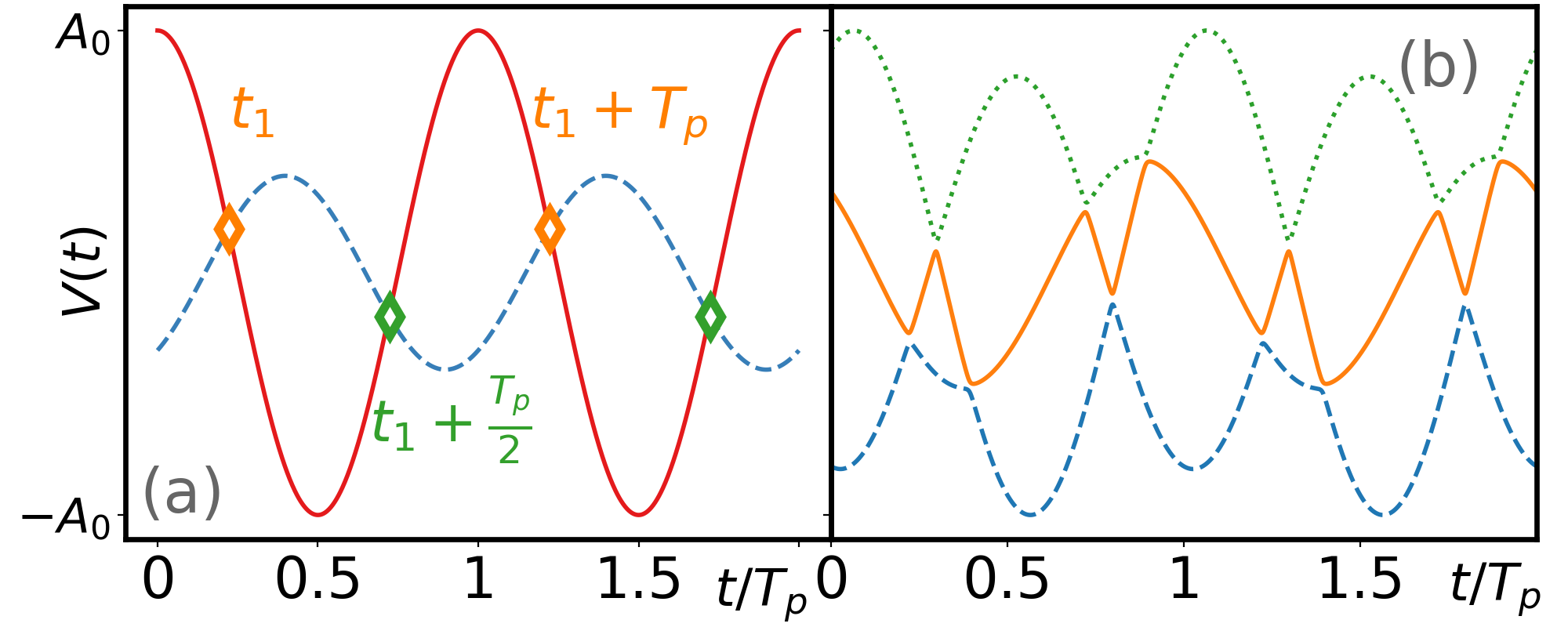
One dimension – Consider first the Holstein model on two sites. Although our goal is eventually to treat fully quantum phonons, consider first highly excited classical phonon states on each site, where the phonon has a large initial position and momentum (,) drawn from a thermal distribution, or else a quantum coherent state with the same (,). If the hopping is zero, the problem is exactly solvable. If the electron is on site , the electronic energy varies as from the electron-phonon coupling. If the electron is on site , the behavior is similar, with a different amplitude and phase as shown in Fig. 1(a). If nonzero electron hopping is added, one can treat the problem of a quantum electron in a time-dependent potential due to the phonons. In the adiabatic limit (small ), with smaller than a typical , the crossing of and becomes an avoided crossing. The electron that initially had most of its amplitude on site hops to site during the avoided crossing. If one assumes the functional form of and continues for all time, the electron hops from site to site every time interval [as shown in Fig. 1(a)], where is the phonon period, . Note that this is already a violation of the Boltzmann diffusion hypothesis, because the system does not lose memory of its initial state. Even in the long time limit, the electron probability is not spread equally on both sites, but rather retains memory of its initial state, alternating sites like clockwork, forever. Even in the fully quantum 2-site problem, solved numerically exactly with no approximations si , similar behavior is obtained for certain initial conditions. For example in the superposition of an even-parity and an odd-parity many-body eigenstate, the expectation of the excess density on site 1 oscillates like a cosine, forever.
If the other parameters are fixed, the typical on-site energies eventually become larger than the hopping as the temperature increases. Consider a one-dimensional array of sites with periodic boundary conditions at high temperature, with the electron initially on site with on-site energy . If the energy of the site on the right becomes equal to before the site on the left does, the first avoided crossing is between sites and , and the electron will hop to the right. Perhaps unexpectedly, if the electron’s first hop is to the right, all subsequent hops are also to the right. The reason is that if the electron hops right at time , the next avoided crossing that will allow it to hop right again occurs at a random time (depending on phonon amplitudes and phases) somewhere in the interval . But the next avoided crossing that would allow it to hop left is exactly at time , at the very end of the interval. The hop at the end of the interval occurs later than the one in the interior. Similarly, if the first hop is to the left, which happens half of the time, all subsequent hops will be to the left. This is illustrated in Fig. 1(b) in a periodic chain with 3 sites. From all three different initial states, the particle moves in constant direction. This behavior is completely different from diffusion. Instead of , it increases as . The average electron velocity is tied to the phonon frequency: it is a factor of order unity (= 4) times the lattice spacing divided by the phonon period. We call this approximation in which the electron hops to the neighboring site with the first avoided crossing the semiclassical approximation.
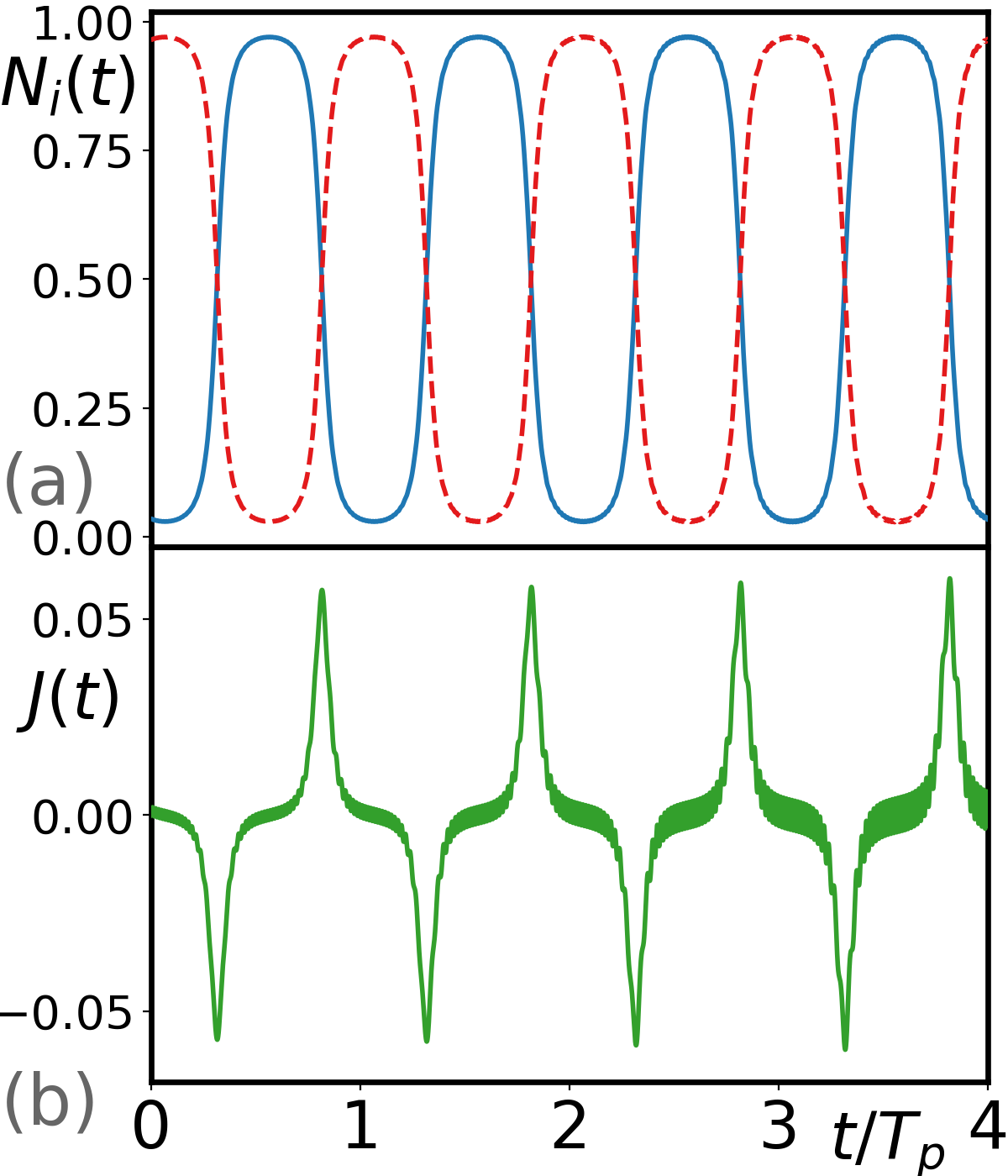
If a more accurate calculation, including fully quantum phonons and electron, confirms that the semiclassical approximation has some validity at high temperatures, this would require a change in the Boltzmann diffusion scenario. We will see below that more accurate calculations do provide some confirmation. First, as an intermediate step, we treat the itinerant particle as a quantum wavefunction and keep the phonons as local time-dependent potentials whose average amplitude increases with temperature as where is the mass of electron. In short, the last two terms in Eq. (1) are replaced by . We call this treatment the quantum electron (QE) approach. In this approximation, the initial wavefunction is (Floquet) periodically driven with period . The dynamics of the itinerant particle is simulated det by the time-dependent Schödinger equation, . Figures 2(a) and 2(b) show the time evolution of the particle and current densities in a two-site system. On each site, the particle density oscillates over time with period , with small components at higher frequencies. The current density on the link shows a narrow peak as the particle density switches from site to site during the avoided crossing. The results agree with the semiclassical approach, which states that the particle jumps between the two sites repeatedly and stays at each site for half a phonon period.
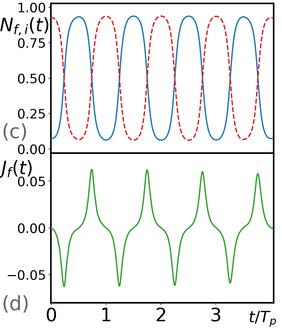
Finally, we consider the Holstein model of Eq. (1) without any approximation, so that both the phonons and the electron are treated quantum mechanically. The eigenstates and dynamics can be simulated accurately by the time-dependent Lanczos method Avella and Mancini (2013); Zhang et al. (2010); Lai and Chien (2016); Bonča et al. (1999); Kogoj et al. (2016); Hochbruck and Lubich (2006); Moler and Van Loan (2003). Here, the temperature and the coupling are two independent variables. Due to the unbounded Hilbert space of local phonons, the system size is restricted to be small and a cutoff on total phonon quanta is introduced. We call the numerically exact complete quantum mechanical treatment the fully quantum (FQ) approach. We construct the initial state of the quantum phonons by using phonon coherent states Shankar (1994),
| (2) |
where represents the temperature, and the wavefunction of the itinerant particle is taken to be an eigenstate (usually the ground state) of the Hamiltonian with effective local potentials determined from the initial phonon wavefunction si . Figures 2(c) and 2(d) present the time evolution of particle and current densities from this given initial state in a two-site system. The maximum particle density oscillates from site to site and the current density shows a narrow peak as the particle rapidly switches from site to site. In summary, for a two-site system, the itinerant particle stays at each site for half a phonon period before jumping to the other site in all three different approaches. This microscopic dynamics is not diffusive.
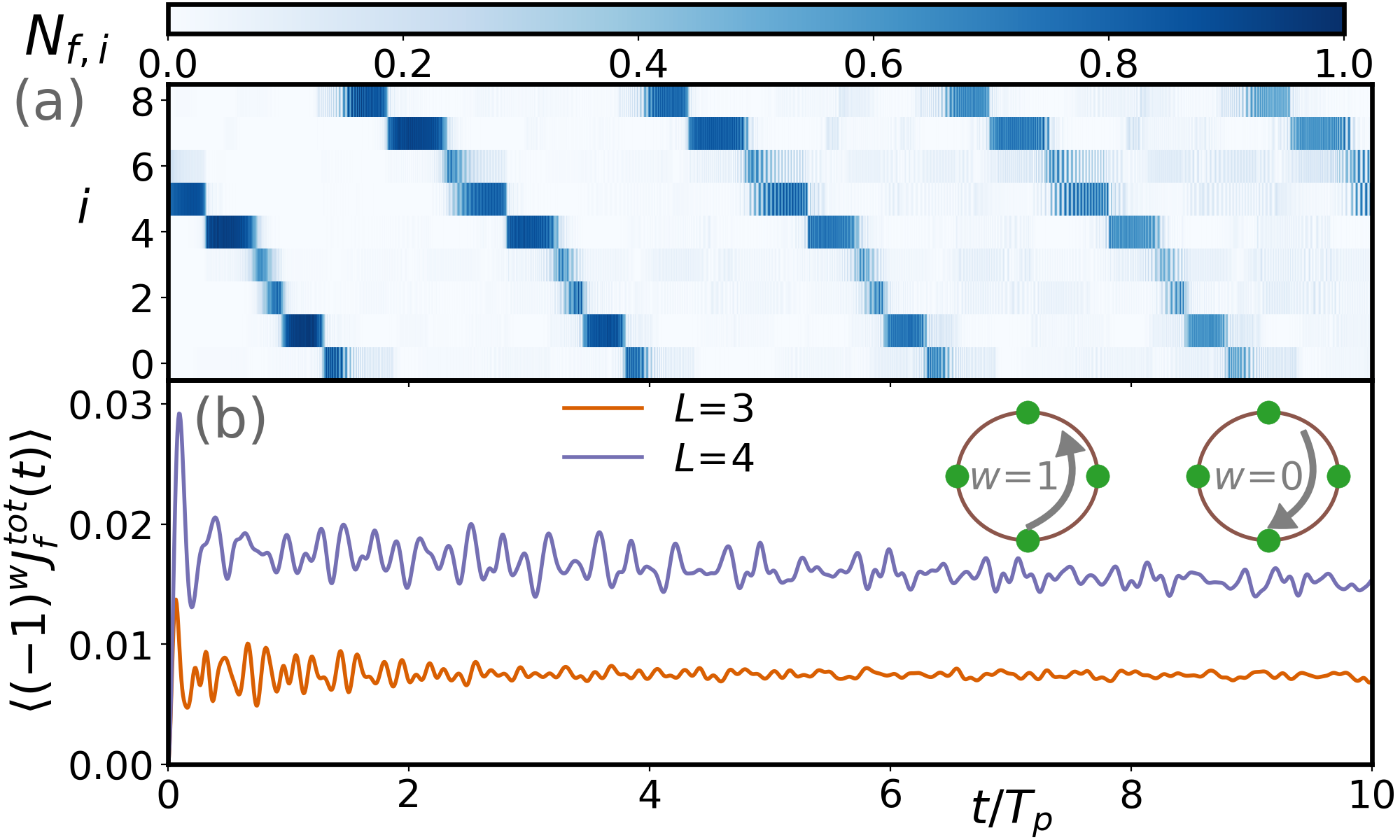
As discussed above, in a one dimensional periodic chain, the itinerant particle travels in a constant direction given by the initial conditions in the semiclassical approximation. Figure 3(a) shows one realization from the QE model that follows this prediction for a long time. In a FQ simulation shown in Fig. 3(b) starting from phonon coherent states, the total current retains its initial sign and does not decay to zero after ten phonon periods (about 36 hops), in the thermal ensemble average. This indicates that there is a non-zero circulating current in the periodic chain in either one of the directions: clockwise or counterclockwise. In a diffusion picture, this quantity would decay rapidly to zero as the particle has an equal chance to move right or left.
The simple semiclassical model assumes that the electron jumps at the first avoided crossing. This is an oversimplification, in that in a random ensemble, sometimes the second avoided crossing is only very slightly later, and it would be expected that part of the quantum amplitude moves in each direction. In contrast, in both the QE and FQ simulations, there is no assumption that the particle jumps at the first avoided crossing, nor that the particle starts from a single site. All phonon initial conditions are included in the ensemble average as the amplitudes are drawn from a thermal distribution and the phase chosen at random. Even in the more accurate QE and the exact FQ simulations, the persistence of the current and lack of diffusion first argued from the simple semiclassical model persist.
The particle is expected to follow the semiclassical prediction only in certain parameter regimes. First, Landau-Zener tunneling should be weak (the trajectory should usually not change color in Fig. 1b), which gives Landau (1932); Zener (1932); si
| (3) |
An implicit assumption of the semiclassical and QE models is that the amplitude and phase of the phonon oscillation is not affected when the electron hops on and off a site. This approximation is accurate if
| (4) |
This second condition is satisfied at higher temperatures that excite more phonon quanta, and at weaker elextron-phonon coupling . Both conditions are tested numerically and presented in the Supplemental Material si .
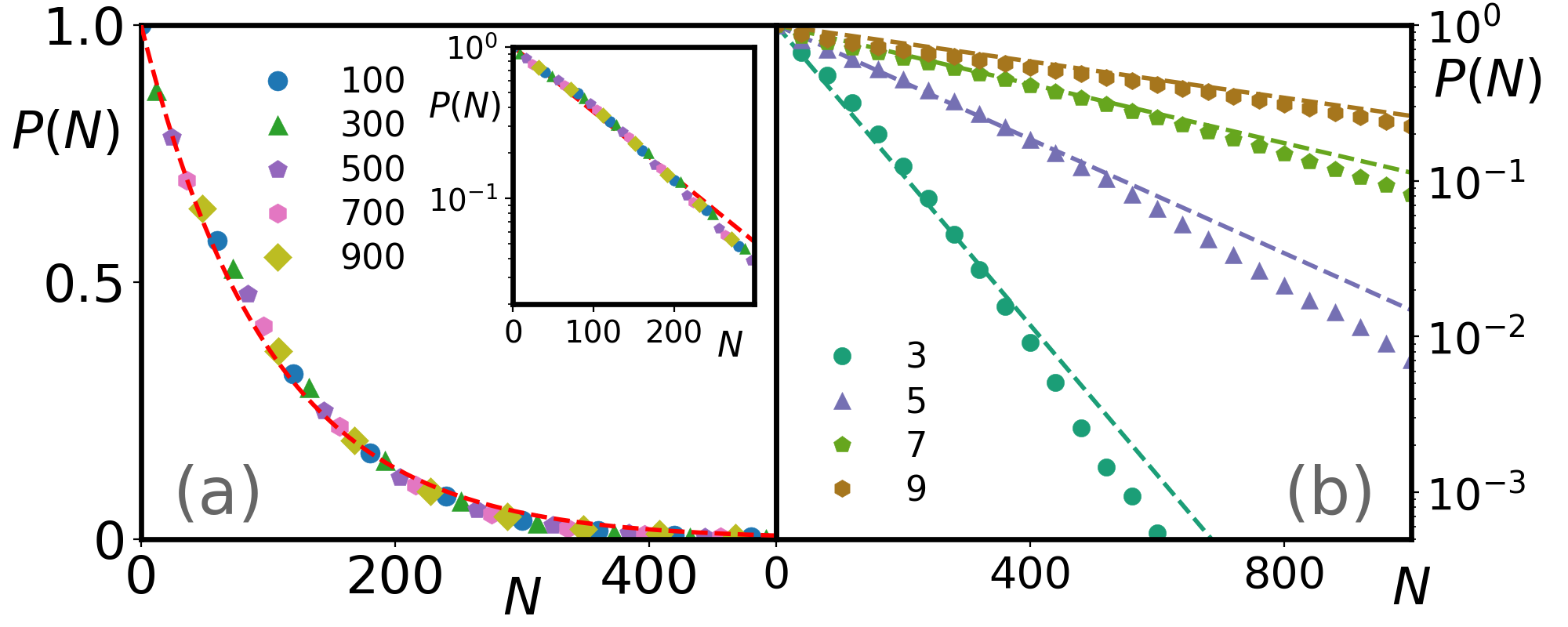
Ladders – In the one dimensional chain with periodic boundary conditions, the particle travels through the entire chain and back to its starting point in the semiclassical model. For a ladder system (), the particle need not visit all lattice sites, and a repeating closed trajectory on a square lattice can contain as few as 4 sites. In the semiclassical approximation, in any finite system, the particle always traces a closed trajectory that is repeated periodically in the future and past. Moreover, the particle will not trace the same bond in the same direction more than once before closing the trajectory. Thus, the maximum number of steps to close a trajectory is where the factor is counting both directions and is total number of bonds in the finite system. The above two statements are numerically verified in the semiclassical model, and simulations from the QE model draw similar conclusions and are presented in the Supplemental Material. In order to give a more quantitative analysis of the dynamics, the number of jumps in the closed trajectory, , is simulated for more than realizations of the initial conditions for the semiclassical model. We aim to answer whether the particle will have a finite trajectory, with probability 1, in the thermodynamic limit. Here, the probability of taking more than jumps to close a trajectory is used to quantify the behavior of the itinerant particle. Explicitly, we define
| (5) |
where is the probability of taking jumps to close the trajectory. First, by keeping number of rungs fixed and expanding the length of the chain , the results in Fig. 4(a) show that decays exponentially and follows the same scaling regarding different lengths. The results of increasing the number of rungs in Fig. 4(b) as the system approaches a two-dimensional (2D) square lattice show that the exponent decreases as increases.
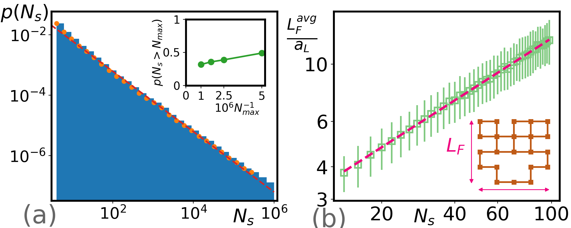
Square lattices – Next, we consider the dynamics on an infinite two dimensional square lattice with a cut-off maximum () of jumps in the semiclassical model. Unlike the ladder systems, the probability decays as power law as shown in Fig. 5(a), rather than exponentially. This power law decay indicates that the system is critical in 2D. The inset show the probability of having more than jumps as a function of . The finite size scaling extrapolation of appears to show that a finite fraction of the trajectories in 2D, approximately , are infinite and never close. The critical behavior suggests that the trajectory is fractal. Let be the edge length of the smallest square box that can enclose a given trajectory. Figure 5(b) shows that the relation between the average and the number of jumps between and . The average size of the square scales as with non-integer exponent , which indicates that the trajectory is fractal. The fractal geometry found here is qualitatively similar to the one in the integer quantum Hall effect Wang et al. (2015); Dean et al. (2013); Trugman (1989) where the particle travels in a random potential in a magnetic field.
Conclusions – The microscopic dynamics of an electron in the Holstein model of electron-phonon coupling at high temperatures is studied in two approximations, and in a numerically exact fully quantum approach. The results of these approaches agree with each other qualitatively, at least for intermediate times. Surprisingly, the dynamics are not diffusive. In a periodic one-dimensional chain, the electron will move in a single direction, return to its starting point, and loop repeatedly. On ladder systems, the particle travels in a closed loop, with long trajectories exponentially rare. On a 2D lattice, the system is critical. The trajectories are fractal, long trajectories have a power law probability, and a finite fraction of the trajectories are infinite (never close).
Acknowledgements.
The authors thank Eli Ben-Naim, Janez Bonc̆a, Peter Prelovs̆ek, and Daniel Trugman for fruitful discussions. This work was performed, in part, at the Center for Integrated Nanotechnologies, an Office of Science User Facility operated for the U.S. Department of Energy (DOE) Office of Science. Los Alamos National Laboratory (LANL), an affirmative action equal opportunity employer, is managed by Triad National Security, LLC for the U.S. Department of Energy’s NNSA, under contract 89233218CNA000001. This work was also supported by LANL LDRD. Computational resources were provided by the LANL Institutional Computing Program.References
- Holstein (1959) T. Holstein, Annals of Physics 8, 325 (1959), ISSN 0003-4916.
- Madelung and Taylor (1978) O. Madelung and B. Taylor, Introduction to Solid-State Theory, Springer Series in Solid-State Sciences (Springer-Verlag, 1978), ISBN 978-3-540-08516-4.
- Mishchenko et al. (2015) A. S. Mishchenko, N. Nagaosa, G. De Filippis, A. de Candia, and V. Cataudella, Phys. Rev. Lett. 114, 146401 (2015).
- (4) Please see supplemental information.
- (5) The initial state is choosen as the ground state of the Hamiltonian at time and the real time dynamics is solved by fourth-order Runge-Kutta with time step where the time unit is .
- Avella and Mancini (2013) A. Avella and F. Mancini, eds., Strongly Correlated Systems, Numerical Methods (Springer-Verlag, Berlin Heidelberg, 2013), ISBN 3-642-35106-9.
- Zhang et al. (2010) J. Zhang, Y. Tang, K. Lee, and M. Ouyang, Nature 466, 91 (2010).
- Lai and Chien (2016) C.-Y. Lai and C.-C. Chien, Sci. Rep. 6, 37256 (2016).
- Bonča et al. (1999) J. Bonča, S. A. Trugman, and I. Batistić, Phys. Rev. B 60, 1633 (1999).
- Kogoj et al. (2016) J. Kogoj, L. Vidmar, M. Mierzejewski, S. A. Trugman, and J. Bonča, Phys. Rev. B 94, 014304 (2016).
- Hochbruck and Lubich (2006) M. Hochbruck and C. Lubich, SIAM J Numer Anal 34, 1911 (2006).
- Moler and Van Loan (2003) C. Moler and C. Van Loan, SIAM Rev 45, 3 (2003).
- Shankar (1994) R. Shankar, Principles of Quantum Mechanics (Springer, 1994).
- Landau (1932) L. Landau, Sov. Fiz. Zhurnal 2, 46 (1932).
- Zener (1932) C. Zener, Proceedings of the Royal Society of London. Series A, Containing Papers of a Mathematical and Physical Character 137, 696 (1932).
- Wang et al. (2015) L. Wang, Y. Gao, B. Wen, Z. Han, T. Taniguchi, K. Watanabe, M. Koshino, J. Hone, and C. R. Dean, Science 350, 1231 (2015), ISSN 0036-8075, 1095-9203.
- Dean et al. (2013) C. R. Dean, L. Wang, P. Maher, C. Forsythe, F. Ghahari, Y. Gao, J. Katoch, M. Ishigami, P. Moon, M. Koshino, et al., Nature 497, 598 (2013), ISSN 1476-4687.
- Trugman (1989) S. A. Trugman, Phys. Rev. Lett. 62, 579 (1989).