AABO: Adaptive Anchor Box Optimization for Object Detection via Bayesian Sub-sampling
Abstract
Corresponding Author: [email protected]Most state-of-the-art object detection systems follow an anchor-based diagram. Anchor boxes are densely proposed over the images and the network is trained to predict the boxes position offset as well as the classification confidence. Existing systems pre-define anchor box shapes and sizes and ad-hoc heuristic adjustments are used to define the anchor configurations. However, this might be sub-optimal or even wrong when a new dataset or a new model is adopted. In this paper, we study the problem of automatically optimizing anchor boxes for object detection. We first demonstrate that the number of anchors, anchor scales and ratios are crucial factors for a reliable object detection system. By carefully analyzing the existing bounding box patterns on the feature hierarchy, we design a flexible and tight hyper-parameter space for anchor configurations. Then we propose a novel hyper-parameter optimization method named AABO to determine more appropriate anchor boxes for a certain dataset, in which Bayesian Optimization and sub-sampling method are combined to achieve precise and efficient anchor configuration optimization. Experiments demonstrate the effectiveness of our proposed method on different detectors and datasets, e.g. achieving around 2.4% mAP improvement on COCO, 1.6% on ADE and 1.5% on VG, and the optimal anchors can bring 1.4% 2.4% mAP improvement on SOTA detectors by only optimizing anchor configurations, e.g. boosting Mask RCNN from 40.3% to 42.3%, and HTC detector from 46.8% to 48.2%.
Keywords:
Object detection, Hyper-parameter optimization, Bayesian optimization, Sub-sampling1 Introduction
Object detection is a fundamental and core problem in many computer vision tasks and is widely applied on autonomous vehicles [4], surveillance camera [22], facial recognition [2], to name a few. Object detection aims to recognize the location of objects and predict the associated class labels in an image. Recently, significant progress has been made on object detection tasks using deep convolution neural network [21, 26, 28, 18]. In many of those deep learning based detection techniques, anchor boxes (or default boxes) are the fundamental components, serving as initial suggestions of object’s bounding boxes. Specifically, a large set of densely distributed anchors with pre-defined scales and aspect ratios are sampled uniformly over the feature maps, then both shape offsets and position offsets relative to the anchors, as well as classification confidence, are predicted using a neural network.
While anchor configurations are rather critical hyper-parameters of the neural network, the design of anchors always follows straight-forward strategies like handcrafting or using statistical methods such as clustering. Taking some widely used detection frameworks for instance, Faster R-CNN [28] uses pre-defined anchor shapes with 3 scales () and 3 aspect ratios (, , ), and YOLOv2 [27] models anchor shapes by performing k-means clustering on the ground-truth of bounding boxes. And when the detectors are extended to a new certain problem, anchor configurations must be manually modified to adapt the property and distribution of this new domain, which is difficult and inefficient, and could be sub-optimal for the detectors.
While it is irrational to determine hyper-parameters manually, recent years have seen great development in hyper-parameter optimization (HPO) problems and a great quantity of HPO methods are proposed. The most efficient methods include Bayesian Optimization (BO) and bandit-based policies. BO iterates over the following three steps: a) Select the point that maximizes the acquisition function. b) Evaluate the objective function. c) Add the new observation to the data and refit the model, which provides an efficacious method to select promising hyper-parameters with sufficient resources. Different from BO, Bandit-based policies are proposed to efficiently measure the performance of hyper-parameters. Among them, Hyperband [17] (HB) makes use of cheap-to-evaluate approximations of the acquisition function on smaller budgets, which calls SuccessiveHalving [14] as inner loop to identify the best out of randomly-sampled configurations. Bayesian Optimization and Hyperband (BOHB) introduced in [10] combined these two methods to deal with HPO problems in a huge search space, and it is regarded as a very advanced HPO method. However, BOHB is less applicable to our anchor optimization problems, because the appropriate anchors for small objects are always hard to converge, then the optimal anchor configurations could be early-stopped and discarded by SuccesiveHalving.
In this paper, we propose an adaptive anchor box optimization method named AABO to automatically discover optimal anchor configurations, which can fully exploit the potential of the modern object detectors. Specifically, we illustrate that anchor configurations such as the number of anchors, anchor scales and aspect ratios are crucial factors for a reliable object detector, and demonstrate that appropriate anchor boxes can improve the performance of object detection systems. Then we prove that anchor shapes and distributions vary distinctly across different feature maps, so it is irrational to share identical anchor settings through all those feature maps. So we design a tight and adaptive search space for feature map pyramids after meticulous analysis of the distribution and pattern of the bounding boxes in existing datasets, to make full use of the search resources. After optimizing the anchor search space, we propose a novel hyper-parameter optimization method combining the benefits of both Bayesian Optimization and sub-sampling method. Compared with existing HPO methods, our proposed approach uses sub-sampling method to estimate acquisition function as accurately as possible, and gives opportunity to the configuration to be assigned with more budgets if it has chance to be the best configuration, which can ensure that the promising configurations will not be discarded too early. So our method can efficiently determine more appropriate anchor boxes for a certain dataset using limited computation resources, and achieves better performance than previous HPO methods such as random search and BOHB.
We conduct extensive experiments to demonstrate the effectiveness of our proposed approach. Significant improvements over the default anchor configurations are observed on multiple benchmarks. In particular, AABO achieves 2.4% mAP improvement on COCO, 1.6% on ADE and 1.5% on VG by only changing the anchor configurations, and consistently improves the performance of SOTA detectors by 1.4% 2.4%, e.g. boosts Mask RCNN [11] from 40.3% to 42.3% and HTC [7] from 46.8% to 48.2% in terms of mAP.
2 Related Work
2.0.1 Anchor-Based Object Detection.
Modern object detection pipelines based on CNN can be categorized into two groups: One-stage methods such as SSD [21] and YOLOv2 [27], and two-stage methods such as Faster R-CNN [28] and R-FCN [9]. Most of those methods make use of a great deal of densely distributed anchor boxes. In brief, those modern detectors regard anchor boxes as initial references to the bounding boxes of objects in an image. The anchor shapes in those methods are typically determined by manual selection [21, 28, 9] or naive clustering methods [27]. Different from the traditional methods, there are several works focusing on utilizing anchors more effectively and efficiently [32, 34]. MetaAnchor [32] introduces meta-learning to anchor generation, which models anchors using an extra neural network and computes anchors from customized priors. However, the network becomes more complicated. Zhong et al. [34] tries to learn the anchor shapes during training via a gradient-based method while the continuous relaxation may be not appropriate.
2.0.2 Hyper-paramter Optimization.
Although deep learning has achieved great successes in a wide range, the performance of deep learning models depends strongly on the correct setting of many internal hyper-parameters, which calls for an effective and practical solution to the hyper-parameter optimization (HPO) problems. Bayesian Optimization (BO) has been successfully applied to many HPO works. For example, [30] obtained state-of-the-art performance on CIFAR-10 using BO to search out the optimal hyper-parameters for convolution neural networks. And [23] won 3 datasets in the 2016 AutoML challenge by automatically finding the proper architecture and hyper-parameters via BO methods. While BO approach can converge to the best configurations theoretically, it requires an awful lot of resources and is typically computational expensive. Compared to Bayesian method, there exist bandit-based configuration evaluation approaches based on random search such as Hyperband [17], which could dynamically allocate resources and use SuccessiveHalving [14] to stop poorly performing configurations. Recently, some works combining Bayesian Optimization with Hyperband are proposed like BOHB [10], which can obtain strong performance as well as fast convergence to optimal configurations. Other non-parametric methods that have been proposed include -greedy and Boltzmann exploration [31]. [5] proposed an efficient non-parametric solution and proved optimal efficiency of the policy which would be extended in our work. However, there exist some problems in those advanced HPO methods such as expensive computation in BO and early-stop in BOHB.
3 The Proposed Approach
3.1 Preliminary Analysis
As mentioned before, mainstream detectors, including one-stage and two-stage detectors, rely on anchor boxes to provide initial guess of the object’s bounding box. And most detectors pre-define anchors and manually modify them when applied on new datasets. We believe that those manual methods can hardly find optimal anchor configurations and sub-optimal anchors will prevent the detectors from obtaining the optimal performance. To confirm this assumption, we construct two preliminary experiments.
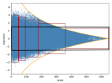
Default Anchors Are Not Optimal. We randomly sample 100 sets of different anchor settings, each with 3 scales and 3 ratios. Then we examine the performance of Faster-RCNN [28] under those anchor configurations. The results are shown in Figure 1.


It’s obvious that compared with default anchor setting (3 anchor scales: and 3 aspect ratios: , , and ), randomly-sampled anchor settings could significantly influence the performance of the detector, which clearly demonstrates that the default anchor settings may be less appropriate and the optimization of anchor boxes is necessary.
Anchors Influence More Than RPN Structure. Feature Pyramid Networks [18] (FPN) introduces a top-down pathway and lateral connections to enhance the semantic representation of low-level features and is a widely used feature fusion scheme in modern detectors. In this section, we use BOHB [10] to search RPN head architecture in FPN as well as anchor settings simultaneously. The search space of RPN Head is illustrated in Figure 1. The searched configurations, including RPN head architecture and anchor settings, are reported in the appendix. Then we analyze the respective contributions of RPN head architecture and anchor settings, and the results are shown in Table 1. Here, mean Average Precision is used to measure the performance and is denoted by mAP.
| Performance | mAP | AP50 | AP75 | APS | APM | APL |
|---|---|---|---|---|---|---|
| Baseline | 36.4 | 58.2 | 39.1 | 21.3 | 40.1 | 46.5 |
| Only Anchor | 37.1+0.7 | 58.4 | 40.0 | 20.6 | 40.8 | 49.5 |
| Only Architecture | 36.3-0.1 | 58.3 | 38.9 | 21.6 | 40.2 | 46.1 |
| Anchor+Architecture | 37.2+0.8 | 58.7 | 40.2 | 20.9 | 41.3 | 49.1 |
The results in Table 1 illustrate that searching for proper anchor configurations could bring more performance improvement than searching for RPN head architecture to a certain extent.
Thus, the conclusion comes clearly that anchor settings affect detectors substantially, and proper anchor settings could bring considerable improvement than doing neural architecture search (NAS) on the architecture of RPN head. Those conclusions indicate that the optimization of anchor configurations is essential and rewarding, which motivates us to view anchor configurations as hyper-parameters and propose a better HPO method for our anchor optimization case.
3.2 Search Space Optimization for Anchors
Since we have decided to search appropriate anchor configurations to increase the performance of detectors over a certain dataset, one critical problem is how to design the search space. In the preliminary analysis, we construct two experiments whose search space is roughly determined regardless of the distribution of bounding boxes. In this section, we will design a much tighter search space by analyzing the distribution characteristics of object’s bounding boxes.
For a certain detection task, we find that anchor distribution satisfies some properties and patterns as follows.
Upper and Lower Limits of the Anchors. Note that the anchor scale and anchor ratio are calculated from the and of the anchor, which are not independent. Besides, we discover that both anchor and are limited within fixed values, denoted by and . Then the anchor ratio and scale must satisfy constraints as follows:
| (1) |
From the formulas above, we calculate the upper bound and lower bound of the ratio for the anchor boxes:
| (2) |
Figure 2 shows an instance of the distribution of bounding boxes (the blue points) as well as the upper and lower bounds of anchors (the yellow curves) in COCO [20] dataset. And the region inside the black rectangle is the previous search space using in preliminary experiments. We can observe that there exists an area which is beyond the upper and lower bounds so that bounding boxes won’t appear, while the search algorithm will still sample anchors here. So it’s necessary to limit the search space within the upper and lower bounds.
Adaptive Feature-Map-Wised Search Space. We then study the distribution of anchor boxes in different feature maps of Feature Pyramid Networks (FPN)[18] and discover that the numbers, scales and ratios of anchor boxes vary a lot across different feature maps, shown in the right subgraph of Figure 2. There are more and bigger bounding boxes in lower feature maps whose receptive fields are smaller, less and tinier bounding boxes in higher feature maps whose respective fields are wider.
As a result, we design an adaptive search space for FPN [18] as shown in the left subgraph of Figure 2. The regions within 5 red rectangles and the anchor distribution bounds represent the search space for each feature map in FPN. As feature maps become higher and smaller, the numbers of anchor boxes are less, as well as the anchor scales and ratios are limited to a narrower range.


Compared with the initial naive search space, we define a tighter and more adaptive search space for FPN [18], as shown in Figure 3. Actually, the new feature-map-wised search space is much bigger than the previous one, which makes it possible to select more flexible anchors and cover more diverse objects with different sizes and shapes. Besides, the tightness of the search space can help HPO algorithms concentrate limited resources on more meaningful areas and avoid wasting resources in sparsely distributed regions of anchors.
3.3 Bayesian Anchor Optimization via Sub-sampling
As described before, we regard anchor configurations as hyper-parameters and try to use HPO method to choose optimal anchor settings automatically. However, existing HPO methods are not suitable for solving our problems. For random search or grid search, it’s unlikely to find a good solution because the search space is too big for those methods. For Hyperband or BOHB, the proper configurations for the small objects could be discarded very early since the anchors of small objects are always slowly-converged. So we propose a novel method which combines Bayesian Optimization and sub-sampling method, to search out the optimal configurations as quickly as possible.
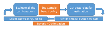
Specifically, our proposed approach makes use of BO to select potential configurations, which estimates the acquisition function based on the configurations already evaluated, and then maximizes the acquisition fuction to identify promising new configurations. Meanwhile, sub-sampling method is employed to determine which configurations should be allocated more budgets, and explore more configurations in the search space. Figure 4 illustrates the process of our proposed method. In conclusion, our approach can achieve good performance as well as better speed, and take full advantage of models built on previous budgets.
Bayesian Optimization. Bayesian Optimization (BO) is a sequential design strategy for parameter optimization of black-box functions. In hyper-parameter optimization problems, the validation performance of machine learning algorithms is regarded as a function of hyper-parameters , and hyper-parameter optimization problem aims to determine the optimal . In most machine learning problems, is unobservable, so Bayesian Optimization approach treats it as a random function with a prior over it. Then some data points are sampled and BO updates the prior and models the function based on those gathering data points and evaluations. Then new data points are selected and observed to refit the model function.
In our approach, we use Tree Parzen Estimator (TPE) [1] which uses a kernel density estimator to model the probability density functions and instead of modeling function directly, where and , as seen in BOHB [10]. Note that there exists a serious problem that the theory of Hyperband only guarantees to return the best which has the smallest among all these configurations, while the quality of other configurations may be very poor. Consequently, larger responses lead to an inaccurate estimation of , which plays an important role in TPE. Thus, we need to propose a policy that has a better sequence of responses to solve this problem.
Sub-Sample Method. To better explain the sub-sampling method used in our proposed approach, we first introduce the standard multi-armed bandit problem with arms in this section. Recall the traditional setup for the classic multi-armed bandit problem. Let be a given set of arms. Consider a sequential procedure based on past observations for selecting an arm to pull. Let be the number of observations from the arm , and is the number of total observations. Observations , are also called rewards from the arm . In each arm, rewards are assumed to be independent and identically distributed with expectation given by and . For simplicity, assume without loss of generality that the best arm is unique which is also assumed in [25] and [5].
A policy is a sequence of random variables denoting that at each time , the arm is selected to pull. Note that depends only on previous observations. The objective of a good policy is to minimize the regret
| (3) |
Note that for a data-driven policy , the regret monotonically increases with respect to . Hence, minimizing the growth rate of becomes an important criterion which will be considered later.
Then we introduce an efficient nonparametric solution to the multi-armed bandit problem. First, we revisit the Sub-sample Mean Comparisons (SMC) introduced in [5] for the HPO case. The set of configurations minimum budget and parameter are inputs. Output is the sequence of the configurations to be evaluated in order.
First, it is defined that the -th configuration is “better” than the -th configuration, if one of the following conditions holds:
-
1.
and .
-
2.
and , for some , where .
In SMC, let denotes the round number. In the first round, all configurations are evaluated since there is no information about them. In round , we define the leader of configurations which has been evaluated with the most budgets. And, the -th configuration will be evaluated with one more budget , if it is “better” than the leader. Otherwise, if there is no configuration “better” than the leader, the leader will be evaluated again. Hence, in each round, there are at most configurations and at least one configuration to be evaluated. Let be the total number of evaluations at the beginning of round , and be the corresponding number from the -th configuration. Then, we have .
The Sub-sample Mean Comparisons(SMC) is shown in Algorithm 1. In SMC, the parameter is a non-negative monotone increasing threshold for SMC satisfied that and as . In [5], they set for efficiency of SMC.
Note that when the round ends, the number of evaluations usually doesn’t equal to exactly, i.e., . For this case, configurations are randomly chosen from the configurations selected by SMC in the -th round. A main advantage of SMC is that unlike the UCB-based procedures, underlying probability distributions need not be specified. Still, it remains asymptotic optimal efficiency. The detailed discussion about theoretical results refers to [13].
4 Experiments
4.1 Datasets, Metrics and Implementation Details
We conduct experiments to evaluate the performance of our proposed method AABO on three object detection datasets: COCO 2017 [20], Visual Genome(VG) [16], and ADE [35]. COCO is a common object detection dataset with 80 object classes, containing 118K training images (train), 5K validation images (val) and 20K unannotated testing images (test-dev). VG and ADE are two large-scale object detection benchmarks with thousands of object classes. For COCO, we use the train split for training and val split for testing. For VG, we use release v1.4 and synsets [29] instead of raw names of the categories due to inconsistent annotations. Specifically, we consider two sets containing different target classes: VG1000 and VG3000, with 1000 most frequent classes and 3000 most frequent classes respectively. In both VG1000 and VG3000, we use 88K images for training, 5K images for testing, following [8, 15]. For ADE, we consider 445 classes, use 20K images for training and 1K images for testing, following [8, 15]. Besides, the ground-truths of ADE are given as segmentation masks, so we first convert them to bounding boxes for all instances before training.
As for evaluation, the results of the detection tasks are estimated with standard COCO metrics, including mean Average Precision (mAP) across IoU thresholds from 0.5 to 0.95 with an interval of 0.05 and AP50, AP75, as well as APS, APM and APL, which respectively concentrate on objects of small size (), medium size ( ) and large size ().
During anchor configurations searching, we sample anchor configurations and train Faster-RCNN [28] (combined with FPN [18]) using the sampled anchor configurations, then compare the performance of these models (regrading mAP as evaluation metrics) to reserve better anchor configurations and stop the poorer ones, following the method we proposed before. The search space is feature-map-wised as introduced. All the experiments are conducted on 4 servers with 8 Tesla V100 GPUs, using the Pytorch framework [24, 6]. ResNet-50 [12] pre-trained on ImageNet [29] is used as the shared backbone networks. We use SGD (momentum = 0.9) with batch size of 64 and train 12 epochs in total with an initial learning rate of 0.02, and decay the learning rate by 0.1 twice during training.
4.2 Anchor Optimization Results
We first evaluate the effectiveness of AABO over 3 large-scale detection datasets: COCO [20], VG [16] (including VG1000 and VG3000) and ADE [35]. We use Faster-RCNN [28] combined with FPN [18] as our detector, and the baseline model is FPN with default anchor configurations. The results are shown in Table 2 and the optimal anchors searched out by AABO are reported in the appendix.
| Dataset | Method | mAP | AP50 | AP75 | APS | APM | APL |
|---|---|---|---|---|---|---|---|
| COCO | Faster-RCNN w FPN | 36.4 | 58.2 | 39.1 | 21.3 | 40.1 | 46.5 |
| Search via AABO | 38.8+2.4 | 60.7+2.5 | 41.6+2.5 | 23.7+2.4 | 42.5+2.4 | 51.5+5.0 | |
| VG1000 | Faster-RCNN w FPN | 6.5 | 12.0 | 6.4 | 3.7 | 7.2 | 9.5 |
| Search via AABO | 8.0+1.5 | 13.2+1.2 | 8.2+1.8 | 4.2+0.5 | 8.3+1.1 | 12.0+2.5 | |
| VG3000 | Faster-RCNN w FPN | 3.7 | 6.5 | 3.6 | 2.3 | 4.9 | 6.8 |
| Search via AABO | 4.2+0.5 | 6.9+0.4 | 4.6+1.0 | 3.0+0.7 | 5.8+0.9 | 7.9+1.1 | |
| ADE | Faster-RCNN w FPN | 10.3 | 19.1 | 10.0 | 6.1 | 11.2 | 16.0 |
| Search via AABO | 11.9+1.6 | 20.7+1.6 | 11.9+1.9 | 7.4+1.3 | 12.2+1.0 | 17.5+1.5 |
It’s obvious that AABO outperforms Faster-RCNN with default anchor settings among all the 3 datasets. Specifically, AABO improves mAP by 2.4% on COCO, 1.5% on VG1000, 0.5% on VG3000, and 1.6% on ADE. The results illustrate that the pre-defined anchor used in common-used detectors are not optimal. Treat anchor configurations as hyper-parameters and optimize them using AABO can assist to determine better anchor settings and improve the performance of the detectors without increasing the complexity of the network.
Note that the searched anchors increase all the AP metrics, and the improvements on APL are always more significant than APS and APM : AABO boosts APL by 5% on COCO, 2.5% on VG1000, 1.1% on VG3000, and 1.5% on ADE. These results indicate that anchor configurations determined by AABO concentrate better on all objects, especially on the larger ones. It can also be found that AABO is especially useful for the large-scale object detection dataset such as VG3000. We conjecture that this is because the searched anchors can better capture the various sizes and shapes of objects in a large number of categories.
4.3 Benefit of the Optimal Anchor Settings on SOTA Methods
After searching out optimal anchor configurations via AABO, we apply them on several other backbones and detectors to study the generalization property of the anchor settings. For backbone, we change ResNet-50 [12] to ResNet-101 [12] and ResNeXt-101 [33], with detector (FPN) and other conditions constant. For detectors, we apply our searched anchor settings on several state-of-the-art detectors: a) Mask RCNN [11], b) RetinaNet [19], which is a one-stage detector, c) DCNv2 [36], and d) Hybrid Task Cascade (HTC) [7], with different backbones: ResNet-101 and ResNeXt-101. All the experiments are conducted on COCO.
The results are reported in Table 3. We can observe that the optimal anchors can consistently boost the performance of SOTA detectors, whether one-stage methods or two-stage methods. Concretely, the optimal anchors bring 2.1% mAP improvement on FPN with ResNet-101, 1.9% on FPN with ResNeXt-101, 2.0% on Mask RCNN, 1.4% on RetinaNet, 2.4% on DCNv2, and 1.4% improvement on HTC. The results demonstrate that our optimal anchors can be widely applicable across different network backbones and SOTA detection algorithms, including both one-stage and two-stage detectors. We also evaluate these optimized SOTA detectors on COCO test-dev, and the results are reported in the appendix. The performance improvements on val split and test-dev are consistent.
| Model | mAP | AP50 | AP75 | APS | APM | APL | |
|---|---|---|---|---|---|---|---|
| FPN[18] w r101 | Default | 38.4 | 60.1 | 41.7 | 21.6 | 42.7 | 50.1 |
| Searched | 40.5+2.1 | 61.8 | 43.3 | 23.4 | 43.6 | 51.3 | |
| FPN[18] w x101 | Default | 40.1 | 62.0 | 43.8 | 24.0 | 44.8 | 51.7 |
| Searched | 42.0+1.9 | 63.9 | 65.1 | 25.2 | 46.3 | 54.4 | |
| Mask RCNN[11] w r101 | Default | 40.3 | 61.5 | 44.1 | 22.2 | 44.8 | 52.9 |
| Searched | 42.3+2.0 | 63.6 | 46.3 | 26.1 | 46.3 | 55.3 | |
| RetinaNet[19] w r101 | Default | 38.1 | 58.1 | 40.6 | 20.2 | 41.8 | 50.8 |
| Searched | 39.5+1.4 | 60.2 | 41.9 | 21.7 | 42.7 | 53.7 | |
| DCNv2[36] w x101 | Default | 43.4 | 61.3 | 47.0 | 24.3 | 46.7 | 58.0 |
| Searched | 45.8+2.4 | 67.5 | 49.7 | 28.9 | 49.4 | 60.9 | |
| HTC[7] w x101 | Default | 46.8 | 66.2 | 51.2 | 28.0 | 50.6 | 62.0 |
| Searched | 48.2+1.4 | 67.3 | 52.2 | 28.6 | 51.9 | 62.7 | |
4.4 Comparison with Other Optimization Methods
Comparison with other anchor initialization methods. In this section, we compare AABO with several existing anchor initialization methods: a) Pre-define anchor settings, which is used in most modern detectors. b) Use k-means to obtain clusters and treat them as default anchors, which is used in YOLOv2 [27]. c) Use random search to determine anchors. d) Use AABO combined with Hyperband [17] to determine anchors. e) Use AABO (combined with sub-sampling) to determine anchors. Among all these methods, the latter three use HPO methods to select anchor boxes automatically, while a) and b) use naive methods like handcrafting and k-means. The results are recorded in Table 4.
Among all these anchor initialization methods, our proposed approach can boost the performance most significantly, bring 2.4% improvement than using default anchors, while the improvements of other methods including statistical methods and previous HPO methods are less remarkable. The results illustrate that the widely used anchor initialization approaches might be sub-optimal, while AABO can fully utilize the ability of advanced detection systems.
| Methods to Determine Anchor | mAP | AP50 | AP75 | APS | APM | APL | |
|---|---|---|---|---|---|---|---|
| Manual Methods | Pre-defined | 36.4 | 58.2 | 39.1 | 21.3 | 40.1 | 46.5 |
| Statistical Methods | K-Means | 37.0+0.6 | 58.9 | 39.8 | 21.9 | 40.5 | 48.5 |
| HPO | Random Search | 11.5-24.9 | 19.1 | 8.2 | 4.5 | 10.1 | 13.6 |
| AABO w HB | 38.2+1.8 | 59.3 | 40.7 | 22.6 | 42.1 | 50.1 | |
| AABO w SS | 38.8+2.4 | 60.7 | 41.6 | 23.7 | 42.5 | 51.5 | |
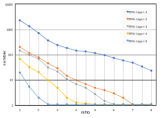
Comparison with other HPO methods. As Table 5 shows, our proposed method could find better anchor configurations in fewer trials and can improve the performance of the detector significantly: With single search space, AABO combined with HB and SS boosts the mAP of FPN [18] from 36.4% to 37.8% and 38.3% respectively, while random search only boosts 36.4% to 37.2%. With feature-map-wised search space, AABO combined with HB and SS can obtain 38.2% and 38.8% mAP respectively, while random search fails to converge due to the huge and flexible search space. The results illustrate the effectiveness and the high efficiency of our proposed approach.
| Search Space | Search | mAP of | number of searched |
| Method | optimal anchor | parameters | |
| Single | Random | 37.2 | 100 |
| AABO w HB | 37.8+0.6 | 64 | |
| AABO w SS | 38.3+1.1 | 64 | |
| Feature-Map-Wised | Random | 11.5 | 100 |
| AABO w HB | 38.2+26.7 | 64 | |
| AABO w SS | 38.8+27.3 | 64 |
Comparison with other anchor optimization methods. We also compare AABO with some previous anchor optimization methods like [34] and MetaAnchor [32]. As shown in Table 6, all these methods can boost the performance of detectors, while our method brings 2.4% mAP improvement on Faster-RCNN and 1.4% on RetinaNet, and the other two methods only bring 1.0% improvement, which demonstrates the superiority of our proposed AABO.
| Methods | YOLOv2 | RetinaNet | Faster-RCNN | RetinaNet |
|---|---|---|---|---|
| w Zhong’s Method [34] | w MetaAnchor [32] | w AABO | w AABO | |
| mAP of Baseline | 23.5 | 36.9 | 36.4 | 38.1 |
| mAP after Optimization | 24.5+1.0 | 37.9+1.0 | 38.8+2.4 | 39.5+1.4 |
4.5 Ablation Study
In this section, we study the effects of all the components used in AABO: a) Treat anchor settings as hyper-parameters, then use HPO methods to search them automatically. b) Use Bayesian Optimization method. c) Use sub-sampling method to determine the reserved anchors. d) Feature-map-wised search space.
As shown in Table 7, using HPO methods such as random search to optimize anchors can bring 0.8% performance improvement, which indicates the default anchors are sub-optimal. Using single search space (not feature-map-wised), AABO combined with HB brings 1.4% mAP improvement, and AABO combined with SS brings 1.9% mAP improvement, which demonstrates the advantage of BO and accurate estimation of acquisition function. Besides, our tight and adaptive feature-map-wised search space can give a guarantee to search out better anchors with limited computation resources, and brings about 0.5% mAP improvement as well. Our method AABO can increase mAP by 2.4% overall.
| Model | Search | BO | SS | Feature-map-wised | mAP | AP50 | AP75 | APS | APM | APL |
|---|---|---|---|---|---|---|---|---|---|---|
| Default | 36.4 | 58.2 | 39.1 | 21.3 | 40.1 | 46.5 | ||||
| Random Search | 37.2+0.8 | 58.8 | 39.9 | 21.7 | 40.6 | 48.1 | ||||
| 11.5-24.9 | 19.1 | 8.2 | 4.5 | 10.1 | 13.6 | |||||
| AABO w HB | 37.8+1.4 | 58.9 | 40.4 | 22.7 | 41.3 | 49.9 | ||||
| 38.2+1.8 | 59.3 | 40.7 | 22.6 | 42.1 | 50.1 | |||||
| AABO w SS | 38.3+1.9 | 59.6 | 40.9 | 22.9 | 42.2 | 50.8 | ||||
| 38.8+2.4 | 60.7 | 41.6 | 23.7 | 42.5 | 51.5 |
5 Conclusion
In this work, we propose AABO, an adaptive anchor box optimization method for object detection via Bayesian sub-sampling, where optimal anchor configurations for a certain dataset and detector are determined automatically without manually adjustment. We demonstrate that AABO outperforms both hand-adjusted methods and HPO methods on popular SOTA detectors over multiple datasets, which indicates that anchor configurations play an important role in object detection frameworks and our proposed method could help exploit the potential of detectors in a more effective way.
References
- [1] Bergstra, J.S., Bardenet, R., Bengio, Y., Kégl, B.: Algorithms for hyper-parameter optimization. In: NIPS (2011)
- [2] Bhagavatula, C., Zhu, C., Luu, K., Savvides, M.: Faster than real-time facial alignment: A 3d spatial transformer network approach in unconstrained poses. In: ICCV (2017)
- [3] Cai, Z., Vasconcelos, N.: Cascade r-cnn: High quality object detection and instance segmentation. IEEE Transactions on Pattern Analysis and Machine Intelligence (2019)
- [4] Chabot, F., Chaouch, M., Rabarisoa, J., Teuliere, C., Chateau, T.: Deep manta: A coarse-to-fine many-task network for joint 2d and 3d vehicle analysis from monocular image. In: CVPR (2017)
- [5] Chan, H.P.: The multi-armed bandit problem: An efficient non-parametric solution. Annals of Statistics p. To appear (2019)
- [6] Chen, K., Pang, J., Wang, J., Xiong, Y., Li, X., Sun, S., Feng, W., Liu, Z., Shi, J., Ouyang, W., Loy, C.C., Lin, D.: mmdetection. https://github.com/open-mmlab/mmdetection (2018)
- [7] Chen, K., Pang, J., Wang, J., Xiong, Y., Li, X., Sun, S., Feng, W., Liu, Z., Shi, J., Ouyang, W., Loy, C.C., Lin, D.: Hybrid task cascade for instance segmentation. In: IEEE Conference on Computer Vision and Pattern Recognition (2019)
- [8] Chen, X., Li, L.J., Fei-Fei, L., Gupta, A.: Iterative visual reasoning beyond convolutions. In: CVPR (2018)
- [9] Dai, J., Li, Y., He, K., Sun, J.: R-fcn: Object detection via region-based fully convolutional networks. In: NIPS (2016)
- [10] Falkner, S., Klein, A., Hutter, F.: Bohb: Robust and efficient hyperparameter optimization at scale. arXiv preprint arXiv:1807.01774 (2018)
- [11] He, K., Gkioxari, G., Dollar, P., Girshick, R.: Mask r-cnn. In: 2017 IEEE International Conference on Computer Vision (ICCV) (2017)
- [12] He, K., Zhang, X., Ren, S., Sun, J.: Deep residual learning for image recognition. In: CVPR (2016)
- [13] Huang, Y., Li, Y., Li, Z., Zhang, Z.: An Asymptotically Optimal Multi-Armed Bandit Algorithm and Hyperparameter Optimization. arXiv e-prints arXiv:2007.05670 (2020)
- [14] Jamieson, K., Talwalkar, A.: Non-stochastic best arm identification and hyperparameter optimization. In: Artificial Intelligence and Statistics. pp. 240–248 (2016)
- [15] Jiang, C., Xu, H., Liang, X., Lin, L.: Hybrid knowledge routed modules for large-scale object detection. In: NIPS (2018)
- [16] Krishna, R., Zhu, Y., Groth, O., Johnson, J., Hata, K., Kravitz, J., Chen, S., Kalantidis, Y., Li, L.J., Shamma, D.A., Bernstein, M., Fei-Fei, L.: Visual genome: Connecting language and vision using crowdsourced dense image annotations. International Journal of Computer Vision (2016)
- [17] Li, L., Jamieson, K., Desalvo, G., Rostamizadeh, A., Talwalkar, A.: Hyperband: A novel bandit-based approach to hyperparameter optimization. Journal of Machine Learning Research 18, 1–52 (2016)
- [18] Lin, T.Y., Dollár, P., Girshick, R., He, K., Hariharan, B., Belongie, S.: Feature pyramid networks for object detection. In: CVPR (2017)
- [19] Lin, T.Y., Goyal, P., Girshick, R., He, K., Dollár, P.: Focal loss for dense object detection. In: ICCV. pp. 2980–2988 (2017)
- [20] Lin, T.Y., Maire, M., Belongie, S., Hays, J., Perona, P., Ramanan, D., Dollár, P., Zitnick, C.L.: Microsoft coco: Common objects in context. In: ECCV (2014)
- [21] Liu, W., Anguelov, D., Erhan, D., Szegedy, C., Reed, S., Fu, C.Y., Berg, A.C.: Ssd: Single shot multibox detector. In: ECCV (2016)
- [22] Luo, P., Tian, Y., Wang, X., Tang, X.: Switchable deep network for pedestrian detection. In: CVPR (2014)
- [23] Mendoza, H., Klein, A., Feurer, M., Springenberg, J.T., Hutter, F.: Towards automatically-tuned neural networks. In: Workshop on Automatic Machine Learning. pp. 58–65 (2016)
- [24] Paszke, A., Gross, S., Chintala, S., Chanan, G., Yang, E., DeVito, Z., Lin, Z., Desmaison, A., Antiga, L., Lerer, A.: Automatic differentiation in pytorch. In: NIPS Workshop (2017)
- [25] Perchet, V., Rigollet, P.: The multi-armed bandit problem with covariates. Annals of Statistics 41(2), 693–721 (2013)
- [26] Redmon, J., Divvala, S., Girshick, R., Farhadi, A.: You only look once: Unified, real-time object detection. In: CVPR (2016)
- [27] Redmon, J., Farhadi, A.: Yolo9000: better, faster, stronger. In: CVPR (2017)
- [28] Ren, S., He, K., Girshick, R., Sun, J.: Faster r-cnn: Towards real-time object detection with region proposal networks. In: NIPS (2015)
- [29] Russakovsky, O., Deng, J., Su, H., Krause, J., Satheesh, S., Ma, S., Huang, Z., Karpathy, A., Khosla, A., Bernstein, M., et al.: Imagenet large scale visual recognition challenge. IJCV 115(3), 211–252 (2015)
- [30] Snoek, J., Larochelle, H., Adams, R.P.: Practical bayesian optimization of machine learning algorithms. In: NIPS (2012)
- [31] Sutton, R.S., Barto, A.G.: Reinforcement learning: An introduction. MIT press (2018)
- [32] Tong, Y., Zhang, X., Zhang, W., Jian, S.: Metaanchor: Learning to detect objects with customized anchors (2018)
- [33] Xie, S., Girshick, R., Dollár, P., Tu, Z., He, K.: Aggregated residual transformations for deep neural networks. In: CVPR. pp. 1492–1500 (2017)
- [34] Zhong, Y., Wang, J., Peng, J., Zhang, L.: Anchor box optimization for object detection. arXiv preprint arXiv:1812.00469 (2018)
- [35] Zhou, B., Zhao, H., Puig, X., Fidler, S., Barriuso, A., Torralba, A.: Scene parsing through ade20k dataset. In: CVPR (2017)
- [36] Zhu, X., Hu, H., Lin, S., Dai, J.: Deformable convnets v2: More deformable, better results. arXiv preprint arXiv:1811.11168 (2018)
Appendix
Optimal FPN Hyper-parameters in Preliminary Analysis
In preliminary analysis, we search for better RPN head architecture in FPN [18] as well as anchor settings simultaneously, to compare the respective contributions of changing RPN head architecture and anchor settings. The optimal hyper-parameters are shown in Table 8. Since the search space for RPN head architecture and anchor settings are both relatively small, the performance increase is not very significant.
| Hyper-parameter | Conv Layers | Kernel Size | Dilation Size |
|---|---|---|---|
| Optimal Configuration | 2 | 5x5 | 1 |
| Hyper-parameter | Location of ReLU | Anchor Scales | Anchor Ratios |
| Optimal Configuration | Behind 5x5 Conv | 2.5, 5.7, 13.4 | 2:5, 1:2, 1, 2:1, 5:2 |
Optimal Anchor Configurations
In this section, we record the best configurations searched out by AABO and analyze the difference between the results of default Faster-RCNN [28] and optimized Faster-RCNN.
As we design an adaptive feature-map-wised search space for anchor optimization, anchor configurations distribute variously in different layers of FPN [18]. Table 9 shows the optimal anchor configurations in FPN for COCO [20] dataset. We can observe that anchor scales and anchor ratios are larger and more diverse in shallower layers of FPN, while anchors tend to be smaller and more square in deeper layers.
| FPN-Layer | Anchor Number | Anchor Scales | Anchor Ratios |
|---|---|---|---|
| Layer-1 | 9 | {5.2, 6.1, 3.4, 4.9, 5.8, 4.8, 14.6, 7.4, 10.3} | {6.0, 0.3, 0.5, 1.6, 1.7, 2.6, 0.5, 0.5, 0.6} |
| Layer-2 | 6 | {11.0, 7.6, 11.8, 4.7, 5.7, 3.8} | {0.2, 2.0, 2.3, 2.8, 1.0, 0.5} |
| Layer-3 | 7 | {10.5, 11.1, 8.5, 6.7, 12.4, 4.6, 3.5} | {0.4, 4.2, 2.2, 1.6, 2.3, 0.5, 1.1} |
| Layer-4 | 6 | {5.7, 8.5, 7.0, 11.2, 15.2, 15.5} | {0.3, 0.4, 0.8, 0.7, 2.9, 2.8} |
| Layer-5 | 5 | {5.0, 4.2, 14.0, 10.1, 7.8} | {1.1, 1.4, 0.8, 0.7, 2.5} |
Improvements on SOTA Detectors over COCO Test-Dev
After searching out optimal anchor configurations via AABO, we apply them on several SOTA detectors to study the generalization property of the anchor settings. In this section, we report the performance of these optimized detectors on COCO test-dev split. The results are shown in Table 10.
It can be seen that the optimal anchors can consistently boost the performance of SOTA detectors on both COCO val split and COCO test-dev. Actually, the mAP of the optimized detectors on test-dev is even higher than the mAP on val, which illustrates that the optimized anchor settings could bring consistent performance improvements on val split and test-dev.
| Model | Anchor Setting | Eval on | mAP |
|---|---|---|---|
| Mask RCNN[11] w r101 | Default | val | 40.3 |
| Searched via AABO | val | 42.3+2.0 | |
| Searched via AABO | test-dev | 42.6+2.3 | |
| DCNv2[36] w x101 | Default | val | 43.4 |
| Searched via AABO | val | 45.8+2.4 | |
| Searched via AABO | test-dev | 46.1+2.7 | |
| Cascade Mask RCNN[3] w x101 | Default | val | 44.3 |
| Searched via AABO | val | 46.8+2.5 | |
| Searched via AABO | test-dev | 47.2+2.9 | |
| HTC*[7] w x101 | Default | val | 47.5 |
| Searched via AABO | val | 50.1+2.6 | |
| Searched via AABO | test-dev | 50.6+3.1 |
Additional Qualitative Results
In this section, Figure 5 and Figure 6 give some qualitative result comparisons of Faster-RCNN [28] with default anchors and optimal anchors.
As illustrated in Figure 5, more larger and smaller objects can be detected using our optimal anchors, which demonstrates that our optimal anchors are more diverse and suitable for a certain dataset. And there are some other differences shown in Figure 6: Using optimal anchor settings, the predictions of Faster-RCNN are usually tighter, more precise and concise. While the predictions are more inaccurate and messy when using pre-defined anchors. Specifically, there exist many bounding boxes in a certain position, which usually are different parts of one same object and overlap a lot.

