-ULMPM: An Arbitrary Updated Lagrangian Material Point Method for Efficient Simulation of Solids and Fluids
Abstract.
We present an arbitrary updated Lagrangian Material Point Method (-ULMPM) to alleviate issues, such as the cell-crossing instability and numerical fracture, that plague state of the art Eulerian formulations of MPM, while still allowing for large deformations that arise in fluid simulations. Our proposed framework spans MPM discretizations from total Lagrangian formulations to Eulerian formulations. We design an easy-to-implement physics-based criterion that allows -ULMPM to update the reference configuration adaptively for measuring physical states including stress, strain, interpolation kernels and their derivatives. For better efficiency and conservation of angular momentum, we further integrate the APIC (Jiang et al., 2015) and MLS-MPM (Hu et al., 2018) formulations in -ULMPM by augmenting the accuracy of velocity rasterization using both the local velocity and its first-order derivatives. Our theoretical derivations use a nodal discretized Lagrangian, instead of the weak form discretization in MLS-MPM (Hu et al., 2018), and naturally lead to a “modified” MLS-MPM in -ULMPM, which can recover MLS-MPM using a completely Eulerian formulation. -ULMPM does not require significant changes to traditional Eulerian formulations of MPM, and is computationally more efficient since it only updates interpolation kernels and their derivatives when large topology changes occur. We present end-to-end 3D simulations of stretching and twisting hyperelastic solids, splashing liquids, and multi-material interactions with large deformations to demonstrate the efficacy of our novel -ULMPM framework.
1. INTRODUCTION
The Material Point Method (MPM) family of discretizations (Sulsky et al., 1994), such as Fluid Implicit Particle (FLIP) (Brackbill et al., 1988) and Particle-in-Cell (PIC) (Sulsky et al., 1995), emerged as an effective choice for simulating various materials and gained popularity in visual effects (VFX) for providing high-fidelity physics simulations of snow (Stomakhin et al., 2013), sand (Klár et al., 2016; Daviet and Bertails-Descoubes, 2016), phase change (Stomakhin et al., 2014; Gao et al., 2018b), viscoelasticity (Ram et al., 2015; Yue et al., 2015; Su et al., 2021), viscoplasticity (Fang et al., 2019), elastoplasticity (Gao et al., 2017), fluid structure interactions (Fang et al., 2020), fracture (Wolper et al., 2019; Hegemann et al., 2013), fluid-sediment mixtures (Tampubolon et al., 2017; Gao et al., 2018a), baking and cooking (Ding et al., 2019), and diffusion-driven phenomena (Xue et al., 2020). In contrast to Lagrangian mesh-based methods, such as the Finite Element Method (FEM) (Zienkiewicz et al., 1977; Sifakis and Barbic, 2012), and pure particle-based methods, such as Smoothed Particle Hydrodynamics (SPH) (Desbrun and Gascuel, 1996; Liu et al., 2008), MPM merges the advantages of both Lagrangian and Eulerian approaches and automatically supports dynamic topology changes such as material splitting and merging. It uses Lagrangian particles to carry material states, while the background grid acts as an Eulerian “scratch pad” for computing the divergence of stress and performing spatial/temporal numerical integration. The use of a background grid allows for regular numerical stencils, benefiting from cache-locality, while the use of particles avoids the numerical dissipation issues characteristics of Eulerian grid-based schemes.

MLS-EMPM: s

MLS-TLMPM: s

MLS--ULMPM: s
Conventional MPM discretization employs an Eulerian formulation, which measures stress and strain and computes derivatives and integrals with respect to the Eulerian coordinates (i.e., the “current” configuration). Eulerian MPM (EMPM) has been acknowledged as a powerful tool for physics-based simulations (Jiang et al., 2016), particularly if the system involves large deformations, such as fluid-like motion. However, it suffers from a number of shortcomings such as the cell-crossing instability. Many studies have shown that when cell-crossing occurs, the MPM solutions can either be non-convergent or reduce the convergence rate when refining grid, with the spatial convergence rate varying between first and second order (Wallstedt and Guilkey, 2007) (see Figure 12). The deficiency of cell-cross instability has been reduced in the latest MPM formulations, such as the Affine Particle-In-Cell (APIC) method (Jiang et al., 2017b), the generalized interpolation MPM (GIMP) (Bardenhagen and Kober, 2004; Gao et al., 2017), and the Convected Particles Domain Interpolation (CPDI) (Sadeghirad et al., 2011). Among them, the APIC approach has been widely adopted in computer graphics. The central idea behind APIC is to retain the filtering property of PIC, but reduce dissipation by interpolating more information, such as the velocity and its derivatives, aiming to conserve linear and angular momentum. An improved APIC, namely PolyPIC, was proposed in (Fu et al., 2017) that allows for locally high-order approximations, rather than approximations to the grid velocity field. Later on, a moving least squares MPM formulation (MLS-MPM) (Hu et al., 2018) was developed by introducing the MLS technique to elevate the accuracy of the internal force evaluation and velocity derivatives.
Although EMPM discretizations have been improved to a certain degree via the aforementioned MLS techniques, they still suffer from numerical fracture that occurs when particles move far enough from the cell where they are originally located, and a gap of one cell or more is created between them. Such non-physical fracture depends only on the background grid resolution and is not related to any other issue that would ultimately limit the accuracy of the EMPM to model actual physical fracture of materials under large deformations (see Figure 2), particularly in solid simulations.
As a counterpart to Eulerian formulations, total Lagrangian formulations offer a promising alternative for avoiding the cell-crossing instability and numerical fracture in MPM (de Vaucorbeil et al., 2020; de Vaucorbeil and Nguyen, 2021). Unlike EMPM, total Lagrangian MPM (TLMPM) measures stress and strain and computes derivatives and integrals with respect to the original configuration at time (similar to traditional FEM (Sifakis and Barbic, 2012; Zienkiewicz et al., 1977)). By doing this, no matter what the deformation, the reference configuration being always the same, there is neither any cell-crossing instability nor any numerical fracture. Despite its high efficacy in solid simulations, traditional TLMPM fails to model extremely large deformations that arise in fluid simulations. We show a 2D droplet example in Figure 3. TLMPM is not able to capture the dynamics of splashes because the interpolation kernel and its derivatives in TLMPM only reflect the fixed topology at time and do not support extreme topologically changing dynamics.

Kernel-TLMPM: s

Kernel-EMPM: s

MLS-TLMPM: s

MLS--ULMPM: s

MLS-EMPM: s
To alleviate the cell-crossing instability and numerical fracture while allowing for large deformations, we present an arbitrary updated Lagrangian discretization of MPM (-ULMPM) that spans from total Lagrangian formulations to Eulerian formulations. Unlike EMPM and TLMPM, -ULMPM allows the configuration to be updated adaptively for measuring physical states including stress, strain, interpolation kernels and their derivatives. As a natural extension, we revisit the APIC (Jiang et al., 2017b) and MLS-MPM (Hu et al., 2018) formulations and integrate these two methods in -ULMPM. We augment the accuracy of velocity rasterization by leveraging both the local velocity and its first-order derivatives. Our theoretical derivations focus on a nodal discretized Lagrangian (see equation (13)), instead of the weak form discretization in MLS-MPM (Hu et al., 2018), and naturally lead to a modified MLS-MPM in -ULMPM, which can recover MLS-MPM by using a completely Eulerian formulation. -ULMPM does not require significant changes to traditional EMPM, and is more computationally efficient since it only updates interpolation kernels and their derivatives when large topology changes occur. To summarize, our main contributions are as follows:
-
(1)
An arbitrary updated Lagrangian MPM (-ULMPM) that spans discretizations from TLMPM to EMPM and avoids the cell-crossing instability and numerical fracture;
-
(2)
An easy-to-implement criterion that automatically updates the reference topology to enable fluid-like simulations;
-
(3)
Integration of APIC and MLS-MPM in -ULMPM to allow angular momentum conservation and efficiency by reconstructing the interpolation kernel only during topology updates;
-
(4)
End-to-end 3D simulations of stretching and twisting hyperelastic solids, splashing liquids, and multi-material interactions to highlight the benefits of our -ULMPM framework.
2. RELATED WORK
In this work, we only review prior work related to MPM (Jiang et al., 2016) since our focus is on MPM. However, we note that there are several established methods for particle-based simulations, including SPH (Desbrun and Gascuel, 1996), position-based dynamics (Müller et al., 2004, 2007; Macklin et al., 2014), linear complementarity formulations (Erleben, 2013), and geometric computing techniques (d. Goes et al., 2015; Sin et al., 2009).
2.1. MPM in Graphics
The MPM discretization has been widely adopted in computer graphics applications (Jiang et al., 2016). The seminal work of Zhu and Bridson (Zhu and Bridson, 2005) first introduced the FLIP method for sand simulation. Subsequent works further explored its strength in simulating a broader spectrum of material behaviors including snow (Stomakhin et al., 2013), granular materials (Daviet and Bertails-Descoubes, 2016; Klár et al., 2016; Tampubolon et al., 2017; Gao et al., 2018a), foam (Ram et al., 2015; Yue et al., 2015), complex fluids (Fang et al., 2019; Gao et al., 2017), cloth, hair and fiber collisions (Jiang et al., 2017a; Fei et al., 2017, 2018), fracture (Wolper et al., 2019; Wolper et al., 2020) and phase change (Stomakhin et al., 2014; Gao et al., 2018b; Su et al., 2021). We also note the related works of (McAdams et al., 2009) for hair simulation, (Sifakis et al., 2008) for cloth simulation, (Narain et al., 2010) for sand simulation and (Patkar et al., 2013) for bubble simulation, which bear similarities to MPM due to their hybrid nature. Various works have improved or modified aspects of the standard MPM techniques commonly used in graphics (Fang et al., 2020; Yue et al., 2018; Xue et al., 2020; Ding et al., 2019). Among them, notably, Jiang et al. (2015; 2017b) proposed an Affine Particle-In-Cell (APIC) approach that conserves angular momentum and prevents visual artifacts such as noise, instability, clumping and volume loss/gain existing in both FLIP and PIC methods. Furthermore, APIC was enhanced in (Fu et al., 2017; Hu et al., 2018) to improve the kinetic energy conservation in particle/grid transfers.

MLS-EMPM: Time instants from left to right s

MLS--ULMPM: Time instants from left to right s
2.2. MPM in Engineering
In the engineering community, MPM was first introduced in (Sulsky et al., 1994) as an extension of the FLIP method (Brackbill et al., 1988), and substantial improvements and variants have been proposed thereafter, including experimental validation for studying dynamic anticrack propagation in snow avalanches (Gaume et al., 2018) and the use of MPM for designing differentiable physics engines for robotics applications (Hu et al., 2019). Different strategies for updating the stress were compared to investigate the energy conservation error in MPM in (Bardenhagen, 2002). The quadrature error and cell-crossing error of MPM was investigated in (Steffen et al., 2008). A generalized interpolation material point method (GIMPM) (Bardenhagen and Kober, 2004) was proposed to obtain a smoother field representation by combining the shape functions of the grid with the particle characteristic function. The cell-crossing error in the MPM discretization was alleviated by introducing the local tangent affine deformation of particles in the convected particle domain method (CPDI) (Sadeghirad et al., 2011). However, CPDI does not completely remove the numerical fracture issue due to gaps between particles and grid cells. Recently, the standard MPM was reformulated with respect to the initial topology, which provides the total Lagrangian formulation for MPM (TLMPM) (de Vaucorbeil et al., 2020), which has been proven to completely eliminate the numerical fracture issue and cell-crossing instability and has been further extended in (de Vaucorbeil and Nguyen, 2021) to support multi-body contacts.
3. Overview of Different Formulations for Continuum Mechanics
In this section, we briefly revisit the Lagrangian framework from continuum mechanics for describing the governing equations of motion and summarize the different formulations that can be derived depending on the choice of the reference configuration.
3.1. Lagrangian Framework
The Lagrangian for holonomic systems is defined as:
| (1) |
where is the generalized displacement, is the generalized velocity, is the kinetic energy and is the potential energy. By omitting the energy due to external body forces and traction for simplicity, the kinetic and potential energies can be defined as:
| (2) |
where is the material density at time , denotes the Helmholtz free energy per unit mass in homogeneous materials, and is the deformation gradient tensor. Consequently, the Lagrangian density function can be defined as follows:
| (3) |
Based on the Lagrangian framework (Zienkiewicz et al., 1977), the governing equations of motion at time can be described as:
| (4) |
where
| (5) |
Note that the term represents a stress tensor that is determined by the material constitutive model, and the term can be further expressed in terms of a divergence operator. These two terms together define the internal force as the material deforms.
3.2. Total Lagrangian Formulation
In this formulation, the stress and strain in the material are measured relative to the original configuration at time (see Figure 5), such that the deformation gradient tensor is the displacement derivative of with respect to . Substituting to gives:
and have the following governing equation of motion:
| (6) |
where the divergence operator is also evaluated with respect to the original configuration at time . In the total Lagrangian formulation, the stress tensor is the first Piola–Kirchhoff stress.
3.3. Eulerian Formulation
In this formulation, the stress and strain in the material are measured relative to the current configuration at time (see Figure 5). Thus, the expression for can be expanded as follows:
Besides, can be mapped to using the relation , where is the density at time and . Consequently, the Eulerian formulation gives the following equation of motion:
| (7) |
where provides the definition of the Cauchy stress.
3.4. Arbitrary Updated Lagrangian Formulation
A general formulation for measuring stress and strain with respect to an arbitrary reference configuration at time has been derived in (Zienkiewicz et al., 1977; Shabana, 2018). In this formulation, the expression for can be expanded as follows:
| (8) |
Similar to the Eulerian formulation, we map to using the relation , where represents the density at time and . Consequently, the arbitrary updated Lagrangian formulation gives the following governing equation of motion:
| (9) |
where defines a stress measured at time . By setting and using the defining properties of the initial configuration and , where is the identity matrix, equation (9) recovers the total Lagrangian formulation in equation (6). Likewise, setting yields the Eulerian formulation in equation (7).
4. Method Overview

MLS-EMPM: s
 MLS--ULMPM: s
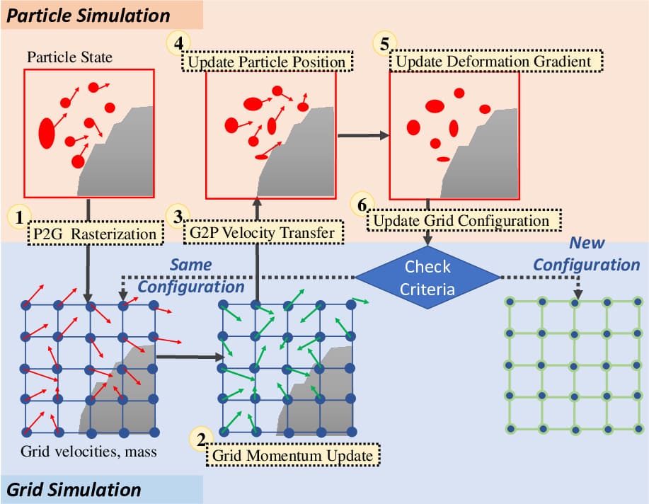
Our method introduces a nodal discretized Lagrangian into hybrid grid-to-particle discretization for MPM and takes advantage of the zero cell-crossing error and zero numerical fracture properties of TLMPM. It also allows for updating the reference configuration in an adaptive manner to ensure robustness during extreme material deformations, such as those arising in fluid simulations. In contrast to prior MPM formulations (see equations (6) and (7)), our method adopts adaptive reference configurations (see grids at time in Figure 5) to measure stress, strain, interpolation kernels and their derivatives. Data from particles is first transferred to grids (P2G) in their latest configuration. Next, the forces are evaluated and the velocities are updated on these grids. Subsequently, the updated grid velocities are interpolated back to the particles (G2P) and used to update the particle positions following the APIC method (Jiang et al., 2015). The velocity gradients and deformation gradients are then updated on the particles leveraging information on the grids. Our method uses a novel criterion (see equation (33)) for automatically determining when to update the grid configuration. This prevents data transfers between the particles and grids from accumulating errors as the interpolation functions are only updated when necessary. Figure 6 provides a high-level overview of our method and the essential algorithmic steps are summarized below:
-
(1)
P2G Rasterization: Velocities on particles are reconstructed by first-order Taylor expansion, and mass and momentum from particles at time are transferred to grids at time .
-
(2)
Grid Momentum Update: Grid momentum is updated using explicit or implicit schemes. Note that forces are evaluated with respect to the latest configuration at time .
-
(3)
G2P Velocity Transfer: Use APIC (Jiang et al., 2015) to transfer velocities from the grid to particles.
-
(4)
Update Particle Positions: Particle positions are updated with their new velocities.
-
(5)
Update Particle Deformation Gradients: Use the MLS gradient operator to update the particle deformation gradient and account for plasticity, if it occurs.
-
(6)
Update Grid Configuration: Check if the deformation is extreme according to the update criterion in equation (33). In case of a large deformation, update weights between particles and the grid and the matrices on particles.
4.1. Terminology
We show integration of our arbitrary updated Lagrangian formulation with Kernel-MPM (Stomakhin et al., 2013) in Appendix B and MLS-MPM (Hu et al., 2018) in Section 5. In Kernel-MPM, the interpolation is performed using shape functions and stress divergence is evaluated by derivatives of the shape function, while MLS-MPM utilizes APIC particle-to-grid velocity rasterization and uses MLS shape functions to derive the internal force term. Using these definitions, our terminology for different methods is provided as follows:
-
(1)
Kernel-MPM: In kernel-MPM, we have kernel-EMPM and kernel-TLMPM represent the kernel-MPM in Eulerian and total Lagrangian frameworks, respectively. Kernel-EMPM was presented in (Stomakhin et al., 2013) and kernel-TLMPM was present in (de Vaucorbeil et al., 2020). These two methods can be recovered in our kernel--ULMPM framework by setting for EMPM and for TLMPM.
-
(2)
MLS-MPM: In MLS-MPM, we have MLS-EMPM and MLS-TLMPM represent MLS-MPM in Eulerian and total Lagrangian frameworks, respectively. MLS-EMPM was presented in MLS-MPM (Hu et al., 2018). Besides, MLS-EMPM and MLS-TLMPM can be recovered in MLS--ULMPM by setting for MLS-EMPM and for MLS-TLMPM.
| Particle | Description | Grid |
|---|---|---|
| position | ||
| velocity | ||
| deformation gradient at | ||
| with respect to configuration at | ||
| deformation gradient at | ||
| with respect to configuration at | ||
| deformation gradient at | ||
| with respect to configuration at | ||
| Stress tensor | ||
| volume change at | ||
| with respect to configuration at | ||
| force | ||
| volume | ||
| mass |
5. -ULMPM Formulation
Starting from a nodal Lagrangian formulation, we derive an alternate expression for equation (6) in the hybrid particle-grid framework of MPM. Interestingly, our formulation leads to a new MLS-MPM method (MLS--ULMPM) whose variant recovers MLS-MPM (Hu et al., 2018) in the Eulerian setting. We use subscript to denote quantities on grid nodes, subscript to denote quantities on particles, and subscript to denote the intermediate configuration map. Table 1 summarizes the notation used in this section.
5.1. Grid Setting
We use a global grid that covers the entire computational domain. Each object has its own configuration map that maps points within the object to specific locations in the global grid. To reduce the associated memory overhead, we implement the global grid using sparsity aware data structures (Setaluri et al., 2014).
5.2. P2G Rasterization
In contrast to EMPM, the velocity gradients and weights are all evaluated with respect to the configuration map at time . We use a first order Taylor expansion to reconstruct particle velocities and rasterize particle momentum to the grid as follows:
| (10) |
where and , which is further expanded out in equation (31). The mass/velocity at grid nodes are given by:
| (11) |
We also rasterize particle positions to the grid to simplify the theoretical derivations for the deformation gradient in equation (29) and internal forces in equation (19) as shown below:
| (12) |
The idea of introducing a first-order Taylor expansion to enhance velocity rasterization is not new and can also be found in APIC (Jiang et al., 2015) and MLS-MPM (Hu et al., 2018).
5.3. Grid Momentum Update
5.3.1. Nodal Lagrangian
We interpolate the Lagrangian at grid node using values associated with its nearby particles as follows:
| (13) |
Substituting the expression for to equations (4) and (8) gives:
-
(1)
Kinetic term:
(14) -
(2)
Deformation term:
(15) where .
Thus, the equation of motion for grid node at time is given by:
| (16) |
The reader may have noticed that an explicit expression of equation (16) relies on a concrete formulation of and its derivative . For example, in kernel-MPM (Stomakhin et al., 2013), the shape function is unitized to simplify the internal force evaluation in equation (16) (see Appendix B).
5.3.2. MLS-based gradient operator
We use the gradient operator based on moving least squares (MLS) that was proposed in (Xue et al., 2019) (see Appendix A) that locally minimizes the error of a certain position over its neighborhood. Following the same notation in equation (16), the deformation gradient of particle at time relative to an arbitrary configuration map at time is given as:
| (17) |
where .
5.3.3. Evaluation of
5.3.4. MPM Equation of Motion with Arbitrary Updated Lagrangian
Substituting equation (18) to equation (16) yields the following equation of motion for grid node at time :
| (19) |
where and . and are given by:
We take advantage of equation (12) to simplify the term in equation (19) as follows:
Setting , equation (19) can be rewritten as follows:
| (20) |
Equation (20) is a general MPM formulation that allows the use of arbitrary intermediate configurations. It spans from total Lagrangian formulations to updated Lagrangian formulations. Specifically:
-
(1)
Setting yields total Lagrangian MPM:
(21) -
(2)
Setting yields Eulerian MPM:
(22)
In the total Lagrangian formulation, there is no need to update , , , and matrices in equation (21), while they require an update at every time step in the Eulerian setting (see equation (22)).


5.4. Grid Velocity and Position Update
With explicit time stepping, the velocity is updated as , where is given by:
| (23) |
For a semi-implicit update, we follow (Stomakhin et al., 2013; Hu et al., 2018) and take an implicit step on the velocity update by utilizing the Hessian of with respective to . The action of this Hessian on an arbitrary increment is given as follows:
| (24) |
where is given by:
| (25) |
We linearize the implicit system with one step of Newton’s method, which provides the following symmetric system for :
| (26) |
where is the identity matrix and is given in equation (23). We update rasterized positions at grid nodes as shown below:
| (27) |
5.5. G2P Velocity and Position Transfer
5.6. Update Particle Deformation Gradients
We first update particle deformation gradients with respect to the latest configuration at time and use the following MLS-based gradient operator (see equation (17)):
| (29) |
Substituting and to equation (29) gives:
| (30) |
where is given by:
| (31) |
Using the chain rule, the update for is given by:
| (32) |
.
5.7. Update Grid Configuration Map
We designed the configuration update criterion based on an intuitive assumption that more severe deformation is accompanied with large change of in the next time step with respect to the latest configuration . Using this observation, our criterion is defined as a measure for the amount of particle deformation as follows:
| (33) |
where and . We mark particles with as indicators where large deformation is taking place and count the total amount of marked particles (). If , where is the total number of particles, we update , , and . Otherwise, these variables remain the same until a new update occurs. and are user-defined parameters to adjust the update frequency.
5.8. Similarities with MLS-EMPM and APIC
While our -ULMPM framework is new to computer graphics, setting for the configuration map shares some similarities with MLS-EMPM (Hu et al., 2018) and APIC (Jiang et al., 2015). We prove that the MLS-gradient of velocity is equivalent to the APIC-gradient of velocity by leveraging the properties of interpolation weights (Jiang et al., 2017b) as follows:
| (34) |
Our internal force in equation (23) has the same pattern as that in original MLS-EMPM (Hu et al., 2018), which is derived from the weak-form element-free Galerkin (EFG) framework. The matrices are simplified by for quadratic and for cubic . This simplification comes from the properties of splines, and is not generally true for other interpolation functions.
6. Results
Accompanying this article, we open-source our code for running 3D examples with our proposed -ULMPM framework (see Section 5). MLS-based MPM, including MLS-EMPM, MLS-TLMPM, and MLS--ULMPM, was applied to simulate all our 3D simulations. Besides the advantage of removing numerical fracture and the cell-crossing instability in solid and fluid simulations, -ULMPM has the practical convenience of using the same numerical implementation to adaptively update the configuration map, without having to switch between TLMPM and EMPM. We use the example of a falling elastic ball (see Figure 5) to evaluate the computational cost of explicit (see equation (23)) and implicit (see equation (26)) Euler schemes. As shown in the first two rows of Table 2, the computational cost of these two schemes are comparable. Given the low stiffness in the materials, we utilize the explicit Euler scheme in all our 3D examples and did not experience any need for excessively small time steps. For our 3D solid simulations, we set and , and observed that no configuration update was required, showing that -ULMPM inherits the advantage of TLMPM for solid simulation. Due to foreseeable large deformations that arise when simulating fluid-like materials, such as water splashes and snow scattering, we set and to update the configuration maps more frequently. Even so, our -ULMPM scheme reduces the configuration update overhead by – in fluid-like simulations (see Table 3), compared to standard EMPM. Table 2 summarizes the specific timings for all our examples.
| Simulation | Time | Machine | Grid | Particle |
|---|---|---|---|---|
| 2D Elastic ball (Fig.5) | 0.0148 | 1 | 16.4K | 20K |
| 2D Elastic ball (implicit) | 0.0165 | 1 | 16.4K | 20K |
| 2D Rotation (Fig.2(1st row)) | 0.0571 | 1 | 16.4K | 42K |
| 2D Rotation (Fig. 2(2nd row)) | 0.0571 | 1 | 16.4K | 42K |
| 2D Rotation (Fig. 2(3rd row)) | 0.0571 | 1 | 16.4K | 42K |
| 2D Droplet (Fig. 3(1st row)) | 0.0154 | 1 | 16.4K | 5K |
| 2D Droplet (Fig. 3(2nd row)) | 0.0108 | 1 | 16.4K | 5K |
| 2D Droplet (Fig. 3(3rd row)) | 0.0194 | 1 | 16.4K | 5K |
| 2D Droplet (Fig. 3(4th row)) | 0.0146 | 1 | 16.4K | 5K |
| 2D Droplet (Fig. 3(5th row)) | 0.0199 | 1 | 16.4K | 5K |
| Twisting bar (Fig.4(1st row)) | 0.627 | 1 | 1.0M | 193.3K |
| Twisting bar (Fig.4(2nd row)) | 0.624 | 1 | 1.0M | 193.3K |
| Twisting bar (Fig.7(1st row)) | 0.125 | 2 | 131.1K | 48.3K |
| Twisting bar (Fig.7(2nd row)) | 0.124 | 2 | 131.1K | 48.3K |
| Stretchy yo-yo (Fig.10(1st row)) | 1.314 | 2 | 4.2M | 179.3K |
| Stretchy yo-yo (Fig.10(2nd row)) | 1.310 | 2 | 4.2M | 179.3K |
| Snow bunny (Fig.8) | 0.965 | 2 | 524.3K | 116.3K |
| Snow bunny (EMPM in video) | 0.971 | 2 | 523.4K | 116.3K |
| Water bunny (Fig.9) | 0.341 | 2 | 2.1M | 96.3K |
| Water bunny (EMPM in video) | 0.381 | 2 | 2.1M | 96.3K |
| FSI (Fig.11(1st row)) | 0.934 | 1 | 4.2M | 169.1K |
| FSI (Fig.11(2nd row)) | 0.939 | 1 | 4.2M | 169.1K |
| Simulation | Cost | |||
|---|---|---|---|---|
| Snow bunny (-ULMPM in Fig.8) | 0.01 | 0.01 | 24.33 | 0.112 |
| Snow bunny (EMPM in video) | N/A | N/A | 104 | 0.479 |
| Water bunny (-ULMPM in Fig.9) | 0.01 | 0.01 | 3.31 | 0.021 |
| Water bunny (EMPM in video) | N/A | N/A | 104 | 0.662 |
6.1. 2D Simulations for Solids and Fluids
6.1.1. Numerical fracture and cell-crossing instability
We simulated a 2D rotating hyperelastic plate to demonstrate that EMPM suffers from the cell-crossing instability, which leads to severe numerical fractures, while TLMPM can completely eliminate these artifacts. Figure 2 shows that our -ULMPM framework and TLMPM integrated with MLS-MPM captures the appealing hyperelastic rotation, preserving the angular momentum for long simulation periods while completely eliminating numerical fractures. However, traditional MLS-MPM (Hu et al., 2018) that uses an Eulerian approach suffers from severe numerical fractures when large deformations occur.
We quantitatively evaluate the spatial accuracy of our method on the rotating hyperelastic plate example by varying the grid resolution . We utilized numerical results with resolution as the benchmark solution (see Figure 2) and discretize sampling examples with spatial resolution for the grid. We fixed the particle number for each case and ran simulations up to a total simulation time of with a time step size of . The error for numerical simulations is defined as:
| (35) |
where is the variable evaluated by lower grid resolutions, while is the value at resolution (benchmark). Figure 12 shows the convergence plots for the average particle displacement and velocity for -ULMPM integrated with MLS-MPM , -ULMPM integrated with MLS-MPM , -ULMPM integrated with MLS-MPM (black) , and -ULMPM integrated with kernel-MPM , where -ULMPM () recovers TLMPM and -ULMPM () recovers EMPM, as described in Section 5. In general, TLMPM can produce more accurate simulations since the cell-crossing error is completely eliminated, while EMPM fails to converge when the cell-crossing error is significant. -ULMPM with exhibits second-order accuracy while its integration with MLS-MPM has higher solution accuracy than that with kernel-MPM.
6.1.2. 2D droplet
We ran several simulations of falling droplets to compare our implementations in the -ULMPM framework. As shown in Figure 3, although TLMPM has benefits over EMPM for solid simulations (see Figure 2), it fails to achieve detailed free surfaces in fluid simulations, as shown in Figure 3, since the topology changes significantly in fluid-like simulations. -ULMPM automatically updates configuration maps to produce similar fluid dynamics as EMPM and captures rich interactions. Moreover, our integration with MLS-MPM (see Section 5) yields more energetic behavior compared to an integration with kernel-MPM (see Appendix B).
6.2. Bar Twisting
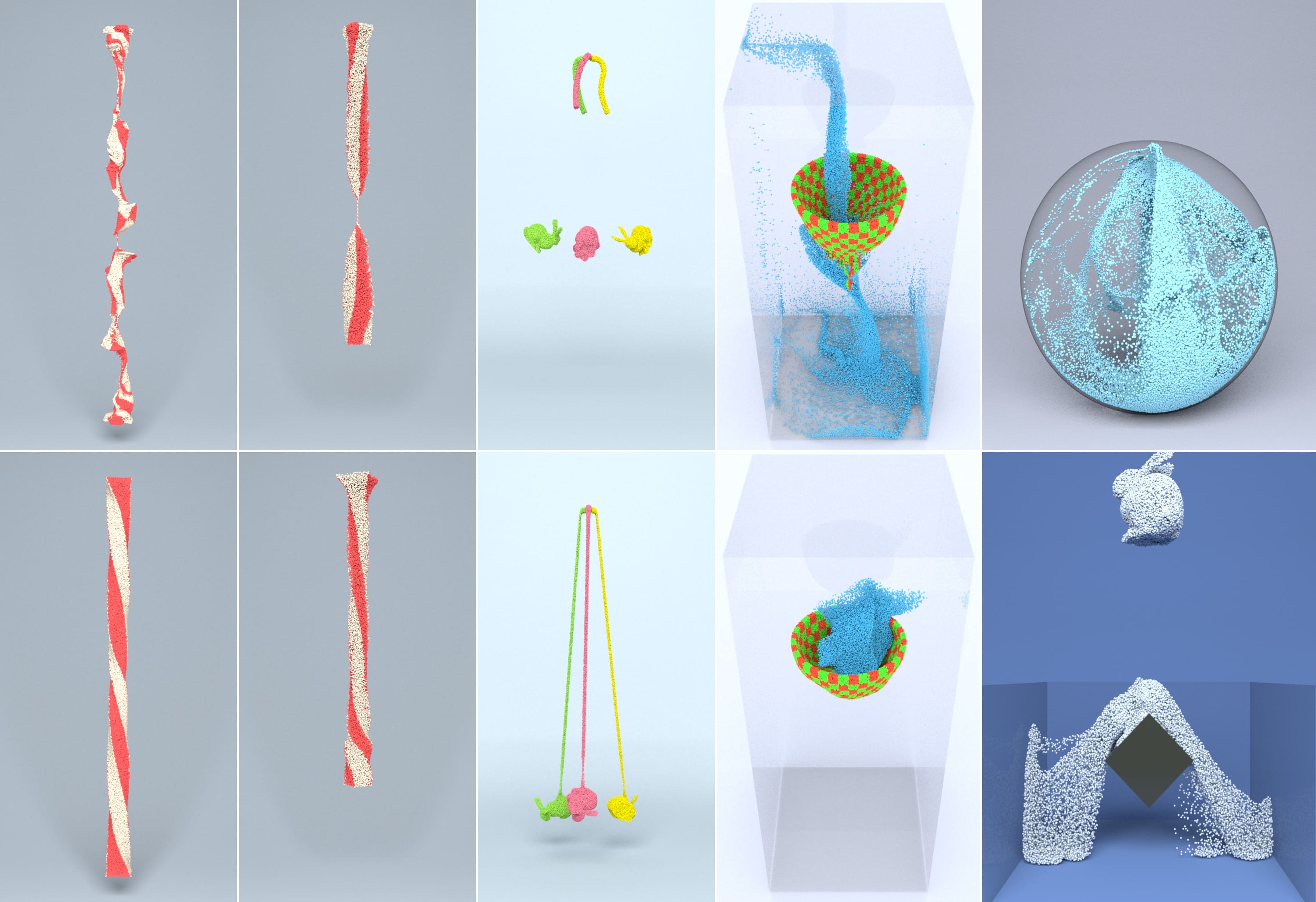
We imposed torsion and stretch boundary conditions at the two ends of a hyperelastic beam to showcase that -ULMPM allows large deformations in solids without non-physical fractures. As shown in Figure 4, traditional EMPM fails to preserve the shape of the beam during the twisting and pulling, while -ULMPM can readily handle the challenging invertible elasticity when one end of the beam is released after twisting. Figure 7 shows that -ULMPM is capable of robustly recovering the beam shape after extreme elastic deformations, while particles in EMPM cluster into one irreversible (or plastic) thin string blocking the “recovery” of elasticity.
6.3. Stretchy Yo-Yo
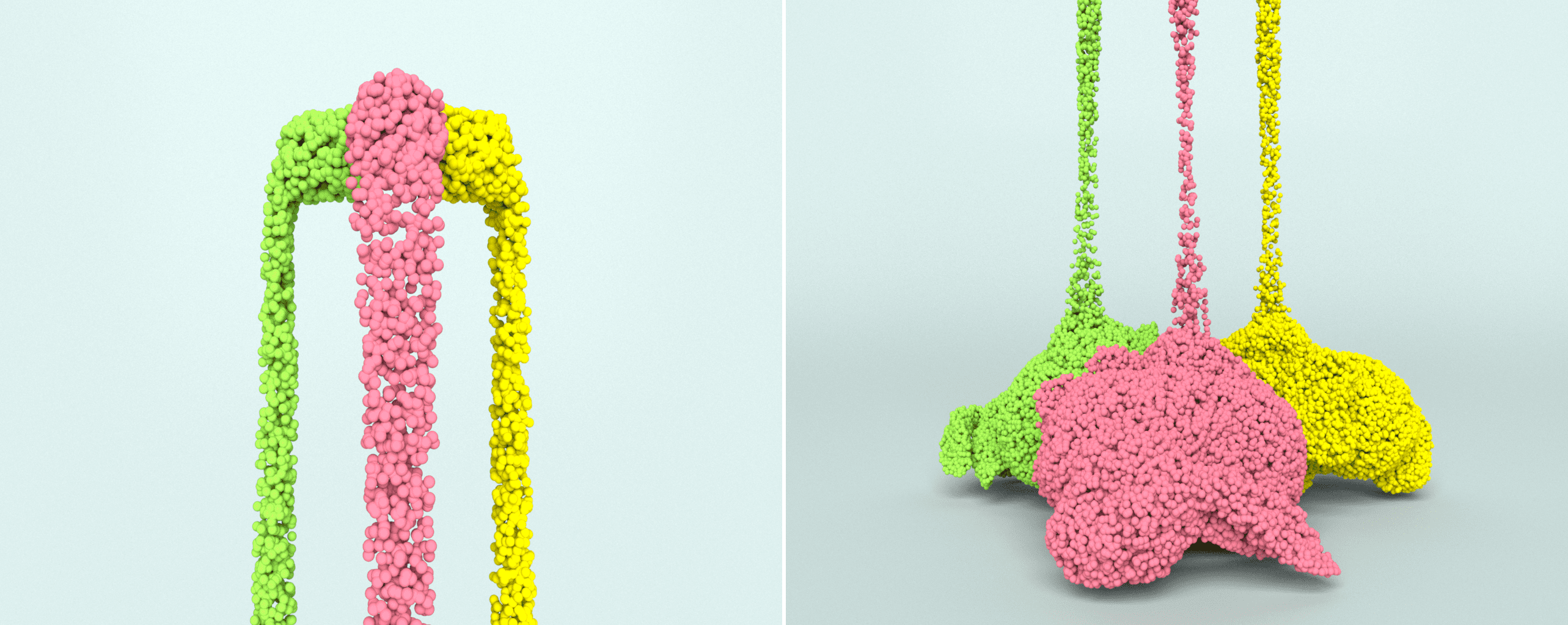
Next, we tossed a stretchy Stanford bunny yo-yo with gravity forces. Our -ULMPM hyperelastic bunny demonstrates rich elastic responses and realistic bouncing dynamics, while EMPM breaks due to severe numerical fracture (see Figure 10). Our -ULMPM framework can perfectly handle hyperelastic deformation under severe bending (see Figure 13 (left)) and stretching (see Figure 13 (right)).
6.4. Fluid-like Bunny Simulation
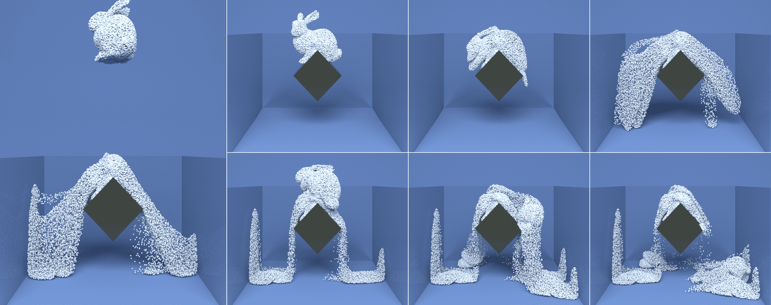
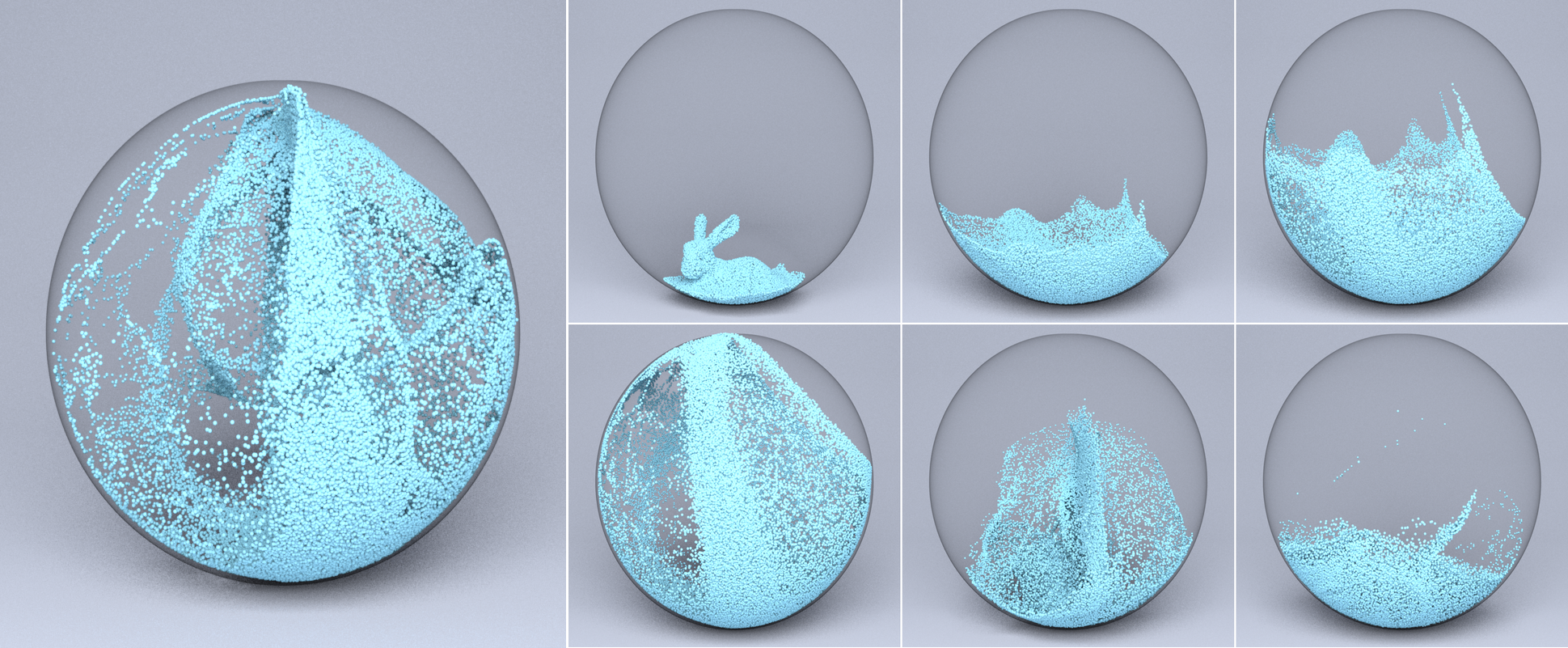
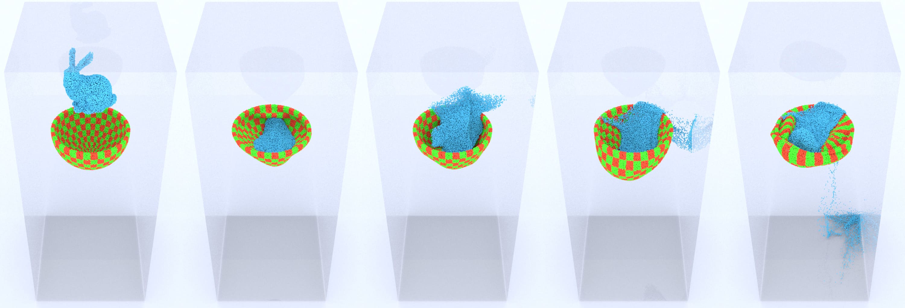
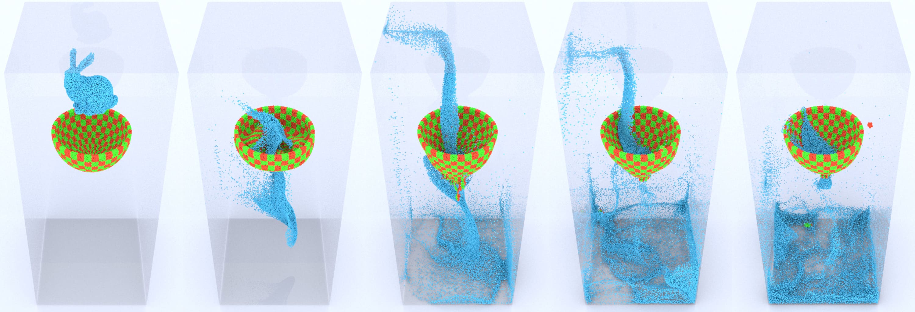
We simulated the fluid-like behavior of different materials using our -ULMPM framework, as described in Section 5, such as elastoplastic snow (Stomakhin et al., 2013) and weakly compressible water. We dropped two copies of the snow Stanford bunny with different orientations to a solid wedge, as shown in Figure 8. -ULMPM captures the vivid snow smashing and scattering after the bunnies fall on the wedge, similar to its Eulerian counterparts proposed in prior works (Stomakhin et al., 2013) (see side-by-side comparisons in our video). We simulated a water Stanford bunny falling inside a spherical container (see Figure 9), showing the extreme large deformations and energetic splashes. -ULMPM does not update the configuration maps at each time step, in contrast to EMPM, so it is naturally more efficient in fluid-like simulations (see Table 3).
6.5. Fluid-Structure Interaction
Our -ULMPM framework can also simulate realistic fluid-structure interaction problems, as shown in Figure 11.
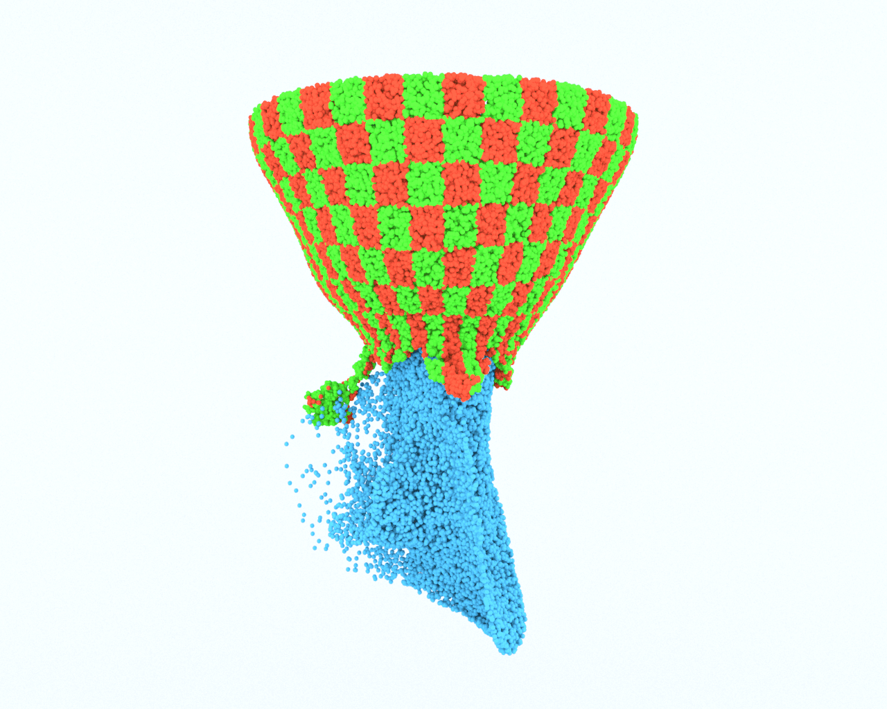
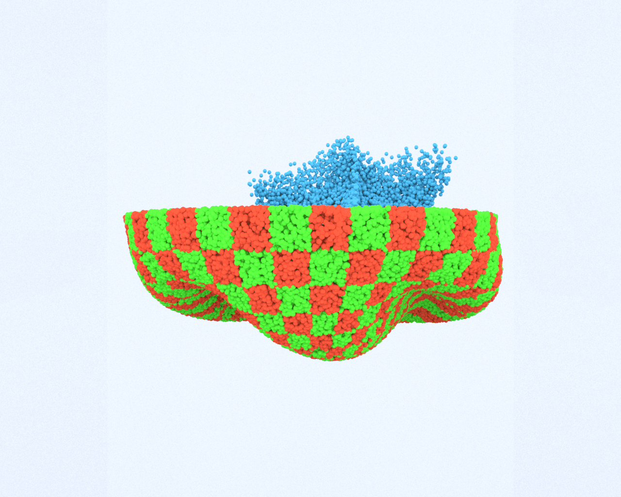
We dropped a water Stanford bunny to a hyperelastic bowl. -ULMPM captures rich fluid-structure interactions, displaying advantages of both TLMPM and EMPM (see Figure 14 (right)), and highlighting that -ULMPM can adaptively handle both fluid and solid simulations without having to switch between TLMPM and EMPM. In contrast, EMPM suffers from numerical fractures. As shown in Figure 11, the hyperelastic bowl fractures, causing the water to spill below.
7. Discussion and Conclusion
7.1. Limitations and Future Work
Our model has generated a large number of compelling examples, but there remains much work to be done. Parameters to adjust the configuration update frequency were tuned by hand, and it would be interesting to calibrate them to measured models. Since each object has it own configuration map, we only briefly investigated contact by projecting particle positions to a global grid and processing grid-based collisions (Stomakhin et al., 2013). By doing this, we observed slight self-penetration in the 3D twisting beam example (see Figure 4). This could be addressed by further introducing contact algorithms, such as (Jiang et al., 2017a; Han et al., 2019). While we did not experience a need for excessively small time steps given the low stiffness of the materials we considered, deforming materials with high wave speed, such as steel, could benefit from a fully implicit discretization. Though side-to-side comparisons with Eulerian MLS-MPM shows that our -ULMPM framework produces similar fluid-like dynamics as EMPM and captures rich interactions, a slight energy loss in -ULMPM framework was observed. This could be addressed by introducing more accurate configuration update criteria. Finally, while our focus was on the material responses of water, snow, and hyperelastic solids, it would be interesting to investigate other materials and multi-physics coupling problems with -ULMPM.
7.2. Conclusion
We proposed an arbitrary updated Lagrangian Material Point Method (-ULMPM), which combines advantages of Total Lagrangian frameworks (de Vaucorbeil and Nguyen, 2021; de Vaucorbeil et al., 2020) and Eulerian frameworks (Stomakhin et al., 2013; Hu et al., 2018) in an adaptive fashion. -ULMPM avoids the cell-crossing instability and numerical fracture in solid simulations, while still allowing for large deformations that arise in fluid-like simulations. It can be easily integrated with any existing MPM framework and builds a foundation for devising various MPM schemes, such as PolyPIC (Fu et al., 2017), for enhanced accuracy and visual vividness.
References
- (1)
- Bardenhagen (2002) SG Bardenhagen. 2002. Energy conservation error in the material point method for solid mechanics. J. Comput. Phys. 180, 1 (2002), 383–403.
- Bardenhagen and Kober (2004) Scott G Bardenhagen and Edward M Kober. 2004. The generalized interpolation material point method. Computer Modeling in Engineering and Sciences 5, 6 (2004), 477–496.
- Brackbill et al. (1988) Jeremiah U Brackbill, Douglas B Kothe, and Hans M Ruppel. 1988. FLIP: a low-dissipation, particle-in-cell method for fluid flow. Computer Physics Communications 48, 1 (1988), 25–38.
- d. Goes et al. (2015) F. d. Goes, C. Wallez, J. Huang, D. Pavlov, and M. Desbrun. 2015. Power Particles: An Incompressible Fluid Solver Based on Power Diagrams. ACM Trans Graph 34, 4, Article 50 (2015).
- Daviet and Bertails-Descoubes (2016) Gilles Daviet and Florence Bertails-Descoubes. 2016. A semi-implicit material point method for the continuum simulation of granular materials. ACM Transactions on Graphics (TOG) 35, 4 (2016), 1–13.
- de Vaucorbeil and Nguyen (2021) Alban de Vaucorbeil and Vinh Phu Nguyen. 2021. Modelling contacts with a total Lagrangian material point method. Computer Methods in Applied Mechanics and Engineering 373 (2021), 113503.
- de Vaucorbeil et al. (2020) Alban de Vaucorbeil, Vinh Phu Nguyen, and Christopher R Hutchinson. 2020. A Total-Lagrangian Material Point Method for solid mechanics problems involving large deformations. Computer Methods in Applied Mechanics and Engineering 360 (2020), 112783.
- Desbrun and Gascuel (1996) Mathieu Desbrun and Marie-Paule Gascuel. 1996. Smoothed Particles: A new paradigm for animating highly deformable bodies. In Computer Animation and Simulation ’96. 61–76.
- Ding et al. (2019) Mengyuan Ding, Xuchen Han, Stephanie Wang, Theodore F Gast, and Joseph M Teran. 2019. A thermomechanical material point method for baking and cooking. ACM Transactions on Graphics (TOG) 38, 6 (2019), 1–14.
- Erleben (2013) Kenny Erleben. 2013. Numerical Methods for Linear Complementarity Problems in Physics-Based Animation. In ACM SIGGRAPH 2013 Courses (SIGGRAPH ’13). Article 8, 42 pages.
- Fang et al. (2019) Yu Fang, Minchen Li, Ming Gao, and Chenfanfu Jiang. 2019. Silly rubber: an implicit material point method for simulating non-equilibrated viscoelastic and elastoplastic solids. ACM Transactions on Graphics (TOG) 38, 4 (2019), 1–13.
- Fang et al. (2020) Yu Fang, Ziyin Qu, Minchen Li, Xinxin Zhang, Yixin Zhu, Mridul Aanjaneya, and Chenfanfu Jiang. 2020. IQ-MPM: an interface quadrature material point method for non-sticky strongly two-way coupled nonlinear solids and fluids. ACM Transactions on Graphics (TOG) 39, 4 (2020), 51–1.
- Fei et al. (2018) Y. Fei, C. Batty, E. Grinspun, and C. Zheng. 2018. A Multi-scale Model for Simulating Liquid-fabric Interactions. ACM Trans Graph 37, 4 (2018), 51:1–51:16.
- Fei et al. (2017) Y. Fei, H. T. Maia, C. Batty, C. Zheng, and E. Grinspun. 2017. A Multi-Scale Model for Simulating Liquid-Hair Interactions. ACM Trans Graph 36, 4, Article 56 (2017).
- Fu et al. (2017) Chuyuan Fu, Qi Guo, Theodore Gast, Chenfanfu Jiang, and Joseph Teran. 2017. A polynomial particle-in-cell method. ACM Transactions on Graphics (TOG) 36, 6 (2017), 1–12.
- Gao et al. (2018a) M. Gao, A. Pradhana, X. Han, Q. Guo, G. Kot, E. Sifakis, and C. Jiang. 2018a. Animating fluid sediment mixture in particle-laden flows. ACM Trans Graph 37, 4 (2018), 149.
- Gao et al. (2017) Ming Gao, Andre Pradhana Tampubolon, Chenfanfu Jiang, and Eftychios Sifakis. 2017. An adaptive generalized interpolation material point method for simulating elastoplastic materials. ACM Transactions on Graphics (TOG) 36, 6 (2017), 1–12.
- Gao et al. (2018b) M. Gao, X. Wang, K. Wu, A. Pradhana, E. Sifakis, C. Yuksel, and C. Jiang. 2018b. GPU Optimization of Material Point Methods. ACM Trans Graph 37, 6, Article 254 (2018), 12 pages.
- Gaume et al. (2018) J. Gaume, T. Gast, J. Teran, A. v. Herwijnen, and C. Jiang. 2018. Dynamic anticrack propagation in snow. Nature Comm 9, 1 (2018), 3047.
- Han et al. (2019) Xuchen Han, Theodore F Gast, Qi Guo, Stephanie Wang, Chenfanfu Jiang, and Joseph Teran. 2019. A hybrid material point method for frictional contact with diverse materials. Proceedings of the ACM on Computer Graphics and Interactive Techniques 2, 2 (2019), 1–24.
- Hegemann et al. (2013) J. Hegemann, C. Jiang, C. Schroeder, and J. Teran. 2013. A level set method for ductile fracture. In Proc ACM SIGGRAPH/Eurograp Symp Comp Anim. 193–201.
- Hu et al. (2018) Yuanming Hu, Yu Fang, Ziheng Ge, Ziyin Qu, Yixin Zhu, Andre Pradhana, and Chenfanfu Jiang. 2018. A moving least squares material point method with displacement discontinuity and two-way rigid body coupling. ACM Transactions on Graphics (TOG) 37, 4 (2018), 1–14.
- Hu et al. (2019) Y. Hu, J. Liu, A. Spielberg, J. B. Tenenbaum, W. T. Freeman, J. Wu, D. Rus, and W. Matusik. 2019. ChainQueen: A Real-Time Differentiable Physical Simulator for Soft Robotics. Proc of the Int Conf on Robotics and Automation (ICRA) (2019), 6265–6271.
- Jiang et al. (2017a) Chenfanfu Jiang, Theodore Gast, and Joseph Teran. 2017a. Anisotropic elastoplasticity for cloth, knit and hair frictional contact. ACM Transactions on Graphics (TOG) 36, 4 (2017), 1–14.
- Jiang et al. (2015) C. Jiang, C. Schroeder, A. Selle, J. Teran, and A. Stomakhin. 2015. The affine particle-in-cell method. ACM Trans Graph 34, 4 (2015), 51:1–51:10.
- Jiang et al. (2017b) Chenfanfu Jiang, Craig Schroeder, and Joseph Teran. 2017b. An angular momentum conserving affine-particle-in-cell method. J. Comput. Phys. 338 (2017), 137–164.
- Jiang et al. (2016) Chenfanfu Jiang, Craig Schroeder, Joseph Teran, Alexey Stomakhin, and Andrew Selle. 2016. The material point method for simulating continuum materials. In ACM SIGGRAPH 2016 Courses. 1–52.
- Klár et al. (2016) Gergely Klár, Theodore Gast, Andre Pradhana, Chuyuan Fu, Craig Schroeder, Chenfanfu Jiang, and Joseph Teran. 2016. Drucker-prager elastoplasticity for sand animation. ACM Transactions on Graphics (TOG) 35, 4 (2016), 1–12.
- Liu et al. (2008) MB Liu, GR Liu, and Z Zong. 2008. An overview on smoothed particle hydrodynamics. International Journal of Computational Methods 5, 01 (2008), 135–188.
- Macklin et al. (2014) M. Macklin, M. Muller, N. Chentanez, and T. Kim. 2014. Unified particle physics for real-time applications. ACM Trans Graph 33, 4 (2014), 153:1–153:12.
- McAdams et al. (2009) A. McAdams, A. Selle, K. Ward, E. Sifakis, and J. Teran. 2009. Detail Preserving Continuum Simulation of Straight Hair. ACM Trans Graph 28, 3 (2009), 62:1–62:6.
- Müller et al. (2007) M. Müller, B. Heidelberger, M. Hennix, and J. Ratcliff. 2007. Position Based Dynamics. J Vis Comm Imag Repre 18, 2 (2007), 109–118.
- Müller et al. (2004) Matthias Müller, Richard Keiser, Andrew Nealen, Mark Pauly, Markus Gross, and Marc Alexa. 2004. Point based animation of elastic, plastic and melting objects. In Proceedings of the 2004 ACM SIGGRAPH/Eurographics symposium on Computer animation. 141–151.
- Narain et al. (2010) R. Narain, A. Golas, and M. Lin. 2010. Free-flowing granular materials with two-way solid coupling. ACM Trans Graph 29, 6 (2010), 173:1–173:10.
- Patkar et al. (2013) S. Patkar, M. Aanjaneya, D. Karpman, and R. Fedkiw. 2013. A hybrid Lagrangian-Eulerian formulation for bubble generation and dynamics. In Proc ACM SIGGRAPH/Eurograp Symp Comp Anim. 105–114.
- Ram et al. (2015) Daniel Ram, Theodore Gast, Chenfanfu Jiang, Craig Schroeder, Alexey Stomakhin, Joseph Teran, and Pirouz Kavehpour. 2015. A material point method for viscoelastic fluids, foams and sponges. In Proceedings of the 14th ACM SIGGRAPH/Eurographics Symposium on Computer Animation. 157–163.
- Sadeghirad et al. (2011) Alireza Sadeghirad, Rebecca M Brannon, and Jeff Burghardt. 2011. A convected particle domain interpolation technique to extend applicability of the material point method for problems involving massive deformations. International Journal for numerical methods in Engineering 86, 12 (2011), 1435–1456.
- Setaluri et al. (2014) Rajsekhar Setaluri, Mridul Aanjaneya, Sean Bauer, and Eftychios Sifakis. 2014. SPGrid: A Sparse Paged Grid Structure Applied to Adaptive Smoke Simulation. ACM Trans. Graph. 33, 6, Article 205 (2014), 12 pages.
- Shabana (2018) Ahmed A Shabana. 2018. Computational continuum mechanics. John Wiley & Sons.
- Sifakis and Barbic (2012) E. Sifakis and J. Barbic. 2012. FEM Simulation of 3D Deformable Solids: A Practitioner’s Guide to Theory, Discretization and Model Reduction. In ACM SIGGRAPH 2012 Courses. Article 20.
- Sifakis et al. (2008) E. Sifakis, S. Marino, and J. Teran. 2008. Globally Coupled Collision Handling Using Volume Preserving Impulses. In Symp. Comp. Anim. 147–153.
- Sin et al. (2009) Funshing Sin, Adam W. Bargteil, and Jessica K. Hodgins. 2009. A Point-Based Method for Animating Incompressible Flow. In Proceedings of the 2009 ACM SIGGRAPH/Eurographics Symposium on Computer Animation (SCA ’09). 247–255.
- Steffen et al. (2008) Michael Steffen, Robert M Kirby, and Martin Berzins. 2008. Analysis and reduction of quadrature errors in the material point method (MPM). International journal for numerical methods in engineering 76, 6 (2008), 922–948.
- Stomakhin et al. (2013) Alexey Stomakhin, Craig Schroeder, Lawrence Chai, Joseph Teran, and Andrew Selle. 2013. A material point method for snow simulation. ACM Transactions on Graphics (TOG) 32, 4 (2013), 1–10.
- Stomakhin et al. (2014) Alexey Stomakhin, Craig Schroeder, Chenfanfu Jiang, Lawrence Chai, Joseph Teran, and Andrew Selle. 2014. Augmented MPM for phase-change and varied materials. ACM Transactions on Graphics (TOG) 33, 4 (2014), 1–11.
- Su et al. (2021) Tao Su, Haozhe Xue, , Chengguizi Han, Chenfanfu Jiang, and Mridul Aanjaneya. 2021. A Unified Second-Order Accurate in Time MPM Formulation for Simulating Viscoelastic Liquids with Phase Change. ACM Trans. Graph. 40, 4, Article 119 (Aug. 2021), 18 pages.
- Sulsky et al. (1994) Deborah Sulsky, Zhen Chen, and Howard L Schreyer. 1994. A particle method for history-dependent materials. Computer methods in applied mechanics and engineering 118, 1-2 (1994), 179–196.
- Sulsky et al. (1995) Deborah Sulsky, Shi-Jian Zhou, and Howard L Schreyer. 1995. Application of a particle-in-cell method to solid mechanics. Computer physics communications 87, 1-2 (1995), 236–252.
- Tampubolon et al. (2017) Andre Pradhana Tampubolon, Theodore Gast, Gergely Klár, Chuyuan Fu, Joseph Teran, Chenfanfu Jiang, and Ken Museth. 2017. Multi-species simulation of porous sand and water mixtures. ACM Transactions on Graphics (TOG) 36, 4 (2017), 1–11.
- Wallstedt and Guilkey (2007) PC Wallstedt and JE Guilkey. 2007. Improved velocity projection for the material point method. Computer Modeling in Engineering and Sciences 19, 3 (2007), 223.
- Wolper et al. (2020) Joshuah Wolper, Yunuo Chen, Minchen Li, Yu Fang, Ziyin Qu, Jiecong Lu, Meggie Cheng, and Chenfanfu Jiang. 2020. AnisoMPM: Animating Anisotropic Damage Mechanics. ACM Trans. Graph. 39, 4, Article 37 (2020), 16 pages.
- Wolper et al. (2019) Joshuah Wolper, Yu Fang, Minchen Li, Jiecong Lu, Ming Gao, and Chenfanfu Jiang. 2019. CD-MPM: continuum damage material point methods for dynamic fracture animation. ACM Transactions on Graphics (TOG) 38, 4 (2019), 1–15.
- Xue et al. (2020) Tao Xue, Haozhe Su, Chengguizi Han, Chenfanfu Jiang, and Mridul Aanjaneya. 2020. A novel discretization and numerical solver for non-fourier diffusion. ACM Transactions on Graphics (TOG) 39, 6 (2020), 1–14.
- Xue et al. (2019) Tao Xue, Xiaobing Zhang, and Kumar K Tamma. 2019. A non-local dissipative Lagrangian modelling for generalized thermoelasticity in solids. Applied Mathematical Modelling 73 (2019), 247–265.
- Yue et al. (2015) Y. Yue, B. Smith, C. Batty, C. Zheng, and E. Grinspun. 2015. Continuum foam: a material point method for shear-dependent flows. ACM Trans Graph 34, 5 (2015), 160:1–160:20.
- Yue et al. (2018) Yonghao Yue, Breannan Smith, Peter Yichen Chen, Maytee Chantharayukhonthorn, Ken Kamrin, and Eitan Grinspun. 2018. Hybrid Grains: Adaptive Coupling of Discrete and Continuum Simulations of Granular Media. ACM Trans. Graph. 37, 6, Article 283 (2018), 19 pages.
- Zhu and Bridson (2005) Yongning Zhu and Robert Bridson. 2005. Animating sand as a fluid. ACM Transactions on Graphics (TOG) 24, 3 (2005), 965–972.
- Zienkiewicz et al. (1977) Olgierd Cecil Zienkiewicz, Robert Leroy Taylor, Perumal Nithiarasu, and JZ Zhu. 1977. The finite element method. Vol. 3. McGraw-hill London.
Appendix A MLS Gradient
Consider a domain () in Euclidean space . Let denote the geometric position of a certain point in the domain and denote another point which is close to the position . Therefore, any physical quantity at each point in space can be defined as and following a first-order Taylor approximation gives:
| (36) |
where . A weighted error of equation (36) is defined within its associated domain as follows:
| (37) |
where represents the neighboring domain of ; represents the influence from to and is a function of . To minimize the error and get the best approximation, the Least Squares Technique is exploited by introducing :
| (38) |
Therefore, we have a MLS-gradient operator :
| (39) |
where and its discrete form is given by:
| (40) |
where denotes volume distributed at . Moreover, the derivation of with respect to is given as follows:
| (41) |
where is the Kronecker delta function.
Appendix B -ULMPM Integration with kernel-MPM
We briefly describe the integration of our -ULMPM with traditional MPM (Stomakhin et al., 2013) as follows:
-
(1)
Transfer Particle to Grid.
(42) -
(2)
Update Grid Momentum.
(43) - (3)
-
(4)
Update Particle Deformation Gradient.
(44) where is given by:
(46) By differential chain rule, the update of is given by:
(47)