A Volumetric Approach to Monge’s Optimal Transport on Surfaces

Richard Tsai Department of Mathematics, University of Texas at Austin, Austin, TX, 78712 [email protected] and Axel G. R. Turnquist Department of Mathematics, University of Texas at Austin, Austin, TX, 78712 [email protected]

Abstract.

We propose a volumetric formulation for computing the Optimal Transport problem defined on surfaces in $\mathbb{R}^{3}$ , found in disciplines like optics, computer graphics, and computational methodologies. Instead of directly tackling the original problem on the surface, we define a new Optimal Transport problem on a thin tubular region, $T_{\epsilon}$ , adjacent to the surface. This extension offers enhanced flexibility and simplicity for numerical discretization on Cartesian grids. The Optimal Transport mapping and potential function computed on $T_{\epsilon}$ are consistent with the original problem on surfaces. We demonstrate that, with the proposed volumetric approach, it is possible to use simple and straightforward numerical methods to solve Optimal Transport for $\Gamma=\mathbb{S}^{2}$ and the $2$ -torus.

1. Introduction

We consider computational Optimal Transport problems on smooth hypersurfaces in $\mathbb{R}^{3}$ , with the metric induced by the Euclidean distance in $\mathbb{R}^{3}$ . Our objective is to derive an Optimal Transport problem and solve the corresponding Monge-Ampère-like Optimal Transport partial differential equations in a small neighborhood around the hypersurface. This volumetric approach brings more flexibility in dealing with surfaces and covariant derivatives.

In recent years, there has been much interest in finding solving Optimal Transport problems on Riemannian manifolds, mostly motivated from applications. These applications can roughly be divided into two categories, the first where the Optimal Transport problem is derived from first principles, and the second where Optimal Transport is used in an ad hoc way as a powerful tool, usually in geometric and statistical analysis.

In freeform optics, a typical goal is to solve for the shape of reflectors or lenses that take a source light intensity to a desired target intensity pattern. The Optimal Transport partial differential equations arise as a consequence of Snell’s law, the optical setup, and the conservation of light intensity. These formulations are inverse problems in which the potential function of Optimal Transport is directly related to the shapes of lenses or reflectors that redirect source light intensities to required target intensities, see [60, 45, 46], which include examples involving Optimal Transport PDE and other example whose formulations are Generated Jacobian Equations. In Section 4, we will perform one example computation for the cost function arising in the reflector antenna problem, see [56] and [57], which is perhaps the most well-known example of such freeform optics problems with an Optimal Transport formulation.

A completely different application arises due to the fact that the solution to the Optimal Transport PDEs, called the potential function, is the Fréchet gradient of the Wasserstein distance; see [48]. The potential function, therefore, has applications in non-parametric methods in inverse problems, where the Wasserstein distance is used as a “fit” for data, see [3], for example.

In the adaptive mesh community, Optimal Transport has been used as a convenient tool for finding a mapping that redistributes mesh node density to a desired target density. The first such methods in the moving mesh methods community were proposed in [58]. It is also used for the more general problem of diffeomorphic density matching on the sphere, where other approaches such as Optimal Information Transport can be used, see [5].

In the statistics community, Optimal Transport has been extensively employed in computing the distance, or interpolating between, probability distributions on manifolds, and also in sampling, since solving the Optimal Transport problem allows one to compute a pushforward mapping for measures. In these situations, using Optimal Transport is not the only available computational tool, but has shown to be useful in these communities for its regularity and metric properties, even when source and target probability measures are not smooth or bounded away from zero.

Many methods in the last ten or so years have been proposed for computing Optimal Transport related quantities on manifolds, such as the Wasserstein distance. Some of the computations were motivated by applications in computer graphics. In [51], for example, the authors computed the Wasserstein-1 distance on manifolds in order to obtain the geodesic distance on complicated shapes, using a finite-element discretization. In [31], the authors used the Benamou-Brenier formulation of Optimal Transport, a continuous “fluid-mechanics” formulation (as opposed to the static formulation presented here), to compute the Optimal Transport distance, interpolation, mapping, and potential functions on a triangulated approximation of the manifold. However, straightforward implementation using the Brenier-Benamou formulation may suffer from slow convergence. Various authors have successfully employed semi-discrete Optimal Transport methods to Optimal Transport computations on surfaces, where the source measure is a sum of Dirac delta measures and the target measure is continuous. The resulting mapping of such semi-discrete Optimal Transport problems is related to a weighted power diagram of the locations of the source Dirac delta measures. In [11], the authors constructed power diagrams on the sphere to solve the reflector antenna problem, with cost function $c(x,y)=-\log(1-x\cdot y)$ . In [14], the authors utilized a semi-discrete Optimal Transport computation to redistribute the local area of a mesh on the sphere, using the cost function $c(x,y)=\log(x\cdot y)$ . In [38], the authors designed an algorithm to compute the distance between surfaces in $\mathbb{R}^{3}$ and point clouds, using the cost function $c(x,y)=\left\|x-y\right\|^{2}$ , where $\left\|\cdot\right\|$ denotes the Euclidean distance.

We now briefly review methods for solving Optimal Transport problems on surfaces. One common approach to developing numerical methods for surface problems starts with triangularization of the manifold. Recently, in the paper [61], mean-field games were discretized and solved on manifolds using triangularization, of which the Benamou-Brenier formulation of Optimal Transport (using the squared geodesic cost function) is a subcase. One of the great challenges of applying traditional finite element methods to Optimal Transport PDE is the fact that they are not in divergence form. Thus, the analysis becomes very challenging, but, nevertheless, considerable work has been done for this in the Euclidean case with the Monge-Ampère PDE, see, for example, the work done in [7]. It is also not simple to design higher-order schemes, in contrast to simple finite-differences on a Cartesian grid where it is very simple to design high-order discretizations.

There is another general approach to approximating PDE on manifolds, which is done by locally approximating both the manifold and the function to be computed via polynomials using a moving least squares method, originally proposed in [32]. These polynomial approximations are computed in a computational neighborhood. Thus far, these methods have not been applied to solving Optimal Transport PDE on the sphere.

The closest point method was originally proposed in [47] (see also [35]), where the solution of certain PDE are extended to be constant via a closest point map in a small neighborhood of the manifold and all derivatives are then computed using finite differences on a Cartesian grid. However, for our purposes, using the closest point operator for the determinant of a Hessian is rather complicated. Furthermore, simply extending the source and target density functions will not necessarily lead to an Optimal Transport problem on the extended domain and extending the cost function via a closest point extension without introducing a penalty in the normal directions will lead to a degenerate PDE. We have decided instead to extend the source and target density functions and compensating using Jacobian term so they remain density functions and extend the cost function with a penalty term. As we will show in Section 3, these choices will naturally lead to a solution which is constant with respect to the closest point map. Also, we will find in Section 3 that our re-formulation leads to a natural new Optimal Transport problem in a tubular neighborhood with natural zero-Neumann boundary conditions which may be of independent interest for the Optimal Transport community.

In this article, instead of solving directly the Monge problem of Optimal Transport defined on $\Gamma$ , we propose solving the equivalent Optimal Transport problem on a narrowband $T_{\epsilon}$ around $\Gamma$ for a special class of probability measures in $T_{\epsilon}$ that is constructed from probability measures on $\Gamma$ , and with a class of cost functions that is derived from cost functions on $\Gamma$ . Similar to [36], our approach in this paper is to reformulate the variational formulation of the problem on the manifold, which is done in Section 3. It relies on the fact that the extension presented in Section 3 is itself an Optimal Transport problem, and so the usual techniques for the PDE formulation of Optimal Transport are used to formulate the PDE on the tubular neighborhood $T_{\epsilon}$ . We will demonstrate, however, that solving this new Optimal Transport problem in $T_{\epsilon}$ will not require that we take thickness of the narrowband to zero on the theoretical level. It is a good idea in computation, however, to take the thickness of the narrowband to zero so that the computational complexity of the scheme scales well. This new Optimal Transport problem is set up carefully with a cost function that penalizes mass transport in the normal direction to the manifold $\Gamma$ . Because the method in this manuscript allows for great flexibility in the choice of cost function, it can also be employed to solve the reflector antenna problem, which involves finding the shape of a reflector given a source directional light intensity and a desired target directional light intensity. Some methods, such as those developed for the reflector antenna and rely on a direct discretization of the Optimal Transport PDE, include [42, 43, 16, 19, 59, 8, 46, 23]. However, these methods (with the exception of [23]) have been designed solely for the reflector antenna problem; that is, they are restricted to the cost function $c(\mathbf{x},\mathbf{y})=-\log\left\|\mathbf{x}-\mathbf{y}\right\|$ .

The PDE method proposed in this manuscript can be contrasted with the wide-stencil monotone scheme, that has convergence guarantees, developed in [24, 22], where discretization of the second-directional derivatives was performed on local tangent planes. The Cartesian grid proposed here is much simpler, which makes the discretization of the derivatives much simpler. The greatest benefits of the current proposed scheme over monotone methods are that a wider variety of difficult computational examples are possible to compute in a short amount of time with accelerated convergence techniques, see Algorithm 1 which shows that the current implementation uses an accelerated single-step Jacobi method. A possible slowdown that might be expected from extending the discretization to a third dimension is counteracted by the efficiency of the discretization (which does not require computing a large number of derivatives in a search radius, as is done in the monotone scheme in [22]) and the good performance of the accelerated solvers for more difficult computational examples that allow for much larger time step sizes in practice in the solvers than are typically used in monotone schemes.

It has been shown in [21] how to construct wide-stencil monotone finite-difference discretizations, for regions in $\mathbb{R}^{3}$ , of the Optimal Transport PDE on $T_{\epsilon}$ . However, we believe that the convergence guarantees will be outweighed by the computational challenges of requiring a large number of discretization points to resolve $T_{\epsilon}$ especially for relatively small $\epsilon$ . Also, in [21], it was shown, for technical reasons, that discretization points had to remain a certain distance away from the boundary. We argue that in a region like $T_{\epsilon}$ where most points are close to the boundary this is too restrictive of a choice. The work in [21] was, however, for more general Optimal Transport problems on regions in $\mathbb{R}^{3}$ and it may be possible to construct monotone discretizations in $T_{\epsilon}$ by exploiting the symmetry of our Optimal Transport problem in $T_{\epsilon}$ , due to the fact that the solution is constant in the normal direction, but we defer a detailed discussion of this point to future work.

The method proposed in this manuscript is a direct discretization of the full Optimal Transport PDE using a grid that is generated from a Cartesian cube of evenly spaced points, with computational stencils formed from the nearest surrounding points. This can be contrasted with the wide-stencil schemes in [22] and the geometric methods in [58], one of the earliest methods proposed for solving the Optimal Transport problem on the sphere with squared geodesic cost. Although the computational methods in [58] perform well, many properties of the discretizations were informed by trial and error.

In much of the applied Optimal Transport literature, the fastest method known for computing an approximation of the Optimal Transport distance is achieved by entropically regularizing the Optimal Transport problem and then using the Sinkhorn algorithm, originally proposed in [15]. If one wishes to compute an approximation of the distance between two probability measures, then Sinkhorn is the current state of the art. However, it is unclear from the transference plane one obtains from the entropically regularized problem how to extract the Optimal Transport mapping and the potential function. Nevertheless, one can entropically regularize our extended Optimal Transport problem on $T_{\epsilon}$ and run the Sinkhorn algorithm to efficiently compute an approximation of the Wasserstein distance between two probability distributions. For our proposed extension, the Wasserstein distance (between two probability distributions) for the Optimal Transport problem on $\Gamma$ will be equal to the Wasserstein distance between the extended probability distributions on $T_{\epsilon}$ . Moreover, using the divergence as a stopping criterion defined in [15], after a brief investigation, we found that the Sinkhorn algorithm requires approximately the same number of iterations to reach a given tolerance (of the divergence) for the Optimal Transport problem on $\Gamma$ as for the Optimal Transport problem on $T_{\epsilon}$ .

In Section 2, we review the relevant background for the PDE formulation of Optimal Transport on manifolds. We then introduce the Monge problem of Optimal Transport and then characterize the minimizer as a mass-preserving map that arises from a $c$ -convex potential function. In Section 3, we set up the new Optimal Transport problem carefully and prove how the map from of the original Optimal Transport problem on $\Gamma$ can be extracted from the map from the new Optimal Transport problem on $T_{\epsilon}$ . The PDE formulation of the Optimal Transport problem on $T_{\epsilon}$ also naturally comes with Neumann boundary conditions on $T_{\epsilon}$ . In Section 4, we detail how we construct a discretization of the Optimal Transport PDE on $T_{\epsilon}$ by using a Cartesian grid, and then show how we solve the resulting system of nonlinear equations. Instead of discretizing the zero-Neumann conditions, we will instead use the fact that the solution of the PDE on $T_{\epsilon}$ is constant in the direction normal to $\Gamma$ to extrapolate. Then, we run sample computations on the sphere and on the $2$ -torus for different cost functions and run some tests where we vary $\epsilon$ and our discretization parameter $h$ . In Section 5, we recap how the reformulation has allowed us to design a simple discretization of the Optimal Transport PDE.

2. Background

Throughout this paper, unless otherwise stated, we assume that $\Gamma\subset\mathbb{R}^{3}$ is a closed, smooth, and simply connected surface. Let $dS(\mathbf{x})$ denote the surface area element at $\mathbf{x}\in\Gamma$ , induced from $\mathbb{R}^{3}$ . We consider probability measures of the form $d\mu(\mathbf{x})=\rho(\mathbf{x})dS(\mathbf{x})$ . The mapping $\boldsymbol{\xi}:\Gamma\rightarrow\Gamma$ is said to push forward the probability measure $\mu$ onto $\nu$ if $\nu=\mu\circ\boldsymbol{\xi}^{-1}$ . This action is denoted by $\boldsymbol{\xi}_{\#}\mu=\nu$ .

Given “source” and “target” probability measures, $\mu$ and $\nu$ , and a cost function $c:\Gamma\times\Gamma\rightarrow\mathbb{R}$ , the Monge problem on $\Gamma$ is to find a map $\boldsymbol{\xi}$ , satisfying $\boldsymbol{\xi}_{\#}\mu=\nu$ , that minimizes the cost functional

(1)

\mathcal{C}(\boldsymbol{\xi}):=\int_{\Gamma}c(\mathbf{x},\boldsymbol{\xi}(\mathbf{x}))d\mu(\mathbf{x}).

The existence of a minimizer for this optimization problem is guaranteed when the probability measures admit densities on $\Gamma$ and $c$ is lower-semicontinuous; see [48].

We will consider probability measures admitting smooth density functions bounded away from zero:

(2)

\Theta_{\Gamma}:=\left\{\rho(\mathbf{x})\in C^{\infty}:\int_{\Gamma}\rho dS=1,\ \rho(\mathbf{x})>0,\forall\mathbf{x}\in\Gamma\right\}.

Assuming that the cost function $c$ satisfies the so-called MTW conditions [34], Monge’s problem on $\Gamma$ has a unique smooth solution $\mathbf{m}$ , called the Optimal Transport mapping:

(3)

\mathbf{m}=\text{argmin}_{\boldsymbol{\xi}_{\#}\mu=\nu}\mathcal{C}(\boldsymbol{\xi}).

In [37], it was shown that when the cost function is the squared geodesic cost $c(x,y)=\frac{1}{2}d_{\Gamma}(x,y)^{2}$ , the Optimal Transport mapping takes the simple form

(4)

\mathbf{m}(\mathbf{x})=\exp_{\mathbf{x}}(\nabla u(\mathbf{x})),

where $u$ is a special scalar function, called the potential function, and $\exp_{\mathbf{x}}(\nabla u(\mathbf{x}))$ , the exponential map, denotes the point on $\Gamma$ connected to the geodesic emanating from $\mathbf{x}$ in the direction of $\nabla u(\mathbf{x})$ for a length equal to $|\nabla u(\mathbf{x})|$ (assuming $\Gamma$ is such that such a geodesic exists and is unique).

The uniqueness of minimizer $\mathbf{m}$ of Equation (3) can be characterized by the Optimall Transport problem’s potential function being c-convex, with $c$ associated with the cost function of the problem.

Definition 1.

The $c$ -transform of a function $u:\Gamma\rightarrow\mathbb{R}$ , which is denoted by $u^{c}$ is defined as:

(5)

u^{c}(\mathbf{y})=\sup_{\mathbf{x}\in\Gamma}\left(-c(\mathbf{x},\mathbf{y})-u(\mathbf{x})\right).

Definition 2.

A function $u$ is $c$ -convex if at each point $\mathbf{x}\in\Gamma$ , there exists a $\mathbf{y}\in\Gamma$ such that

(6)

\begin{cases}-u^{c}(\mathbf{y})-c(\mathbf{x},\mathbf{y})=u(\mathbf{x}),\\ -u^{c}(\mathbf{y})-c(\mathbf{x}^{\prime},\mathbf{y})\leq u(\mathbf{x}^{\prime}),\ \forall\mathbf{x}^{\prime}\in\Gamma,\end{cases}

where $u^{c}(\mathbf{y})$ is the $c$ -transform of $u$ .

Let $u\in C^{1}(\Gamma;\mathbb{R})$ and $c$ -convex, we define implicitly a mapping $\tilde{\mathbf{m}}$ as the solution to the equation:

(7)

\nabla_{\Gamma}u(\mathbf{x})=-\nabla_{\mathbf{x},\Gamma}c(\mathbf{x},\tilde{\mathbf{m}}),~{}~{}~{}\forall\mathbf{x}\in\Gamma,

where the gradients $\nabla_{\Gamma}$ are taken with respect to the metric on $\Gamma$ , see [33]. If such a mapping $\tilde{\mathbf{m}}$ also satisfies $\tilde{\mathbf{m}}_{\#}\mu=\nu$ , then it is exactly the unique solution of the Optimal Transport problem in Equation (3).

The preceding discussion is summarized in Theorem 2.7 from [33]:

Theorem 3.

The Monge problem in Equation (3) with smooth cost function $c(\mathbf{x},\mathbf{y})$ satisfying the MTW conditions (see [34]) and source and target probability measures $\mu$ and $\nu$ , respectively, where $\mu$ and $\nu$ have density functions $f,g\in\Theta_{\Gamma}$ , respectively, has a solution which is a mapping $\mathbf{m}$ iff $\mathbf{m}$ satisfies both $\mathbf{m}_{\#}\mu=\nu$ and is uniquely solvable via Equation (7), where $u$ is a $c$ -convex function.

Remark.

Such a $c$ -convex potential function $u$ will be unique up to an additive constant. The gradient $\nabla_{\Gamma}u$ , however, is unique.

Assuming the MTW conditions for the cost function $c$ , and source and target probability measures in $\Theta_{\Gamma}$ , $u$ and $\mathbf{m}$ are smooth classical solutions of the following equations:

(8)

\det(D_{\Gamma}^{2}u(\mathbf{x})+D^{2}_{\mathbf{x}\mathbf{x},\Gamma}c(\mathbf{x},\mathbf{y}))=\left|\det D^{2}_{\mathbf{x}\mathbf{y},\Gamma}c(\mathbf{x},\mathbf{m}(\mathbf{x}))\right|f(\mathbf{x})/g(\mathbf{m}(\mathbf{x})),

(9)

\nabla_{\Gamma}u(\mathbf{x})=-\nabla_{\mathbf{x},\Gamma}c(\mathbf{x},\mathbf{m}(\mathbf{x})).

Here the derivatives $D_{\Gamma}$ are taken on the surface with respect to the induced metric on $\Gamma$ . We will refer to (8)-(9) as the Optimal Transport PDEs.

In the next Section, we will derive a special extension of the optimal transport problem (3) defined on $\Gamma$ , for densities in (2), to one defined in a tubular neighborhood (narrowband) $T_{\epsilon}$ of $\Gamma$ for a class of probability measures judiciously extended from (2). The plan is to solve, in $T_{\epsilon}$ , the Optimal Transport PDEs (11)-(12), corresponding to the extended optimal transport problem. The PDEs in $T_{\epsilon}$ will be defined with partial derivatives of the potential functions with respect to the standard basis in the ambient Euclidean space. This approach will allow one to work with surface problems without the need to work with surface parameterization and to enjoy the benefit of choosing a mature numerical method for discretizing the Monge-Ampère-like Optimal Transport PDEs.

3. Volumetric Extension of the Optimal Transport Problem

In this section, we define a special Optimal Transport problem on a tubular neighborhood of $\Gamma$ which is equivalent in a suitable sense to the given Optimal Transport problem defined on a closed smooth surface $\Gamma\subset\mathbb{R}^{3}$ . The Optimal Transport mapping from this extended Optimal Transport problem will be shown to have a natural connection with the Optimal Transport mapping on $\Gamma$ . Working in a tubular neighborhood of the surface allows for flexible meshing and use of standard discretization methods for the differential and integral operators in the extended Euclidean domain. The proposed approach follows the strategy developed in [13] and [36].

We formulate the Optimal Transport mapping for the Monge Optimal Transport problem on $T_{\epsilon}$ as

(10)

\overline{\mathbf{m}}=\text{argmin}_{\boldsymbol{\xi}_{\#}\overline{\mu}=\overline{\nu}}\int_{T_{\epsilon}}c_{\sigma}\left(\mathbf{z}^{\prime},\boldsymbol{\xi}(\mathbf{z}^{\prime})\right)d\overline{\mu}(\mathbf{z}^{\prime}),

for a special class of cost function $c_{\sigma}:T_{\epsilon}\times T_{\epsilon}\mapsto\mathbb{R}^{+}$ and a special class of probabilities $\overline{\mu}$ and $\overline{\nu}$ with density functions $\overline{f}$ and $\overline{g}$ .

Given $f,g\in\Theta_{\Gamma}$ that are source and target densities and $c$ a cost function on $\Gamma$ in the original Optimal transport problem, we will present a particular way of extending $f,g$ and $c$ to $\overline{f},\overline{g}\in\Theta_{T_{\epsilon}}$ and $c_{\sigma}$ in Section 3.2 and Section 3.3, respectively. In Section 3.4, we will show that the Optimal Transport problem in Equation (10) is “equivalent” to Equation (3) in a specific sense which will be made clear in Theorem 4.

With the judiciously extended $\overline{f}$ , $\overline{g}$ and $c_{\sigma}$ , our goal is to solve numerically (up to a constant) the following PDE for the pair $(v,\overline{\mathbf{m}})$ :

(11)		$\displaystyle\det\left(D^{2}v(\mathbf{z})+D^{2}_{\mathbf{z}\mathbf{z}}c_{\sigma}(\mathbf{z},\boldsymbol{\xi})\right)$	$\displaystyle=\left\|\det D^{2}_{\mathbf{z}\boldsymbol{\xi}}c_{\sigma}(\mathbf{z},\boldsymbol{\xi})\right\|\overline{f}(\mathbf{z})/\overline{g}(\boldsymbol{\xi}),$
(11)		$\displaystyle\nabla v(\mathbf{z})$	$\displaystyle=-\nabla_{\mathbf{z}}c_{\sigma}(\mathbf{z},\boldsymbol{\xi}),\text{ for }{\boldsymbol{\xi}=\overline{\mathbf{m}}(\mathbf{z})},\mathbf{z}\in T_{\epsilon},$

with the Neumann boundary condition

(12)

\frac{\partial v(\mathbf{z})}{\partial\mathbf{n}}=0,\ \ \ \mathbf{z}\in\partial T_{\epsilon}.

In fact, we will find in Theorem 3.4 that the potential function $v(\mathbf{z})$ satisfies

(13)

\frac{\partial v(\mathbf{z})}{\partial\mathbf{n}}=0,\ \ \ \mathbf{z}\in T_{\epsilon},

that is, potential function is constant in the normal direction. We will exploit in our numerical solver, although we emphasize that one could impose the Neumann boundary condition in Equation (12) in a numerical implementation.

We remark that all Optimal Transport problems posed on bounded subsets of Euclidean space have a natural global condition, known as the second boundary value problem, see [55]. The second boundary condition is a global constraint that can be formulated as a global Neumann-type condition; see [20], which can be shown to reduce to Equation (12) on the boundary.

3.1. The general setup

With a predetermined orientation, we define the signed distance function to $\Gamma$ :

(14)

y=\phi_{\Gamma}(\mathbf{z}):=\text{sgn}(\mathbf{z})\min_{\mathbf{x}\in\Gamma}||\mathbf{z}-\mathbf{x}||,

where sgn corresponds to the orientation. Typically, one choose $\text{sgn}(\mathbf{z})<0$ for $\mathbf{z}$ in the bounded region enclosed by $\Gamma$ . We denote the $y$ -level set of $\phi_{\Gamma}$ by $\Gamma_{\eta}$ ; i.e.,

\Gamma_{y}=\left\{\mathbf{z}\in\mathbb{R}^{3}:\phi_{\Gamma}(\mathbf{z})=y\right\}.

Let $\mathcal{C}_{\Gamma}$ denote the set of points in $\mathbb{R}^{3}$ which are equidistant to at least two distinct points on $\Gamma$ . The reach of $\Gamma$ is an extrinsic property defined as

(15)

\tau_{\Gamma}:=\inf_{{\mathbf{x}}\in\Gamma,\,{\mathbf{z}}\in\mathcal{C}_{\Gamma}}||{\mathbf{x}}-\mathbf{z}||.

Note that by definition, $\tau_{\Gamma}\leq 1/{\kappa}$ where $\kappa$ is the absolute value of the largest eigenvalue of the second fundamental form over all points in $\Gamma$ . Furthermore, if $\Gamma$ is a $C^{2}$ surface in $\mathbb{R}^{3}$ , its reach is bounded below from 0, see [18]. The reach $\tau_{\Gamma}$ can be estimated from the distance function $\phi_{\Gamma}$ , in particular from information on the skeleton, also known as the medial axis, of $\Gamma$ ; see e.g. [28][1].

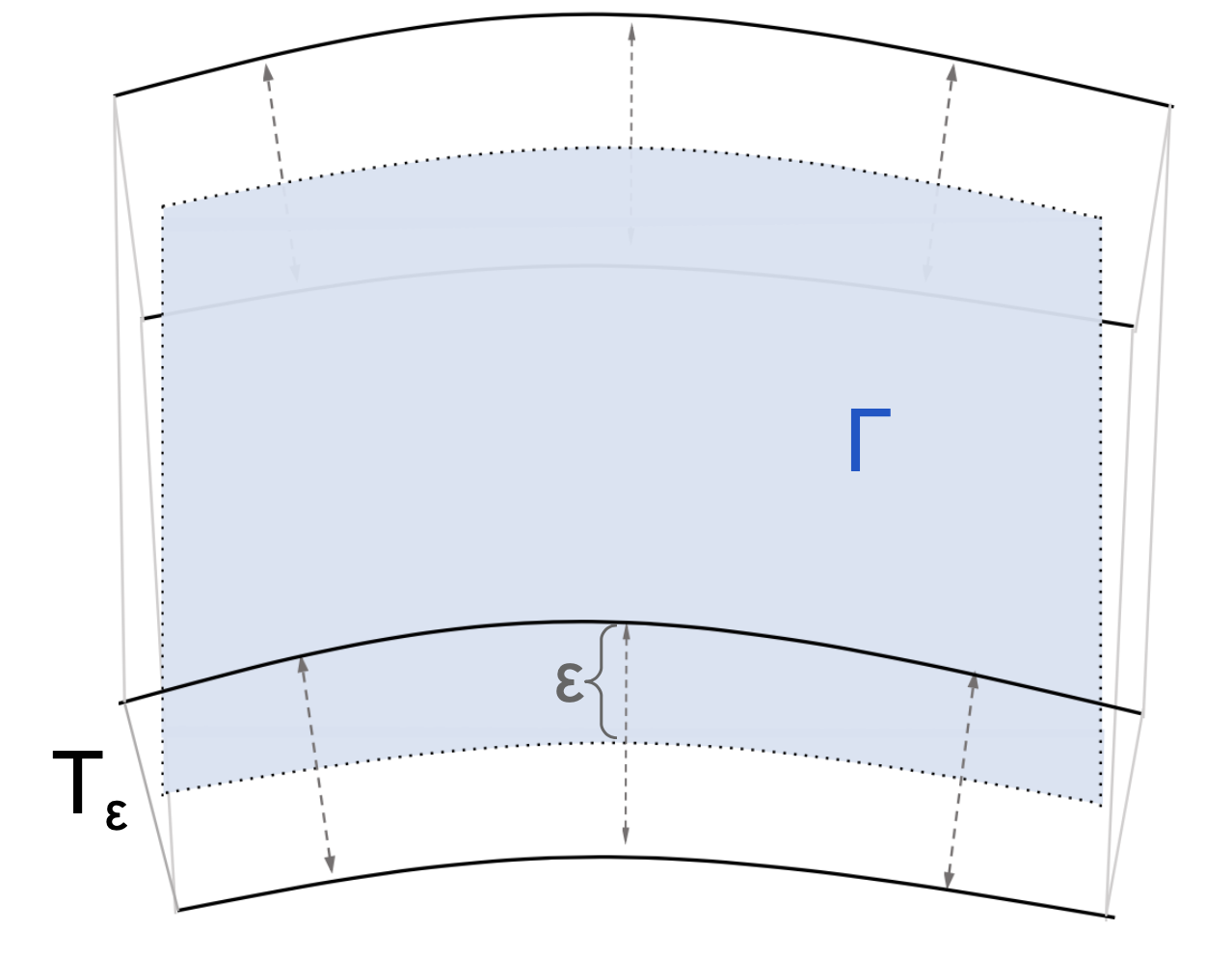
We will work with the tubular neighborhood $T_{\epsilon}\subset\mathbb{R}^{3}$ of $\Gamma$ :

(16)

T_{\epsilon}:=\left\{\mathbf{z}\in\mathbb{R}^{3}:\left\|\mathbf{z}-\mathbf{p}\right\|<\epsilon<\tau_{\Gamma},\mathbf{p}\in\Gamma\right\}.

See Figure 1, for a schematic depiction. In $T_{\epsilon}$ , the closest point mapping to $\Gamma$

(17)

P_{\Gamma}(\mathbf{z}):=\text{argmin}_{\boldsymbol{x}\in\Gamma}||\mathbf{z}-\mathbf{x}||,

and the normal vector field $\mathbf{n}(\mathbf{z}):=\nabla\phi_{\Gamma}(\mathbf{z})$ are well-defined; furthermore,

\mathbf{n}(\mathbf{z})=\mathbf{n}(P_{\Gamma}\mathbf{z})~{}~{}\text{and}~{}~{}\phi_{\Gamma}(\mathbf{z})=\mathbf{n}(\mathbf{z})\cdot(\mathbf{z}-P_{\Gamma}{\mathbf{z}}).

Refer to caption — Figure 1. New Optimal Transport problems are defined in $T_{\epsilon}$ to have solutions to the Optimal Transport problems on $\Gamma$ .

3.2. Extension of Surface Densities

Let $\rho\in\Theta_{\Gamma}$ , we can rewrite the integration of $f$ on $\Gamma$ to one on $\Gamma_{\eta}\subset T_{\epsilon}$ as follows:

(18)

\int_{\Gamma}\rho(\mathbf{x})dS=\int_{\Gamma_{\eta}}\rho(P_{\Gamma}\mathbf{z}^{\prime})J(\mathbf{z}^{\prime})dS,

where $J(\mathbf{z}^{\prime})$ accounts for the change of variables in the integrations. In fact,

(19)

J(\mathbf{z}^{\prime})=(1-\kappa_{1}\phi_{\Gamma})(1-\kappa_{2}\phi_{\Gamma})(\mathbf{z}^{\prime})=\sigma_{1}(\mathbf{z}^{\prime})\sigma_{2}(\mathbf{z}^{\prime}),

where $\kappa_{1},\kappa_{2}$ are the two principal curvatures of $\Gamma_{\eta}$ at $\mathbf{z}^{\prime}$ whose signs are determined by the surface orientation, and $\sigma_{1},\sigma_{2}$ are the two largest singular values of the Jacobian matrix of $P_{\Gamma}$ . See e.g. [29].

Furthermore, by the coarea formula,

\displaystyle 1=\int_{\Gamma}f(\mathbf{x})dS=\frac{1}{2\epsilon}\int_{-\epsilon}^{\epsilon}\int_{\Gamma_{y}}f(P_{\Gamma}\mathbf{z}^{\prime})J(\mathbf{z}^{\prime})dSd\eta

\displaystyle=\frac{1}{2\epsilon}\int_{T_{\epsilon}}f(P_{\Gamma}\mathbf{z})J(\mathbf{z})d\mathbf{z}.

Therefore, our extended Optimal Transport problem is formulated with the class of density function defined below:

(20)

\Theta_{T_{\epsilon}}:=\left\{\frac{1}{2\epsilon}\rho(P_{\Gamma}\mathbf{z})J(\mathbf{z}):\rho\in\Theta_{\Gamma}\right\}.

Therefore, any density in $\Theta_{T_{\epsilon}}$ is strictly positive and smooth (The Jacobian $J$ is smooth and strictly positive since we stay within the reach of $\Gamma$ .)

3.3. Extension of Cost Function to $T_{\epsilon}$

Let $c$ be the cost function defined on $\Gamma$ . We define the extended cost function for any two points in $T_{\epsilon}$ by adding an additional cost to the difference in their distance to $\Gamma$ :

(21)

c_{\sigma}(\mathbf{z}_{1},\mathbf{z}_{2})=c(P_{\Gamma}\mathbf{z}_{1},P_{\Gamma}\mathbf{z}_{2})+\frac{\sigma}{2}(\phi_{\Gamma}(\mathbf{z}_{1})-\phi_{\Gamma}(\mathbf{z}_{2}))^{2},~{}~{}~{}\text{for some}~{}\sigma>0.

We will see that the particular choice of $\sigma$ will not affect the analysis.

3.4. Equivalence of the Two Optimal Transport Problems

In this section, we establish that the Optimal Transport problem defined via our extensions of the density functions and the cost function in Sections 3.2 and 3.3 leads to an Optimal Transport mapping $\overline{\mathbf{m}}$ that moves mass only along each level set of the distance function to $\Gamma$ . Moreover, $\overline{\mathbf{m}}$ can be used to find $\mathbf{m}$ , the mapping from the Optimal Transport problem on $\Gamma$ .

Theorem 4.

The solution, $\overline{\mathbf{m}}$ , to the new Optimal Transport problem presented in Equation (10) defined with the densities in $\Theta_{T_{\epsilon}}$ and cost function in Equation (21), satisfies

(22)

P_{\Gamma}\overline{\mathbf{m}}(\mathbf{z})=\mathbf{m}(P_{\Gamma}\mathbf{z}),~{}~{}~{}\forall\mathbf{z}\in T_{\epsilon},

and

(23)

\phi_{\Gamma}(\mathbf{z})=\phi_{\Gamma}(\overline{\mathbf{m}}(\mathbf{z})),~{}~{}~{}\forall\mathbf{z}\in T_{\epsilon}.

This theorem then implies that the Optimal Transport cost for the Optimal Transport problem on $\Gamma$ is equal to the Optimal Transport cost for the extended Optimal Transport problem on $T_{\epsilon}$ . Thus, the Wasserstein distance, for example, on $\Gamma$ can be computed via the extended Optimal Transport problem on $T_{\epsilon}$ .

Corollary 5.

We have

(24)

\min_{\boldsymbol{\xi}_{\#}\overline{\mu}=\overline{\nu}}\int_{T_{\epsilon}}c_{\sigma}(\mathbf{z},\boldsymbol{\xi}(\mathbf{z}))\overline{f}(\mathbf{z})d\mathbf{z}=\min_{\boldsymbol{\theta}_{\#}\mu=\nu}\int_{\Gamma}c(\mathbf{x},\boldsymbol{\theta}(\mathbf{x}))f(\mathbf{x})dS(\mathbf{x}).

Proof.

	$\displaystyle\min_{\boldsymbol{\xi}_{\#}\overline{\mu}=\overline{\nu}}\int_{T_{\epsilon}}c_{\sigma}(\mathbf{z},\boldsymbol{\xi}(\mathbf{z}))\overline{f}(\mathbf{z})d\mathbf{z}$	$\displaystyle=\int_{T_{\epsilon}}c_{\sigma}(\mathbf{z},\overline{\mathbf{m}}(\mathbf{z}))\overline{f}(\mathbf{z})d\mathbf{z}$
		$\displaystyle=\int_{T_{\epsilon}}c(P_{\Gamma}\mathbf{z},P_{\Gamma}\overline{\mathbf{m}}(\mathbf{z}))\overline{f}(\mathbf{z})d\mathbf{z}$
		$\displaystyle=\frac{1}{2\epsilon}\int_{-\epsilon}^{\epsilon}\int_{\Gamma_{\eta}}c(P_{\Gamma}\mathbf{z},P_{\Gamma}\overline{\mathbf{m}}(\mathbf{z}))f(\mathbf{x})J(\mathbf{z})dS(\mathbf{z})d\eta$
		$\displaystyle=\frac{1}{2\epsilon}\int_{-\epsilon}^{\epsilon}\int_{\Gamma}c(\mathbf{x},\mathbf{m}(\mathbf{x}))f(\mathbf{x})dS(\mathbf{x})d\eta$
		$\displaystyle=\int_{\Gamma}c(\mathbf{x},\mathbf{m}(\mathbf{x}))f(\mathbf{x})dS(\mathbf{x})$
		$\displaystyle=\min_{\boldsymbol{\theta}_{\#}\mu=\nu}\int_{\Gamma}c(\mathbf{x},\boldsymbol{\theta}(\mathbf{x}))f(\mathbf{x})dS(\mathbf{x}).$

∎

Mass preservation

Since $\epsilon<\tau_{\Gamma}$ and $\Gamma$ is compact and closed, the projection $P_{\Gamma}$ is bijective between $\Gamma$ and $\Gamma_{\eta}$ for any $\eta\in(-\epsilon,\epsilon).$ We define the inverse map

(25)

P_{\Gamma,\Gamma_{\eta}}^{-1}(\mathbf{z}):=\mathbf{z}+\eta\mathbf{n}(\mathbf{z}),~{}~{}~{}\text{for}~{}\mathbf{z}\in\Gamma,

where $\mathbf{n}(\mathbf{z})=\nabla\phi_{\Gamma}(\mathbf{z})$ is the outward normal vector of $\Gamma$ at $\mathbf{z}$ . This vector remains the same for all $\mathbf{z}^{\prime}\in T_{\epsilon}$ satisfying $P_{\Gamma}\mathbf{z}^{\prime}=\mathbf{z}.$ Thus we see that $P_{\Gamma}\circ P^{-1}_{\Gamma,\Gamma_{\eta}}(\mathbf{z})=\mathbf{z}$ and $P^{-1}_{\Gamma,\Gamma_{\eta}}\circ P_{\Gamma}(\mathbf{z}^{\prime})=\mathbf{z}^{\prime}$ for $\mathbf{z}^{\prime}\in\Gamma_{\eta}.$ Therefore, we can associate any mapping $\boldsymbol{\xi}:\Gamma\mapsto\Gamma$ with $\boldsymbol{\xi}\circ P_{\Gamma}:\Gamma_{\eta}\mapsto\Gamma_{\eta}$ and vice versa. So we define

(26)

\boldsymbol{\xi}_{\epsilon}(\mathbf{z}):=P_{\Gamma,\Gamma_{\eta}}^{-1}\circ\boldsymbol{\xi}\circ P_{\Gamma}(\mathbf{z}),~{}~{}~{}\phi_{\Gamma}(\mathbf{z})=\eta,~{}~{}\text{and}~{}\eta\in(-\epsilon,\epsilon).

Equivalently,

(27)

P_{\Gamma}\boldsymbol{\xi}_{\epsilon}(\mathbf{z}^{\prime})=\boldsymbol{\xi}(P_{\Gamma}\mathbf{z}^{\prime}),~{}~{}~{}\mathbf{z}\in T_{\epsilon},

and

(28)

\phi_{\Gamma}(\boldsymbol{\xi}_{\epsilon}(\mathbf{z}^{\prime}))=\phi_{\Gamma}(\boldsymbol{\xi}_{\epsilon}(\mathbf{z}^{\prime})),~{}~{}~{}\mathbf{z}\in T_{\epsilon}.

In particular, suppose $\mathbf{m}$ is the solution to the Optimal transport problem in Equation (3) on $\Gamma$ . Then, we will show that

(29)

\tilde{\mathbf{m}}(\mathbf{z}):=(P_{\Gamma}\mathbf{z}+\phi_{\Gamma}(\mathbf{z})\mathbf{n}(\mathbf{z}))~{}\mathbf{m}(P_{\Gamma}\mathbf{z})

is a solution to the extended Optimal Transport problem in Equation (10).

The first step is to show that if $\boldsymbol{\xi}\#\mu=\nu$ with $\mu=fdS$ and $\nu=gdS$ , then $\boldsymbol{\xi}_{\epsilon}\mu=\nu$ , with $\mu=f_{\epsilon}d\mathbf{x}$ , and $\nu=g_{\epsilon}d\mathbf{x}$ . But this is another exercise on the coarea formula. Let $E\subset T_{\epsilon}$ , we have

	$\displaystyle\int_{E}\overline{g}(\mathbf{x})d\mathbf{x}$	$\displaystyle=\int_{-\epsilon}^{\epsilon}\int_{E\cap\Gamma_{\eta}}g(P_{\Gamma}\mathbf{z}^{\prime})J(\mathbf{z}^{\prime})~{}dSd\eta$
		$\displaystyle=\int_{-\epsilon}^{\epsilon}\int_{P_{\Gamma}(E\cap\Gamma_{\eta})}g(\mathbf{z})~{}dSd\eta$
		$\displaystyle=\int_{-\epsilon}^{\epsilon}\int_{\boldsymbol{\xi}^{-1}(P_{\Gamma}(E\cap\Gamma_{\eta}))}f(\mathbf{z})~{}dSd\eta$
		$\displaystyle=\int_{-\epsilon}^{\epsilon}\int_{P^{-1}_{\Gamma,\Gamma_{\eta}}(\boldsymbol{\xi}^{-1}(P_{\Gamma}(E\cap\Gamma_{\eta})))}f(P_{\Gamma}\mathbf{z})J(\mathbf{z})~{}dSd\eta$
		$\displaystyle=\int_{-\epsilon}^{\epsilon}\int_{\boldsymbol{\xi}_{\epsilon}^{-1}(E\cap\Gamma_{\eta})}f(P_{\Gamma}\mathbf{z}^{\prime})J(\mathbf{z}^{\prime})~{}dSd\eta=\int_{\boldsymbol{\xi}_{\epsilon}^{-1}(E)}\overline{f}(\mathbf{x})d\mathbf{x},$

where the penultimate equality follows since $P_{\Gamma,\Gamma_{\eta}}^{-1}\circ\boldsymbol{\xi}^{-1}\circ P_{\Gamma}\circ P^{-1}_{\Gamma,\Gamma_{\eta}}\circ\boldsymbol{\xi}\circ P_{\Gamma}=P_{\Gamma,\Gamma_{\eta}}^{-1}\circ\boldsymbol{\xi}^{-1}\circ\boldsymbol{\xi}\circ P_{\Gamma}=P_{\Gamma,\Gamma_{\eta}}^{-1}\circ P_{\Gamma}=\text{Id}$ , we then know that $P^{-1}_{\Gamma,\Gamma_{\eta}}(\boldsymbol{\xi}^{-1}(P_{\Gamma}(E\cap\Gamma_{\eta})))=\boldsymbol{\xi}_{\epsilon}^{-1}(E\cap\Gamma_{\eta})$ .

Comparing Equation (10) with Equation (21), Equation (18), and Equation (20), we see that the transport cost over all $\boldsymbol{\xi}_{\epsilon}$ is minimized for $\boldsymbol{\xi}_{\epsilon}=\tilde{\mathbf{m}}$ :

(30)			$\displaystyle\int_{T_{\epsilon}}c_{\sigma}\left(\mathbf{z}^{\prime},\boldsymbol{\xi}_{\epsilon}(\mathbf{z}^{\prime})\right)\overline{f}(\mathbf{z}^{\prime})d\mathbf{z}^{\prime}$
			$\displaystyle=\int_{-\epsilon}^{\epsilon}\int_{\Gamma_{\eta}}c(P_{\Gamma}\mathbf{z}^{\prime},P_{\Gamma}\boldsymbol{\xi}_{\epsilon}(\mathbf{z}^{\prime}))f(P_{\Gamma}\mathbf{z}^{\prime})J(\mathbf{z}^{\prime})dSd\eta$
			$\displaystyle=2\epsilon\int_{\Gamma}c(\mathbf{z},\boldsymbol{\xi}(\mathbf{z}))f(\mathbf{z})dS$
			$\displaystyle\geq 2\epsilon\int_{\Gamma}c(\mathbf{z},\boldsymbol{m}(\mathbf{z}))f(\mathbf{z})dS=\int_{T_{\epsilon}}c_{\sigma}\left(\mathbf{z}^{\prime},\tilde{\boldsymbol{m}}_{\epsilon}(\mathbf{z}^{\prime})\right)\overline{f}(\mathbf{z}^{\prime})d\mathbf{z}^{\prime},$

Following the above construction, we see that Equation (22) holds for $\tilde{\mathbf{m}}$ . Now consider $\mathbf{z}_{y}\in\Gamma_{y}$ . By construction, $\tilde{\mathbf{m}}(\mathbf{z}_{y})\in\Gamma_{\eta},$ implying Equation (23). $\tilde{\mathbf{m}}(\mathbf{z})$ does not move mass in the normal direction of $\Gamma$ .

For our extended problem, since the source and target densities are supported on $\mathbb{R}^{3}$ , the Optimal Mapping $\overline{\mathbf{m}}$ and potential function $v$ satisfy:

(31)

\nabla v(\mathbf{z})=-\nabla_{\mathbf{z}}c_{\sigma}(\mathbf{z},\boldsymbol{\xi}),

for $\boldsymbol{\xi}=\overline{\mathbf{m}}(\mathbf{z})$ , where we emphasize that $\nabla$ is the Euclidean gradient and $v$ is $c_{\sigma}$ -convex. The relation defined in Equation (31) applied to $\tilde{\mathbf{m}}$ and separated into one defined on surfaces that are equidistant to $\Gamma$ becomes

(32)

(I-\mathbf{n}\otimes\mathbf{n})\nabla\tilde{v}(\mathbf{z})=-(I-\mathbf{n}\otimes\mathbf{n})\nabla_{\mathbf{z}}c\left(P_{\Gamma}\mathbf{z},\mathbf{m}\right),

and one in the normal direction of the surface,

(33)

\nabla\tilde{v}(\mathbf{z})\cdot\mathbf{n}=\sigma\left(\phi_{\Gamma}(\tilde{\mathbf{m}}(\mathbf{z}))-\phi_{\Gamma}(\mathbf{z})\right).

Here $\mathbf{n}$ is the normal of $\Gamma$ at $P_{\Gamma}\mathbf{z}$ . Notice that for $\mathbf{z}\in\Gamma$ , Equation (32) is Equation (7). This means that the restriction of $v$ on $\Gamma$ solves Equation (7).

Using Equation (23) in Equation (33), we obtain

(34)

\frac{\partial\tilde{v}}{\partial\mathbf{n}}(\mathbf{z})=0,~{}~{}~{}\mathbf{z}\in T_{\epsilon}.

Then, by Equation (32)

\tilde{v}(\mathbf{z})=u(P_{\Gamma}\mathbf{z})+C,

for some constant $C$ and $P_{\Gamma}\overline{\mathbf{m}}(\mathbf{z})=\mathbf{m}(P_{\Gamma}\mathbf{z})$ , which is the solution pair from the Optimal Transport problem on $\Gamma$ .

Now, in order to finish the proof of Theorem 4, it remains to show that $\tilde{v}$ is $\bar{c}$ -convex. Once this is shown, then by Theorem 3 there is a unique solution of the Optimal Transport problem in Equation (10), then we have shown, in fact, $\tilde{\mathbf{m}}=\overline{\mathbf{m}}$ satisfying $\phi_{\Gamma}(\overline{\mathbf{m}}(\mathbf{z}))=\phi_{\Gamma}(\mathbf{z})$ and $P_{\Gamma}\overline{\mathbf{m}}(\mathbf{z})=\mathbf{m}(P_{\Gamma}\mathbf{z})$ .

$c_{\sigma}$ -Convexity of the Potential Function

Lemma 6.

$\tilde{v}(\mathbf{z})=u(P_{\Gamma}\mathbf{z})$ is $\bar{c}$ -convex.

Proof.

Recall the definition of $c$ -convexity from Definition 2: $u$ is $c$ -convex since it is the potential function for the Optimal Transport problem on $\Gamma$ . This means that for all $\mathbf{x}\in\Gamma$ , there exists a point $\mathbf{\tilde{x}}\in\Gamma$ and the $c$ -transform of $u$ satisfies $u^{c}(\mathbf{\tilde{x}})$ such that:

(35)		$\displaystyle-u^{c}(\mathbf{\tilde{x}})-c(\mathbf{x},\mathbf{\tilde{x}})$	$\displaystyle=u(\mathbf{x}),$
(36)		$\displaystyle-u^{c}(\mathbf{\tilde{x}})-c(\mathbf{x}^{\prime},\mathbf{\tilde{x}})$	$\displaystyle\leq u(\mathbf{x}^{\prime}),\ \forall\mathbf{x}^{\prime}\in\Gamma.$

Now, fix $\mathbf{x}\in\Gamma$ and fix a $\mathbf{z}\in T_{\epsilon}$ such that $P_{\Gamma}\mathbf{z}=\mathbf{x}$ . From Equation (35), given $\mathbf{x}\in\Gamma$ , we have an $\tilde{\mathbf{x}}\in\Gamma$ such that Equation (35) holds. Choose $\tilde{\mathbf{z}}$ such that $P_{\Gamma}\tilde{\mathbf{x}}=\tilde{\mathbf{x}}$ and $\phi_{\Gamma}\tilde{\mathbf{z}}=\phi_{\Gamma}\mathbf{z}$ . By the definition of the $c_{\sigma}$ -transform in $T_{\epsilon}$ :

(37)

\tilde{v}^{c_{\sigma}}(\mathbf{\tilde{z}})=\sup_{\boldsymbol{\xi}}\left(-c_{\sigma}(\boldsymbol{\xi},\mathbf{\tilde{z}})-\tilde{v}(\boldsymbol{\xi})-C\right),

(38)

=\sup_{P_{\Gamma}\boldsymbol{\xi,\phi_{\Gamma}\boldsymbol{\xi}}}\left(-c(P_{\Gamma}\boldsymbol{\xi},\mathbf{\tilde{x}})-\frac{\sigma}{2}(\phi_{\Gamma}\boldsymbol{\xi}-\phi_{\Gamma}\tilde{\mathbf{z}})^{2}-u(P_{\Gamma}\boldsymbol{\xi})-C\right),

we can immediately take the supremum over $\phi_{\Gamma}\boldsymbol{\xi}$ by choosing $\phi_{\Gamma}\boldsymbol{\xi}=\phi_{\Gamma}\tilde{\mathbf{z}}$ , since the other terms do not depend on $\phi_{\Gamma}\boldsymbol{\xi}$ . Thus,

(39)

\tilde{v}^{c_{\sigma}}(\mathbf{\tilde{z}})=\sup_{P_{\Gamma}\boldsymbol{\xi}}\left(-c(P_{\Gamma}\boldsymbol{\xi},\mathbf{\tilde{x}})-u(P_{\Gamma}\boldsymbol{\xi})-C\right)=u^{c}(\mathbf{\tilde{x}})-C.

Thus, we get:

(40)

-\tilde{v}^{c_{\sigma}}(\mathbf{\tilde{z}})-c_{\sigma}(\mathbf{z},\mathbf{\tilde{z}})=-u^{c}(\mathbf{\tilde{x}})+C-c(P_{\Gamma}\mathbf{z},\mathbf{\tilde{x}})=u(P_{\Gamma}\mathbf{z})+C=\tilde{v}(\mathbf{z}),

by Equation (35). Now, for any $\mathbf{z}^{\prime}\in T_{\epsilon}$ . Then,

(41)

-\tilde{v}^{c_{\sigma}}(\mathbf{\tilde{z}})-c_{\sigma}(\mathbf{z}^{\prime},\mathbf{\tilde{z}})=-u^{c}(\mathbf{\tilde{x}})+C-\frac{\sigma}{2}(\phi_{\Gamma}\mathbf{z}^{\prime}-\phi_{\Gamma}\tilde{\mathbf{z}})^{2}-c(P_{\Gamma}\mathbf{z}^{\prime},P_{\Gamma}\tilde{\mathbf{z}})\leq\\ -u^{c}(\mathbf{\tilde{x}})+C-c(P_{\Gamma}\mathbf{z}^{\prime},P_{\Gamma}\tilde{\mathbf{z}})\leq u(P_{\Gamma}\mathbf{z}^{\prime})+C=\tilde{v}(\mathbf{z}^{\prime}),\ \forall\mathbf{z}^{\prime},

by Equation (36). Thus, $\tilde{v}$ is $c_{\sigma}$ -convex.

∎

3.5. Example: Optimal Transport on the Unit Sphere

In our numerical implementation in Section 4, we have found it fruitful to utilize explicit expressions for the Optimal Transport mapping in terms of the Euclidean gradient of the potential function. We have also found it useful on the sphere to simply use explicit expressions for the mixed Hessian terms in the PDE (11). Expressions for the mixed Hessian are much more difficult to derive on other surfaces, so in those cases the simple discretization presented in Section 4 is used instead. In practice, it is perfectly reasonable to eschew these analytical derivations and simply discretize the PDE system (11) directly.

Let $\Gamma$ be the unit sphere in $\mathbb{R}^{3}$ . Although we will be using the usual spherical polar coordinates, $\mathbf{z}=(r\cos\phi\sin\theta,r\sin\phi\sin\theta,r\cos\theta),$ for $0\leq\phi<2\pi$ , $0\leq\theta\leq\pi$ , on the sphere we will not need to derive many quantities that depend on the coordinates $\theta$ and $\phi$ . One minor exception is the surface area element $dS=r\sin(\theta)d\phi d\theta$ which will be useful for integrating the source and target densities $f$ and $g$ when they are explicitly known. Some of the important quantities that do not depend on $\theta$ and $\phi$ are:

\phi_{\Gamma}(\mathbf{z})=r-1,~{}P_{\Gamma}\mathbf{z}=\frac{\mathbf{z}}{||\mathbf{z}||},~{}J(\mathbf{z})=1-\frac{\phi_{\Gamma}(\mathbf{z})}{1+\phi_{\Gamma}(\mathbf{z})}=\frac{1}{r^{2}}.

Thus densities in $\Theta_{T_{\epsilon}}$ take the form

\overline{\rho}(r,\phi,\theta)=\frac{\rho(\phi,\theta)}{2\epsilon r^{2}}.

Case 1: $c(\mathbf{x},\mathbf{y})=\frac{1}{2}d_{\mathbb{S}^{2}}(\mathbf{x},\mathbf{y})$ is the the squared geodesic distance between $\mathbf{x}$ and $\mathbf{y}$ on the unit sphere.

The extended cost function on the unit sphere has the explicit form $c(\mathbf{x},\mathbf{y})=\frac{1}{2}\arccos(\mathbf{x}\cdot\mathbf{y})^{2}$ , and consequently we have:

(42)

c_{\sigma}(\mathbf{z},\boldsymbol{\xi})=\frac{\sigma}{2}\left(||\mathbf{z}||-||\boldsymbol{\xi}||\right)^{2}+\frac{1}{2}\arccos\left(\frac{\mathbf{z}}{||\mathbf{z}||}\cdot\frac{\boldsymbol{\xi}}{||\boldsymbol{\xi}||}\right)^{2},

Once we have chosen a cost function, we can compute the Optimal Transport mapping. The Optimal Transport mapping $\overline{\mathbf{m}}(\mathbf{z})$ can be found by solving Equations (32)and (33). Thus, we find:

(43)

\phi_{\Gamma}(\overline{\mathbf{m}}(\mathbf{z}))=\phi_{\Gamma}(\mathbf{z})+\frac{1}{\sigma}\nabla v(\mathbf{z})\cdot\mathbf{n},

and

(44)

P_{\Gamma}(\overline{\mathbf{m}}(\mathbf{z}))=\text{exp}_{P_{\Gamma}(\mathbf{z})}\left((1+\phi_{\Gamma}(\mathbf{z}))\left(I-\mathbf{n}\otimes\mathbf{n}\right)\nabla v(\mathbf{z})\right),

which states that the projection of $\nabla v$ onto the tangent plane is multiplied by the factor $1+\phi_{\Gamma}(\mathbf{z})$ and then transported via the exponential map on $\mathbb{S}^{2}$ starting at the point $P_{\Gamma}(\mathbf{z})$ in the direction of the projection of $\nabla v$ onto the tangent plane at $P_{\Gamma}(\mathbf{z})$ . This leads to the expression:

(45)

\overline{\mathbf{m}}(\mathbf{z})=P_{\Gamma}(\overline{\mathbf{m}}(\mathbf{z}))+\phi_{\Gamma}\left(\overline{\mathbf{m}}(\mathbf{z})\right)\mathbf{n}.

The mixed Hessian term in $T_{\epsilon}$ can be derived by using the mixed Hessian term for the squared geodesic cost on the unit sphere [22], [23]:

(46)

\left|\det D^{2}_{\mathbf{x}\mathbf{y},\mathbb{S}^{2}}\left(\frac{1}{2}d_{\mathbb{S}^{2}}(\mathbf{x},\mathbf{y})^{2}\right)\right|=\frac{\left\|\nabla_{\mathbb{S}^{2}}u(\mathbf{x})\right\|}{\sin\left(\left\|\nabla_{\mathbb{S}^{2}}u(\mathbf{x})\right\|\right)}.

Denoting $\nabla_{\Gamma_{\eta}}v(\mathbf{z})=(I-\mathbf{n}\otimes\mathbf{n})\nabla v(\mathbf{z})$ , the corresponding mixed Hessian for the extended problem is:

(47)

\left|\det D^{2}_{\mathbf{z}\boldsymbol{\xi}}c_{\sigma}(\mathbf{z},\boldsymbol{\xi})\right|=\sigma\frac{\left\|(1+\phi_{\Gamma}(\mathbf{z}))\nabla_{\Gamma_{\eta}}v(\mathbf{z})\right\|}{(1+\phi_{\Gamma}(\mathbf{z}))^{2}\sin\left(\left\|(1+\phi_{\Gamma}(\mathbf{z}))\nabla_{\Gamma_{\eta}}v(\mathbf{z})\right\|\right)},

for $\boldsymbol{\xi}=\overline{\mathbf{m}}(\mathbf{z})=\mathbf{m}(P_{\Gamma}\mathbf{z})$ .

Case 2: $c(\mathbf{x},\mathbf{y})=-\log(1-\mathbf{x}\cdot\mathbf{y})$ , the logarithmic cost function appearing in the reflector antenna problem.

We have

(48)

c_{\sigma}(\mathbf{z},\boldsymbol{\xi})=\frac{\sigma}{2}\left(||\mathbf{z}||-||\boldsymbol{\xi}||\right)^{2}-\log\left(1-\frac{\mathbf{z}}{||\mathbf{z}||}\cdot\frac{\boldsymbol{\xi}}{||\boldsymbol{\xi}||}\right)^{2}.

The Optimal Transport mapping $\overline{\mathbf{m}}(\mathbf{z})$ can be found by solving Equations (32)and (33). As in the squared geodesic cost case, we find:

(49)

\phi_{\Gamma}(\overline{\mathbf{m}}(\mathbf{z}))=\phi_{\Gamma}(\mathbf{z})+\frac{1}{\sigma}\nabla v(\mathbf{z})\cdot\mathbf{n},

and the optimal transport mapping satisfies [23]:

(50)

P_{\Gamma}\left(\overline{\mathbf{m}}(\mathbf{z})\right)=P_{\Gamma}\mathbf{z}\frac{\left\|(1+\phi_{\Gamma}(\mathbf{z}))\nabla_{\Gamma_{\eta}}v(\mathbf{z})\right\|^{2}-1}{\left\|(1+\phi_{\Gamma}(\mathbf{z}))\nabla_{\Gamma_{\eta}}v(\mathbf{z})\right\|^{2}+1}\\ -(1+\phi_{\Gamma}(\mathbf{z}))\nabla_{\Gamma_{\eta}}v(\mathbf{z})\frac{2}{\left\|(1+\phi_{\Gamma}(\mathbf{z}))\nabla_{\Gamma_{\eta}}v(\mathbf{z})\right\|^{2}+1}.

As with the squared geodesic cost function, this leads to the expression:

(51)

\overline{\mathbf{m}}(\mathbf{z})=P_{\Gamma}(\overline{\mathbf{m}}(\mathbf{z}))+\phi_{\Gamma}\left(\overline{\mathbf{m}}(\mathbf{z})\right)\mathbf{n}.

In this case, the mixed Hessian term for the logarithmic cost on the sphere is:

(52)

\left|\det D^{2}_{\mathbf{x}\mathbf{y},\mathbb{S}^{2}}\left(-\log(1-\mathbf{x}\cdot\mathbf{y})\right)\right|=\frac{\left(\left\|\nabla_{\mathbb{S}^{2}}u(\mathbf{x})\right\|^{2}+1\right)^{2}}{4},

for $\boldsymbol{\xi}=\overline{\mathbf{m}}(\mathbf{z})$ . The corresponding mixed Hessian for the extended problem on $T_{\epsilon}$ is:

(53)

\left|\det D^{2}_{\mathbf{z}\boldsymbol{\xi}}c_{\sigma}(\mathbf{z},\boldsymbol{\xi})\right|=\frac{\sigma\left(\left\|(1+\phi_{\Gamma}(\mathbf{z}))\nabla_{\Gamma_{\eta}}v(\mathbf{z})\right\|^{2}+1\right)^{2}}{4(1+\phi_{\Gamma}(\mathbf{z}))^{2}},

for $\boldsymbol{\xi}=\overline{\mathbf{m}}(\mathbf{z})$ .

3.6. Optimal Transport on Surfaces with Boundary

Here we outline how the proposed volumetric approach may be generalized to surfaces with smooth boundaries. Let $\Gamma$ be the boundary of a subset $\Omega\subset\mathbb{R}^{3}$ . Let $\Gamma_{1}$ and $\Gamma_{2}$ be two open subsets of $\Gamma$ such that $\partial\Gamma_{1}=\partial\Gamma_{2}$ is a closed smooth curve and

\Gamma=\overline{\Gamma_{1}\cup\Gamma_{2}}.

Take $\Gamma$ for a sphere for instance, $\Gamma_{1}$ and $\Gamma_{2}$ can be respectively the northern and the southern hemisphere, and $\partial\Gamma_{1}=\partial\Gamma_{2}$ is the equator.

Consider the following partitioning of $T_{\epsilon}$ :

T_{\epsilon}:=\{\mathbf{x}\in\mathbb{R}^{3}:\min_{\mathbf{z}\in\Gamma_{1}}|\mathbf{x}-\mathbf{z}|<\epsilon\}=T_{\epsilon}^{1}\cup Q_{\epsilon},

where

Q_{\epsilon}=\{\mathbf{z}\in T_{\epsilon}:P_{\Gamma}\mathbf{z}\in\partial\Gamma_{1}\}.

Starting from the optimization problem involving the source and target densities $f,g:\Gamma_{1}\mapsto\mathbb{R}$ satisfying

\text{supp}(f)\subseteq\text{supp}(g)=\Gamma_{1},

we will formally arrive at the same optimal transport PDEs defined in (11), but posed in $T_{\epsilon}^{1}$ instead of $T_{\epsilon}$ , and with zero Neumann boundary imposed on $\partial T_{\epsilon}^{1}$ . Notice that the essential ingredients used in the extension, $P_{\Gamma_{1}}\equiv P_{\Gamma}$ and $J_{\Gamma_{1}}\equiv J_{\Gamma}$ in $T_{\epsilon}^{1}$ , so the extended optimal transport problem can be defined without further complication.

Following the theory developed in [55][20], we will then impose the zero Neumann condition on $\partial T_{\epsilon}^{1}$ . Of course on $\partial T^{1}_{\epsilon}\cap\partial T_{\epsilon}$ , we can apply a similar procedure described in (61). On the face $\partial T^{1}_{\epsilon}\cap\partial Q_{\epsilon}$ , we can adopt the standard finite difference approach to enforce Neumann condition; e.g. [6, 25].

4. Computational Examples

The key innovation in reformulating the Optimal Transport problem of $\Gamma$ to one on $T_{\epsilon}$ is to allow for a wide selection of numerical discretizations for the PDE (11) defined on $T_{\epsilon}$ . In this section, we present a simple method using uniform Cartesian grids and demonstrate some computational results using the method.

We will discretize (11) and compute most of the needed geometric information about $\Gamma$ on the part of a uniform Cartesian grid lying within

\mathcal{T}_{\epsilon}^{h}=h\mathbb{Z}^{3}\cap T_{\epsilon},

which will consist of interior points, where we perform a full PDE solve using the PDE (11) and boundary points, where we exploit the fact that the potential function is a priori known to be constant in the normal direction.

The grid is assumed to resolve the geometry of $\Gamma$ , meaning that the spacing $h$ is smaller than the reach of $\Gamma$ . We will solve the discretized system by the following iterative scheme: for all $\mathbf{z}\in\mathcal{T}_{\epsilon}^{h}$ ,

(54)		$\displaystyle v^{n}_{E}(\mathbf{z})$	$\displaystyle:=v^{n}(\mathbf{z})+\gamma_{n}\left(v^{n}(\mathbf{z})-v^{n-1}(\mathbf{z})\right),$
(54)		$\displaystyle v^{n+1}(\mathbf{z})$	$\displaystyle:=v^{n}_{E}-\Delta tF_{h}(v^{n}_{E},\mathbf{z},\mathcal{N}_{h}(\mathbf{z}));$

Here $F_{h}$ is a finite difference discretization of (11)-(12) and $\mathcal{N}_{h}(\mathbf{z})$ is the set of grid nodes around $\mathbf{z}$ forming the finite difference stencil for the discretization, and $\gamma_{n}$ are small positive numbers, chosen to accelerate the scheme. In Section 4.1 and Section 4.2, we will describe the ingredients in $G_{h}$ used in the numerical experiments in detail.

We will be demonstrating some computational results for the unit sphere, the northern hemisphere of the unit sphere, and for a $2$ -torus in $\mathbb{R}^{3}$ . On the unit sphere, we will employ the squared geodesic cost function $c(\mathbf{x},\mathbf{y})=\frac{1}{2}d_{\mathbb{S}^{2}}(\mathbf{x},\mathbf{y})^{2}$ as well as the logarithmic cost function $c(\mathbf{x},\mathbf{y})=-\log(1-\mathbf{x}\cdot\mathbf{y})$ arising in the reflector antenna problem, see [56, 57]. To make the reflector antenna computation more physically realistic, we also perform a computation on the northern hemisphere of the unit sphere using the logarithmic cost function. Finally, to demonstrate the versatility of the extension method over other surfaces, we perform a computation on a torus $\Gamma\subset\mathbb{R}^{3}$ using the Euclidean cost $c(x,y)=\frac{1}{2}\left\|x-y\right\|^{2}$ on the base manifold $\Gamma$ . We stress here that we do not use the standard Euclidean cost in $\mathbb{R}^{3}$ , but construct the full extended cost $c_{\sigma}$ using $c(x,y)=\frac{1}{2}\left\|x-y\right\|^{2}$ defined for $x,y\in\Gamma$ and add the $\sigma$ -penalty term as explained in Section 3.3.

4.1. Geometry processing

For surfaces defined by level set functions, the computation of the closest point mapping $P_{\Gamma}$ can be done via standard level set methods, see [2, 12, 50, 62]. For surfaces defined by parametrized patches, methods such as those developed in [52] can be used in combination with a KD-tree. As shown in [13], the quantity $J(z)=\sigma_{1}(z)\sigma_{2}(z)$ , where $\sigma_{1}$ and $\sigma_{2}$ are the two largest singular values of $DP_{\Gamma}$ , which can be computed using finite differences.

We recognize that, in contrast to working directly with parameterized surfaces, the reach of $\Gamma$ imposes an important limitation to the mesh size used to discretize $T_{\epsilon},$ independent of the smoothness of the quantities that we wish to compute in $T_{\epsilon}.$ One may resort to adaptive meshing techniques, e.g. [39, 40], for surfaces with small reach.

4.2. Discretization of the PDEs

For any function $f:T_{\epsilon}\rightarrow\mathbb{R}$ , we use the following standard centered-difference discretization $\mathcal{D}^{h}_{1}f(\mathbf{x}_{i})$ , $\mathcal{D}^{h}_{2}f(\mathbf{x}_{i})$ , and $\mathcal{D}^{h}_{3}f(\mathbf{x}_{i})$ for the first-order derivatives $f_{x},f_{y},f_{z}$ at a point $\mathbf{x}_{i}$ , respectively. Letting $\mathbf{e}_{1},\mathbf{e}_{2},\mathbf{e}_{3}$ denote $(1,0,0),(0,1,0)$ , and $(0,0,1)$ , respectively, we compute our first-order derivatives as follows:

\mathcal{D}^{h}_{j}f(\mathbf{x}_{i})=\frac{f(\mathbf{x}_{i}+h\mathbf{e}_{j})-f(\mathbf{x}_{i}-h\mathbf{e}_{j})}{2h}.

Correspondingly, $\nabla f$ is approximated by

(55)

\nabla^{h}f(\mathbf{x}_{i})=\mathcal{D}^{h}_{1}f(\mathbf{x}_{i})\mathbf{e}_{1}+\mathcal{D}^{h}_{2}f(\mathbf{x}_{i})\mathbf{e}_{2}+\mathcal{D}^{h}_{3}f(\mathbf{x}_{i})\mathbf{e}_{3}.

The second-order derivatives are computed by:

\mathcal{D}^{h}_{jj}f(\mathbf{x}_{i})=\frac{f(\mathbf{x}_{i}+h\mathbf{e}_{j})-2f(\mathbf{x}_{i})+f(\mathbf{x}_{i}-h\mathbf{e}_{j})}{h^{2}},

and the following discretization for mixed second-order derivatives:

\mathcal{D}^{h}_{jk}f(\mathbf{x}_{i})=\frac{f(\mathbf{x}_{i}+h(\mathbf{e}_{j}+\mathbf{e}_{k}))+f(\mathbf{x}_{i}-h(\mathbf{e}_{j}+\mathbf{e}_{k}))}{h^{2}}-\\ \frac{f(\mathbf{x}_{i}+h(-\mathbf{e}_{j}+\mathbf{e}_{k}))+f(\mathbf{x}_{i}+h(\mathbf{e}_{j}-\mathbf{e}_{k}))}{h^{2}}.

These second-order derivatives are used in the computation of terms in the determinant of a Hessian matrix:

\det D^{2}F=F_{xx}\left(F_{yy}F_{zz}-F_{yz}^{2}\right)-F_{xy}\left(F_{xy}F_{zz}-F_{xz}F_{yz}\right)+F_{xz}\left(F_{xy}F_{yz}-F_{xz}F_{yy}\right).

We will use $\det D^{2}_{h}F(\mathbf{z})$ to denote the resulting finite difference approximation of $\det D^{2}F(\mathbf{z})$ .

These finite differences collectively define the computational neighborhood $\mathcal{N}^{h}(\mathbf{x}_{i})$ for each grid node $\mathbf{x}_{i}\in\mathcal{T}_{\epsilon}^{h}$ . Hence $\mathcal{N}^{h}(\mathbf{x}_{i})$ contains $18$ grid nodes which are no more than a distance $\sqrt{2}h$ from $\mathbf{x}_{i}$ .

The system of PDEs (11) represents four equations in four unknowns: $v$ , and the coordinates of $\overline{\mathbf{m}}$ . A first possible method would be direct discretization of these four equations. However, since we will be able to solve for the Optimal Transport mapping in terms of the potential function on the base manifold, we opt for the expedient of simply devising a numerical discretization of the first equation in the system of PDEs (11) and deriving an approximation of the mapping which is inspired by Theorem 4. More specifically, we assume that for the given surface $\Gamma$ and cost function $c$ , we can solve for the mapping on the base manifold in terms of the potential function on the base manifold in Equation (9). Then, for our discretization of the PDE system (11), we will simply employ Equation (22) to construct the tangential coordinate of the mapping, by using interpolated values of the discrete gradient of the potential function on the base manifold, and then account for how far the mapping goes in the normal direction via the normal derivative using Equation (33).

From Equation (9), let $\boldsymbol{\alpha}$ denote the map that satisfies $\mathbf{m}=\boldsymbol{\alpha}(\mathbf{p})$ , where $\mathbf{p}=\nabla_{\Gamma}u(\mathbf{x})$ . That is, suppose for any desired cost function on $\Gamma$ , we have analytically derived an expression for the Optimal Transport mapping $\mathbf{m}$ on $\Gamma$ as a function of the gradient of the potential function $\nabla u(\mathbf{x})$ on $\Gamma$ .

We introduce a trilinear interpolation operator $\mathcal{I}_{h}$ : $\mathcal{I}_{h}[v(\mathbf{z})]$ denotes the interpolated values of $v$ at the point $\mathbf{z}\in\Gamma$ using the grid nodes surrounding $\mathbf{z}$ . Of course, if $\mathbf{z}$ is on a grid node, no interpolation is needed. We will be first using the trilinear operator to approximate the Optimal Transport mapping by performing a trilinear interpolation of the projection of the gradient on a local tangent plane computed at the point $P_{\Gamma}\mathbf{x}_{i}$ and then solving Equation (32) for the mapping, for which we assume that we have analytical expressions.

The projection of the finite difference gradient in the normal direction is obtained via the equation

(56)

\mathcal{D}_{\mathbf{n}}^{h}v(\mathbf{x}_{i}):=\left(\nabla^{h}v\cdot\mathbf{n}(\mathbf{x}_{i})\right)\mathbf{n}(\mathbf{x}_{i})\equiv\mathbf{n}\otimes\mathbf{n}(\mathbf{x}_{i})\nabla^{h}v(\mathbf{x}_{i})

and the projection of the gradient onto the local tangent plane via

(57)

\mathcal{D}_{\mathbf{n}^{\perp}}^{h}v(\mathbf{x}_{i})=\left(I-\mathbf{n}\otimes\mathbf{n}(\mathbf{x})\right)\nabla^{h}v(\mathbf{x})

Then, we will compute the following interpolation of the gradient:

(58)

\overline{\mathcal{D}}^{h}_{\mathbf{n}^{\perp}}v(\mathbf{x}_{i}):=\mathcal{I}_{h}\left[\mathcal{D}^{h}_{\mathbf{n}^{\perp}}v(P_{\Gamma}\mathbf{x}_{i})\right].

We then define the approximation of the Optimal Transport mapping on $\mathcal{T}_{\epsilon}^{h}$ as follows:

(59)

\mathbf{m}^{h}(\mathbf{x}_{i}):=\boldsymbol{\alpha}\left(\overline{\mathcal{D}}^{h}_{\mathbf{n}^{\perp}}v(\mathbf{x}_{i})\right)+\mathbf{n}\left(\boldsymbol{\alpha}\left(\overline{\mathcal{D}}^{h}_{\mathbf{n}^{\perp}}v(\mathbf{x}_{i})\right)\right)\left(\phi(\mathbf{x}_{i})+\frac{\nabla^{h}v(\mathbf{x}_{i})\cdot\mathbf{n}(\mathbf{x}_{i})}{\sigma}\right),

which is constructed so that in the tangential coordinates the mapping is approximated by the Optimal Transport mapping on $\Gamma$ and in the normal coordinates, the mapping simply changes by the normal derivative of the potential function divided by $\sigma$ .

Now that we have an approximation of the Optimal Transport mapping, the remainder of the discretization is rather simple. We exploit the fact that in Euclidean space, for all the cost functions $c_{\sigma}(\mathbf{z}_{1},\mathbf{z}_{2})$ considered in this manuscript, a Euclidean derivative with respect to $\mathbf{z}_{1}$ is the same as a Euclidean derivative with respect to $\mathbf{z}_{2}$ , with a minus sign.

In this way, we can fully discretize the PDE (11) on $\mathcal{T}_{\epsilon}^{h}$ . For a point $\mathbf{z}^{\prime}\in T_{\epsilon}$ , define

U_{\mathbf{\mathbf{z}^{\prime}}}(\mathbf{z}):=v(\mathbf{z})+c_{\sigma}(\mathbf{z},\mathbf{z}^{\prime}),

and

(60)

F^{h}_{0}(v(\mathbf{x}_{i})):=\det D^{2}_{h}U_{\mathbf{m}(\mathbf{x}_{i})}(\mathbf{x}_{i})-\left|\det D^{2}_{h}c_{\sigma}(\mathbf{x}_{i},\mathbf{m}(\mathbf{x}_{i}))\right|f(\mathbf{x}_{i})/g(\mathbf{m}(\mathbf{x}_{i})).

The finite dimensional system of equations defined above is not closed, because parts of the finite difference stencil for those grid nodes close to $\partial T_{\epsilon}$ may lie outside of $T_{\epsilon}$ .

Definition 7.

Let $\mathbf{x}_{i}\in h\mathbb{Z}^{3}$ , $\mathcal{N}_{h}(\mathbf{x}_{i})\subset h\mathbb{Z}^{3}$ denotes the set of grid nodes in the finite difference stencil used above. Points in

\mathcal{B}_{h}:=\{\mathbf{y}_{j}\in\mathcal{N}_{h}(\mathbf{x}_{i}):\mathbf{x}_{i}\in T_{\epsilon}\cap h\mathbb{Z}^{3},\mathbf{y}_{j}\notin T_{\epsilon}\}

are called boundary points.

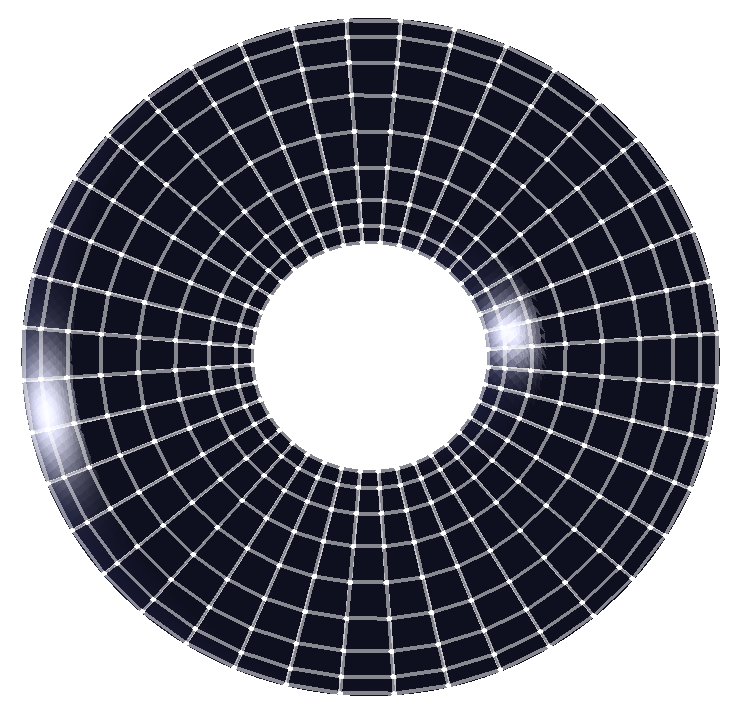
A two-dimensional schematic showing how the computational grid is chosen, as well as a cross-section of computational points showing the boundary points and interior points, is shown in Figure 3.

To obtained a closed system of equations, we will apply suitable closure to the nodes in $\mathcal{B}_{h}$ . The closure condition need to be consistent to the boundary condition in Equation (12). Since the solution $v$ of Equation (11) is a priori constant in the normal direction, we elect to enforce the condition

(61)

v(\mathbf{y}_{j}):=\mathcal{I}_{h}[v(P_{\Gamma}\mathbf{y}_{j})],~{}~{}~{}\mathbf{y}_{j}\in\mathcal{N}_{h}(\mathbf{x}_{i})\cap\mathcal{B}_{h}.

We choose to solve the discrete system (60)-(61) via Algorithm 1. It can be regarded as an accelerated gradient descent method as proposed in [49], where we perform extrapolation with the choice of $\gamma(n)=n/(n+n_{0})$ , for $n_{0}\geq 10$ , as advocated. In practice, we observed that Algorithm 1 without acceleration (setting $\gamma(n)=0$ ) is much less efficient.

The iterations in Algorithm 1 terminate when the residual reaches a value below a desired tolerance. As can be seen from Equation (11), the solution $v$ is unique up to a constant, since the PDE just depends on the derivatives of $v$ . To settle the constant, once the iterations in either Algorithm 1 terminate, we find the minimum value of $u^{h}_{K}$ and define $v$ as $u^{h}_{K}$ minus this minimum value. Thus, the output of the computations is a grid function $v$ whose minimum value is zero.

Algorithm 1 Jacobi-Type Iteration Update with Acceleration

1:Given

v^{h}_{0}

\mathcal{T}^{h}_{\epsilon}

\Delta t>0

\text{tol}>0

v^{h}_{1}(\mathbf{y}_{j}):=\mathcal{I}_{h}[v^{h}_{1}(P_{\Gamma}\mathbf{y}_{j})],~{}~{}~{}\mathbf{y}_{j}\in\mathcal{B}_{h}

v^{h}_{1}(\mathbf{x}_{i}):=v^{h}_{0}(\mathbf{x}_{i})+\Delta tF^{h}_{0}\left(v^{h}_{0}(\mathbf{x}_{i})\right),~{}\forall\mathbf{x}_{i}\in T_{\epsilon}\cap h\mathbb{Z}^{3}

4:Set

n=1

5:while

\max_{\mathbf{x}_{i}\in T_{\epsilon}\cap h\mathbb{Z}^{3}}\left|F^{h}_{0}\left(v^{h}_{n}(\mathbf{x}_{i})\right)\right|>\text{tol}

\forall\mathbf{x}_{i}\in T_{\epsilon}\cap h\mathbb{Z}^{3},

v^{h}_{n,E}(\mathbf{x}_{i}):=v^{h}_{n}(\mathbf{x}_{i})+\gamma(n)(v^{h}_{n}(\mathbf{x}_{i})-v^{h}_{n-1}(\mathbf{x}_{i})))

, for all

\mathbf{x}_{i}\in T_{\epsilon}\cap h\mathbb{Z}^{3}

v^{h}_{n,E}(\mathbf{y}_{j}):=\mathcal{I}_{h}[v^{h}_{n,E}(P_{\Gamma}\mathbf{y}_{j})],~{}~{}~{}\mathbf{y}_{j}\in\mathcal{B}_{h}

v^{h}_{n+1}(\mathbf{x}_{i}):=v^{h}_{n,E}(\mathbf{x}_{i})+\Delta tF^{h}_{0}(v^{h}_{n,E}(\mathbf{x}_{i}))

10:

n:=n+1

11:end while

12:Define

v(\mathbf{x}_{i})=v^{h}(\mathbf{x}_{i})-\min_{i\in\mathcal{T}^{h}_{\epsilon}}v^{h}_{K}(\mathbf{x}_{i})

Remark.

Monotone finite difference schemes are used for discretizing fully nonlinear elliptic PDEs to build convergence guarantees of the discrete solutions even in cases where the solution $v$ is only known to be a priori continuous. There is a long line of work on the subject of monotone finite-difference discretizations of fully nonlinear second-order elliptic PDE, see [4] for the theory showing uniform convergence of viscosity solutions of a monotone discretization of certain elliptic PDE, the paper [41] for how the theory allows for the construction of wide-stencil schemes, the paper [24] for a convergence framework for building such monotone discretizations on local tangent planes of the sphere, and [22] for an explicit construction of such a discretization. While it seems possible to construct a monotone scheme for the extended OT PDE (11), we defer such development to a future project.

Remark.

For the case of the sphere, $\Gamma=\mathbb{S}^{2}$ , we may utilize known formulas for the mixed Hessian term $\left|\det D^{2}_{\mathbf{z}\boldsymbol{\xi}}c_{\sigma}(\mathbf{z},\boldsymbol{\xi})\right|$ derived in Section 3.5.

4.3. Computational Complexity

The number of unknowns in the discrete system of equations for the Optimal Transport PDEs, (11), is asymptotically:

|T_{\epsilon}\cap h\mathbb{Z}^{3}|\sim\mathcal{O}(\epsilon h^{-3}),~{}~{}~{}h\rightarrow 0.

If $\epsilon\sim\mathcal{O}(h^{\alpha})$ , for some $0\leq\alpha\leq 1$ , the computational size of the discrete system would be

(62)

\mathcal{O}(h^{\alpha-3}).

When $\alpha=1$ , the size of the system to be solved is similar to that of a discretized Optimal Transport PDEs defined in a bounded two dimensional domain.

Formally, the Optimal Tranport PDEs in $T_{\epsilon}$ are derived for any $0<\epsilon<\tau_{\Gamma}$ , independent of the mesh size $h$ . This unique feature can be viewed both as an advantage as well and a disadvantage.

On the one hand, allowing $\epsilon\geq h$ brings flexibity in designing numerical algorithms, allowing, for example, wider stencil and more accurate interpolation scheme, or finite element discretizations. On the other hand, larger $\epsilon$ implies a larger nonlinear system needs to be solved. In the numerical algorithm presented in this paper, the minimal value of $\epsilon$ is determined by the interpolation scheme. Since we employ trilinear interpolations, $\epsilon$ has to be larger than $\sqrt{3}h$ . This means that formally, the computational complexity of solving the extended nonlinear system (LABEL:eq:system) is roughly $2\sqrt{3}$ times higher than solving the two dimensional Optimal Transport PDEs.

Ultimately, one could raise the question about the convergence of the computed solution, especially as $\epsilon(h)\rightarrow 0$ as $h\rightarrow 0$ . There are well-established theories on convergence of Trapezoidal rule based quadrature rules for approximating surface integrals under the proposed framework: see [17][63] for the regime $\epsilon\sim\mathcal{O}(h)$ , and [29, 30][26, 27] for the regime $\epsilon\sim\mathcal{O}(h^{\alpha}),~{}0\leq\alpha<1$ .

Regarding the boundary value problem for the Optimal Transport PDE, since the domain of depends on $\epsilon$ , the convergence of the numerical solutions requires further analysis, and this line of analysis is not developed in this paper.

We notice that the PDEs (11) do not formally depend on $\epsilon$ : the $\epsilon$ factors in the ratio $f_{\epsilon}/g_{\epsilon}$ in (11) cancel out. Therefore, there is no formal $\epsilon$ dependence in the finite difference scheme discussed earlier. However, the closest point projection operator, $P_{\Gamma}$ , implicitly depend on $\epsilon$ (recall that $P_{\Gamma}\mathbf{z}=(I-\phi_{\Gamma}(\mathbf{z})\nabla\phi_{\Gamma})(\mathbf{z})$ and $|\phi_{\Gamma}(\mathbf{z})|<\epsilon$ ). Nevertheless, in practice, we observe that for a fixed $h$ , $\epsilon=Ch^{\alpha}$ , and $\epsilon=Ch$ , the proposed discretization yields relatively accurate numerical solutions, see Section 4.4.2.

4.4. Computational Results

All computations in this section were performed using Matlab R2021b on a 2017 MacBook Pro, with a $2.3$ GHz Dual-Core Intel Core i $5$ and $16$ GB of $2133$ MHz LPDDR3 memory.

In all of the computations, we used Algorithm 1 and initialized with the constant function $u^{h}_{0}=1$ and chose $\gamma(n)=(n+1)/(n+15)$ as per the recommendation in [49]. We perform a variety of computations on different surfaces, including the unit sphere, the northern hemisphere of the unit sphere, and a $2$ -torus in $\mathbb{R}^{3}$ . On the unit sphere, we use the squared geodesic cost function $c(\mathbf{x},\mathbf{y})=\frac{1}{2}d_{\mathbb{S}^{2}}(\mathbf{x},\mathbf{y})^{2}$ and the logarithmic cost function $c(\mathbf{x},\mathbf{y})=-\log(1-\mathbf{x}\cdot\mathbf{y})$ arising in the reflector antenna problem. For the reflector antenna problem, validation is typically done using a ray-tracing software to get a picture of the resulting target light illumination, see [10, 44]. Since the main objective of this paper is to demonstrate the flexibility of our method over a variety of cost functions, we choose to perform a validation test for the logarithmic cost by comparing the computed solution to the solution of the PDE derived in Appendix Appendix A: Axisymmetric Potential Functions on the unit sphere for a particular case. We supplement this with a numerical and qualitative validation of how well the pushforward constraint is satisfied. We also perform computations on the northern hemisphere of the unit sphere using the logarithmic cost. This example is done to show how the extension method can be used to perform computations on surfaces with boundaries, but also because it is a more physically relevant computation of the reflector antenna problem. Finally, we perform a computation on a torus $\Gamma\subset\mathbb{R}^{3}$ , using the extended cost $c_{\sigma}(\mathbf{z}_{1},\mathbf{z}_{2})=\frac{1}{2}\left\|P_{\Gamma}\mathbf{z}_{1}-P_{\Gamma}\mathbf{z}_{2}\right\|^{2}+\frac{\sigma}{2}(\phi(\mathbf{z}_{1}-\mathbf{z}_{2})^{2}$ .

We point out that even though we have chosen to show the results of many of our computations by visualizing them on the base manifold $\Gamma$ , all computations were performed by discretizing the extended Optimal Transport problem on $T_{\epsilon}$ as outlined in Section 4.2.

4.4.1. Comparison with the analytical solution on the sphere

In Appendix Appendix A: Axisymmetric Potential Functions on the unit sphere, for the sphere $\Gamma=\mathbb{S}^{2}$ , we show the that if the source and target density satisfy:

(63)		$\displaystyle f(x,y,z)$	$\displaystyle=\frac{\sin\left(\arccos(z)-\frac{\sin(\arccos(z))}{a_{0}}\right)}{4\pi\sin(\arccos(z))}\left(1-\frac{z}{a_{0}}\right),$
(64)		$\displaystyle g(x,y,z)$	$\displaystyle=\frac{1}{4\pi},$

for $a_{0}=3$ , then if the cost function on $\mathbb{S}^{2}$ is the squared geodesic cost, then the Optimal Transport potential function equals:

(65)

u(x,y,z)=\frac{z}{a_{0}}.

Using $\epsilon=0.2$ , $h=0.05$ and $\sigma=8$ , we run Algorithm 1 and show that the residual and the $L^{\infty}$ error of the computed potential function with the known solution in Equation (65) converges. The $L^{\infty}$ error is computed by performing a trilinear interpolation of the computed potential function onto the sphere and then comparing it with the known analytical solution (65). The results are summarized in Figure 4.

We can, furthermore, test to see how well the pushforward constraint $\int_{\mathbb{S}^{2}}f(x)dx=\int_{\mathbb{S}^{2}}g(y)dy$ is satisfied with $a_{0}=2$ . Since the mapping in this example is axisymmetric, we choose to fix a value $\theta_{0}$ and compute $T(\phi,\theta_{0})$ , which is approximately axisymmetric. For a fixed $\theta_{0}$ we then compare the values of the following integrals:

(66)			$\displaystyle\int_{0}^{2\pi}\int_{0}^{\theta_{0}}f(\phi,\theta)d\theta d\phi,$
(67)			$\displaystyle\int_{0}^{2\pi}\int_{0}^{T(\phi,\theta_{0})}g(\phi,\theta)d\theta d\phi.$

Since computational points on the grid $\mathcal{T}^{h}_{\epsilon}$ do not exactly equal $\theta_{0}$ , we take a thin band around $\theta_{0}$ , which becomes a thin band $T(\phi,\theta_{0})$ . The angle $\theta_{0}$ and $T(\phi,\theta_{0})$ are then approximated by taking the average $\theta$ -value in the respective bands. We can therefore approximate the integrals in Equation (66). The result is summarized in Table 1 and see that the pushforward constraint is approximately satisfied.

Table 1. Comparing

\int f(x)dx

\int g(y)dy

to see how well the pushforward constraint is satisfied.

$\theta$	$\pi/8$	$2\pi/8$	$3\pi/8$	$4\pi/8$	$5\pi/8$	$6\pi/8$	$7\pi/8$
$\int f(x)dx$	$0.0118$	$0.0492$	$0.1232$	$0.2580$	$0.4632$	$0.7062$	$0.9165$
$\int g(y)dy$	$0.0101$	$0.0461$	$0.1227$	$0.2603$	$0.4656$	$0.7085$	$0.9172$

We can also visualize the local change of area achieved by the computed pushforward map by seeing how a generated mesh is transformed via the pushforward map, see Figure 5. Keep in mind that the source and target densities are given by Equation (63) and thus, the pushforward map should take the mesh and increase density around the north pole and decrease density around the south pole.

4.4.2. Studies with Varying $\sigma$ , $\epsilon$ , and $h$

In this section, we explore the effect of the ratio $\epsilon/h$ and the penalty parameter $\sigma$ using the test example from Section 4.4.1.

In our first study, we compare the error achieved after running Algorithm 1 for different values of $\epsilon/h$ with $\sigma=8$ and the source and target densities given by (63). The runtime of the algorithm is, of course, much longer the higher the value of $\epsilon/h$ , but the accuracy gets better as $\epsilon/h$ increases. The results are summarized in Table 2.

Table 2. The

L^{\infty}

error of the computed potential function to a known analytical solution decreases as a function of

\epsilon/h

$\epsilon/h$	2	3	4	5
Error	$0.0625$	$0.0123$	$0.0102$	$0.0089$

Next, we examine what happens when we vary $\sigma$ , the penalty parameter, when $\epsilon=0.2$ and $h=0.05$ , computing error using the analytical solution from Section 4.4.1. The results in Table 3 indicate that for “small” values of $\sigma$ , the main difficulty that the number of iterations required to reach a certain error is relatively large. For “large” values of $\sigma$ , the time step size has to be taken much smaller. Thus, we advocate for choosing $\sigma$ in the “sweet spot” which is around $\sigma\approx 10$ . This is why we often choose $\sigma=8$ in our computations. Table 3 summarizes the results of this study.

Table 3. Varying

\sigma

and observing the number of iterations to reach a certain

L^{\infty}

error. Note that the time step size must also change to avoid blowup of the algorithm.

$\sigma$	$0.25$	$2$	$8$	$16$	$64$
Error	0.03798	0.01658	0.01165	0.01488	0.03185
Iterations	27089	27945	8074	9257	8964
$\Delta t$	0.0001	0.000025	0.000025	0.00001	0.0000025

In our third study, we examine three different cases of the scaling as $\epsilon$ depending on $h$ , to show convergence to the known solutions as $h\rightarrow 0$ . In all cases, $\sigma=8$ . In Table 4, we set $\epsilon/h=2\sqrt{3}$ and observe convergence in error as $h\rightarrow 0$ . In this case, the scaling $\epsilon/h=\mathcal{O}(1)$ , so the computational complexity scales as a two-dimensional discretization. We demonstrate that this scaling does well as $h\rightarrow 0$ . The results are also summarized in Figure 6.

Table 4. Maintaining the ratio

\epsilon/h=2\sqrt{3}

, we see convergence in the error.

$\epsilon$	0.25	0.2	0.15	0.1	0.07
$h$	$0.0686$	$0.0577$	0.0433	0.0274	0.0192
Error	$0.0248$	$0.0208$	0.0130	0.0074	0.0058

In Table 5, we fix $\epsilon=0.2$ and vary $h$ and observe convergence of the error. In all cases $\sigma=8$ . This method of fixing $\epsilon$ and shrinking $h$ scales as a true three-dimensional discretization. The case $\epsilon=0.2$ and $h=0.021$ , for example involves $549322$ points in computation and, as such, is very slow. In this case, we can analytically prove the consistency of the numerical discretization, but caution its use in practice, do to the expense of computation. The results are also summarized in Figure 6.

Table 5. Fixing

\epsilon=0.2

and shrinking

h

, we see convergence in the error.

$h$	0.079	0.061	0.045	0.031	0.021
Error	0.0270	0.0190	0.0129	0.0094	0.0076

Next, we fix $\epsilon=Ch^{p}$ for $p=0.75$ and $C=1.6822$ , which is an intermediate case of the scaling of the discretization, where the complexity scales between two-dimensional and three-dimensional methods. We set $\sigma=8$ in all test cases. The results are shown in Table 6 and visualized in Figure 6.

Table 6. Setting

\epsilon=1.6822h^{0.75}

and shrinking

h

, we see convergence in the error.

$\epsilon$	0.25	0.2	0.15	0.1	0.08
$h$	$0.0787$	$0.0585$	0.0398	0.0232	0.0172
Error	$0.0218$	$0.0162$	0.0106	0.0060	0.0036

4.4.3. Optimal transport on a sphere: from North Pole to South Pole

For this example, we have chosen $\epsilon=0.2$ and $h=0.1$ and performed the computation on a grid of $5038$ points with $\sigma=1$ . We performed the computation for squared geodesic cost function $c(\mathbf{x},\mathbf{y})=\frac{1}{2}d_{\mathbb{S}^{2}}(\mathbf{x},\mathbf{y})^{2}$ and for the following source and target density functions for Cartesian coordinates $(x,y,z)$ :

	$\displaystyle f(x,y,z)$	$\displaystyle=(1-\beta_{1})\frac{1}{2\alpha_{1}}e^{-4(\arccos{z}-\frac{1}{10})^{2}}+\frac{\beta_{1}}{4\pi},$
	$\displaystyle g(x,y,z)$	$\displaystyle=(1-\beta_{2})\frac{1}{2\alpha_{2}}e^{-3(\arccos{z}-\pi+\frac{3}{10})^{2}}+\frac{\beta_{2}}{4\pi},$

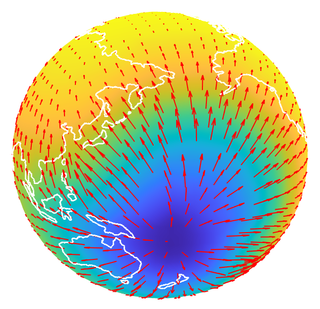
where $\beta_{1}=0.4$ , $\beta_{2}=0.3$ $\alpha_{1}=1.042$ , and $\alpha_{2}=2.089$ , and whose extended densities are then derived by using Equation (20). Figure 7 shows the source and target densities on $\mathbb{S}^{2}$ and the computed potential function with a quiver plot projected to $\mathbb{S}^{2}$ showing the direction of the gradient of the potential function overlaid on top of a world map outline. We chose the world map to allow the reader to more easily visualize the location of the mass density concentrations. It should be clear from formulation of the Optimal Transport problem in Equation (3) that in order to preserve mass the source mass located at the north pole needs to move to the target mass located at the south pole. In order to achieve this, the potential function must have a gradient near the north pole that points due south (towards the target mass distribution). Correspondingly, the direction of the mapping should point due south as well. This is precisely what we observe in Figure 7.

Analytical and computational problems arise for solving the Optimal Transport PDEs when the target mass density $g$ approaches zero in the computation domain. For one, the monotone discretizations on the sphere [22] requires that $g$ be bounded away from zero. For this computational example, we have $h=0.1$ and we can take the parameter $\beta_{1}$ smaller and smaller, for example, down to at least $\beta_{1}=0.01$ without much of an effect on the number of iterations to reach a given tolerance. However, from numerical experiments, we have found that the Algorithm works fine above $\beta_{2}=0.05=h/2$ , but not below this threshold, since the algorithm became unstable.

4.4.4. Peanut Reflector

In this example, we perform an Optimal Transport computation using the logarithmic cost $c(\mathbf{x},\mathbf{y})=-\log(1-\mathbf{x}\cdot\mathbf{y})$ arising in the reflector antenna problem, with $\epsilon=0.2$ and $h=0.1$ and $\sigma=1$ . In the reflector antenna problem, the computed potential function $u_{\epsilon}(\mathbf{z})$ is then used to construct the shape of a reflector $\rho$ via the expression:

(68)

\rho=P_{\mathbb{S}^{2}}(\mathbf{z})e^{-u_{\epsilon}(\mathbf{z})},\ \ \ \mathbf{z}\in T_{\epsilon}.

Note that the reflector is a sphere only when $u_{\epsilon}$ is constant. A constant potential function is the solution of the Optimal Transport problem on $\mathbb{S}^{2}$ only when $f=g$ . In the reflector antenna problem, light originating at the origin (center of the sphere) with a given directional light intensity pattern $f(\mathbf{x})$ impinges off a reflector with shape given in Equation (68), and then travels in a direction $\mathbf{m}(\mathbf{x})$ , yielding a far-field light intensity pattern $g(\mathbf{m}(\mathbf{x}))$ . Conservation of light intensity, the physical laws of reflection, and a change of variables allow one to solve for the reflector shape via the function $u$ in Equation (68) by solving for $u$ in the Optimal Transport PDE in Equations (8) and (9) with the logarithmic cost $c(\mathbf{x},\mathbf{y})=-\log(1-\mathbf{x}\cdot\mathbf{y})$ .

Strictly speaking, a reflector antenna should only be a hemisphere, since the intention is to redirect directional light intensity from the origin (inside the reflector) to the far-field outside the reflector. In order to do this, light must escape, and so the reflector cannot entirely envelop the origin. Temporarily putting physical realities aside, we compute the shape of the reflector for light intensity functions $f$ and $g$ with support equal to $\mathbb{S}^{2}$ , demonstrating that the computation can be done for the entire sphere for the cost function $c(\mathbf{x},\mathbf{y})=-\log(1-\mathbf{x}\cdot\mathbf{y})$ . We use a source density function which resembles a headlights of a car projected onto a sphere and a constant target density. The densities and the resulting “peanut-shaped” reflector is shown in Figure 8. This computation was inspired by the work in [46] and was also done with a different discretization in [23].

We perform another computation using the logarithmic cost function in order to compare with an exact solution. According to Appendix Appendix A: Axisymmetric Potential Functions on the unit sphere, if the source and target densities satisfy:

(69)		$\displaystyle f(x,y,z)$	$\displaystyle=\frac{\sin\left(\pi-\arccos(z)-\arccos\left(\frac{1-z^{2}-a_{0}^{2}}{1-z^{2}+a_{0}^{2}}\right)\right)}{4\pi\sqrt{1-z^{2}}}\left(-1+\frac{2a_{0}z}{1-z^{2}+a_{0}^{2}}\right),$
(70)		$\displaystyle g(x,y,z)$	$\displaystyle=\frac{1}{4\pi},$

then the potential function is known analytically to be:

(71)

u(x,y,z)=\frac{z}{a_{0}}.

We perform our computation using Algorithm 1, with $\epsilon=0.2$ , $h=0.05$ and $\sigma=8$ and the results are shown in Figure 9.

4.4.5. Non-Lipschitz target density

For this example, we have chosen $\epsilon=0.2$ and $h=0.1$ performed the computation on a grid of $5014$ points with $\sigma=1$ . We perform the computation for the squared geodesic cost function $c(\mathbf{x},\mathbf{y})=\frac{1}{2}d_{\mathbb{S}^{2}}(\mathbf{x},\mathbf{y})^{2}$ and for the following source and target density functions for Cartesian coordinates $(x,y,z)$ :

$\displaystyle f(x,y,z)$	$\displaystyle=(1-\beta_{1})\frac{1}{\alpha_{1}}e^{-5\arccos{x}^{2}}+\frac{\beta_{1}}{4\pi},$
$\displaystyle g(x,y,z)$	$\displaystyle=(1-\beta_{2})/2\pi,$	$\displaystyle\text{if}\ z\cdot\mathbf{n}\geq 0$
$\displaystyle g(x,y,z)$	$\displaystyle=\beta_{2}/4\pi,$	$\displaystyle\text{otherwise},$

where $\mathbf{n}=(0.2,0.2,1)$ , $\beta_{1}=0.3$ , $\beta_{2}=0.1$ and $\alpha_{1}=0.607788$ and the extended density functions are given by Equation (20). The target mass density in this example is discontinuous and the set of discontinuity has been chosen to not align with the computational grid $\mathcal{T}^{h}_{\epsilon}$ . This is an important and difficult test example since the target density, while bounded away from zero, is not Lipschitz. Figure 10 shows the source and target densities and the resulting quiver plot of the direction of the gradient of the potential function. Since we are performing a computation with the squared geodesic cost function, the gradient of the potential function around where the source mass is concentrated (middle of the Pacific Ocean) should be pointing to the northeast, but fanning out, so the mass gets appropriately spread out. This is, in fact, what we see from Figure 10.

4.4.6. Reflector antenna design using a hemisphere

As outlined in Section 3.6, we can use a modification of Algorithm 1 to solve Optimal Transport on the northern hemisphere of $\mathbb{S}^{2}$ , which is a surface with boundary, provided that we augment the discretization with zero-Neumann boundary conditions on the extension of the boundary. We use the density functions:

(72)		$\displaystyle f(x,y,z)$	$\displaystyle=\frac{1+10\arccos(z)}{2\pi(1+a_{0})},\ \ \$	$\displaystyle z\geq 0,$
(73)		$\displaystyle g(x,y,z)$	$\displaystyle=\frac{1}{2\pi},\ \ \$	$\displaystyle z\geq 0.$

For this computation, we use $\sigma=8$ , $\epsilon=0.2$ and $h=0.05$ . The resulting grid has $N=24208$ points. We perform this computation using the logarithmic cost function $c(x,y)=-\log(1-x\cdot y)$ , since this corresponds to a more physically accurate computation of the reflector antenna problem, as the computation is only for a light intensity pattern on one hemisphere. Even though, strictly speaking, a reflector antenna computation must be done over the entire sphere, we model a source light intensity pattern in the northern hemisphere being reflected to a target light intensity pattern in the southern hemisphere via a computation using the logarithmic cost function $c(x,y)=-\log(1-x\cdot y)$ only in the northern hemisphere.

The results of the computation are shown in Figure 11, which has a gradient of approximately zero along the boundary (strictly speaking the gradient is zero for the ghost points $\mathcal{C}^{h}$ which are located a distance $h$ below the boundary). The source mass, which is concentrated more around the equator, moves toward the north pole, as expected.

4.4.7. Optimal Transport computation on a torus

We consider the torus parametrized as follows:

(74)	$\displaystyle x$	$\displaystyle=\left(c+a\cos v\right)\cos u,$
(75)	$\displaystyle y$	$\displaystyle=\left(c+a\cos v\right)\sin u,$
(76)	$\displaystyle z$	$\displaystyle=a\sin u,$

for $u,v\in[0,2\pi)$ and $a=0.65$ and $c=1.3$ .

The signed distance function $\phi_{\Gamma}$ is given by the explicit formula:

(77)

\phi_{\Gamma}(\mathbf{z})=\sqrt{\left(\sqrt{x^{2}+y^{2}}-c\right)^{2}+z^{2}}-a,

and the projection operator $P_{\Gamma}$ is defined by the following map:

(78)

(x,y,z)\mapsto\left(\left(c+\frac{a}{\rho}(r-c)\right)\frac{x}{r},\left(c+\frac{a}{\rho}(r-c)\right)\frac{y}{r},\frac{a}{\rho}z\right).

We apply Algorithm 1, with $\epsilon=0.2$ , $h=0.05$ , and $\sigma=8$ , to solve the resulting discrete equations. The resulting grid has $N=106304$ points.

For cost functions that do not require pre-computation, the runtime of Algorithm 1 is similar for that on the sphere $\mathbb{S}^{2}$ . We will use the following cost function, since it does not require the expensive computation of geodesics on $\Gamma$ :

(79)

c_{\sigma}(\mathbf{z}_{1},\mathbf{z}_{2})=\frac{1}{2}\left\|P_{\Gamma}(\mathbf{z}_{1})-P_{\Gamma}(\mathbf{z}_{2})\right\|^{2}+\frac{\sigma}{2}\left(\phi_{\Gamma}(\mathbf{z}_{1})-\phi_{\Gamma}(\mathbf{z}_{2})\right)^{2}.

On a torus, given an appropriate potential function $u$ , the mapping for such a cost function satisfies:

(80)

\mathbf{m}(\mathbf{x})=\mathbf{x}+\nabla u(\mathbf{x})+\alpha\mathbf{n}(\mathbf{x}),

where $\alpha$ is the smallest value for which $\mathbf{m}(\mathbf{x})\in\Gamma$ . As this shows, the problem with such a cost function, though cheap, is that the source and target masses cannot require the mapping to transport mass too far, see [53] for more examples of cost functions that do not allow mass to be transported beyond a certain geodesic distance.

The source and target densities we use for this computation are:

(81)		$\displaystyle f(x,y,z)$	$\displaystyle=\frac{z+a+a_{0}}{4\pi^{2}ac(a+a_{0})},$
(82)		$\displaystyle g(x,y,z)$	$\displaystyle=\frac{1}{4\pi^{2}ac},$

for $(x,y,z)\in\Gamma$ , where $a_{0}=0.5$ . The source and target masses and computed potential function are shown in Figure 12.

The use of this cost function may be an efficient expedient for moving mesh methods on the torus, since any cost function used for Optimal Transport computations that yields a pushforward mapping is valid to use, see [54] for an overview of moving mesh methods using Optimal Transport. We implement a moving mesh computation on the torus for $a_{0}=1$ , where transported mesh is not necessarily symmetric to the grid due to the computational grid being generated differently than the mesh. The results are shown in Figure 13, which demonstrate that the density of mesh points on the top of the torus is decreasing, while the density of mesh points on the bottom of the torus is increasing. Also, the mesh does not exhibit tangling while keeping the same connectivity, another beneficial aspect of using Optimal Transport for moving mesh methods.

5. Conclusion

In this article, we have extended the Optimal Transport problem on a compact surface $\Gamma\subset\mathbb{R}^{3}$ onto a thin tubular neighborhood $T_{\epsilon}$ with width $\epsilon$ . We showed how one can then compute the Optimal Transport mapping $\mathbf{m}$ for the Optimal Transport problem on $\Gamma$ by solving instead for the Optimal Transport mapping $\bar{\mathbf{m}}$ which is the solution to the extended Optimal Transport problem on $T_{\epsilon}$ . The key is to extend the density functions and cost function in an appropriate way. The primary benefit of this extension is that the PDE formulation of the Optimal Transport problem on $T_{\epsilon}$ has only Euclidean derivatives. This allows us the flexibility to design a simple discretization that uses a Cartesian grid. We have discretized the extended PDE formulation of the Optimal Transport problem on $T_{\epsilon}$ and shown its ease of implementation and success with two different cost functions on the sphere, on the northern hemisphere of the sphere, where additional boundary conditions had to be implemented, and also on the $2$ -torus.

Acknowledgment

Tsai’s research is supported partially by National Science Foundation Grants DMS-2110895 and DMS-2208504.

Appendix A: Axisymmetric Potential Functions on the unit sphere

Axisymmetric potential functions $u$ of the Optimal Transport PDE on the sphere can be generated for both the squared geodesic $c(x,y)=\frac{1}{2}d_{\mathbb{S}^{2}}(x,y)^{2}$ and logarithmic cost $c(x,y)=-\log(1-x\cdot y)$ by specifying particular axisymmetric source $f$ and target $g$ density functions. For the squared geodesic cost, given that the potential function is axisymmetric, that is, if $u(\theta,\phi)=u(\theta)$ , then the Optimal Transport mapping satisfies $T(\theta,\phi)=\left(\theta^{\prime},\phi\right)$ . Using this, one can compute the determinant of the Jacobian of the Optimal Transport mapping $T$ for the squared geodesic cost as follows:

(83)

F(\theta):=\left|DT\right|=\left|\frac{\sin\theta^{\prime}}{\sin\theta}\right|\left|\frac{d\theta^{\prime}}{d\theta}\right|.

For the squared geodesic cost function $c(x,y)=\frac{1}{2}d_{\mathbb{S}^{2}}(x,y)^{2}$ , $\theta^{\prime}=\theta+\frac{du}{d\theta}$ , and $\theta^{\prime}\in[0,\pi]$ and therefore, we derive:

(84)

F(\theta)=\frac{\sin\left(\theta+\frac{du}{d\theta}\right)}{\sin\theta}\left|\frac{d}{d\theta}\left(\theta+\frac{du}{d\theta}\right)\right|=\frac{\sin\left(\theta+\frac{du}{d\theta}\right)}{\sin\theta}\left|1+\frac{d^{2}u}{d\theta^{2}}\right|.

In contrast to the derivation in [9], we are concerned not with the so-called “monitor function”, but instead with producing the density functions $f$ and $g$ that satisfy $f(\theta,\phi)=f(\theta)$ and $g(\theta,\phi)=g(\theta)$ . Furthermore, the measure-preserving property implies that $f$ and $g$ must satisfy the following Jacobian equation:

(85)

f(\theta)=F(\theta)g\left(\theta+\frac{du}{d\theta}\right).

To generate simple tests, let us take the target density to be constant, i.e. $g=1/4\pi$ , and we will solve for the source density function $f$ given a known smooth axisymmetric potential function $u$ . With a constant target density, the source density function $f$ must satisfy the following:

(86)

f(\theta)=\frac{F(\theta)}{4\pi}.

Now, given the axisymmetric potential function $u=\frac{\cos\theta}{a_{0}}$ , where $a_{0}>1$ , we get:

(87)

f\left(\theta\right)=\frac{\sin\left(\theta-\frac{\sin\theta}{a_{0}}\right)}{4\pi\sin\theta}\left(1-\frac{\cos\theta}{a_{0}}\right).

This integrates to $1$ over $\mathbb{S}^{2}$ , by Equation (85). Figure 14 shows what this density function looks like for $a_{0}=3$ .

The logarithmic cost is a little trickier. For example, “flat” potential functions (flat with respect to the standard metric on the sphere) lead to an Optimal Transport mapping $T$ which satisfies $T(\mathbf{x})=-\mathbf{x}$ . For an axisymmetric potential function, such a mapping will satisfy $T(\theta,\phi)=(\theta^{\prime},2\pi-\phi)$ . However, since our densities and potential function will be axisymmetric, we have $T(\theta,2\pi-\phi)=(\theta^{\prime},\phi)$ , so without loss of generality we may just compute $\theta^{\prime}$ for the Jacobian and not worry about what happens to the aximuthal coordinate $\phi$ . For the logarithmic cost, we get $\theta^{\prime}=\pi-\theta-\text{sgn}\left(\frac{du}{d\theta}\right)\arccos R\left(\frac{du}{d\theta}\right)$ , where $R(\xi)=\frac{\xi^{2}-1}{\xi^{2}+1}$ . In the axisymmetric case, we either have $\text{sgn}\left(\frac{du}{d\theta}\right)=\pm 1$ , since otherwise the mapping would map two or more points to the same point. The expression for the Jacobian is therefore:

(88)

F(\theta)=\frac{\sin\left(\pi-\theta+\text{sgn}\left(\frac{du}{d\theta}\right)\arccos R\left(\frac{du}{d\theta}\right)\right)}{\sin\theta}\left(-1+\text{sgn}\left(\frac{du}{d\theta}\right)\frac{d}{d\theta}\arccos R\left(\frac{du}{d\theta}\right)\right).

For the axisymmetric potential function $u=\cos\theta/a_{0}$ , so $\text{sgn}\left(\frac{du}{d\theta}\right)=-1$ , and thus, we compute:

(89)

R\left(\frac{du}{d\theta}\right)=\frac{\sin^{2}\theta-a_{0}}{\sin^{2}\theta+a_{0}},

and

(90)

f(\theta)=\frac{\sin\left(\pi-\theta-\arccos\left(\frac{\sin^{2}\theta-a_{0}^{2}}{\sin^{2}\theta+a_{0}^{2}}\right)\right)}{4\pi\sin\theta}\left(-1+\frac{2a_{0}\cos\theta}{\sin^{2}\theta+a_{0}^{2}}\right).

Figure 15 shows what this density function looks like for $a_{0}=3$ .

References

[1] E. Aamari, J. Kim, F. Chazal, B. Michel, A. Rinaldo, and L. Wasserman. Estimating the reach of a manifold. Electronic Journal of Statistics, 13(1):1359 – 1399, 2019.
[2] S. Ahmed, S. Bak, J. McLaughlin, and D. Renzi. A third order accurate fast marching method for the eikonal equation in two dimensions. SIAM Journal on Scientific Computing, 33(5):2402–2420, 2011.
[3] G. Bao and Y. Zhang. Optimal transportation for electrical impedance tomography. arXiv, 2022.
[4] G. Barles and P. E. Souganidis. Convergence of approximation schemes for fully nonlinear second order equations. Asymptotic Analysis, 4:271–283, 1991.
[5] M. Bauer, S. Joshi, and K. Modin. Diffeomorphic density matching by optimal information transport. Society for Industrial and Applied Mathematics Journal on Imaging Sciences, 8(3):1718–1751, 2015.
[6] J. Bedrossian, J. H. Von Brecht, S. Zhu, E. Sifakis, and J. M. Teran. A second order virtual node method for elliptic problems with interfaces and irregular domains. Journal of Computational Physics, 229(18):6405–6426, 2010.
[7] S. C. Brenner and M. Neilan. Finite element approximations of the three dimensional monge-ampère equation. ESAIM-Mathematical Modelling and Numerical Analysis, 46:979–1001, 2012.
[8] K. Brix, Y. Hafizogullari, and A. Platen. Designing illumination lenses and mirrors by the numerical solution of Monge-Ampère equations. Journal of the Optical Society of America A, 32(11):2227–2236, 2015.
[9] C. Budd, A. McRae, and C. Cotter. The scaling and skewness of optimally transported meshes on the sphere. Journal of Computational Physics, 375:540–564, December 2018.
[10] P. Castro, Q. Mérigot, and B. Thibert. Far-field reflector problem and intersection of paraboloids. Numerische Mathematik, 134(10), 2016.
[11] P. M. M. D. Castro, Q. Mérigot, and B. Thibert. Far-field reflector problem and intersection of paraboloids. Numerische Mathematik, 134:389–411, 2016.
[12] L. Cheng and R. Tsai. Redistancing by flow of time dependent eikonal equation. Journal of Computational Physics, 227, 2008.
[13] J. Chu and R. Tsai. Volumetric variational principles for a class of partial differential equations defined on surfaces and curves. Res Math Sci, 5(19), 2018.
[14] L. Cui, X. Qi, C. Wen, N. Lei, X. Li, M. Zhang, and X. Gu. Spherical optimal transportation. Computer-Aided Design, 115:181–193, 2019.
[15] M. Cuturi. Sinkhorn distances: Lightspeed computation of optimal transportation distances. Advances in Neural Information Processing Systems, 26, June 2013.
[16] L. L. Doskolovich, D. A. Bykov, A. A. Mingazov, and E. A. Bezus. Optimal mass transportation and linear assignment problems in the design of freeform refractive optical elements generating far-field irradiance distributions. Optics Express, 27(9):13083–13097, 2019.
[17] B. Engquist, A.-K. Tornberg, and R. Tsai. Discretization of dirac delta functions in level set methods. Journal of Computational Physics, 207(1):28–51, 2005.
[18] H. Federer. Curvature measures. Transactions of the American Mathematical Society, (93):418–491, 1959.
[19] T. Glimm and V. Oliker. Optical design of single reflector systems and the Monge-Kantorovich mass transfer problem. Journal of Mathematical Sciences, 117(3):4096–4108, 2003.
[20] B. D. Hamfeldt. Convergence framework for the second boundary value problem for the Monge-Ampère equation. Society for Industrial and Applied Mathematics Journal on Numerical Analysis, 57(2):945–971, January 2019.
[21] B. F. Hamfeldt and J. Lesniewski. Convergent finite difference methods for fully nonlinear elliptic equations in three dimensions. Journal of Scientific Computing, 90(35), March 2022.
[22] B. F. Hamfeldt and A. G. R. Turnquist. A convergent finite difference method for optimal transport on the sphere. Journal of Computational Physics, 445, November 2021.
[23] B. F. Hamfeldt and A. G. R. Turnquist. Convergent numerical method for the reflector antenna problem via optimal transport on the sphere. Journal of the Optical Society of America A, 38:1704–1713, 2021.
[24] B. F. Hamfeldt and A. G. R. Turnquist. A convergence framework for optimal transport on the sphere. Numerische Mathematik, 151:627–657, June 2022.
[25] J. L. Hellrung Jr, L. Wang, E. Sifakis, and J. M. Teran. A second order virtual node method for elliptic problems with interfaces and irregular domains in three dimensions. Journal of Computational Physics, 231(4):2015–2048, 2012.
[26] F. Izzo, O. Runborg, and R. Tsai. Convergence of a class of high order corrected trapezoidal rules. arXiv preprint arXiv:2208.08216, 2022.
[27] F. Izzo, O. Runborg, and R. Tsai. High-order corrected trapezoidal rules for a class of singular integrals. Advances in Computational Mathematics, 49(4):60, 2023.
[28] R. Kimmel, D. Shaked, N. Kiryati, and A. M. Bruckstein. Skeletonization via distance maps and level sets. Computer vision and image understanding, 62(3):382–391, 1995.
[29] C. Kublik and R. Tsai. Integration over curves and surfaces defined by the closest point mapping. Research in the mathematical sciences, 3(3), 2016.
[30] C. Kublik and R. Tsai. An extrapolative approach to integration over hypersurfaces in the level set framework. Mathematics of Computation, 2018.
[31] H. Lavenant, S. Claici, E. Chien, and J. Solomon. Dynamic optimal transport on discrete surfaces. ACM Transactions on Graphics (SIGGRAPH Asia 2018), 37(6), December 2018.
[32] J. Liang and H. Zhao. Solving partial differential equations on point clouds. SIAM Journal on Scientific Computing, 35(3), May 2013.
[33] G. Loeper. On the regularity of solutions of optimal transportation problems. Acta Mathematica, 202:241–283, 2009.
[34] X.-N. Ma, N. X. Trudinger, and X.-J. Wang. Regularity of potential functions of the optimal transportation problem. Archive for Rational Mechanics and Analysis, 177(2):151–183, 2005.
[35] C. B. Macdonald and S. J. Ruuth. The implicit closest point method for the numerical solution of partial differential equations on surfaces. SIAM Journal on Scientific Computing, 31(6):4330–4350, 2010.
[36] L. Martin and Y.-H. R. Tsai. Equivalent extensions of Hamilton–Jacobi–Bellman equations on hypersurfaces. Journal of Scientific Computing, 84(3):43, 2020.
[37] R. J. McCann. Polar factorization of maps on Riemannian manifolds. Geometric and Functional Analysis, 11:589–608, 2001.
[38] Q. Mérigot, J. Meyron, and B. Thibert. An algorithm for optimal transport beween a simplex soup and a point cloud. SIAM Journal on Imaging Sciences, 11(2):1363–1389, 2018.
[39] C. Min and F. Gibou. Geometric integration over irregular domains with application to level-set methods. Journal of Computational Physics, 226(2):1432–1443, 2007.
[40] C. Min and F. Gibou. A second order accurate level set method on non-graded adaptive cartesian grids. Journal of Computational Physics, 225(1):300–321, 2007.
[41] A. M. Oberman. Convergent difference schemes for degenerate elliptic and parabolic equations: Hamilton–Jacobi equations and free boundary problems. Society for Industrial and Applied Mathematics Journal on Numerical Analysis, 44(2):879–895, 2006.
[42] V. Oliker. Freeform optical systems with prescribed irradiance properties in near-field. In International Optical Design Conference 2006, volume 6342, page 634211, California, United States, 2006. International Society for Optics and Photonics.
[43] V. Oliker, J. Rubinstein, and G. Wolansky. Supporting quadric method in optical design of freeform lenses for illumination control of a collimated light. Advances in Applied Mathematics, 62:160–183, 2015.
[44] L. Romijn, J. ten Thije Boonkkamp, and W. IJzerman. Freeform lens design for a point source and far-field target. Journal of the Optical Society of America A, 36(11):1926–1939, 2019.
[45] L. B. Romijn. Generated Jacobian Equations in Freeform Optical Design: Mathematical Theory and Numerics. PhD thesis, Eindhoven University of Technology, 2021.
[46] L. B. Romijn, J. H. M. ten Thije Boonkkamp, and W. L. IJzerman. Inverse reflector design for a point source and far-field target. Journal of Computational Physics, 408:109283, 2020.
[47] S. Ruuth and B. Merriman. A simple embedding method for solving partial differential equations on surfaces. Journal of Computational Physics, 227(3):1943–1961, 2008.
[48] F. Santambrogio. Optimal Transport for Applied Mathematicians, volume 55. Birkhäuser, Basel, Switzerland, 2015.
[49] H. Schaeffer and T. Y. Hou. An accelerated method for nonlinear elliptic PDE. Journal of Scientific Computing, 69(2):556–580, 2016.
[50] J. A. Sethian. Fast marching methods. SIAM Review, 41(2):199–235, 1999.
[51] J. Solomon, R. Rustamov, L. Guibas, and A. Butscher. Earth mover’s distances on discrete surfaces. Association for Computing Machinery Transactions on Graphics, 33(4):1–12, July 2014.
[52] Y.-H. R. Tsai. Rapid and accurate computation of the distance function using grids. Journal of Computational Physics, 178(1):175–195, 2002.
[53] A. G. R. Turnquist. Optimal transport with defective cost functions with applications to the lens refractor problem. arXiv preprint arXiv:2308.08701, August 2023.
[54] A. G. R. Turnquist. Adaptive mesh methods on compact manifolds via optimal transport and optimal information transport. Journal of Computational Physics, 500(112726), March 2024.
[55] J. Urbas. On the second boundary value problem for equations of Monge-Ampère type. Journal für die reine und angewandte Mathematik, 487:115–124, 1997.
[56] X.-J. Wang. On the design of a reflector antenna. IOP Science, 12:351–375, 1996.
[57] X.-J. Wang. On the design of a reflector antenna II. Calculus of Variations and Partial Differential Equations, 20(3):329–341, 2004.
[58] H. Weller, P. Browne, C. Budd, and M. Cullen. Mesh adaptation on the sphere using optimal transport and the numerical solution of a Monge-Ampère type equation. Journal of Computational Physics, 308:102–123, 2016.
[59] R. Wu, L. Xu, P. Liu, Y. Zhang, Z. Zheng, H. Li, and X. Liu. Freeform illumination design: a nonlinear boundary problem for the elliptic Monge-Ampére equation. Optics Letters, 38(2):229–231, 2013.
[60] N. K. Yadav. Monge-Ampère Problems with Non-Quadratic Cost Function: Application to Freeform Optics. PhD thesis, Technische Universiteit Eindhoven, Eindhoven, Netherlands, 2018.
[61] J. Yu, R. Lai, W. Li, and S. Osher. Computational mean-field games on manifolds. Journal of Computational Physics, 484(112070), July 2023.
[62] Y.-T. Zhang, H.-K. Zhao, and J. Qian. High order fast sweeping methods for static Hamilton-Jacobi equations. Journal of Scientific Computing, 29(1):25–56, 2006.
[63] Y. Zhong, K. Ren, O. Runborg, and R. Tsai. Error analysis for the implicit boundary integral method. arXiv preprint arXiv:2312.07722, 2023.

A Volumetric Approach to Monge’s Optimal Transport on Surfaces

Abstract.

1. Introduction

2. Background

Definition 1.

Definition 2.

Theorem 3.

Remark.

3. Volumetric Extension of the Optimal Transport Problem

3.1. The general setup

3.2. Extension of Surface Densities

3.3. Extension of Cost Function to TϵT_{\epsilon}

3.4. Equivalence of the Two Optimal Transport Problems

Theorem 4.

Corollary 5.

Proof.

Mass preservation

cσc_{\sigma}-Convexity of the Potential Function

Lemma 6.

Proof.

3.5. Example: Optimal Transport on the Unit Sphere

Case 1: c​(𝐱,𝐲)=12​d𝕊2​(𝐱,𝐲)c(\mathbf{x},\mathbf{y})=\frac{1}{2}d_{\mathbb{S}^{2}}(\mathbf{x},\mathbf{y}) is the the squared geodesic distance between 𝐱\mathbf{x} and 𝐲\mathbf{y} on the unit sphere.

Case 2: c​(𝐱,𝐲)=−log⁡(1−𝐱⋅𝐲)c(\mathbf{x},\mathbf{y})=-\log(1-\mathbf{x}\cdot\mathbf{y}), the logarithmic cost function appearing in the reflector antenna problem.

3.6. Optimal Transport on Surfaces with Boundary

4. Computational Examples

4.1. Geometry processing

4.2. Discretization of the PDEs

Definition 7.

Remark.

Remark.

4.3. Computational Complexity

4.4. Computational Results

4.4.1. Comparison with the analytical solution on the sphere

4.4.2. Studies with Varying σ\sigma, ϵ\epsilon, and hh

4.4.3. Optimal transport on a sphere: from North Pole to South Pole

4.4.4. Peanut Reflector

4.4.5. Non-Lipschitz target density

4.4.6. Reflector antenna design using a hemisphere

4.4.7. Optimal Transport computation on a torus

5. Conclusion

Acknowledgment

Appendix A: Axisymmetric Potential Functions on the unit sphere

References

3.3. Extension of Cost Function to $T_{\epsilon}$

$c_{\sigma}$ -Convexity of the Potential Function

Case 1: $c(\mathbf{x},\mathbf{y})=\frac{1}{2}d_{\mathbb{S}^{2}}(\mathbf{x},\mathbf{y})$ is the the squared geodesic distance between $\mathbf{x}$ and $\mathbf{y}$ on the unit sphere.

Case 2: $c(\mathbf{x},\mathbf{y})=-\log(1-\mathbf{x}\cdot\mathbf{y})$ , the logarithmic cost function appearing in the reflector antenna problem.

4.4.2. Studies with Varying $\sigma$ , $\epsilon$ , and $h$