A virtual element method for the elasticity problem allowing small edges
Abstract.
In this paper we analyze a virtual element method for the two dimensional elasticity problem allowing small edges. With this approach, the classic assumptions on the geometrical features of the polygonal meshes can be relaxed. In particular, we consider only star-shaped polygons for the meshes. Suitable error estimates are presented, where a rigorous analysis on the influence of the Lamé constants in each estimate is presented. We report numerical tests to assess the performance of the method.
Key words and phrases:
Elasticity equations, eigenvalue problems, error estimates2000 Mathematics Subject Classification:
Primary 35J25, 65N15, 65N30, 65N12,74B05, 76M101. Introduction
The virtual element method (VEM) is a numerical approach that has taken relevance in the community of numerical analysis in the nowadays, since t allows to approximate the solutions of partial differential equations with accuracy together with a computational implementation that results to be easy to handle. Moreover, the flexibility of this method on the geometrical assumptions on the elements of the meshes, which permits arbitrary polygonal elements such as convex and nonconvex polygons, and hanging nodes, that are not allowed in the finite element approach, just for mention the most relevant. These considerations, lead the VEM to be a suitable alternative to approximate physical phenomenons that the standard finite element method is not possible to consider, such as domains with fractures, cuspids, holes, etc. A full treatment of the basic elements of the VEM is available in [6, 7].
In recent years, different studies have been carried out that demonstrate the good performance of VEM on problems of different natute, such as evolutionary problems, spectral problems, nonlinear problems, among others. For a better knowledge of the recent state of art we resort to [2]. Now, in the continuous advance in the research of virtual methods, a new approach has been developed that allows the use of even more general and flexible meshes. This new approach for the VEM is now related to consider small edges for the polygonal elements on the meshes, as is presented in [8, 10, 12]. More precisely, depending on the regularity of the solution of the partial differential equations, is possible to only consider star shaped polygonal elements, or a bounded number of edges for the polygons. In both cases these assumptions are enough to allow sufficiently small sides on the elements. To make matter precise, in [8] the authors have developed this new strategy considering the Laplace operator in two dimensions, whereas in [10] have been capable to extend the ideas for three dimensions, proving that VEM with small edges also works when more complicated domains are considered.
The aim now is to analyze the performance of the VEM with small edges in other contexts, in fact, this research is in ongoing progress. For instance, in [17] an application of this new approach in eigenvalue problems has shown the accuracy of the approximation of the spectrum for the Steklov eigenvalue problem, in [24] for elliptic interface problems, [14] for three dimensional problems considering polytopal meshes, etc.
In the present paper, our contribution is to apply the methodology of small edges for the two dimensional linear elasticity problem. The bibliography related to numerical methods to approximate the displacement of some elastic structure is abundant, where different method as been proposed, as [5, 11, 13, 15, 18, 19, 25], where mixed finite element methods, mixed virtual element methods, stabilized methods, discontinuous Galerkin methods, just for mention some of them, have been considered. Regarding the study of VEM applied to elasticity problems, we can cite the following works [3, 4, 20, 22, 23, 26, 27]. In particular, a VEM for the primal formulation of the elasticity eigenvalue problem as been proposed in [20], where the proposed virtual spaces on this reference are a suitable alternative for the load problem. These virtual spaces for the elasticity equations, together with the small edges approach, are the core of our contribution.
In our paper, we are interested in the primal formulation of the linear elasticity equations with vanishing Dirichlet boundary condition. This boundary condition is needed for our purposes, since lead to the precise regularity that the small edges approach needs to be performed.
It is well known that the primal formulation for linear elasticity leads to the so called locking phenomenon when finite element families to discretize are implemented, which not occurs when mixed formulations are considered. This locking is due to the effects of the Poisson ratio, which we denote by , on the computation of the Lamé coefficient : if tends to , then goes to infinity. Then, it is important to have a correct control and knowledge on the constants that appear on the estimates when the mathematical analysis is performed. Moreover, the numerical tests that we will present lead to the conclusion that, regardless of the family of polygonal mesh under consideration, the convergence errors are not deteriorated; however, when tends to , the deterioration of the error curves is observed.
With this consideration, for the small edges approach we need to take care on this Lamé coefficient as with any other family of elements that discretizes . Moreover, the small edges approach that we will consider to run the analysis is based in the results of [10]. Hence, we need to adapt the theory, already available for the Laplace operator, for the elasticity operator. This obligates to have a spacial treatment on this context due the Lamé constants, specially .
The outline of this manuscript is as follows. In Section 2 the model problem that we consider in our paper, summarizing the results that are needed along our studies, together with definitions and notations to develop the mathematical analysis. The core of our manuscript is contained in Section 3, where we introduce the virtual element method of our interest. Under the assumption that the meshes allow small edges for the elements, we prove a series of technical results that are needed for the elasticity operator. These results contain important information related to how the physical parameters, inherent on the linear elasticity equations, are involved on the estimates associated to projections, interpolant operators and error estimates, among others. Finally, in Section 4, we report numerical tests, that illustrate the theory and exhibit the performance of the proposed method.
2. The model problem
Let be a convex, bounded, and open Lipschitz domain with boundary . The linear elasticity problem is as follows
| (2.1) |
where u represents the displacement of the solid, f is an external load, represents the density of the material that we assume constant, represents the strain tensor, and is the Cauchy tensor. The strain and Cauchy tensors are related through the operator , where and, which according to Hooke’s law, is defined by
where is the identity matrix, and and are the Lamé coefficients defined by
where is the Young’s modulus and is the Poisson ratio. Let us remark that when , then , which is an important issue that we need to take in consideration for our purposes. The variational formulation of (2.1) is the following: Given , find such that
| (2.2) |
Let us define the symmetric and continuous bilinear form
| (2.3) |
and the linear functional
| (2.4) |
Note that , and , proving that and are bounded. Now, with (2.3) and (2.4) at hand, we rewrite (2.2) as follows
Problem 1.
Given , find such that
From Korn’s inequality and Lax-Milgram’s lemma we have that Problem 1 is well posed and its solution satisfies , where is independent of . Moreover, from [16], the following regularity holds.
Lemma 2.1.
For every , the solution of Problem 1 is such that . Moreover, there exists such that .
3. The virtual element method
In the present section we introduce the virtual element method that we consider to approximate the solution of Problem 1. To do this task, we will consider a more relaxed conditions compared with those introduced in [6] for the classic VEM, where there is no possible to assume more general polygonal meshes allowing arbitrary edges, more precisely, small edges. Hence, and inspired in [8], if represents a family of polygonal meshes to discretize , is an arbitrary element of the mesh, and represents the mesh size. On the other hand, let . If and with , we define the relation . Then, from now and on, we will assume that for , there holds that and .
Let us assume the following assumption on :
-
A1.
There exists such that each polygon is star-shaped with respect to a ball with center and radius .
We denote by the number of vertices of .
Let us write the bilinear form and the functional as follows
where ,
where .
3.1. Virtual spaces
Now we introduce the virtual spaces of our interest. Following [1] and [8], we introduce the following local spaces
,
.
For each, , we introduce the projection defined for every as the solution of (see [27] for instance)
Definition 1.
We define the local virtual space by
,
where the space denotes the polynomials in in which are orthogonal to with respect to the product. We choose the same degrees of freedom as those in [6, Section 4.1] for the local virtual space defined above.
Now we are in position to introduce the global virtual space which we define by
For the analysis of the VEM allowing small edges, we introduce the following seminorm which is induced by the stability term defined by (see [10, equation (3.9)])
| (3.5) |
where represents the set of edges of , is the orthogonal projection onto the space and is the orthogonal projection onto the space . This seminorm will appear naturally when we operate to control the approximation errors of the virtual solutions, in particular to bound the norms of the polynomial projectors and the interpolations of the solutions. From the following trace inequality
| (3.6) |
and (3.5), there holds that
On the other hand, from Korn’s inequality and the fact that is bounded, we have
| (3.7) |
The following result is an adaptation of [10, Lemma 3.4] to our case, and gives an estimate for in terms of .
Lemma 3.1.
There holds
where the hidden constant is independent of .
Proof.
Let . Then, using the definition of , integration by parts, the definitions of and , inverse estimates and trace inequalities, we have
From the definition of we have
and invoking the estimate we obtain directly the following estimate for the seminorm of the projection
| (3.8) |
On the other hand, notice that from the definition of , the definition of and the fact that , we have
| (3.9) |
where in the first inequality, we have used Cauchy-Schwarz inequality and the fact that . Hence, from the following Poincaré-Friedrich inequality
| (3.10) |
and using (3.8) and (3.9), we obtain
This concludes the proof. ∎
Now we need approximation properties for . In the following result we derive such an estimates, that are an adaptation of those in [10, Lemma 3.5], in which we emphasize that the estimates depends on the Lamé coefficients.
Lemma 3.2.
The following estimates hold
-
i)
For all and , there holds
-
ii)
For all and , there holds
-
iii)
For all and , there holds
where in each estimate, the hidden constants are independent of .
Proof.
Let us recall the following Bramble-Hilbert estimate
| (3.11) |
We begin by proving ii). To do this task, given arbitrary, and invoking estimate (3.7) we have
From triangle inequality and (3.11), we have
Now to derive i), invoking (3.10), ii) and the definition of , for each we have
Finally, from the following polynomial approximation property (see [9, (4.5.3) Lemma])
| (3.12) |
together with (3.7), yields to
Then, given arbitrary, triangle inequality and (3.11), we obtain
concluding iii) and hence, the proof. ∎
In the previous result, we have made clear the dependence of the Lamé constants on the estimates. This is important to take into account, since in particular leads to numerical locking. Now, we are going to analyze stability and approximation properties for the orthogonal projector onto the space .
Remark 3.1.
The following estimate for holds
| (3.13) |
Moreover, since for all , as a consequence of (3.11) there holds
| (3.14) |
The following lemma is adapted from [10, Lemma 3.6] to our case, and states an estimate for the seminorm of .
Lemma 3.3.
There holds
where the hidden constant is independent of .
Proof.
The following result is adapted from [10, Lemma 3.7], and gives us an approximation for in seminorm .
Lemma 3.4.
The following estimate holds
where the hidden constant is independent of .
Proof.
Now we prove a stability result for norm of the projection with respect to the triple norm , for virtual functions. A similar result can be found in [10, Lemma 3.8] for the Laplace problem.
Lemma 3.5.
There holds
where the hidden constant is independent of .
Proof.
To prove the following result, we need to adapt the arguments of the proof of [10, Lemma 3.9] for the vectorial case, taking into account that now, in the estimates, the Lamé constants appear naturally.
Lemma 3.6.
Assume that A1 holds. Then, there exists a constant depending on and such that
Proof.
The proof is similar to what was done in [10, Lemma 3.9], since the two-dimensional case is direct. Then, we have
where , the operator , called lifting operator, was introduced in [10, Section 2.7], and was defined in the proof of [10, Lemma 3.9]. Therefore, from triangle inequality and Lemma 3.5 we have
| (3.15) |
Hence, we conclude that
| (3.16) |
where was defined in the proof of [10, Lemma 3.9], and (3.16) is obtained from [10, Lemma 3.9], together with (3.15). ∎
As a direct consequence of lemma above, we have the following result.
Corollary 3.1.
Assume that A1 holds. Then, there exists depending on y , such that
where denotes the tangential derivative of .
Proof.
3.2. The interpolation operator
In order to obtain error estimates for our numerical method, and interpolation operator is needed. This operator is defined locally, and its construction is based in the references [21] and [8], where this last reference makes the construction of this operator for the small edges approach.
We consider for the interpolation operator , which satisfies that the degrees of freedom of and are the same, together with the identity and
The following result is a stability estimate for in norm and its proof is straightforward from [10, Lemma 3.12].
Lemma 3.7.
Assume that A1 holds. Then, there holds
where the hidden constant depends on and , but not on .
We have the following estimate for . This result is adapted from [10, Lemma 3.13] to our case.
Lemma 3.8.
The following estimate hold
where the hidden constant depends on and .
Proof.
We also have a stability result for in norm, which is adapted from [10, Lemma 3.14].
Lemma 3.9.
The following estimate hold
where the hidden constant depends on and .
Proof.
Let . From triangle inequality we obtain
| (3.17) |
Now the aim is to estimate each term on the right hand side of (3.17). Invoking item i) of Lemma 3.2 with and Lemma 3.8, we have
| (3.18) |
On the other hand, from Lemmas 3.1 and 3.7 we have
| (3.19) |
Finally, replacing (3.18) and (3.19) in (3.17), we conclude the proof. ∎
The following result establishes approximation properties for . This results are adapted from those in [10, Lemma 3.15], and we again emphasize that the Lamé coefficients appears in our estimates.
Lemma 3.10.
For and , the following estimates hold
-
i)
,
-
ii)
,
-
iii)
,
where the hidden constants depend on and .
Proof.
First we prove i). We observe that, from Lemmas 3.1, 3.7 and 3.8, we have the estimate
Therefore, applying triangular inequality and invoking (3.11), we conclude that
To prove ii), we invoke (3.7) and Lemma 3.8, in order to obtain
Hence, applying triangular inequality and invoking (3.11), we obtain
Finally, for iii), we use (3.12), (3.7) and Lemma 3.8 to obtain
Therefore, applying triangular inequality and (3.11), we have
This concludes the proof.
∎
The following result is adapted from [10, Lemma 3.16] to our case, and gives us an approximation property for the interpolant operator , when . We will need this results to demonstrate properties about the operator and its discrete counterpart.
Lemma 3.11.
The following estimate holds
where the hidden constant depends on and .
Proof.
The following result is straightforward from [10, Lemma 3.18] which is essential to prove that the discrete bilinear form is elliptic in .
Lemma 3.12.
The following estimate holds
where the hidden constant is independent of
The following result establishes an estimate for , with , and its proof is naturally extended to our vectorial case, from the proof of [10, Lemma 3.19].
Lemma 3.13.
For every that vanishes in some part of , there holds
where the hidden constant depends only on .
Remark 3.2.
Let us introduce the following stabilization term defined for by
which corresponds to a scaled inner product between and in . Let us introduce the discrete bilinear form defined by
Now we define the following discrete operator
| (3.21) |
where is defined by
where is the piecewise discontinuous polynomial space of degree respect to and is the global -projector, such that . Finally, is the global projector with respect to , such that .
Now, we can write the virtual element discretization of Problem 1.
Problem 2.
Given , find such that
Remark 3.3.
Observe that from triangle inequality and (3.20), there holds
Moreover, the following estimate holds
| (3.22) |
It is easy to check that is elliptic in and hence, we deduce that Problem 2 has unique solution as a consequence of Lax-Milgram’s Lemma.
Now for the functional defined in (2.4) and its discrete counterpart defined in (3.21), we have the following approximation result (see [10, Lemma 4.1]).
Lemma 3.14.
Let . The following estimates hold true
-
i)
For all and for all ,
-
ii)
For all and for all ,
where the hidden constants are independent of .
Proof.
To conclude this section, we introduce the broken -seminorm with respect to , given by
3.3. Error estimates
Now our aim is to obtain error estimates for the proposed method. Clearly, due the previous results, the error estimates will depend on the Lamé coefficients. This fact gives us the hint that the error estimates that we can derive will not be optimal when the Poisson ratio is close to .
We introduce the energy norm defined by , and let us recall the following standard estimate (see [9] for instance)
| (3.23) |
The main task now is to estimate correctly the supremum in (3.23). With this aim in mind, we begin with the following result that states an approximation for the elliptic projector in the energy norm.
Remark 3.4.
For any , from the definition of and , the following estimate holds
| (3.24) |
Let us recall estimate (3.23). Now our task is to estimate each of the terms on its right hand side. With this goal in mind, let us begin by recalling that from the definition of and for each we have
Therefore, applying the Cauchy Schwarz inequality, (3.24) and the continuity of , we obtain
where . Hence, we have
with . On the other hand, there holds
and therefore we obtain
| (3.25) |
Now, using the results of the previous sections, we can give an error estimate in norm, under the assumption that u belongs to , with . From i) of Lemma 3.14 and 2.1, we have
| (3.26) |
On the other hand, from of Lemma 3.2, there holds
in which we derive
| (3.27) |
Now, to estimate , we put and . Then, we have
First, from item of Lemma 3.10 and (3.7), we obtain
On the other hand, using the estimate
applied to the -order derivatives of u, and standard interpolation estimates, we obtain
Finally, applying the polynomial estimate together with (3.7) and ii) of Lemma 3.10, we obtain
Then, there holds
| (3.28) |
with .
As a final task, we provide an estimate for . From the definition of and , (3.6) and Lemma 3.2, we have
Hence, we derive the estimate
| (3.29) |
The above estimates give us the following result, that is an adaptation of [10, Theorem 4.1], and we emphasize that the Lamé coefficients appears.
Theorem 3.1.
Assuming that the solution u of Problem 1 belongs to for . Then, the following estimate holds
where the constants is given by
and the hidden constant is independent of .
We also have the following result, that give us an error estimate for and in seminorm. This result is adapted from [10, Theorem 4.2] to our case.
Theorem 3.2.
Assuming that the solution u of Problem 1 belongs to , . Then, there holds
where is a positive constant depending on the Lamé coefficients.
Proof.
Note that, from the definition of and Theorem 3.1, we have
This gives us the following estimate
Therefore, applying triangular inequality and (3.27), we obtain
| (3.30) |
where . On the other hand, applying triangular inequality, Lemma 3.3 and (3.27), we deduce that
| (3.31) |
Finally, from triangular inequality, (3.22), (3.28), Theorem 3.1, and ii) of Lemma 3.10, we obtain
| (3.32) |
with
Therefore, we conclude the proof from (3.30), (3.31) y (3.32). ∎
Now, we will prove two results involving the stability term . These results are adapted respectively from [10, Lemma 4.2] and [10, Lemma 4.3], to our case.
Lemma 3.15.
For all , there holds
Lemma 3.16.
Assume that , . Then there holds
where is a positive constant depending on the Lamé coefficients.
Proof.
The following lemma is adapted from [10, Lemma 4.4], and gives us a consistency result.
Lemma 3.17.
Assuming that with . Then, there holds
where is a positive constant depending on the Lamé coefficients.
Proof.
From the linearity of , the definition of , Problems 1 and 2, we have
| (3.34) |
Now, from item ii) of Lemma 3.14 we have
| (3.35) |
On the other hand, applying Cauchy Schwarz inequality, and Lemmas 3.15 and 3.16, we obtain
| (3.36) |
with . Finally, invoking the Cauchy Schwarz inequality, Theorems 3.1 and 3.2, and part ii) of Lemma 3.10 yields to
| (3.37) |
where . Thus, from (3.34), (3.35), (3.36) and (3.37) allows us to conclude
with . This concludes the proof. ∎
The following result is an adaptation of [10, Theorem 4.3] to our case, and gives us an error estimate in norm.
Theorem 3.3.
Assuming that , , there holds
where the hidden constant depends on and not on , and is a positive constant depending on the Lamé coefficients.
Proof.
Let the solution of
Then, we have
Since we are assuming that is convex, and invoking Lemma 2.1, we have the following estimate for the seminorm
| (3.38) |
Then, from the continuity of , part ii) of Lemma 3.10, and Theorem 3.2 we obtain
where . Therefore, from (3.38) and Lemma 3.17 we obtain
where . This concludes the proof. ∎
Finally, we conclude this section with the following result, that gives us an error estimate for and in norm. This result is adapted from [10, Theorem 4.4] to our case.
Theorem 3.4.
Assuming that , , there holds
where is a positive constant depending on the Lamé coefficients.
Proof.
First, using triangular inequality, (3.14) and Theorem 3.3, we obtain
| (3.39) |
On the other hand, applying triangular inequality again, we have
Hence, from Lemma 3.1, (3.5) and (3.6), we deduce that
Therefore, we obtain the estimate
| (3.40) |
Now, from Lemma 3.10 we obtain
| (3.41) |
and by Theorems 3.2 and 3.3, there holds
| (3.42) |
with . Hence, from (3.40), (3.41) and (3.42) we conclude that
| (3.43) |
where . Finally, from i) of Lemma 3.10, we derive
| (3.44) |
Therefore, from (3.43) and (3.44) we obtain
| (3.45) |
with . Hence, we conclude from (3.39) and (3.45) that
where . This concludes the proof. ∎
4. Numerical experiments
In the following section we report a series of numerical experiments in which we illustrate the performance of the proposed numerical method. The results have been obtained with a MATLAB code.
To make matters precise, we are interested in the computation of experimental rates of convergence for the load problem, where we measure the error of approximation in the and norms. Moreover, as we have claimed through our study, the Poisson ratio is not allowed to be equal to , since the Lamé coefficient tends to infinity. Then, we will focus on values of far enough from , in order to obtain the desire results, and avoid the locking phenomenon. Let us remark that in all our numerical tests, we have taken as material density and Young modulus .
4.1. The unit square
We begin with a simple convex domain as the unit square . The boundary condition for the forthcoming tests is on the whole boundary . This configuration for the domain leads to solutions that are smooth enough on , except for values of , too close to .
The polygonal meshes that we will consider for our tests are the following:
-
: Triangles with small edges.
-
: Deformed triangles with middle points.
-
: Deformed squares.
-
: Voronoi,
and in Figure 1 we present examples of these meshes.


Les us mention that has the particularity that, for some element , the vertices are admissible to be very close between them, in order to almost collapse. This characteristic that can be observed in Figure 2 is the flexibility that the meshes with small edges allows, making a significant improvement from the classically admissible meshes. In Figure 2, we present the way in which the elements on are constructed: From a triangular mesh, we consider the middle point of each edge of the element as a new degree of freedom. Then, we move such a point on each edge to a distance from one vertex of and from the other where is the length of the edge , resulting a 6 edges polygon.

.
We remark that each of these meshes have the condition of our interest: the polygons are allowed to consider small edges as is claimed in assumption A1.
We begin by comparing the performance of the proposed method with two different stabilizations , in order to observe if there are significant differences when the small edges method is considered.
4.2. The derivative stabilization
The following results have been obtained with the following stabilization term
| (4.46) |
This stabilization is the one considered in, for instance, [8] for the Laplace source problem and [17] for the Steklov eigenvalue problem. With this stabilization, we perform the computation of the convergence orders for the elasticity problem for different values of the Poisson ratio and hence, different values of the Lamé coefficient . We remark that each load term is different for each value of .
In Figures 3 and 4 we report error curves for our method, where the meshes presented in Figure 1 have been considered. In these figures, the Poisson ratio takes the values and we observe that the error of the displacement in the norm and the seminorm decay when the mesh is refined. Moreover, this decay of the error occurs with the optimal order, as is expected according to our theory. However, we observe that when and are considered, the error estimate is not completely optimal. This is expectable since as we have claimed along our paper, when is close to the method is unstable. Moreover, is not an uniform mesh compared with the rest of the considered meshes, leading to geometrical issues that also may affect the convergence order for a Poisson ratio close to .
These results allow us to infer that the small edges approach, together with the stabilization term (4.46), perform an accurate approximation of the solution, independently of the polygonal mesh under consideration.


4.3. The classic stabilization
Now our aim is to compare the results obtained with the stabilization defined in (4.46), with the classic stabilization that us used in the VEM. To make matters precise, the stabilization term for the following tests is given by
| (4.47) |
which corresponds to the evaluation on the vertices of the polygons.
In what follows, we report error curves for the norm and seminorm when the stabilization (4.47) is considered. These results have obtained, once again, for and the meshes presented in Figure 1.


From Figures 5 and 6 we observe that the error in norm and seminorm behave according to the theory, when the different Poisson ratios are involved in the computation of the solution. This allows us to conclude that our small edges approach for the elasticity equations, works well independent of the stabilization implemented on the computation al codes, reinforcing the idea that the VEM, and particularly the small edges approach, is a versatile tool that approximates accurately the solutions of the elasticity equations.
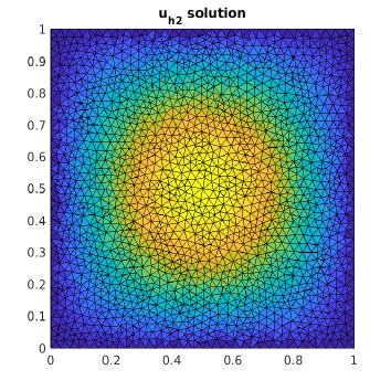
Finally in Figures 7 and 8 we present plots of the magnitude of the displacement, where components of the approximated and exact solutions are presented.


In order to confirm the robustness of the method, we present an additional experiment where we consider a mesh that we denote by , which consists in the union of three different Voronoi mesh. This mesh has the particularity that, where the meshes are glued, the nodes are sufficiently close each other, appearing polygons with arbitrary small edges. In Figure 9 we present an example of this mesh.

In Figure 10, we present the plots of computed error for mesh and different values of Poisson ratio, namely . Also, we present this experiment considering both stabilization terms (4.46) and (4.47).


The results clearly show that the method is strongly precise with this more general mesh and for the Poisson ratios. More precisely, there are no significant differences for these meshes when we compare the results with the ones obtained when , , , and are considered. Moreover, the stabilizations (4.46) and (4.47) work similarly.
4.4. Nonconvex domain
Now we perform a test that goes beyond the theory that we have developed, which assumes the convexity of the domain in order to obtain optimal order of convergence for the proposed VEM method. For this test, we consider a nonconvex domain that we call the L-shaped domain as is defined by . Clearly the geometry of this domain presents a geometrical singularity that leads to approximate a solution for the elasticity problem that is no sufficiently smooth. Hence, the VEM method will be not capable to achieve the optimal order of convergence under this configuration.
The polygonal meshes that we will consider for our tests are the following:
-
: Triangles with small edges.
-
: Deformed triangles with middle points.
-
: Voronoi-squares-deformed squares mixed.
-
: Voronoi.
In Figure 11 we present examples of these meshes when the L-shaped domain is considered.


For our experiments, we will consider the classic stabilization term (4.47). In what follows, we report error curves for the norm and seminorm when the stabilization (4.47) is considered. These results have obtained for and the meshes presented in Figure 11.


Finally in Figure 14 and Figure 15 we present plots of the magnitude of the displacement, where components of the approximated and exact solutions are presented.


References
- [1] B. Ahmad, A. Alsaedi, F. Brezzi, L. Marini, and A. Russo, Equivalent projectors for virtual element methods, Comput. Math. Appl., 66 (2013), pp. 376–391.
- [2] P. Antonietti, L. Beirão da Veiga, and G. Manzini, The Virtual Element Method and its Applications, vol. 31, SEMA SIMAI Springer Series, 2022.
- [3] E. Artioli, L. Beirão da Veiga, C. Lovadina, and E. Sacco, Arbitrary order 2D virtual elements for polygonal meshes: part I, elastic problem, Comput. Mech., 60 (2017), pp. 355–377.
- [4] E. Artioli, S. de Miranda, C. Lovadina, and L. Patruno, A dual hybrid virtual element method for plane elasticity problems, ESAIM Math. Model. Numer. Anal., 54 (2020), pp. 1725–1750.
- [5] T. P. Barrios, G. N. Gatica, M. González, and N. Heuer, A residual based a posteriori error estimator for an augmented mixed finite element method in linear elasticity, M2AN Math. Model. Numer. Anal., 40 (2006), pp. 843–869 (2007).
- [6] L. Beirão da Veiga, F. Brezzi, A. Cangiani, G. Manzini, L. D. Marini, and A. Russo, Basic principles of virtual element methods, Math. Models Methods Appl. Sci., 23 (2013), pp. 199–214.
- [7] L. Beirão da Veiga, F. Brezzi, L. D. Marini, and A. Russo, The hitchhiker’s guide to the virtual element method, Math. Models Methods Appl. Sci., 24 (2014), pp. 1541–1573.
- [8] L. Beirão da Veiga, C. Lovadina, and A. Russo, Stability analysis for the virtual element method, Math. Models Methods Appl. Sci., 27 (2017), pp. 2557–2594.
- [9] S. C. Brenner and L. R. Scott, The mathematical theory of finite element methods, vol. 15 of Texts in Applied Mathematics, Springer, New York, third ed., 2008.
- [10] S. C. Brenner and L.-Y. Sung, Virtual element methods on meshes with small edges or faces, Math. Models Methods Appl. Sci., 28 (2018), pp. 1291–1336.
- [11] E. Cáceres, G. N. Gatica, and F. A. Sequeira, A mixed virtual element method for a pseudostress-based formulation of linear elasticity, Appl. Numer. Math., 135 (2019), pp. 423–442.
- [12] S. Cao and L. Chen, Anisotropic error estimates of the linear virtual element method on polygonal meshes, SIAM J. Numer. Anal., 56 (2018), pp. 2913–2939.
- [13] H. Chen, S. Jia, and H. Xie, Postprocessing and higher order convergence for the mixed finite element approximations of the eigenvalue problem, Appl. Numer. Math., 61 (2011), pp. 615–629.
- [14] J. Droniou and L. Yemm, Robust hybrid high-order method on polytopal meshes with small faces, Comput. Methods Appl. Math., 22 (2022), pp. 47–71.
- [15] G. N. Gatica, L. F. Gatica, and F. A. Sequeira, A priori and a posteriori error analyses of a pseudostress-based mixed formulation for linear elasticity, Comput. Math. Appl., 71 (2016), pp. 585–614.
- [16] P. Grisvard, Problèmes aux limites dans les polygones. Mode d’emploi, EDF Bull. Direction Études Rech. Sér. C Math. Inform., (1986), pp. 3, 21–59.
- [17] F. Lepe, D. Mora, G. Rivera, and I. Velásquez, A virtual element method for the Steklov eigenvalue problem allowing small edges, J. Sci. Comput., 88 (2021), pp. Paper No. 44, 21.
- [18] Y. Liu and J. Wang, A locking-free finite element method for linear elasticity equations on polytopal partitions, IMA J. Numer. Anal., 42 (2022), pp. 3464–3498.
- [19] A. Márquez, S. Meddahi, and T. Tran, Analyses of mixed continuous and discontinuous Galerkin methods for the time harmonic elasticity problem with reduced symmetry, SIAM J. Sci. Comput., 37 (2015), pp. A1909–A1933.
- [20] D. Mora and G. Rivera, A priori and a posteriori error estimates for a virtual element spectral analysis for the elasticity equations, IMA J. Numer. Anal., 40 (2020), pp. 322–357.
- [21] D. Mora, G. Rivera, and R. Rodríguez, A virtual element method for the Steklov eigenvalue problem, Math. Models Methods Appl. Sci., 25 (2015), pp. 1421–1445.
- [22] V. M. Nguyen-Thanh, X. Zhuang, H. Nguyen-Xuan, T. Rabczuk, and P. Wriggers, A virtual element method for 2D linear elastic fracture analysis, Comput. Methods Appl. Mech. Engrg., 340 (2018), pp. 366–395.
- [23] X. Tang, Z. Liu, B. Zhang, and M. Feng, A low-order locking-free virtual element for linear elasticity problems, Comput. Math. Appl., 80 (2020), pp. 1260–1274.
- [24] J. Tushar, A. Kumar, and S. Kumar, Virtual element methods for general linear elliptic interface problems on polygonal meshes with small edges, Comput. Math. Appl., 122 (2022), pp. 61–75.
- [25] C. Wang and S. Zhang, A weak Galerkin method for elasticity interface problems, J. Comput. Appl. Math., 419 (2023), pp. Paper No. 114726, 14.
- [26] B. Zhang and M. Feng, Virtual element method for two-dimensional linear elasticity problem in mixed weakly symmetric formulation, Appl. Math. Comput., 328 (2018), pp. 1–25.
- [27] B. Zhang, J. Zhao, Y. Yang, and S. Chen, The nonconforming virtual element method for elasticity problems, J. Comput. Phys., 378 (2019), pp. 394–410.