A Unified Phenomenology of Ion Heating in Low- Plasmas: Test-Particle Simulations
Abstract
We argue that two prominent theories of ion heating in low- collisionless plasmas—stochastic and quasi-linear heating—represent similar physical processes in turbulence with different normalized cross helicities. To capture both, we propose a simple phenomenology based on the power in scales at which critically balanced fluctuations reach their smallest parallel scale. Simulations of test ions interacting with turbulence confirm our scalings across a wide range of different ion and turbulence properties, including with a steep ion-kinetic transition range as relevant to the solar wind.
Ions within the turbulent low- solar corona and wind are observed to be continously heated, with more energization perpendicular to the local magnetic field than parallel [1, 2, 3]. Additionally, heavy ions are heated more than protons [4, 5, 6] and protons more than electrons [7], despite the low-frequency gyrokinetic model predicting that electron heating dominates at low [8, 9]. Many mechanisms have been proposed to explain these observations, including stochastic heating by uncorrelated turbulent fluctuations [10, 11], wave-particle interactions leading to quasi-linear heating [12, 13, 14], and others [15, 16, 17]. Despite this previous work, aspects of the underlying processes remain unclear, representing an important deficiency for building understanding of coronal heating and solar-wind acceleration.
Extending previous studies [18, 19, 20, 21, 22, 23], in this Letter we present a unified description of turbulent heating of ions in both balanced turbulence (with equal amplitudes of inwards and outwards Elsässer fluctuations ) and imbalanced turbulence (where one dominates: ). Noting that stochastic heating (SH) and cyclotron-resonant quasi-linear heating (QLH) can be considered as two limits of similar physical processes and motivated by the principle of “critical balance”, we propose that the ion-heating rate is controlled by the power in scales at which turbulent fluctuations reach their maximum frequency, which may not be at ion-gyroradius scales in the presence of a steep ion-kinetic “transition-range” drop in the spectrum. We test this proposal with high-resolution simulations of test particles interacting with low- magnetized turbulence. Our proposed scaling accurately captures measured proton and minor-ion heating rates in turbulence across a wide range of conditions (balanced, imbalanced, with and without a “helicity barrier”). These results clarify the physics of collisionless turbulent heating with clear application to both in-situ observational analyses and theoretical models of astrophysical plasmas [24].
Before continuing we define important symbols, with species index either ions or protons ( or p): and are the electric and magnetic fields; and are the components of the wavevector parallel and perpendicular to ; is the thermal gyroradius with and the ion thermal speed and gyrofrequency; and are the ion charge and mass in units of proton quantities; is the ion beta; is the speed of light; is the rms velocity at scales ; and is the Alfvén speed.
Turbulence Theory.—Turbulence near the Sun is imbalanced, with . Recent work [25, 26, 27] argues that such turbulence forms a “helicity barrier”, which, due to its effect on turbulent fluctuations near -scales, is a key ingredient in understanding ion heating. The effect occurs because low- gyrokinetics conserves energy and a “generalized helicity” [28, 25], which must be simultaneously cascaded with constant flux to be in a statistical steady-state. At scales larger than , helicity is the cross-helicity which cascades to small perpendicular scales. At scales smaller than , helicity becomes magnetic helicity, which would inverse cascade in imbalanced turbulence. For balanced turbulence, with zero helicity, energy is able to cascade to small perpendicular scales. However, in imbalanced turbulence only the balanced (zero-helicity) portion of the energy cascade is let through to small perpendicular scales; the remainder is blocked from cascading and trapped at scales above by the helicity barrier. This causes the amplitude of the turbulence to grow in time and, through critical balance [29], reach and dissipate at small parallel scales. Hybrid-kinetic imbalanced turbulence simulations [26] show that fluctuations at these scales become oblique ion-cyclotron waves, heating ions through quasi-linear interactions and allowing the turbulence to saturate. The helicity barrier is well supported observationally, explaining the steep “transition-range” drop in fluctuation spectra [30, 31] and other features [32, 33].
Ion Heating.—Two widely studied ion-heating mechanisms are stochastic heating and cyclotron-resonant quasi-linear diffusion. Stochastic heating involves ions being heated by uncorrelated kicks from fluctuations at scales . This leads to a diffusion perpendicular to in velocity space, generally heating the plasma [34, 35, 10]. The theory explains ion heating well in low- balanced turbulence simulations [19, 36, 21, 22], and has also been applied to ion heating within the imbalanced near-Sun environment [37, 38, 39, 40, 41]. Quasi-linear theory predicts that ions and waves interact strongly if the waves’ Doppler-shifted frequencies are resonant with the ion gyrofrequency [42, 43, 44]. This causes ions to diffuse ions in velocity space along contours of constant energy in the frame moving at the wave’s phase velocity, heating the plasma (however, note that ions may also be heated by non-resonant interactions with waves [45, 35]).
While traditionally considered as separate mechanisms, we argue that SH and QLH should instead be considered as two limits of a continuum controlled by the nonlinear broadening of the fluctuations’ frequency spectrum. Unbroadened fluctuations—waves with a single frequency at a particular —cause QLH-like behavior; fluctuations that are broadened to a level comparable to itself, which thus have significant power in low-frequency fluctuations [46], cause SH-like behavior. This reveals a deep connection to the turbulence imbalance: in imbalanced turbulence -fluctuations have linear frequencies that exceed their nonlinear rate (the QLH-limit); in balanced turbulence the two are comparable [29] (the SH-limit). A smooth transition between these limits occurs as the imbalance is adjusted.
To further illustrate the connection, we argue that SH and QLH rates scale similarly with turbulent amplitude, even though SH is traditionally discussed in the context of low-frequency turbulence, while QLH is generally considered to involve high-frequency fluctuations (). SH requires turbulent amplitudes comparable to (generally [10, 19]). To understand the amplitude at which QLH will be activated, we use the principle of “propagation critical balance” (in which parallel scales are determined by the wandering of magnetic field lines by perpendicular perturbations [47, 48, 46]), giving throughout the inertial range. Thus, in order to reach and activate QLH requires , where we used the fact that the ion-eddy interaction is strongest at scales because increases with but interactions with fluctuations are suppressed [49] (there may still be contributions from such eddies, however [21, 14]). This means QLH requires similar turbulent amplitudes as SH to occur; likewise, for critically balanced turbulence, the amplitudes needed to cause SH imply turbulent frequencies that approach , although due to eddies decorrelating, there remains significant power in fluctuations in balanced turbulence [46]. The argument also implies that heating is strongest at the smallest parallel scale with .
Based on the argument above, we propose to extend the usual SH formula for the ion heating rate per unit mass [10],
| (1) |
to also describe QLH in imbalanced turbulence. Here, and are empirical constants and the exponential suppression factor accounts phenomenologically for the conservation of magnetic moment at small amplitudes and/or the exponentially small number of particles resonant with lower-frequency fluctuations (in reality, this suppression factor presumably depends on imbalance and other parameters). A key change, however, is needed to correctly describe the helicity barrier, with the definition of extended from its usual one () to instead capture the scale at which the fluctuations reach their highest frequency. Thus , where is the turbulent amplitude at perpendicular scales corresponding to the smallest parallel scale , estimated from the maximum of via propagation critical balance: . Here, is the rms value at scales of , the generalized Elsässer eigenmode of the FLR-MHD model (introduced below), which reduces to its MHD counterpart at .
For turbulence without a helicity barrier (such as balanced turbulence or imbalanced RMHD), the energy cascade is able to dissipate at perpendicular scales smaller than , forming a smooth spectrum with continuously increasing . Based on the argument above, we expect ions to be heated by fluctuations at scales , and Eq. (1) reduces to the normal SH formula with . However, with a helicity barrier, the resulting steep spectral break causes to peak at an intermediate scale before dropping off steeply at smaller scales. We thus use where
| (2) |
the average value of weighted by over scales , is used as a proxy for the scale at which the heating is most efficient. This also takes into account that minor ions interact with fluctuations at scales larger than the spectral break, due to their larger gyroradii.
To verify this proposal, we now present numerical simulations of test protons and minor ions interacting with both balanced and imbalanced turbulence with or without a helicity barrier.
Numerical Setup.—We use the “finite Larmor radius MHD” (FLR-MHD) model [50, 28, 25], which can be formally derived from gyrokinetics in the limit and (where is the electron inertial length). At , FLR-MHD reduces to the well-known RMHD model [51]; for it reduces to “electron RMHD” [16, 52, 22]. The FLR-MHD equations are advanced in time using a pseudospectral method [53, 25] (see Suppl. Mat.). The simulation domain is a three-dimensional periodic grid of size and a resolution of , where the background magnetic field is along the -direction and represents the - and -directions. To test our proposed heating model across a wide range of regimes, we simulate three cases: balanced and imbalanced FLR-MHD with , and imbalanced RMHD (we assume a majority hydrogen plasma, with the in the gyrokinetic model). These simulations have a resolution of for the balanced FLR-MHD case and for the other two cases, refined from an initial resolution of to obtain spectra that extend to scales smaller than (see Suppl. Mat.). In the imbalanced FLR-MHD simulations we run ions at three different stages of the helicity barrier’s evolution as it grows, at times and 10.
| Name | ||||
|---|---|---|---|---|
| 0.05 | 1 | 1.83, 0.18 | 2.07, 0.17 | |
| 0.05 | 1 | 0.59, 0.13 | 0.74, 0.12 | |
| 0.05 | 4/2 | 0.61, 0.16 | 0.64, 0.16 | |
| 0.05 | 16/5 | 1.12, 0.13 | 1.18, 0.13 | |
| 0.05 | 1 | 8.50, 0.07 | 1.73, 0.11 | |
| 0.05 | 1 | 13.16, 0.05 | 1.24, 0.12 | |
| 0.01 | 1 | 17.57, 0.06 | 1.65, 0.13 | |
| 0.1 | 1 | 11.94, 0.05 | 1.13, 0.10 | |
| 0.05 | 4/2 | 1.89, 0.11 | 2.18, 0.11 | |
| 0.05 | 16/5 | 1.50, 0.11 | 1.73, 0.11 | |
| 0.05 | 1 | 26.1, 0.04 | 1.40, 0.10 |
Once the refined turbulence simulations have reached a quasi-steady-state, we introduce test ions (for details on implementation, see Suppl. Mat.). For a given collection of ions, we can choose the initial , , and [19]. For FLR-MHD, the choice of is fixed to match ; we also choose this value for ions in RMHD simulations for comparison. This scale determines via , where is the perpendicular electric-field spectrum (equivalent to the velocity spectrum in FLR-MHD) and using in line with previous work [10, 19]. This value of with the choice of determines . Due to the invariance of the quantity in both RMHD and FLR-MHD, we are free to choose based on the values of and so long as length-scales along the background field are scaled by the same factor [46]; this rescaling is done within the ion integrator. Once these quantities are determined, the ions are uniformly distributed throughout the simulation domain and given an isotropic Maxwellian velocity distribution. For a given choice of and , we initialize separate cohorts of particles with .
We introduce minor ions with mass and charge by taking to be the same of that of protons within the same simulation, so that they have similar initial . This choice, along with , determines the required ion gyroradius corresponding to . Once this is determined, the process of initializing minor ions is identical to protons. Table 1 summarizes the turbulence and particle parameters studied in this Letter.
We note that because FLR-MHD is derived from gyrokinetics it can only simulate low-frequency dynamics, and does not contain the transition to ion-cyclotron waves. Although this still allows for QLH of protons by Alfvénic fluctuations, it does not capture their dispersion or polarization changes at (where is the ion inertial length; see Ref. [26] for the effects of ion-cyclotron waves). This approximation is less impactful for minor ions, because their smaller gyrofrequency means they interact with lower-frequency fluctuations.
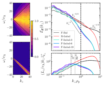
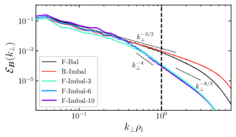
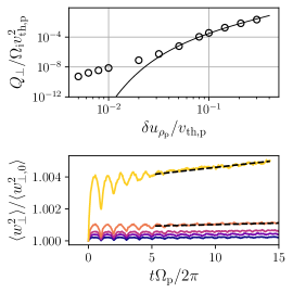
Results.—To highlight how imbalance affects the frequency spectrum of fluctuations, which was argued above to be important for controlling the heating, the left-hand plot of Fig. 1 shows the space-time Fourier transform , with ; here, denotes an average over all . In balanced turbulence, has significant power at small , a signature that the nonlinear and linear times are comparable [46]. In contrast, imbalanced turbulence is dominated by fluctuations at a particular frequency, as seen by the band peaked around . These show that increasing imbalance reduces the nonlinear broadening of fluctuations relative to their linear frequency, causing the ion heating to transition from a SH-like to QLH-like mechanism.
The electric-field spectra and for different turbulence simulations are compared on the right of Fig. 1, where we compute from its spectrum: [54]. In contrast to the wide inertial range of the imbalanced RMHD simulation, FLR-MHD captures the transition from an Alfvén-wave to kinetic-Alfvén-wave cascade [16], with the electric-field specturm approaching a scaling at . The presence of a helicity barrier is clearly seen in the imbalanced FLR-MHD simulations via the steep drop in spectra at , as observed in the solar wind [55, 31] and previous simulations [25, 26, 27]. The steep spectral slope of the helicity barrier also causes to reach a maximum at scales. This maximum, and the corresponding spectral break in , shifts to larger scales as the energy grows in time.
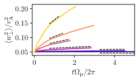
Figure 2 illustrates how the ion heating rate is calculated from the evolution of the ensemble-averaged perpendicular energy per unit mass for protons from with . Here is the component of , the thermal velocity of the protons after subtracting the local velocity, perpendicular to . Protons experience an initial heating transient lasting around one gyroperiod as they “pick up” the local velocity (also seen in Ref. [19]). Because of this, we calculate by a linear fit to via . Here is either the end of the simulation or when ; we choose this as decreases as increases [10, 19]. For , the initial heating transient exhibits oscillations, so to remove the effect of these from the measurement, we choose the start time for , for , and for (see Suppl. Mat.).
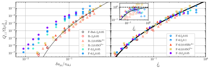
Figure 3 compares the dependence of on , the measure commonly used in SH theory, to our proposed definition . We calculate in Eq. (2) using from Fig. 1. It is clear that the standard normalization is inadequate for describing , particularly for cases with a helicity barrier. These show greater heating than expected from the power in fluctuations at these scales, indicating the true is being underestimated. Minor ions show similar heating rates in both imbalanced FLR-MHD and RMHD, due to their gyroradii lying at scales larger than and close to or above . In contrast, when plotted against our proposed , the data are well described by Eq. (1) with best fit parameters (fits of individual simulations to Eq. (1) comparing and are listed in Table 1); our value of is smaller than previous test particle simulations [10, 19] but similar to recent hybrid-kinetic simulations [22]. That Eq. (1) holds despite the difference in simulation conditions, from turbulence that is balanced, imbalanced, with or without a helicity barrier, and for both protons and minor ions, helps verify our unified model of ion heating. We note that the worst argreement is seen for imbalanced RMHD, which is also unphysical, neglecting the effect of on the turbulence.
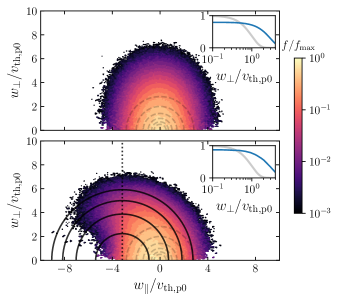
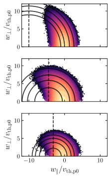
Despite the success of the unified model in reproducing , there remains important differences between balanced- and imbalanced-turbulent heating, as demonstrated in Fig. 4 which compares the proton velocity distribution functions (VDFs) in these two regimes. In balanced turbulence, the VDF undergoes diffusion in perpendicular velocity, as seen in the 1D VDF which has a characteristic flattopped shape [38, 22]. In contrast, in imbalanced turbulence the VDF diffuses along constant-energy contours within the frame of the waves, a hallmark of QLH [42]. For Alfvénic fluctuations, these contours are semicircles centered on the phase speed . The 1D VDF exhibits a flattopped shape similar to the balanced case (dropping off at slightly earlier upon close inspection), presumably because the contours are nearly vertical at small . This picture also allows an understanding of the -dependent dropoff in seen at large in Fig. 3 (representing the largest deviation from the phenomenological model): the constant-energy contours become increasingly curved as increases, where approaches , causing ions to gain parallel energy at the expense of perpendicular energy (see the Suppl. Mat.).
Conclusion.—In this Letter we provide a unified picture for describing ion heating in collisionless plasma turbulence across a wide range of regimes. The heating mechanism changes character depending on the frequency spectrum of turbulent fluctuations, transitioning from SH to QLH as the turbulence imbalance increases and reduces the relative nonlinear broadening of fluctuations. We propose a phenomenological model, controlled by the amplitude of fluctuations at the scale where peaks for , which accurately captures the ion-heating rate across both regimes. In the absence of a transition-range break or for minor ions, this scale is usually at and our model reduces to the standard SH formula; however, with a transition range, caused by the helicity barrier, this scale can lie above at . Using high-resolution simulations of test particles interacting with turbulence, we show that our proposal works well in describing measured heating rates for both protons and minor ions in turbulence that is balanced, imbalanced, with or without a helicity barrier. The fact that this holds, despite the very different ‘arced’ VDFs that result in imbalanced turbulence, hints at the universality of the heating mechanism.
We note that the FLR-MHD model, on which our results are based, is highly simplified, missing out the transition to ion-cyclotron waves when . Additionally, we also only measure the instantaneous ion from an initial Maxwellian, rather than tracking large changes of the velocity distribution function (as occurs for strong heating). Both of these issues have been addressed in a recent hybrid-kinetic study [56], which shows similar features. Nonetheless, the results of this Letter help to disentangle the signatures of ion heating and provide a base for more complex theories. The ideas presented here can also be used to understand helicity-barrier saturation on ion heating [26, 27], which is not captured by FLR-MHD and may be important for ab-initio models of coronal and solar-wind heating.
The authors would like to thank T. Adkins, B. D. G. Chandran, M. W. Kunz, N. F. Loureiro, M. Zhang, and M. Zhou for helpful discussions over the course of this work. Research is supported by the University of Otago, through a University of Otago Doctoral Scholarship (ZJ), and the Royal Society Te Apārangi, through Marsden-Fund grant MFP-UOO2221 (JS) and MFP-U0020 (RM), as well as through the Rutherford Discovery Fellowship RDF-U001004 (JS). High-performance computing resources were provided by the New Zealand eScience Infrastructure (NeSI) under project grant uoo02637.
References
- Marsch et al. [1982] E. Marsch, K.-H. Mühlhäuser, R. Schwenn, H. Rosenbauer, W. Pilipp, and F. M. Neubauer, Solar wind protons: Three-dimensional velocity distributions and derived plasma parameters measured between 0.3 and 1 AU, J. Geophys. Res. 87, 52 (1982).
- Marsch [2004] E. Marsch, On the temperature anisotropy of the core part of the proton velocity distribution function in the solar wind, J. Geophys. Res. 109, 10.1029/2003ja010330 (2004).
- Hellinger et al. [2006] P. Hellinger, P. Trávníček, J. C. Kasper, and A. J. Lazarus, Solar wind proton temperature anisotropy: Linear theory and wind/swe observations, Geophys. Res. Lett. 33, 10.1029/2006gl025925 (2006).
- Kohl et al. [1998] J. L. Kohl, G. Noci, E. Antonucci, G. Tondello, M. C. E. Huber, S. R. Cranmer, L. Strachan, A. V. Panasyuk, L. D. Gardner, M. Romoli, S. Fineschi, D. Dobrzycka, J. C. Raymond, P. Nicolosi, O. H. W. Siegmund, D. Spadaro, C. Benna, A. Ciaravella, S. Giordano, S. R. Habbal, M. Karovska, X. Li, R. Martin, J. G. Michels, A. Modigliani, G. Naletto, R. H. O’Neal, C. Pernechele, G. Poletto, P. L. Smith, and R. M. Suleiman, UVCS/SOHO empirical determinations of anisotropic velocity distributions in the solar corona, Astrophys. J. 501, L127 (1998).
- Esser et al. [1999] R. Esser, S. Fineschi, D. Dobrzycka, S. R. Habbal, R. J. Edgar, J. C. Raymond, J. L. Kohl, and M. Guhathakurta, Plasma properties in coronal holes derived from measurements of minor ion spectral lines and polarized white light intensity, Astrophys. J. 510, L63 (1999).
- Antonucci [2000] E. Antonucci, Fast solar wind velocity in a polar coronal hole during solar minimum, Solar Phys. 197, 115 (2000).
- Cranmer et al. [2009] S. R. Cranmer, W. H. Matthaeus, B. A. Breech, and J. C. Kasper, Empirical constraints on proton and electron heating in the fast solar wind, Astrophys. J. 702, 1604 (2009).
- Howes [2010] G. Howes, A prescription for the turbulent heating of astrophysical plasmas, Monthly Notices of the Royal Astronomical Society: Letters 409, L104 (2010), 1009.4212 .
- Kawazura et al. [2019] Y. Kawazura, M. Barnes, and A. A. Schekochihin, Thermal disequilibration of ions and electrons by collisionless plasma turbulence, Proc. Natl. Acad. Sci. U. S. A. 116, 771 (2019).
- Chandran et al. [2010] B. D. G. Chandran, B. Li, B. N. Rogers, E. Quataert, and K. Germaschewski, Perpendicular ion heating by low-frequency Alfvén-wave turbulence in the solar wind, Astrophys. J. 720, 503 (2010).
- Chandran et al. [2013] B. D. G. Chandran, D. Verscharen, E. Quataert, J. C. Kasper, P. A. Isenberg, and S. Bourouaine, Stochastic heating, differential flow, and the alpha-to-proton temperature ratio in the solar wind, ApJ 776, 45 (2013).
- Hollweg and Isenberg [2002] J. V. Hollweg and P. A. Isenberg, Generation of the fast solar wind: A review with emphasis on the resonant cyclotron interaction, Journal of Geophysical Research: Space Physics 107, SSH 12 (2002).
- Isenberg and Vasquez [2011] P. A. Isenberg and B. J. Vasquez, A kinetic model of solar wind generation by oblique ion-cyclotron waves, ApJ 731, 88 (2011).
- Isenberg and Vasquez [2019] P. A. Isenberg and B. J. Vasquez, Perpendicular ion heating by cyclotron resonant dissipation of turbulently generated kinetic Alfvén waves in the solar wind, Astrophys. J. 887, 63 (2019).
- Chandran [2005] B. D. G. Chandran, Weak compressible magnetohydrodynamic turbulence in the solar corona, Phys. Rev. Lett. 95, 265004 (2005).
- Schekochihin et al. [2009] A. A. Schekochihin, S. C. Cowley, W. Dorland, G. W. Hammett, G. G. Howes, E. Quataert, and T. Tatsuno, Astrophysical gyrokinetics: kinetic and fluid turbulent cascades in magnetized weakly collisional plasmas, Astrophys. J. Supp. 182, 310 (2009).
- TenBarge and Howes [2013] J. M. TenBarge and G. G. Howes, Current sheets and collisionless damping in kinetic plasma turbulence, ApJL 771, L27 (2013).
- Lehe et al. [2009] R. Lehe, I. J. Parrish, and E. Quataert, The heating of test particles in numerical simulations of Alfvénic turbulence, Astrophys. J. 707, 404 (2009).
- Xia et al. [2013] Q. Xia, J. C. Perez, B. D. G. Chandran, and E. Quataert, Perpendicular ion heating by reduced magnetohydrodynamic turbulence, Astrophys. J. 776, 90 (2013).
- Teaca et al. [2014] B. Teaca, M. S. Weidl, F. Jenko, and R. Schlickeiser, Acceleration of particles in imbalanced magnetohydrodynamic turbulence, Phys. Rev. E Stat. Nonlin. Soft Matter Phys. 90, 021101 (2014).
- Arzamasskiy et al. [2019] L. Arzamasskiy, M. W. Kunz, B. D. G. Chandran, and E. Quataert, Hybrid-kinetic simulations of ion heating in Alfvénic turbulence, Astrophys. J. 879, 53 (2019).
- Cerri et al. [2021] S. S. Cerri, L. Arzamasskiy, and M. W. Kunz, On stochastic heating and its phase-space signatures in low-beta kinetic turbulence, Astrophys. J. 916, 120 (2021).
- Weidl et al. [2015] M. S. Weidl, F. Jenko, B. Teaca, and R. Schlickeiser, Cosmic-ray pitch-angle scattering in imbalanced MHD turbulence simulations, ApJ 811, 8 (2015).
- Howes [2024] G. G. Howes, The fundamental parameters of astrophysical plasma turbulence and its dissipation: Nonrelativistic limit, arXiv [astro-ph.SR] (2024), arXiv:2402.12829 [astro-ph.SR] .
- Meyrand et al. [2021] R. Meyrand, J. Squire, A. A. Schekochihin, and W. Dorland, On the violation of the zeroth law of turbulence in space plasmas, J. Plasma Phys. 87, 10.1017/S0022377821000489 (2021).
- Squire et al. [2022] J. Squire, R. Meyrand, M. W. Kunz, L. Arzamasskiy, A. A. Schekochihin, and E. Quataert, High-frequency heating of the solar wind triggered by low-frequency turbulence, Nature Astronomy 6, 715 (2022).
- Squire et al. [2023] J. Squire, R. Meyrand, and M. W. Kunz, Electron–ion heating partition in imbalanced solar-wind turbulence, Astrophys. J. Lett. 957, L30 (2023).
- Schekochihin et al. [2019] A. A. Schekochihin, Y. Kawazura, and M. A. Barnes, Constraints on ion versus electron heating by plasma turbulence at low beta, J. Plasma Phys. 85, 10.1017/S0022377819000345 (2019).
- Goldreich and Sridhar [1995] P. Goldreich and S. Sridhar, Toward a theory of interstellar turbulence. 2: Strong Alfvénic turbulence, Astrophys. J. 438, 763 (1995).
- Leamon et al. [1998] R. J. Leamon, C. W. Smith, N. F. Ness, W. H. Matthaeus, and H. K. Wong, Observational constraints on the dynamics of the interplanetary magnetic field dissipation range, Journal of Geophysical Research: Space Physics 103, 4775 (1998).
- Bowen et al. [2020] T. A. Bowen, A. Mallet, S. D. Bale, J. W. Bonnell, A. W. Case, B. D. G. Chandran, A. Chasapis, C. H. K. Chen, D. Duan, T. Dudok de Wit, K. Goetz, J. S. Halekas, P. R. Harvey, J. C. Kasper, K. E. Korreck, D. Larson, R. Livi, R. J. MacDowall, D. M. Malaspina, M. D. McManus, M. Pulupa, M. Stevens, and P. Whittlesey, Constraining ion-scale heating and spectral energy transfer in observations of plasma turbulence, Phys. Rev. Lett. 125, 025102 (2020).
- Bowen et al. [2022] T. A. Bowen, B. D. G. Chandran, J. Squire, S. D. Bale, D. Duan, K. G. Klein, D. Larson, A. Mallet, M. D. McManus, R. Meyrand, J. L. Verniero, and L. D. Woodham, In situ signature of cyclotron resonant heating in the solar wind, Phys. Rev. Lett. 129, 165101 (2022).
- Bowen et al. [2024] T. A. Bowen, S. D. Bale, B. D. G. Chandran, A. Chasapis, C. H. K. Chen, T. Dudok de Wit, A. Mallet, R. Meyrand, and J. Squire, Mediation of collisionless turbulent dissipation through cyclotron resonance, Nat. Astron. , 1 (2024).
- McChesney et al. [1987] J. M. McChesney, R. A. Stern, and P. M. Bellan, Observation of fast stochastic ion heating by drift waves, Phys. Rev. Lett. 59, 1436 (1987).
- Johnson and Cheng [2001] J. R. Johnson and C. Z. Cheng, Stochastic ion heating at the magnetopause due to kinetic Alfvén waves, Geophys. Res. Lett. 28, 4421 (2001).
- Hoppock et al. [2018] I. W. Hoppock, B. D. G. Chandran, K. G. Klein, A. Mallet, and D. Verscharen, Stochastic proton heating by kinetic-Alfvén-wave turbulence in moderately high- plasmas, J. Plasma Phys. 84, 10.1017/S0022377818001277 (2018).
- Bourouaine and Chandran [2013] S. Bourouaine and B. D. G. Chandran, Observational test of stochastic heating in low- fast-solar-wind streams, ApJ 774, 96 (2013).
- Klein and Chandran [2016] K. G. Klein and B. D. G. Chandran, Evolution of the proton velocity distribution due to stochastic heating in the near-sun solar wind, Astrophys. J. 820, 47 (2016).
- Vech et al. [2017] D. Vech, K. G. Klein, and J. C. Kasper, Nature of stochastic ion heating in the solar wind: Testing the dependence on plasma beta and turbulence amplitude, Astrophys. J. Lett. 850, L11 (2017).
- Martinović et al. [2019] M. M. Martinović, K. G. Klein, and S. Bourouaine, Radial evolution of stochastic heating in low- solar wind, ApJ 879, 43 (2019).
- Martinović et al. [2020] M. M. Martinović, K. G. Klein, J. C. Kasper, A. W. Case, K. E. Korreck, D. Larson, R. Livi, M. Stevens, P. Whittlesey, B. D. G. Chandran, B. L. Alterman, J. Huang, C. H. K. Chen, S. D. Bale, M. Pulupa, D. M. Malaspina, J. W. Bonnell, P. R. Harvey, K. Goetz, T. Dudok de Wit, and R. J. MacDowall, The enhancement of proton stochastic heating in the near-Sun solar wind, Astrophys. J. Suppl. Ser. 246, 30 (2020).
- Kennel and Engelmann [1966] C. F. Kennel and F. Engelmann, Velocity space diffusion from weak plasma turbulence in a magnetic field, Phys. Fluids 9, 2377 (1966).
- Stix [1992] T. H. Stix, Waves in Plasmas, 1992nd ed. (American Institute of Physics, New York, NY, 1992).
- Schlickeiser and Achatz [1993] R. Schlickeiser and U. Achatz, Cosmic-ray particle transport in weakly turbulent plasmas. part 1. theory, J. Plasma Phys. 49, 63 (1993).
- Chen et al. [2001] L. Chen, Z. Lin, and R. White, On resonant heating below the cyclotron frequency, Phys. Plasmas 8, 4713 (2001).
- Schekochihin [2022] A. A. Schekochihin, MHD turbulence: a biased review, J. Plasma Phys. 88, 155880501 (2022).
- Lithwick et al. [2007] Y. Lithwick, P. Goldreich, and S. Sridhar, Imbalanced strong MHD turbulence, Astrophys. J. 655, 269 (2007).
- Beresnyak and Lazarian [2008] A. Beresnyak and A. Lazarian, Strong imbalanced turbulence, Astrophys. J. 682, 1070 (2008).
- Chandran [2000] B. D. Chandran, Scattering of energetic particles by anisotropic magnetohydrodynamic turbulence with a Goldreich-Sridhar power spectrum, Phys. Rev. Lett. 85, 4656 (2000).
- Passot et al. [2018] T. Passot, P. L. Sulem, and E. Tassi, Gyrofluid modeling and phenomenology of low- Alfvén wave turbulence, Phys. Plasmas 25, 042107 (2018).
- Strauss [1976] H. R. Strauss, Nonlinear, three-dimensional magnetohydrodynamics of noncircular tokamaks, Phys. Fluids 19, 134 (1976).
- Boldyrev et al. [2013] S. Boldyrev, K. Horaites, Q. Xia, and J. C. Perez, Toward a theory of astrophysical plasma turbulence at subproton scales, Astrophys. J. 777, 41 (2013).
- Teaca et al. [2009] B. Teaca, M. K. Verma, B. Knaepen, and D. Carati, Energy transfer in anisotropic magnetohydrodynamic turbulence, Phys. Rev. E Stat. Nonlin. Soft Matter Phys. 79, 046312 (2009).
- Bott et al. [2021] A. F. A. Bott, L. Arzamasskiy, M. W. Kunz, E. Quataert, and J. Squire, Adaptive critical balance and firehose instability in an expanding, turbulent, collisionless plasma, Astrophys. J. Lett. 922, L35 (2021).
- Kiyani et al. [2015] K. H. Kiyani, K. T. Osman, and S. C. Chapman, Dissipation and heating in solar wind turbulence: from the macro to the micro and back again, Philos. Trans. A Math. Phys. Eng. Sci. 373, 10.1098/rsta.2014.0155 (2015).
- Zhang et al. [2024] M. F. Zhang, M. W. Kunz, J. Squire, and K. G. Klein, Extreme heating of minor ions in imbalanced solar-wind turbulence, arXiv [astro-ph.SR] (2024), arXiv:2408.04703 [astro-ph.SR] .
- Howes et al. [2006] G. G. Howes, S. C. Cowley, W. Dorland, G. W. Hammett, E. Quataert, and A. A. Schekochihin, Astrophysical gyrokinetics: Basic equations and linear theory, Astrophys. J. 651, 590 (2006).
- Zocco and Schekochihin [2011] A. Zocco and A. A. Schekochihin, Reduced fluid-kinetic equations for low-frequency dynamics, magnetic reconnection, and electron heating in low-beta plasmas, Phys. Plasmas 18, 102309 (2011).
- Meyrand et al. [2019] R. Meyrand, A. Kanekar, W. Dorland, and A. A. Schekochihin, Fluidization of collisionless plasma turbulence, Proc. Natl. Acad. Sci. U. S. A. 116, 1185 (2019).
- David et al. [2024] V. David, S. Galtier, and R. Meyrand, Monofractality in the solar wind at electron scales: Insights from kinetic Alfvén waves turbulence, Phys. Rev. Lett. 132, 085201 (2024).
- Williamson [1980] J. H. Williamson, Low-storage Runge-Kutta schemes, J. Comput. Phys. 35, 48 (1980).
- Adkins et al. [2024] T. Adkins, R. Meyrand, and J. Squire, The effects of finite electron inertia on helicity-barrier-mediated turbulence, arXiv [physics.plasm-ph] (2024), arXiv:2404.09380 [physics.plasm-ph] .
- Mallet et al. [2017] A. Mallet, A. A. Schekochihin, and B. D. G. Chandran, Disruption of Alfvénic turbulence by magnetic reconnection in a collisionless plasma, J. Plasma Phys. 83, 905830609 (2017).
- Loureiro and Boldyrev [2017] N. F. Loureiro and S. Boldyrev, Collisionless reconnection in magnetohydrodynamic and kinetic turbulence, Astrophys. J. 850, 182 (2017).
- Zhou et al. [2023] M. Zhou, Z. Liu, and N. F. Loureiro, Electron heating in kinetic-Alfvén-wave turbulence, Proc. Natl. Acad. Sci. U. S. A. 120, e2220927120 (2023).
- Boris [1970] J. P. Boris, Relativistic plasma simulation-optimization, in Proc. Fourth Conf. Num. Sim. Plasmas (1970) pp. 3–67.
- Birdsall and Langdon [2018] C. K. Birdsall and A. B. Langdon, Plasma physics via computer simulation (CRC Press, 2018).
I Supplemental Material
The FLR-MHD Model
We use the finite Larmor radius MHD (FLR-MHD) model [50, 28, 25], a reduced fluid model that includes effects at scales both larger and smaller than without needing to solve kinetic equations. This theory can be derived from the Vlasov-Maxwell equations by assuming all quantities vary on timescales slower than the ion-cyclotron frequency, a strong background magnetic field, and that perturbations are elongated along magnetic field lines [57, 16]. Assuming a background magnetic field and taking the low- limit [58, 28] gives the equations of FLR-MHD:
| (3) | ||||
| (4) | ||||
| (5) |
where is the ratio of the ion and electron temperatures, is the perturbed electron density (equal to the ion density by quasi-neutrality), is the component of the magnetic vector potential, is the electrostatic potential, is the perpendicular flow, and is the magnetic field perturbation. The gyrokinetic Poisson operator , where is the modified Bessel function of the first kind and , models the transition from an Alfvénic to a kinetic-Alfvén-wave cascade that occurs at . In our simulations a hyperdiffusion operator (and similarly for ) is used to dissipate energy above grid scales, but does not model any specific physical process; we set in all cases except balanced FLR-MHD, discussed below.
This model describes the evolution of the Alfvénic component of turbulence both above and below ; the assumption of small leads to minimal coupling between this and the compressive component of the turbulence [16]. The FLR-MHD model is valid as long as the electron inertial length . This is because sets the length scale below which the magnetic field is no longer frozen into the electron flow; in this regime the equations are coupled to the electron distribution function and are no longer closed. Further details on the properties of FLR-MHD are given in Ref. [25].
Eigenmodes and Conserved Invarients
For a given wavenumber , the FLR-MHD model supports eigenmodes that travel parallel and anti-parallel to given by
| (6) |
with frequency . The normalized phase speed reduces to 1 at scales and is proportional to at scales, reflecting the transition from Alfvén to kinetic-Alfvén waves. These eigenmodes allow the definition of generalized Elsässer variables that reduce to the standard Elsässer variables of MHD () in the limit .
This model also has two conserved invariants: the free energy , and the generalized helicity . The helicity barrier results from the inability of the system to support a forward cascade of both and simultaneously at , due to the scaling in this range [25].
Additional Simulation Details
We use asterix [59, 25, 60], a modified verison of the pseudospectral code turbo [53], to solve the equations of RMHD and FLR-MHD, which are advanced in time with a third-order modified Williamson algorithm (a four-step, low-order Runge-Kutta method [61]). We force the imbalanced FLR-MHD and RMHD simulations with energy injection and , where is the ratio of the helicity and energy injection rates. In contrast, the balanced FLR-MHD simulation has no helicity injected into the system ().
Figure 5 shows the magnetic-field spectra of the high-resolution simulations after refinement (discussed below), corresponding to the electric-field spectra in Figure 1 of the Letter. All simulations exhibit an approximate scaling for . With the addition of a helicity barrier, the magnetic-field spectra show similar scalings to electric-field spectra, steeping to a scaling around .
Choice of Parallel Viscosity
We use different choices of the parallel viscosity in the different turbulent regimes to reflect how they arrive at a steady state. For imbalanced RMHD turbulence, the majority of the energy cascade is able to reach small perpendicular scales and dissipate there. However, due to critical balance this energy also reaches small parallel scales. To ensure correct dissipation at small scales, we use a non-zero parallel viscosity. For the helicity barrier, however, we are interested in how it affects the heating of test particles as it grows in time during the “pseudo-stationary” phase, before it saturates unphysically on the parallel hyperdissipation. We thus set for the helicity barrier simulation, studying it well before it would saturate with . Various tests (not shown) found that this produces results similar to using a non-zero .
Simulation Refinement
A highly imbalanced forcing causes the turbulence to take longer to reach a steady-state, as the energy cascade is less efficient for the stronger Elsässer field [47, 46]. The addition of a helicity barrier complicates this further as the system evolves through a “pseudo-stationary” state where the balanced portion of the cascade dissipates at small perpendicular scales, whereas the imbalanced portion grows at scales before saturating unphysically on parallel hyperdissipation [25, 26]. To run a high-resolution simulation, such as the ones used in this work, to this saturation point would be time-consuming and computationally expensive.
Instead, we start from simulations with a resolution of and let these evolve to a steady-state (or pseudo-stationary state for simulations with a helicity barrier). Once this point is reached, we refine the simulation by doubling the perpendicular resolution and decreasing the perpendicular viscosity , allowing the energy cascade to reach smaller scales before dissipating. Once the cascade has reached a new steady-state, we repeat this refinement procedure until the desired resolution is reached, which is then used as the starting point for our test particle simulations. The final resolutions are for the imbalanced RMHD and FLR-MHD cases, and for the balanced FLR-MHD case (the reason for this is discussed below).
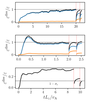
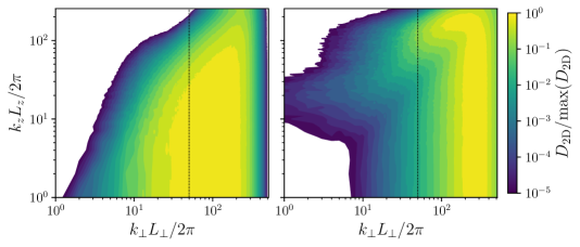
Figure 6 compares the time-evolution of dissipation in all balanced and imbalanced RMHD and FLR-MHD cases during the refinement process. The imbalanced cases take longer to saturate compared to the balanced case for the reason discussed above. As we increase the perpendicular resolution while refining the cascade can reach smaller corresponding parallel scales due to critical balance, leading to an increase in parallel dissipation. This effect is clearly seen in the balanced FLR-MHD case: the initial refinement in leads to an increase in , and the subsequent refinement in both and resulting in a decrease (due to dissipation scales occuring at larger ). In the imbalanced RMHD and balanced FLR-MHD cases, all energy is dissipated near the grid at predominately small perpendicular scales with . In contrast, the helicity barrier in the imbalanced FLR-MHD case blocks the majority of the cascade, only letting the balanced portion of the flux () through to be dissipated at grid scales; the remainder is “trapped” at large perpendicular scales. The lower-resolution simulations allow more of the cascade to be dissipated than predicted as their dissipation scales are close to -scales; this effect decreases as the range between these scales increases with resolution, as seen by the lower at each refinement level, converging to .
Figure 7 compares two-dimensional dissipation spectra from the high-resolution imbalanced FLR-MHD and RMHD simulations. In the absence of a helicity barrier, all energy is dissipated at grid scales in the RMHD case. In contrast, the presence of a helicity barrier causes a flat dissipation spectrum around , due to the steep energy spectrum slope in this range.
Viscosity in the Balanced FLR-MHD Case
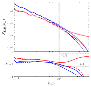
A notable exception to the methods described above was the balanced FLR-MHD turbulence case. Due to the transition from an Alfvénic to a kinetic-Alfvén-wave cascade at scales we expect the slope of the magnetic-field spectrum to steepen from to , and the electric-field specturm to flatten from to [62]. However, when refining the balanced FLR-MHD simulation to a resolution of with the method above we found that both the magnetic- and electric-field spectra were steeper than expected (dashed blue and red lines in Fig. 8, respectively), with the electric field reaching a slope of around . These spectra (solid lines in Fig. 8) approach their theoretical predictions after refining the simulation to a resolution of and switching off only the viscosity ( and ), leaving the electric field unaffected by dissipation (a method used in hybrid-kinetic simulations [21, 22, 26]). This steepening appears to be an unexpected nonlinear effect previously unseen in the FLR-MHD model. Previous work has shown that the reconnection of current sheets by sub- effects can lead to a steepening of the energy spectrum similar to what is seen in the transition range [63, 64, 65]; however, these require the electron inertial length which is ordered out of FLR-MHD. Whether what we observe here is related to this physics remains unclear, and more work is required to clarify the details of this mechanism. Because of this, we integrate particles using the balanced FLR-MHD simulation in the main Letter to remove any influence on heating due to this effect.
Additional Test Particle Details
In order to study particle heating, we introduced the ability to integrate test particles simultaneously with the fields solved by asterix. As in previous test particle simulations (e.g. [18, 19]), the equations of motion of the particles are integrated using the Boris push [66] with electric and magnetic fields interpolated from the grid to their positions via the triangular-shaped-cloud (TSC) method [18, 67]. The test particles are run simultaneously with the fluid code so that particles can use the current fields without needing to save the full history of the simulation. The perpendicular fields are obtained via and (with and as defined above via and in FLR-MHD); any artificial parallel electric field component due to interpolation is then removed using the method of Ref. [18]. We calculate the required timestep via [18], where is the fluid timestep calculated by asterix. Setting and was found to give accurate results; these results converge so long as (also seen by Ref. [18]).
There are some important differences between RMHD and FLR-MHD that need to be taken into account when implementing test particles. Firstly, the initial of the particle distribution is no longer a free parameter due to the inclusion of kinetic scales in the FLR-MHD model (in comparison to RMHD, which assumes ). We fix this parameter during the initialization of particles in an FLR-MHD simulation. Secondly, the inclusion of scales introduces a electric field component parallel to that arises from the conservation of magnetic flux in gyrokinetics [16, 22], given by
where is the unit vector along . We include this term when interpolating fields to the particles, although it is generally small in comparison to .
Testing of Implementation
After its implementation, the particle code was extensively tested to verify its correctness. Simple cases with known analytical properties (such as motion in constant and fields as well as conservation of energy in fields) are reproduced with a relative error of less than . The implementation of the TSC interpolation scheme was found to exhibit second-order convergence up to a resolution of , before additional errors dominate (e.g., from timestepping). The accuracy of this scheme was tested by comparing the use of grid-interpolated fields to those at the particle position via more complicated analytical fields (such as a linear combination of sinusoidal electromagnetic modes); for a grid resolution of or greater, the maximum relative error in energy evolution is less than .
The convergence of statistics with particle number was tested by running cohorts of particles (with ranging from 100 to in powers of 10) in the same balanced RMHD turbulence simulation. The relative error in the statistics of an and run is ; we use particles to allow for better statistics when calculating the velocity distribution functions.
Particle Heating at Small Turbulent Amplitudes
Ions experience a greater-than-expected heating rate than the empirical exponential suppression in (Eq. 1 of Letter) when initialized with very low . In Figure 9 we compare the measured heating rates of protons with interacting with the same balanced FLR-MHD turbulence simulation as those with ( from the main Letter). Due to the low-amplitude turbulence at -scales, the evolution of for these protons exhibits oscillations from the large-scale flow that introduces some ambiguity in measuring the heating rate; these oscillations are reduced with increasing as they experience greater heating (e.g., Figure 2 of the main Letter). We find that the oscillations decay after gyroperiods for ions initialized with , for those with , and for those with . To remove any contributions from the oscillations when measuring the linear growth of , we choose the start time of the linear fit for to be , , and gyroperiods respectively for the above cases (with the quarter-gyroperiod offset ensuring we are in the middle of any further oscillation cycle). Despite this, the measured heating rate is greater than that expected by exponential suppression ( for ).
Beta-dependent Perpendicular Heating in Imbalanced FLR-MHD Turbulence
In Fig. 10, we show how the diffusion of the proton velocity distribution function in imbalanced FLR-MHD turbulence depends on . Quasi-linear theory predicts that the evolution of the distribution function is a diffusion along constant-energy contours
| (7) |
within the frame of the dominant waves that the ions interact with [42, 43]. In Fig. 10, these are circles centred on the phase speed of Alfvénic fluctuations parallel to the magnetic field. At smaller , the contours of are nearly vertical for ions with small , with diffusion then leading to an increase in perpendicular energy and a greater measured heating rate (as seen in Figure 3 of the Letter).