A two-way heterogeneity model for dynamic networks
Abstract
Dynamic network data analysis requires joint modelling individual snapshots and time dynamics. This paper proposes a new two-way heterogeneity model towards this goal. The new model equips each node of the network with two heterogeneity parameters, one to characterize the propensity of forming ties with other nodes and the other to differentiate the tendency of retaining existing ties over time. Though the negative log-likelihood function is non-convex, it is locally convex in a neighbourhood of the true value of the parameter vector. By using a novel method of moments estimator as the initial value, the consistent local maximum likelihood estimator (MLE) can be obtained by a gradient descent algorithm. To establish the upper bound for the estimation error of the MLE, we derive a new uniform deviation bound, which is of independent interest. The usefulness of the model and the associated theory are further supported by extensive simulation and the analysis of some real network data sets.
Keywords: Degree heterogeneity, Dynamic networks, Maximum likelihood estimation, Uniform deviation bound
1 Introduction
Network data featuring prominent interactions between subjects arise in various areas such as biology, economics, engineering, medicine, and social sciences [27, 20]. As a rapidly growing field of active research, statistical modelling of networks aims to capture and understand the linking patterns in these data. A large part of the literature has focused on examining these patterns for canonical, static networks that are observed at a single snapshot. Due to the increasing availability of networks that are observed multiple times, models for dynamic networks evolving in time are of increasing interest now. These models typically assume, among others, that networks observed at different time are independent [28, 1], independent conditionally on some latent processes [4, 23], or drawn sequentially from an exponential random graph model conditional on the previous networks [11, 10, 21].
One of the stylized facts of real-life networks is that their nodes often have different tendencies to form ties and may evolve differently over time. The former is manifested by the fact that the so-called hub nodes have many links while the peripheral nodes have small numbers of connections in, for example, a big social network. The latter becomes evident when some individuals are more active in seeking new ties/friends than the others. In this paper, we refer to these two kinds of heterogeneity as static heterogeneity and dynamic heterogeneity respectively. Also known as degree heterogeneity in the static network literature, static heterogeneity has featured prominently in several popular models widely used in practice including the stochastic block model and its degree-corrected generalization [17]. See also [15, 29, 16, 19], and the references therein. Another common and natural approach to capture the static heterogeneity is to introduce node-specific parameters, one for each node. For single networks, this is often conducted via modelling the logit of the link probability between each pair of nodes as the sum of their heterogeneity parameters. Termed as the -model [2], this model and its generalizations have been extensively studied when a single static network is observed [39, 18, 7, 35, 3, 30].
With observed networks each having nodes, the goal of this study is two-fold: (i) We propose a dynamic network model named the two-way heterogeneity model that captures both static heterogeneity and dynamic heterogeneity, and develop the associate inference methodology; (ii) We establish new generic asymptotic results that can be applied or extended to different models with a large number of parameters (in relation to ). We focus on the scenario that the number of nodes goes to infinity. Our asymptotic results hold when , though may be fixed. The main contributions of our paper can be summarized as follows.
-
•
We introduce a reparameterization of the general autoregressive network model [14] to accommodate variations in both node degree and dynamic fluctuations. This novel approach can be regarded as an extension of the -model [2] to a dynamic framework. It encompasses two sets of parameters for heterogeneity: one governs static variations, akin to those in the standard -model, while the other addresses dynamic fluctuations. Unlike the general model in [14], which necessitates a large number of network observations (i.e. ), we demonstrate the validity of our formulation even in scenarios where is small but is large.
-
•
The formulation of our model gives rise to a high-dimensional non-convex loss function based on likelihood. By establishing the local convexity of the loss function in a neighborhood of the true parameters, we compute the local MLE by a standard gradient descent algorithm using a newly proposed method of moments estimator (MME) as its initial value. To our best knowledge, this is the first result in network data analysis for solving such a non-convex optimization problem with algorithmic guarantees.
-
•
Furthermore, to characterize the local MLE, we have derived its estimation error bounds in the norm and the norm when in which can be finite. Due to the dynamic structure of the data, the Hessian matrix of the loss function exhibits a complex structure. As a result, existing analytical approaches, such as the interior point theorem [6, 37] developed for static networks, are no longer applicable; see Section 3.1 for further elaboration. We derive a novel locally uniform deviation bound in a neighborhood of the true parameters with a diverging radius. Based on this we first establish norm consistency of the MLE, which paves the way for the uniform consistency in norm.
-
•
In establishing the locally uniform deviation bound, we have provided a general result for functions of the form as defined in (4.11) below. This result explores the sparsity structure of in the sense that most of its higher order derivatives are zero – the condition which our model satisfies, and provides a new bound that substantially extends the scope of empirical processes for the M-estimators [32] for the models with a fixed number of parameters to those with a growing number of parameters. The result here is of independent interest as it can be applied to any model with an objective function taking the form of .
The rest of the paper is organized as follows. We introduce in Section 2 the new two-way heterogeneity model and present its properties. The estimation of its local MLE in a neighborhood of the truth and the associated theoretical properties are presented in Section 3. The development of these properties relies on new local deviation bounds which are presented in Section 4. Simulation studies and an analysis of ants interaction data are reported in Section 5. We conclude the paper in Section 6. All technical proofs are relegated to Appendix A. Additional numerical results showcasing the effectiveness of our method in aiding community detection within stochastic block structures, along with an application aimed at understanding dynamic protein-protein interaction networks, are provided in Appendix B.
2 Two-way Heterogeneity Model
Consider a dynamic network defined on nodes which are unchanged over time. Denote by a matrix its adjacency matrix at time , i.e. indicates the existence of a connection between nodes and at time , and 0 otherwise. We focus on undirected networks without self-loops, i.e., for all , and for , though our approach can be readily extended to directed networks.
To capture the autoregressive pattern in dynamic networks, [14] proposed to model the network process via the following stationary AR(1) framework:
where denotes the indicator function, and the , are independent innovations satisfying
for some positive parameters and . This general model opts to neglect the inherent nature of the networks and chooses to estimate each pair independently. As a result, there are parameters and consistent model estimation requires . Conversely, in numerous real-world scenarios, it is frequently noted that the number of network observations is modest, while the number of nodes can significantly exceed . Under such a scenario of small--large-, the conventional model outlined in [14] may not be suitable. To address this and to effectively capture node heterogeneity in dynamic networks, as well as accommodate small--large- networks, we propose the following reparameterization for the general AR(1) model mentioned above. This reparameterization not only accounts for inherent node heterogeneity but also reduces the parameter count from to .
Definition 1.
Two-way Heterogeneity Model (TWHM). The data generating process satisfies
| (2.1) |
where the , for and are independent innovations with their distributions satisfying
| (2.2) |
TWHM defined above is a reparametrization of the AR(1) network model [14] as it reduces the total number of parameters from therein to . By Proposition 1 of [14], the matrix process is strictly stationary with
| (2.3) |
provided that we activate the process with also following this stationary marginal distribution.
Furthermore,
| (2.4) |
Note that the connection probabilities in (2.3) depend on only, and are of the same form as the (static) -model [2]. Hence we call the static heterogeneity parameter. Proposition 1 below confirms that means and variances of node degrees in TWHM also depend on only, and that different values of reflect the heterogeneity in the degrees of nodes.
Under TWHM, it holds that
| (2.5) |
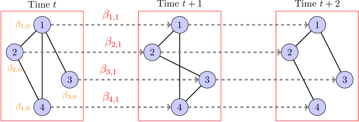
Hence the dynamic changes (over time) of network depend on, in addition to , : the larger is, the more likely will retain the value of for all . Thus we call the dynamic heterogeneity parameter, as its components reflect the different dynamic behaviours of the nodes. A schematic description of the model can be seen from Figure 1 where three snapshots of a dynamic network with four nodes are depicted.
From now on, let denote the stationary TWHM with parameters , and be the degree of node at time . The proposition below lists some properties of the node degrees.
Proposition 1.
Let . Then is a strictly stationary process. Furthermore for any and ,
where .
Proposition 1 implies that when there exist constants and such that and for all , the degree sequence is approximately AR(1).
3 Parameter Estimation
We introduce some notation first. Denote by the identity matrix. For any , denotes the vector with all its elements equal to . For and , let for any , , and . Furthermore, let denote the spectral norm of which equals its largest eigenvalue. For a random matrix with , define its matrix variance as . The notation means that there exists a constant such that , while notation means there exists a constant such that . Denote by the ball centred at with radius . Let denote some generic constants that may be different in different places. Let be the true unknown parameters. We assume:
-
(A1)
There exists a constant such that for any , the true parameters satisfy .
Condition (A1) ensures that the autocorrelation functions (ACFs) in (2.4) are bounded away from 1 for any . It is worth noting that both and are allowed to vary with , thus accommodating sparse networks in our analysis. In practical terms, , which reflects the sparsity of the stationary network, tends to be very small for large networks. Consequently, condition (A1) holds when is bounded from above.
3.1 Maximum likelihood estimation
With the available observations , the log-likelihood function conditionally on is of the form . Note for different are independent with each other. By (2.5), a (normalized) negative log-likelihood admits the following form:
| (3.6) | ||||
For brevity, write
| (3.7) |
Then the Hessian matrix of is of the form
where for ,
Note that matrix is symmetric. Furthermore, the three matrices and are diagonally balanced [12] in the sense that their diagonal elements are the sums of their respective rows, namely,
Unfortunately the Hessian matrix is not uniformly positive-definite. Hence is not convex; see Section 5.1 for an example. Therefore, finding the global MLE by minimizing would be infeasible, especially given the large dimensionality of . To overcome the obstacle, we propose the following roadmap to search for the local MLE over a neighbourhood of the true parameter values .
-
(1)
First we show that is locally convex in a neighbourhood of (see Theorem 1 below). Towards this end, we first prove that is positive definite in a neighborhood of . Leveraging on some newly proved concentration results, we show that converges to uniformly over the neighborhood.
-
(2)
Denote by the local MLE in the neighbourhood identified above. We derive the bounds for respectively in both and norms (see Theorems 2 and 3 below). The convergence is established by providing a uniform upper bound for the local deviation between and (see Corollary 4 in Section 4). The convergence of is established by further exploiting the special structure of the objective function.
-
(3)
We propose a new method of moments estimator (MME) which is proved to lie asymptotically in the neighbourhood specified in (1) above. With this MME as the initial value, the local MLE can be simply obtained via a gradient decent algorithm.
The main technical challenges in the roadmap above can be summarized as follows.
Firstly, to establish the upper bounds as stated in (2) above, we need to evaluate the uniform local deviations of the loss function. While the theoretical framework for deriving similar deviations of M-estimators has been well established in, for example, [32, 31], classical techniques in empirical process for establishing uniform laws [33] are not applicable because the number of parameters in TWHM diverges.
Secondly, for the classical -model, proving the existence and convergence of its MLE relies strongly on the interior point theorem [6]. In particular, this theorem is applicable only because the Hessian matrix of the -model admits a nice structure, i.e. it is diagonally dominant and all its elements are positive depending on the parameters only [2, 39, 37, 8]. However the Hessian matrix of for TWHM depends on random variables ’s in addition to the parameters, making it impossible to verify if the score function is uniformly Fréchet differentiable or not, a key assumption required by the interior point theorem.
Lastly, the higher order derivatives of may diverge as the order increases. To see this, notice that for any integer , the -th order derivatives of is closely related to the -th order derivatives of the Sigmoid function in that , where is the Eulerian number [26]. Some of the coefficients can diverge very quickly as increases. Thus, loosely speaking, is not smooth. This non-smoothness and the need to deal with a growing number of parameters make various local approximations based on Taylor expansions highly non-trivial; noting that the consistency of MLEs in many finite-dimensional models is often established via these approximations.
In our proofs, we have made great use of the special sparse structure of the loss function in the form (4.11) below. This sparsity structure stems from the fact that most of its higher order derivatives are zero. Based on the uniform local deviation bound obtained in Section 4, we have established an upper bound for the error of the local MLE under the norm. Utilizing the structure of the marginalized functions of the loss we have further established an upper bound for the estimation error under the norm thanks to an iterative procedure stated in Section 3.3.
3.2 Existence of the local MLE
To establish the convexity of in a neighborhood of , we first show that such a local convexity holds for .
Proposition 2.
Let be a matrix defined as where , , are symmetric matrices. Then is positive (negative) definite if are all positive (negative) definite.
Proof.
Consider any nonzero where , we have:
This proves the proposition. ∎
Noting that and are all diagonally balanced matrices, with some routine calculations it can be shown that and have only positive elements, and thus are all positive definite. Therefore, is positive definite by Proposition 2. By continuity, when is close enough to , is also positive definite, and hence is strongly convex in a neighborhood of . Next we want to show the local convexity of whose second order derivatives depend on the sufficient statistics , and . By noticing that the network process is -mixing with an exponential decaying mixing coefficient, we first obtain the following concentration results for and , which ensure element-wise convergence of to for a given when .
Lemma 1.
Suppose for some satisfying condition (A1). Then for any , is -mixing with exponential decaying rates. Moreover, for any positive constant , by choosing to be large enough, it holds with probability greater than that
where .
The following lemma provides a lower bound for the smallest eigenvalue of .
Lemma 2.
Let , and . Under condition (A1), for any and with being a small enough constant, there exists a constant such that
Examining the proof indicates that the lower bound in Lemma 2 is attained when and . Hence the smallest eigenvalue of can decay exponentially in and . Consequently, an upper bound for the radius and must be imposed so as to ensure the positive definiteness of the sample analog . Moreover, Lemma 2 also indicates that the positive definiteness of can be guaranteed when is within the ball . To establish the existence of the local MLE in the neighborhood, we need to evaluate the closeness of and in terms of the operator norm. Intuitively, for some appropriately chosen , if has a smaller order than uniformly over the parameter space and , the positive definiteness of can be concluded.
Note that and are all centered and diagonally balanced matrices which can be decomposed into sums of independent random matrices. The following lemma provides a bound for evaluating the moderate deviations of these centered matrices.
Lemma 3.
Let be a symmetric random matrix such that the off-diagonal elements are independent of each other and satisfy
Then it holds that
Theorem 1.
Let condition (A1) hold, assume , and where with for some small enough constant . Then as with , we have that, with probability tending to one, there exists a unique MLE in the ball for some , where is a constant.
In the proof of Theorem 1, we have shown that with probability tending to 1, is convex in the convex and closed set . Consequently, we conclude that there exists a unique local MLE in . From Theorem 1 we can also see that when becomes larger, the radius will be smaller, and when is bounded away from infinity, has a constant order. From the proof we can also see that the constant can be larger if the smallest eigenvalue of the expected Hessian matrix is larger. Further, by allowing the upper bound of to grow to infinity, our theoretical analysis covers the case where networks are sparse. Specifically, under the condition that , from (2) we can obtain the following lower bound (which is achievable when ) for the density of the stationary network:
In particular, when for some constant , we have . Thus, compared to full dense network processes where the total number of edges for each network is of the order , TWHM allows the networks with much fewer edges.
3.3 Consistency of the local MLE
In the previous subsection, we have proved that with probability tending to one, is convex in , where is defined in Theorem 1. Denote by the (local) MLE in . We now evaluate the and distances between and the true value .
Based on Theorem 5 we obtain a local deviation bound for as in Corollary 4 in Section 4, from which we establish the following upper bound for the estimation error of under the norm:
Theorem 2.
Let condition (A1) hold, assume , and where with for some small enough constant . Then as with , it holds with probability converging to one that
We discuss the implication of this theorem. When and is finite, that is, when we have a fixed number of nodes but a growing number of network snapshots, Theorem 2 indicates that when is small enough. On the other hand, when , and are finite, Theorem 2 indicates that as the number of parameters increases, the error bound of increases at a much slower rate .
Although Theorem 2 indicates that as , it does not guarantee the uniform convergence of all the elements in . To prove the uniform convergence in the norm, we exploit a special structure of the loss function and the norm bound obtained in Theorem 2. Specifically, denote in (3.6) as where , and contains the remaining elements of except . Using this notation, we can analogously define and for the true parameter , and and for the local MLE . We then have that is the mimizer of while is the minimizer of . The error of in estimating then relies on the distance between and , which on the other hand depends on both the bound of and the uniform local deviation bound of . Based on Theorem 2, Corollary 4 in Section 4, and a sequential approach (see equations (A.30) and (A.31) in the appendix), we obtain the following bound for the estimation error under the norm.
Theorem 3.
Let condition (A1) hold, assume , and where with for some small enough constant . Then as , it holds with probability converging to one that
Theorem 3 indicates that as . Thus all the components of converge uniformly. On the other hand, when for some small enough positive constant , we have . Compared with Theorem 1, we observe that although the radius in Theorem 1 already tends to zero when and for some small enough constant , the error bound of has a smaller order asymptotically and thus gives a tighter convergence rate.
We remark that in the MLE, and are estimated jointly. As we can see from the log-likelihood function, the information related to is captured by and , , while that related to is captured by and , . This indicates that the effective “sample sizes” for estimating and are both of the order . While the theorems we have established in this section is for jointly, we would expect and to have the same rate of convergence.
3.4 A method of moments estimator
Having established the existence of a unique local MLE in and proved its convergence, we still need to specify how to find this local MLE. To this end, we propose an initial estimator lying in this neighborhood. Consequently we can adopt any convex optimization method such as the coordinate descent algorithm to locate the local MLE, thanks to the convexity of the loss function in this neighborhood. Based on (2.3), an initial estimator of denoted as can be found by solving the following method of moments equations
| (3.8) |
These equations can be viewed as the score functions of the pseudo loss function . Since the Hessian matrix of is diagonally balanced with positive elements, the Hessian matrix is positive definite, and, hence, is strongly convex. With the strong convexity, the solution of (3.8) is the minimizer of which can be easily obtained using any standard algorithms such as the gradient descent. On the other hand, note that
which motivates the use of the following estimating equations to obtain , the initial estimator of ,
| (3.9) |
with . Similar to (3.8), we can formulate a pseudo loss function such that given , its Hessian matrix corresponding to the score equations (3.9) is positive definite, and hence (3.9) can also be solved via the standard gradient descent algorithm. Since is obtained by solving two sets of moment equations, we call it the method of moments estimator (MME). An interesting aspect of our construction of these moment equations is that the equations corresponding to the estimation of and are decoupled. While the estimator error in estimating propagates clearly in that of estimating , we have the following existence, uniqueness, and a uniform upper bound for the estimation error of . Our results build on a novel application of the classical interior mapping theorem [6, 38, 37].
Theorem 4.
When and are finite, Theorem 4 gives . When , we see that the upper bound for the local MLE in Theorem 3 is dominated by the upper bound of the MME in Theorem 4. Moreover, when for some small enough constant , we have , where is defined in Theorem 1. Thus, is in the small neighborhood of as required.
3.5 The sparse case
In the previous results, the estimation error bounds depend on and , i.e., the upper bounds on and . Clearly, the larger is, the more sparse the networks could be, and the larger is, the lag-one correlations (c.f. equation (2.4)) could be closer to one, indicating fewer fluctuations in the network process. To further characterize the effect of network sparsity, in this section, we derive further properties under a relatively sparse scenario where and for all and here is a constant. Under this case, there exist constants and such that In the most sparse case where , the density of the stationary network is of the order . Similar to Lemma 2 and Theorem 1, the following corollary provides a lower bound for the smallest eigenvalue of and the existence of the MLE.
Corollary 1.
Let , for some where is a small enough constant. Denote for some constant . Then, under condition (A1), there exists a constant such that
Further, assume that and for some positive constant . Then, as with , with probability tending to 1, there exists a unique MLE in .
Following Theorems 2-4, we also establish the estimation errors for the MLE and MME in the subsequent corollaries below.
Corollary 2.
Let condition (A1) hold. Assume , , and for , and some constant . Then as with , it holds with probability tending to one that
Corollary 3.
From Corollary 2, we can see that when , the MLE is consistent when for some positive constant , with the corresponding lower bound in the density as . Similarly, from Corollary 3 we can see that when , the density of the networks can be as small as for some constant , i.e., the density has a larger order than for the estimation of the MME. Further, when for some constant , we have , where is defined in Corollary 1. This implies the validity of using as an initial estimator for computing the local MLE.
4 A uniform local deviation bound under high dimensionality
As we have discussed, a key to establish the consistency of the local MLE is to evaluate the magnitude of for all with specified in Theorem 1. Such local deviation bounds are important for establishing error bounds for general M-estimators in the empirical processes [32]. Note that
| (4.10) | ||||
where and are defined in (3.7). The three terms on the right-hand side all admit the following form
| (4.11) |
for some functions , , and centered random variables . Instead of establishing the uniform bound for each term in (4.10) separately, below we will establish a unified result for bounding over a local ball defined as for a general function as in (4.11). We remark that in general without further assumptions on , establishing uniform deviation bounds is impossible when the dimension of the problem diverges. For our TWHM however, the decomposition (4.10) is of a particularly appealing structure in the sense that only two-way interactions between parameters exist. Based on this “sparsity” structure, we develop a novel reformulation (c.f. equation (A.15)) for the main components of the Taylor series of satisfying the following two conditions.
-
(L-A1)
There exists a constant , such that for any , any positive integer , and any non-negative integer , we have:
-
(L-A2)
Random variables are independent satisfying , and for any and , where and are constants depending on and but independent of and .
Loosely speaking, Condition (L-A1) can be seen as a smoothness assumption on the higher order derivatives of so that we can properly bound these derivatives when Taylor expansion is applied. On the other hand, the upper bound for these derivatives is mild as it can diverge very quickly as increases. For our TWHM, it can be verified that (L-A1) holds for and ; see (3.6). For the latter, note that the first derivative of function is seen as the Sigmoid function:
By the expression of the higher order derivatives of the Sigmoid function [26], the -th order derivative of is
where and is the Eulerian number. Now for any , we have
Therefore,
holds for all and . With extra arguments using the chain rule, this in return implies that (L-A1) is satisfied with when .
Condition (L-A2) is a regularization assumption for the random variables , and the bounds on their moments are imposed to ensure point-wise concentration. For our TWHM, from Lemma 1 and Lemma 5, we have that there exist large enough constants and such that with probability greater than , the random variables , and all satisfy condition (L-A2) with and .
We present the uniform upper bound on the deviation of below.
Theorem 5.
Assume conditions (L-A1) and (L-A2). For any given and , there exist large enough constants and which are independent of , such that, as , with probability greater than ,
holds uniformly for all .
One of the main difficulties in analyzing defined in (4.11) is that and are coupled, giving rise to complex terms involving both in the Taylor expansion of . When Taylor expansion with order is used, condition (L-A1) can reduce the number of higher order terms from to . On the other hand, by formulating the main terms in the Taylor series into a matrix form in (A.15), the uniform convergence of the sum of these terms is equivalent to that of the spectral norm of a centered random matrix, which is independent of the parameters. Further details can be found in the proofs of Theorem 5.
Define the marginal functions of as
by retaining only those terms related to . Similar to Theorem 5, we state the following upper bound for these marginal functions. With some abuse of notation, let be the vector containing all the elements in except .
Theorem 6.
If conditions (L-A1) and (L-A2) hold, then for any given and , there exist large enough constants and which are independent of , such that, as , with probability greater than ,
holds uniformly for all , and .
Similar to (4.10), we can also decompose into the sum of three components taking the form (4.11). Consequently, by setting in Theorems 5 and 6 to be the true parameter , we can obtain the following upper bounds.
Corollary 4.
For any given , there exist large enough positive constants and such that
-
(i)
with probability greater than ,
(4.12) holds uniformly for all with some constant ;
-
(ii)
with probability greater than ,
(4.13) holds uniformly for all with some constant .
In (4.12) and (4.13) we have replaced the norm based upper bounds in Theorems 5 and 6 with norm based upper bounds using the fact that for all , . It is recognized that networks often exhibit diverse characteristics, including dynamic changes, node heterogeneity, homophily, and transitivity, among others. In this paper, our primary emphasis is on addressing node heterogeneity within dynamic networks. When integrated with other stylized features, the objective function may adopt a similar structure to the function defined in Equation . Moreover, many other models that incorporate node heterogeneity can express their log-likelihood functions in a form analogous to Equation (4.11). For instance, the general category of network models with edge formation probabilities represented as , where is a density or probability mass function, and denote node-specific parameters for node . This encompasses models such as the model [13], the directed -model [36], and the bivariate gamma model [8]. Additionally, in the domain of ranking data analysis, it is common to introduce individual-specific parameters or scores for ranking, as observed in the classical Bradley-Terry model and its variants [9]. Our discoveries have the potential for application in the theoretical examination of these models or their modifications when considering additional stylized features alongside node heterogeneity.
5 Numerical study
In this section, we assess the performance of the local MLE. For comparison, we have also computed a regularized MME that is numerically more stable than the vanilla MME in (3.9). Specifically, for the former, we solve
| (5.14) |
with , where can be seen as a ridge penalty with as the regularization parameter. Denote the regularized MME as . Similar to Theorem 4, by choosing for some constant , we can show that In our implementation we take . The MLE of TWHM is obtained via gradient descent using as the initial value.
5.1 Non-convexity of and
Given the form of , it is intuitively true that it may not be convex everywhere. We confirm this via a simple example. Take and set to be , or . We evaluate the smallest eigenvalue of the Hessian matrix of and its expectation at the true parameter value , or at in one experiment.
| Sign of the smallest eigenvalue of | Sign of the smallest eigenvalue of | ||||||
|---|---|---|---|---|---|---|---|
| = | = | = | = | = | = | ||
| = | = | ||||||
| = | = | ||||||
| = | = | ||||||
| Sign of the smallest eigenvalue of | Sign of the smallest eigenvalue of | ||||||
| = | = | = | = | = | = | ||
| = | = | ||||||
| = | = | ||||||
| = | = | ||||||
From the top half of Table 1 we can see that, when evaluated at , the Hessian matrices are all positive definite. However, when evaluated at , from the bottom half of the table we can see that the Hessian matrices are no longer positive definite when is far away from . Even when the Hessian matrix of is so at with , the corresponding Hessian matrix of at this point has a negative eigenvalue. Thus, and are not globally convex.
5.2 Parameter estimation
We first evaluate the error rates of the MLE and MME under different combinations of and . We set or and , which results in a total of 28 different combinations of . For each , the data are generated such that where the parameters and () are drawn independently from the uniform distribution with parameters in . Each experiment is repeated 100 times under each setting. Denote the estimator (which is either the MLE or the MME) as , and the true parameter value as . We report the average error in terms of and the average error in Figure 2.
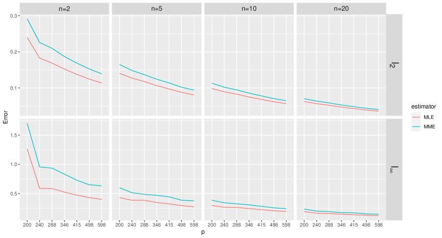
From this figure, we can see that the errors in terms of the norm and the norm decrease for MME and MLE as or increases, while the errors of MLE are smaller across all settings. These observations are consistent with our findings in the main theory.
Next, we provide more numerical simulation to evaluate the performance of MLE and MME by imposing different structures on and . In particular, we want to evaluate how the estimation accuracy changes by varying the sparsity of the networks as well as varying the correlations of the network sequence. Note that the expected density of the stationary distribution of the network process is simply
In the sequel, we will use two parameters and to generate , , according to the following four settings:
-
Setting 1.
: all the elements in are set to be equal to .
-
Setting 2.
: the first 10 elements of are set to be equal to , while the other elements are set to be equal to .
-
Setting 3.
: the parameters take values in a linear form as , .
-
Setting 4.
: the elements in are generated independently from the uniform distribution with parameters and .
In Table 2, we generate using Setting 1 with , and generate using Setting 2 with different choices for and to obtain networks with different expected density. In Table 3, we generate and using combinations of these four settings with different parameters such that the resulting networks have expected density either around 0.05 (sparse) or 0.5 (dense). The number of networks in each process and the number of nodes in each network are set as or . The errors for estimating in terms of the and norms are reported via 100 replications. To further compare the accuracy for estimating and , in Table 4, we have conducted experiments under Settings 3 and 4, and reported the estimation errors for and separately. We summarize the simulation results below:
| MME, | MME, | MLE, | MLE, | |||||
| 20 | 200 | {0} | 0.074 | 0.219 | 0.071 | 0.212 | ||
| 50 | 200 | {0} | 0.046 | 0.138 | 0.045 | 0.136 | ||
| 20 | 500 | {0} | 0.046 | 0.150 | 0.045 | 0.146 | ||
| 50 | 500 | {0} | 0.029 | 0.093 | 0.028 | 0.092 | ||
| 20 | 200 | 0.092 | 0.222 | 0.091 | 0.217 | |||
| 50 | 200 | 0.058 | 0.140 | 0.058 | 0.139 | |||
| 20 | 500 | 0.058 | 0.154 | 0.057 | 0.148 | |||
| 50 | 500 | 0.036 | 0.095 | 0.036 | 0.093 | |||
| 20 | 200 | 0.120 | 0.305 | 0.117 | 0.284 | |||
| 50 | 200 | 0.074 | 0.186 | 0.074 | 0.177 | |||
| 20 | 500 | 0.075 | 0.200 | 0.073 | 0.190 | |||
| 50 | 500 | 0.038 | 0.125 | 0.036 | 0.119 | |||
| 20 | 200 | 0.164 | 0.436 | 0.156 | 0.397 | |||
| 50 | 200 | 0.102 | 0.255 | 0.097 | 0.236 | |||
| 20 | 500 | 0.103 | 0.287 | 0.097 | 0.262 | |||
| 50 | 500 | 0.065 | 0.178 | 0.061 | 0.164 |
| Density = 0.05 | |||||||
|---|---|---|---|---|---|---|---|
| MME, | MME, | MLE, | MLE, | ||||
| 20 | 200 | 0.419 | 1.833 | 0.392 | 1.8 | ||
| 50 | 200 | 0.253 | 0.913 | 0.227 | 0.82 | ||
| 20 | 500 | 0.246 | 1.119 | 0.218 | 0.9 | ||
| 50 | 500 | 0.170 | 0.626 | 0.148 | 0.621 | ||
| 20 | 200 | {0} | 0.275 | 1.452 | 0.280 | 1.516 | |
| 50 | 200 | {0} | 0.161 | 0.771 | 0.162 | 0.774 | |
| 20 | 500 | {0} | 0.160 | 0.892 | 0.162 | 0.904 | |
| 50 | 500 | {0} | 0.098 | 0.506 | 0.099 | 0.507 | |
| 20 | 200 | 0.187 | 0.588 | 0.161 | 0.514 | ||
| 50 | 200 | 0.116 | 0.351 | 0.099 | 0.305 | ||
| 20 | 500 | 0.114 | 0.387 | 0.099 | 0.339 | ||
| 50 | 500 | 0.073 | 0.246 | 0.062 | 0.208 | ||
| 20 | 200 | {0} | 0.150 | 0.482 | 0.151 | 0.484 | |
| 50 | 200 | {0} | 0.93 | 0.289 | 0.093 | 0.29 | |
| 20 | 500 | {0} | 0.93 | 0.309 | 0.093 | 0.311 | |
| 50 | 500 | {0} | 0.058 | 0.195 | 0.058 | 0.195 | |
| Density = 0.5 | |||||||
| 20 | 200 | 0.132 | 0.415 | 0.012 | 0.318 | ||
| 50 | 200 | 0.080 | 0.238 | 0.069 | 0.194 | ||
| 20 | 500 | 0.080 | 0.272 | 0.068 | 0.217 | ||
| 50 | 500 | 0.050 | 0.168 | 0.043 | 0.135 | ||
| 20 | 200 | 0.107 | 0.324 | 0.095 | 0.264 | ||
| 50 | 200 | 0.067 | 0.194 | 0.060 | 0.163 | ||
| 20 | 500 | 0.071 | 0.267 | 0.061 | 0.205 | ||
| 50 | 500 | 0.044 | 0.156 | 0.039 | 0.130 | ||
| 20 | 200 | 0.137 | 0.478 | 0.112 | 0.329 | ||
| 50 | 200 | 0.084 | 0.274 | 0.070 | 0.205 | ||
| 20 | 500 | 0.087 | 0.352 | 0.071 | 0.250 | ||
| 50 | 500 | 0.054 | 0.211 | 0.044 | 0.150 | ||
| 20 | 100 | 20 | 100 | ||
| 200 | 200 | 500 | 500 | ||
| and | |||||
| MME, | 0.163(0.010) | 0.096(0.006) | 0.099(0.004) | 0.057(0.002) | |
| 0.177(0.010) | 0.084(0.005) | 0.104(0.004) | 0.050(0.002) | ||
| MME, | 0.570(0.103) | 0.367(0.085) | 0.395(0.070) | 0.241(0.042) | |
| 0.658(0.137) | 0.421(0.079) | 0.438(0.076) | 0.214(0.037) | ||
| MLE, | 0.211(0.013) | 0.091(0.006) | 0.121(0.005) | 0.054(0.002) | |
| 0.166(0.011) | 0.072(0.005) | 0.096(0.004) | 0.043(0.002) | ||
| MLE, | 0.809(0.180) | 0.354(0.076) | 0.532(0.098) | 0.232(0.041) | |
| 0.617(0.116) | 0.265(0.052) | 0.399(0.065) | 0.172(0.028) | ||
| and | |||||
| MME, | 0.133(0.012) | 0.080(0.007) | 0.081(0.004) | 0.047(0.002) | |
| 0.093(0.006) | 0.053(0.004) | 0.056(0.003) | 0.032(0.002) | ||
| MME, | 0.568(0.104) | 0.365(0.087) | 0.394(0.071) | 0.241(0.042) | |
| 0.387(0.069) | 0.236(0.043) | 0.258(0.037) | 0.162(0.025) | ||
| MLE, | 0.176(0.016) | 0.076(0.007) | 0.100(0.006) | 0.044(0.002) | |
| 0.116(0.009) | 0.051(0.004) | 0.068(0.003) | 0.031(0.002) | ||
| MLE, | 0.809(0.181) | 0.351(0.078) | 0.531(0.099) | 0.232(0.041) | |
| 0.513(0.088) | 0.227(0.047) | 0.348(0.058) | 0.158(0.024) | ||
-
•
The effect of . Similar to what we have observed in Figure 2, the estimation errors become smaller when or becomes larger. Interestingly, from Tables 2–3 we can observe that, under the same setting, the errors in norm when are very close to those when . This is to some degree consistent with our finding in Theorem 2 where the upper bound depends on through their product .
-
•
The effect of sparsity. From Table 2 we can see that, as the expected density decreases, the estimation errors increase in almost all the cases. On the other hand, even though the parameters take different values in Table 3, the errors in the sparse cases are in general larger than those in the dense cases.
- •
-
•
MLE vs MME. In general, the estimation errors of the MLE are smaller than those of the MME in most cases as can be seen in Tables 2 and Table 3. In Table 4 where the estimation errors for and are reported separately, we can see that the estimation errors of the MME of are generally larger than those of the MLE of , especially when is large.
5.3 Real data
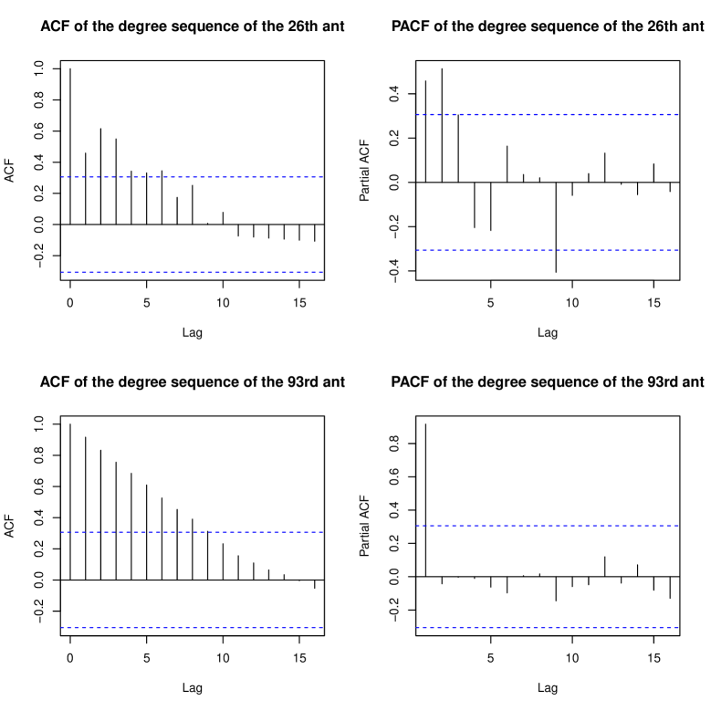
In this section, we apply our TWHM to a real dataset to examine an insect interaction network process [25]. We focus on a subset of the data named insecta-ant-colony4 that contains the social interactions of 102 ants in 41 days. In this dataset, the position and orientation of all the ants were recorded twice per second to infer their movements and interactions, based on which 41 daily networks were constructed. More specifically, is 1 if there is an interaction between ants and during day , and 0 otherwise. In the ACF and PACF plots of the degree sequences of selected ants (c.f. Figure 1 in Appendix B.1), we can observe patterns similar to those of a first-order autoregressive model with long memory. This motivates the use of TWHM for the analysis of this dataset.
In [25], the 41 daily networks were split into four periods with 11, 10, 10, and 10 days respectively, because the corresponding days separating these periods were identified as change-points. By excluding ants that did not interact with others, we are left with nodes in period one, nodes in period two, nodes in period three and nodes in period four. Thus we take the networks on day 1, day 12, day 22 and day 32 as the initial networks and fit four different TWHMs, one for each of the four periods.
To appreciate how TWHM captures static heterogeneity, we present a subgraph of 10 nodes during the fourth period (–), 5 of which have the largest and 5 have the smallest fitted values. The edges of this subgraph are drawn to represent aggregated static connections defined as between these ants. We can see from the left panel of Figure 3 that the magnitudes of the fitted static heterogeneity parameters agree in principle with the activeness of each ant making connections.
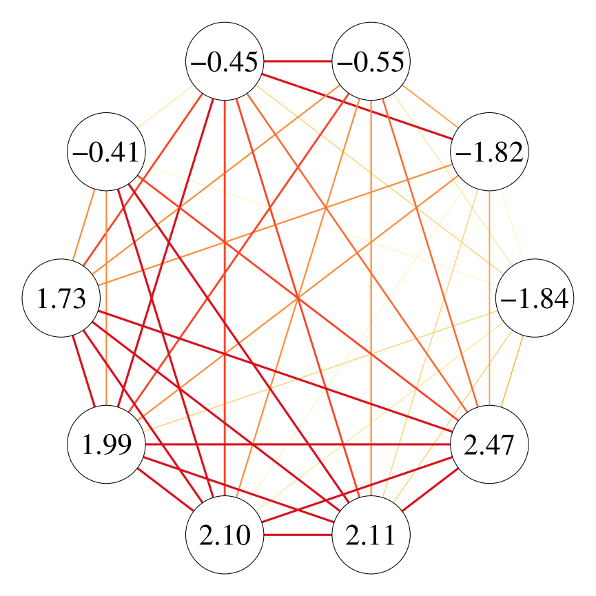
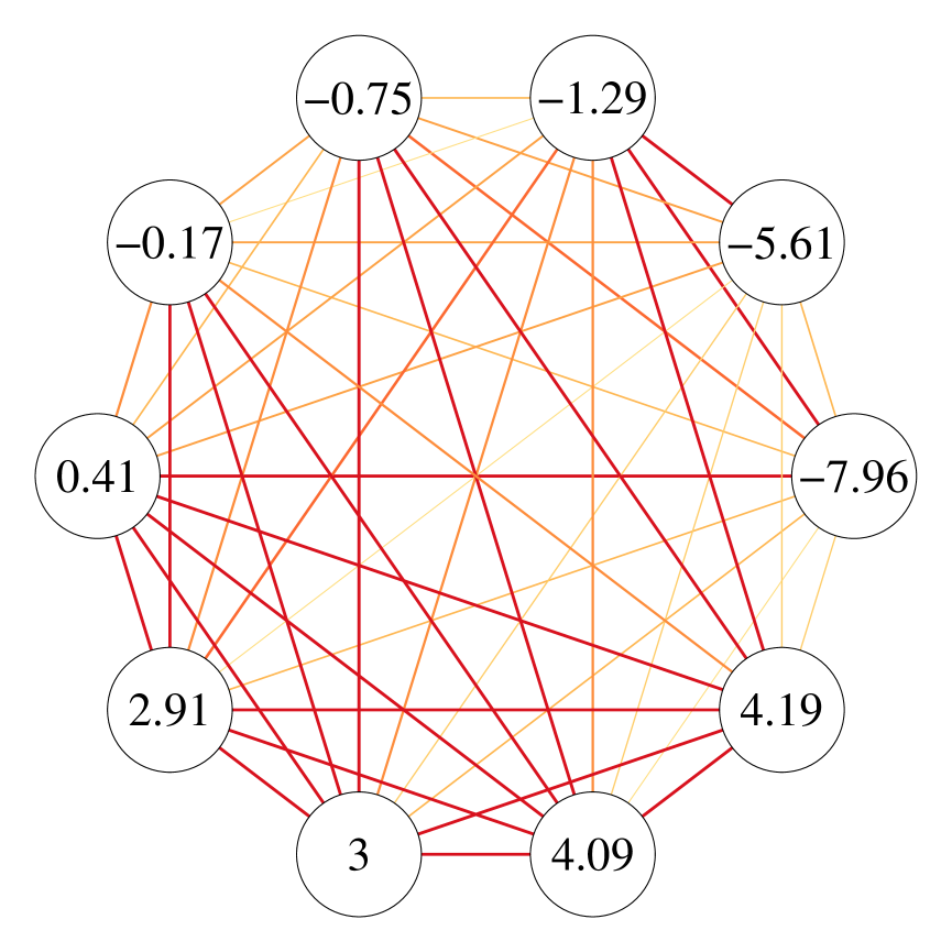
On the other hand, we examine how TWHM can capture dynamic heterogeneity. Towards this, we plot a subgraph of the 10 nodes having the smallest fitted values in Figure 3(b), where edges represent the magnitude of which is a measure of the extent that an edge is preserved across the whole period and hence dynamic heterogeneity. Again, we can see an agreement between the fitted and how likely these nodes will preserve their ties.
To evaluate how TWHM performs when it comes to making prediction, we further carry out the following experiments:
-
(i)
From (1), given the MLE and the network at time , we can estimate the conditional expectation of node ’s degree as
We can then compare the density of the estimated degree sequence with that of the observed degree sequence at time . To provide a comparison, we treat networks in each period as i.i.d. observations and utilize the classical -model to derive the degree sequence estimator for the four periods. The fitted degree distributions are depicted in Figure 4, revealing a close resemblance between the estimated and observed densities. This observation suggests that the TWHM demonstrates strong performance in one-step-ahead prediction.
To further assess the similarity between the estimated degree sequences , , and the true degree sequence , we compute the Kolmogorov-Smirnov (KS) distance and conduct the KS test for . The mean and standard deviation of the KS distances, the p-values of the KS test, and the rejection rate are summarized in Table 5. Notably, at a significance level of 0.05, out of the 40 KS tests, we fail to reject the null hypothesis that and originate from the same distribution in 38 instances, resulting in a rejection rate consistent with the significance level. Conversely, for the degree sequence estimators based on the -model , 8 out of the 40 tests were rejected. These findings indicate that our model exhibits highly promising performance in recovering the degree sequences.
Table 5: The mean and standard deviation of the KS distances, the p-values of KS test, and the rejection rate between the true degree sequence , and the THWM based estimator and the -model based estimator over the 40 networks () in the ant dataset. KS distance KS test p-value Rejection rate vs 0.179(0.058) 0.361(0.267) 0.05 vs 0.192(0.061) 0.298(0.246) 0.20 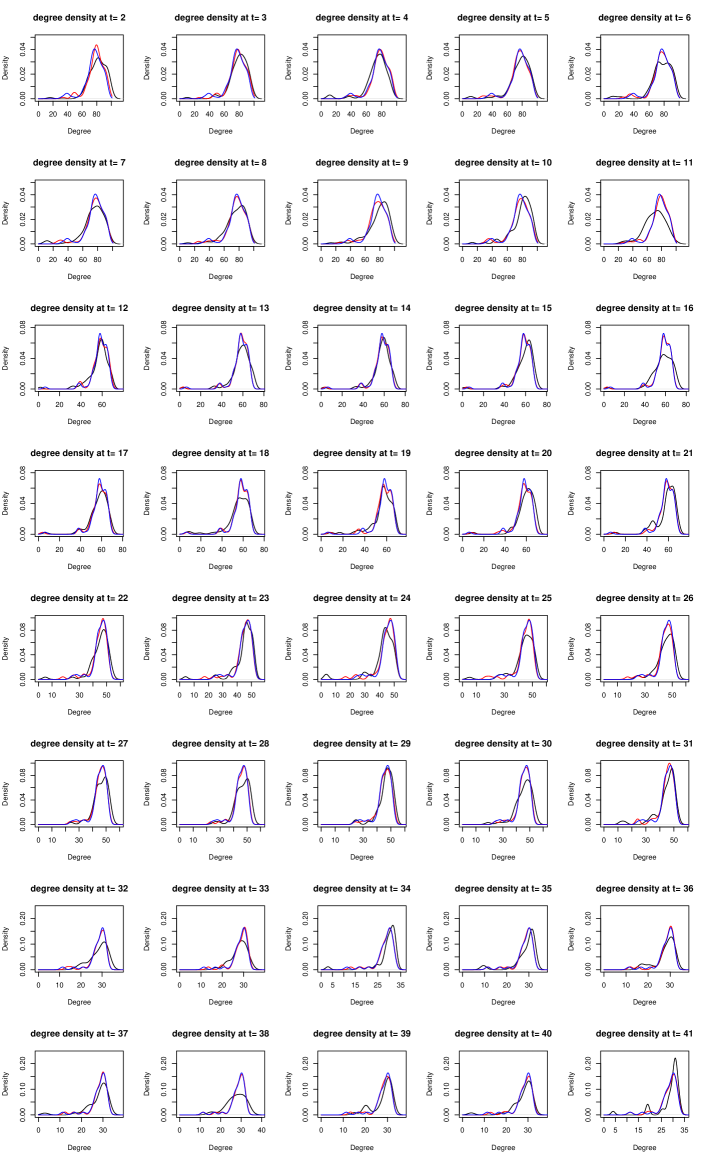
Figure 4: The observed and estimated degree distributions. X-axis: the node degrees; Red curves: the smoothed degree distributions of the estimated degree sequences; Black curves: the smoothed degree distributions of the observed degree sequences. -
(ii)
By incorporating network dynamics, TWHM naturally enables one-step-ahead link prediction via
(5.15) To transform these probabilities into links, we threshold them by setting when and when for some cut-off constants . As an illustration, we first consider simply setting for all for predicting links. We shall denote this approach as TWHM0.5.
As an alternative, owing to the fact that networks may change slowly, for a given parameter , we also consider the following adaptive approach for choosing :
(5.16) It can be shown that the above estimator is equivalent to the prediction rule with cut-off values specified as
This method is denoted as TWHMadaptive. Lastly, as a benchmark, we have also considered a naive approach that simply predicts as .
In this experiment, we set the number of training samples to be or . For a given training sample size and a period with networks, we predict the graph based on the previous networks for . That is, over the four periods in the data, we have predicted 33, 21 and 9 networks, with 5151 edges in each network in the first period, 2628 in the second period, 1485 in the third period, and 595 in the fourth period for our choices of . The parameter employed in TWHMadaptive is selected as follows. For prediction in each period, we choose the value in a sequence of values that produces the highest prediction accuracy in predicting for predicting . For example, in the first period with networks, when , we used to predict for . For each , let be defined as in (5.16). A set of candidate values for were used to compute , and the one that returns the smallest misclassification rate (in predicting ) was used in TWHMadaptive for predicting . The mean of the chosen is when , when , and when . The prediction accuracy of the above-mentioned methods, defined as the percentages of correctly predicted links, are reported in Table 6. We can see that TWHM0.5 and TWHMadaptive both perform better than the naive approach in all the cases. On the other hand, TWHM coupled with adaptive cut-off points can improve the prediction accuracy of TWHM with a cur-off value 0.5 in most periods.
| Period | TWHM0.5 | TWHMadaptive | Naive | |
|---|---|---|---|---|
| 2 | One | 0.773 | 0.800 | 0.749 |
| Two | 0.817 | 0.817 | 0.780 | |
| Three | 0.837 | 0.837 | 0.806 | |
| Four | 0.824 | 0.831 | 0.807 | |
| Overall | 0.811 | 0.822 | 0.784 | |
| 5 | One | 0.789 | 0.807 | 0.759 |
| Two | 0.826 | 0.823 | 0.779 | |
| Three | 0.846 | 0.849 | 0.805 | |
| Four | 0.833 | 0.842 | 0.805 | |
| Overall | 0.822 | 0.829 | 0.786 | |
| 8 | One | 0.795 | 0.800 | 0.759 |
| Two | 0.832 | 0.832 | 0.778 | |
| Three | 0.855 | 0.845 | 0.823 | |
| Four | 0.831 | 0.863 | 0.779 | |
| Overall | 0.825 | 0.831 | 0.782 |
6 Summary and Discussion
We have proposed a novel two-way heterogeneity model that utilizes two sets of parameters to explicitly capture static heterogeneity and dynamic heterogeneity. In a high-dimension setup, we have provided the existence and the rate of convergence of its local MLE, and proposed a novel method of moments estimator as an initial value to find this local MLE. To the best of our knowledge, this is the first model in the network literature that the local MLE is obtained for a non-convex loss function. The theory of our model is established by developing new uniform upper bounds for the deviation of the loss function.
While we have focused on the estimation of the parameters in this paper, how to conduct statistical inference for the local MLE is a natural next step for research. In our setup, we assume that the parameters are time invariant but this need not be the case. A future direction is to allow the static heterogeneity parameter and/or the dynamic heterogeneity parameter to depend on time, giving rise to non-stationary network processes. In case when these parameters change smoothly over time, we may consider estimating the parameters at time by kernel smoothing, that is, by maximizing the following smoothed log-likelihood:
with where is a kernel function and is the bandwidth parameter. As another line of research, note that TWHM is formulated as an AR(1) process. We can extend it by including more time lags. For example, we can extend TWHM to include lag- dependence by writing
where the innovations are independent such that
with parameter denoting node-specific static heterogeneity and denoting lag- dynamic fluctuation. Other future lines of research include adding covariates to model the tendency of nodes making connections [35] and exploring additional structures [3].
References
- Bhattacharjee et al., [2020] Bhattacharjee, M., Banerjee, M., and Michailidis, G. (2020). Change point estimation in a dynamic stochastic block model. Journal of Machine Learning Research, 21(107):1–59.
- Chatterjee et al., [2011] Chatterjee, S., Diaconis, P., and Sly, A. (2011). Random graphs with a given degree sequence. The Annals of Applied Probability, 21(4):1400–1435.
- Chen et al., [2021] Chen, M., Kato, K., and Leng, C. (2021). Analysis of networks via the sparse -model. Journal of the Royal Statistical Society: Series B (Statistical Methodology), 83(5).
- Durante et al., [2016] Durante, D., Dunson, D. B., et al. (2016). Locally adaptive dynamic networks. The Annals of Applied Statistics, 10(4):2203–2232.
- Fu and He, [2022] Fu, D. and He, J. (2022). Dppin: A biological repository of dynamic protein-protein interaction network data. In 2022 IEEE International Conference on Big Data (Big Data), pages 5269–5277. IEEE.
- Gragg and Tapia, [1974] Gragg, W. and Tapia, R. (1974). Optimal error bounds for the newton–kantorovich theorem. SIAM Journal on Numerical Analysis, 11(1):10–13.
- Graham, [2017] Graham, B. S. (2017). An econometric model of network formation with degree heterogeneity. Econometrica, 85(4):1033–1063.
- Han et al., [2020] Han, R., Chen, K., and Tan, C. (2020). Bivariate gamma model. Journal of Multivariate Analysis, 180:104666.
- Han et al., [2023] Han, R., Xu, Y., and Chen, K. (2023). A general pairwise comparison model for extremely sparse networks. Journal of the American Statistical Association, 118(544):2422–2432.
- Hanneke et al., [2010] Hanneke, S., Fu, W., and Xing, E. P. (2010). Discrete temporal models of social networks. Electronic journal of statistics, 4:585–605.
- Hanneke and Xing, [2007] Hanneke, S. and Xing, E. P. (2007). Discrete temporal models of social networks. In Statistical network analysis: models, issues, and new directions: ICML 2006 workshop on statistical network analysis, Pittsburgh, PA, USA, June 29, 2006, Revised Selected Papers, pages 115–125. Springer.
- Hillar et al., [2012] Hillar, C. J., Lin, S., and Wibisono, A. (2012). Inverses of symmetric, diagonally dominant positive matrices and applications. arXiv preprint arXiv:1203.6812.
- Holland and Leinhardt, [1981] Holland, P. W. and Leinhardt, S. (1981). An exponential family of probability distributions for directed graphs. Journal of the American Statistical Association, 76(373):33–50.
- Jiang et al., [2023] Jiang, B., Li, J., and Yao, Q. (2023). Autoregressive networks. Journal of Machine Learning Research, 24(227):1–69.
- Jin, [2015] Jin, J. (2015). Fast community detection by score. The Annals of Statistics, 43(1):57–89.
- Jin et al., [2022] Jin, J., Ke, Z. T., Luo, S., and Wang, M. (2022). Optimal estimation of the number of network communities. Journal of the American Statistical Association, pages 1–16.
- Karrer and Newman, [2011] Karrer, B. and Newman, M. E. (2011). Stochastic blockmodels and community structure in networks. Physical review E, 83(1):016107.
- Karwa et al., [2016] Karwa, V., Slavković, A., et al. (2016). Inference using noisy degrees: Differentially private -model and synthetic graphs. The Annals of Statistics, 44(1):87–112.
- Ke and Jin, [2022] Ke, Z. T. and Jin, J. (2022). The score normalization, especially for highly heterogeneous network and text data. arXiv preprint arXiv:2204.11097.
- Kolaczyk and Csárdi, [2020] Kolaczyk, E. D. and Csárdi, G. (2020). Statistical analysis of network data with R, volume 65. Springer, 2 edition.
- Krivitsky and Handcock, [2014] Krivitsky, P. N. and Handcock, M. S. (2014). A separable model for dynamic networks. Journal of the Royal Statistical Society. Series B, Statistical Methodology, 76(1):29.
- Lin and Bai, [2011] Lin, Z. and Bai, Z. (2011). Probability inequalities. Springer Science & Business Media.
- Matias and Miele, [2017] Matias, C. and Miele, V. (2017). Statistical clustering of temporal networks through a dynamic stochastic block model. Journal of the Royal Statistical Society, B, 79(4):1119–1141.
- Merlevède et al., [2009] Merlevède, F., Peligrad, M., Rio, E., et al. (2009). Bernstein inequality and moderate deviations under strong mixing conditions. In High dimensional probability V: the Luminy volume, pages 273–292. Institute of Mathematical Statistics.
- Mersch et al., [2013] Mersch, D. P., Crespi, A., and Keller, L. (2013). Tracking individuals shows spatial fidelity is a key regulator of ant social organization. Science, 340(6136):1090–1093.
- Minai and Williams, [1993] Minai, A. A. and Williams, R. D. (1993). On the derivatives of the sigmoid. Neural Networks, 6(6):845–853.
- Newman, [2018] Newman, M. (2018). Networks. Oxford university press.
- Pensky, [2019] Pensky, M. (2019). Dynamic network models and graphon estimation. Annals of Statistics, 47(4):2378–2403.
- Sengupta and Chen, [2018] Sengupta, S. and Chen, Y. (2018). A block model for node popularity in networks with community structure. Journal of the Royal Statistical Society: Series B (Statistical Methodology), 80(2):365–386.
- Stein and Leng, [2020] Stein, S. and Leng, C. (2020). A sparse -model with covariates for networks. arXiv preprint arXiv:2010.13604.
- Van der Vaart, [2000] Van der Vaart, A. W. (2000). Asymptotic statistics, volume 3. Cambridge university press.
- Van Der Vaart and Wellner, [1996] Van Der Vaart, A. W. and Wellner, J. A. (1996). Weak convergence. In Weak convergence and empirical processes, pages 16–28. Springer.
- Wainwright, [2019] Wainwright, M. J. (2019). High-dimensional statistics: A non-asymptotic viewpoint, volume 48. Cambridge University Press.
- Wu et al., [2006] Wu, X., Zhu, L., Guo, J., Zhang, D.-Y., and Lin, K. (2006). Prediction of yeast protein–protein interaction network: insights from the gene ontology and annotations. Nucleic acids research, 34(7):2137–2150.
- Yan et al., [2019] Yan, T., Jiang, B., Fienberg, S. E., and Leng, C. (2019). Statistical inference in a directed network model with covariates. Journal of the American Statistical Association, 114(526):857–868.
- Yan et al., [2015] Yan, T., Leng, C., and Zhu, J. (2015). Supplement to “asymptotics in directed exponential random graph models with an increasing bi-degree sequence”. Annals of Statistics.
- Yan et al., [2016] Yan, T., Leng, C., Zhu, J., et al. (2016). Asymptotics in directed exponential random graph models with an increasing bi-degree sequence. Annals of Statistics, 44(1):31–57.
- Yan and Xu, [2012] Yan, T. and Xu, J. (2012). Approximating the inverse of a balanced symmetric matrix with positive elements. arXiv preprint arXiv:1202.1058.
- Yan and Xu, [2013] Yan, T. and Xu, J. (2013). A central limit theorem in the -model for undirected random graphs with a diverging number of vertices. Biometrika, 100(2):519–524.
Appendix A Technical proofs
For brevity, we denote and , and define and similarly based on the true parameter and the MLE .
A.1 Some technical lemmas
Before presenting the proofs for our main results, we first provide some technical lemmas which will be used from time to time in our proofs. Lemmas 4 and 5 below provide further properties about the process .
Lemma 4.
Let We have:
where is the Hadamard product operator, is strictly stationary. Furthermore for any and , we have
is strictly stationary. Furthermore for any and , we have
Proof.
(ii) Let , and (). Similarly, for every , we have
and
For we have,
with
and
Thus,
This proves (ii). ∎
Lemma 5.
Let hold. Under condition (A1) we have,
Proof.
Lemma 6.
Suppose , are independent random variables with
and almost surely. We have, for any constant , there exists a large enough constant such that, with probability greater than ,
Proof.
This is a direct result of Bernstein’s inequality [22]. ∎
A.2 Proof of Proposition 1
A.3 Proof of Lemma 1
Proof.
By Proposition 3 of [14] and Lemma 4, we have that the process is -mixing with exponential decaying rate. Since the mixing property is hereditary, the processes and are also -mixing with exponential decaying rate. From Theorem 1 in [24], we obtain the following concentration inequalities: there exists a positive constant such that,
hold for all . For any positive constant , by setting with a big enough constant , we have, with probability greater than ,
hold for all . ∎
A.4 Proof of Lemma 2
Proof.
Note that for , we have
With and , for all and for , we then have, there exist positive constants such that, for all and where is a small enough constant,
and
Notice that the elements in and are all positive. Denote with and . Then there exists a constant such that,
Here in the last step we have used the fact that for any , where , and the fact that the eigenvalues of is greater or equal to . ∎
A.5 Proof of Lemma 3
Proof.
Define a series of matrices . For , the , , , elements are while other elements are set to be zero. Then all the matrices are independent and
Since are symmetric and centered random matrices, we have . Further, by the definition of , we know that the th, th, th and th elements of are all equal to , while all other elements are zero. Consequently,
Using the Matrix Bernstein inequality (c.f. Theorem 6.17 of [33]), we have
∎
A.6 Proof of Theorem 1
Proof.
Note that for any and , we have
Therefore, is always positive definite. Next we prove that all are positive definite (in probability) by showing that with probability tending to 1,
holds uniformly for all . Note that
We consider first. By setting with some big enough constant in Lemma 3, we have
As , we have with probability greater than ,
| (A.21) |
By Lemma 1 and Lemma 5, we have, uniformly for all and , there exist positive constants , such that, with probability greater than ,
Consequently, from (A.21) we have
Next we derive uniform upper bounds for . When , by Lemma 1, we have, there exist positive constants and such that with probability greater than ,
holds uniformly for all . Similarly, when , by Lemma 1, we have there exist positive constants and such that, with probability greater than ,
holds uniformly for all . Consequently, there exist positive constants and such that, with probability greater than ,
On the other hand, by inequalities (A.4) and (A.4) we have, there exists a positive constant such that
holds uniformly for any where is a small enough constant. Thus, as , for some small enough constant and for some small enough constant , we have, there exist big enough positive constants such that with probability greater than ,
holds uniformly for all . The statements in Theorem 1 can then be concluded. ∎
A.7 Proof of Theorem 2
Proof.
Recall that
and write ; that is,
Define . Note that when is small enough, . By Corollary 4, there exist big enough positive constants such that, with probability greater than ,
holds uniformly for all random variable .
Note that is the minimizer of . By Lemma 2, there exists a constant , such that for all , we have,
Here is a random scalar that may depend on . Consequently, as , with probability greater than , there exists a constant such that
| (A.22) |
Note that the MLE satisfies that and . Therefore we have , and from (A.22) we can conclude that as , with probability tending to 1,
∎
A.8 Proof of Theorem 3
Before presenting the proof, we first introduce a technical lemma.
Lemma 7.
For all s.t. and any positive s.t. , we have:
Here and are the th element of and , respectively.
Proof.
Note that for all , we have and for all , we have . Consequently, for all s.t. , we have,
holds for any positive s.t. . ∎
Next we proceed to the proof of Theorem 3.
Proof of Theorem 3
Proof.
Recall the functions and defined in the proof of Theorem 2. We denote the MLE studied in Theorem 2 as the local minimizer of in . Also, let be the local minimizer of in the ball where
| (A.23) |
for some given constants . Let
| (A.24) |
We then have . Under the condition that for some positive constant , we have when is large enough.
Next we will show that with probability tending to 1, uniformly for all , , the local MLE for , is also the local MLE in a smaller ball where
and . Note that is the minimizer of . Given , the Hessian matrix of evaluated at is a matrix given as:
Following the calculations in Lemma 2, there exists a constant which is independent of , such that, for all , we have
and
Then we have for all ,
Consequently, for any and , there exists a random scalar , s.t.
On the other hand, notice that
By Corollary 4, there exist large enough positive constants and which are independent of such that, with probability greater than ,
holds uniformly for any where . By Lemma 7, as , there exist big enough positive constants and which are independent of such that, with probability greater than ,
holds uniformly for all for any positive s.t. , and . Here in the last step we have used inequality (A.22) and the fact that for all , . Let and , we have, there exists a big enough constant , with probability greater than ,
holds uniformly for all and . Combining the inequalities (A.8) and (A.8), we have, with probability greater than for a large enough constant ,
| (A.28) | ||||
holds uniformly for all , all and .
Combining the inequalities (A.8) and (A.28), we have, with probability greater than ,
holds uniformly for all and all . Notice that the constants , , , , and are all independent of and . This indicates that there exists a big enough constant which is independent of and s.t.
| (A.29) | ||||
Recall that is the local maximizer of in with
Thus far we have proved that: with probability greater than for some large enough constant , uniformly for all , is also within the ball with
| (A.30) |
Now define a series s.t. is defined as in equation (A.24) and . We have:
| (A.31) |
Then, we have for and .
Let where is the smallest integer function. Beginning with , and repeatedly using the result in (A.29) for times, we have, with probability greater than , we can sequentially reduce the upper bound from to:
Here in the last step of above inequality, we have used the fact that when ,
Thus, assuming that , for some positive constant , we have, with probability tending to 1,
∎
A.9 Proof of Theorem 4
For brevity, we denote , with and . We use the interior mapping theorem [6] to establish the existence and uniform consistency of the moment estimator. The interior mapping theorem is presented in Lemma 8.
Lemma 8.
(Interior mapping theorem). Let be a vector function on an open convex subset of and . Assume that s.t.
where N and are positive constants that may depend on and . Then the Newton iterates exists and for all . Moreover, exists, , where denotes the closure of set and .
Proof of Theorem 4.
Proof.
Recall that the is defined as the solution of
For any , define a system of random functions :
As and with a small enough constant , there exist big enough constants such that with probability greater than ,
| (A.32) | |||||
hold for all . For brevity, the proof of inequalities in (A.32) is provided independently in Section A.10. Let and . Here the notation denotes the interior of a given set . We then have:
Note that , , we have
Consequently, by Lemma 8, we have that, with probability tending to 1,
| (A.33) |
Next, we derive the error bound of based on (A.33). For , define a system of random functions :
As and with a small enough constant , there exist big enough constants such that with probability greater than ,
| (A.34) | |||
hold for all . For brevity, the proof of inequalities in (A.34) is provided independently in Section A.11. Let and . We then have:
Note that , , we have
Consequently, by Lemma 8, we have that, with probability tending to 1,
Combining with (A.33), the theorem is proved. ∎
A.10 Proof of (A.32)
Proof.
Note that is a balanced symmetric matrix s.t.
for and . Following [38], we construct a matrix to approximate the inverse of . Specifically, for any , we set
Note that
we have
By Theorem 1 in [38], with and , there exists a big enough constant , we have that
where . Then, there exists a big enough constant ,
By Lemma 1 and Lemma 6, there exist big positive constants such that, with probability greater than ,
| (A.35) | ||||
Then, for any with , we have that
| (A.36) |
There exists a big enough constant , we have, for every ,
where with a series of constants . Combining the inequalities (A.35), (A.36) and (A.10), we finish the proof of (A.32). ∎
A.11 Proof of (A.34)
Proof.
For brevity, is denoted by . Moreover, as all the conclusions hold uniformly for all , the argument “uniformly for all ” are also omitted in what follows.
Note that is a balanced symmetric matrix s.t.
for and . Following [38], we construct a matrix to approximate the inverse of . Specifically, for all , we set
Note that there exists a big enough constant s.t., for any ,
we have
| (A.38) |
By Theorem 1 in [38], with and , there exists big enough constant , we have that
where . Then we have that
Moreover, we have that
By Lemma 1 and Lemma 6, there exist big positive constants s.t., with probability greater than ,
Moreover, we have
where with a series of constants . Then, by equation (A.33), there exists a big enough constant , we have, with probability tending to 1,
We can conclude that, with probability tending to 1,
hold uniformly for any at the same time. Consequently, we have
There exists an big enough constant , we have, for every ,
| (A.41) | ||||
where with a series of constants . Combining the inequalities (A.11), (A.11) and (A.41), we finish the proof of (A.34). ∎
A.12 Proof of Corollary 1
Proof.
A.13 Proof of Corollary 2
Proof.
The first inequality can be proved using the results in Corollary 1, along with analogous reasoning employed in the proof of Theorem 1. Replace equations (A.23) and (A.24) by
Similar to the proof of Theorem 3, let and . We can assert the existence of a sufficiently large constant such that with probability greater than ,
holds uniformly for all and . Following similar steps, we can ascertain that as with , with probability converging to one it holds that
∎
A.14 Proof of Corollary 3
A.15 Proof of the Theorem 5
Proof.
To simplify the notations, in what follows we shall denote as instead. Let for some big enough constant , where is the smallest integer function. By the Taylor expansion with Lagrange remainder we have, for any , there exists a dependent on s.t.,
We first consider . By Lemma 6, there exist big enough constants such that, uniformly for all and all , we have, with probability greater than ,
Consequently, with probability greater than we have:
holds uniformly for all . Note that for any s.t. for some constant , we have
| (A.42) |
Here in last step we have used . With the fact that holds for any , we have, with probability greater than ,
Next we derive an upper bound for . Define a series of random matrices with the -th elements of given as
Further for any , define a random matrix as:
Also we define a series of vectors, with -th element of given as:
For any , by denoting as:
we have:
We remark that by formulating the confounding terms in via , we have established in (A.15) an upper bound that depends on the parameters in and the random matrices separately. Using the fact that , we have
Consequently, there exists a big enough constant such that, for all , we have
Here the last step follows from (A.42). With similar arguments as in the proof of the matrix Bernstein inequality (c.f. Lemma 3), we can show that uniformly for all , there exist big enough constants and , such that with probability greater than ,
| (A.45) |
For brevity, the proof of inequality (A.45) is provided independently in Section (A.16). Consequently, combining (A.15), (A.15) and (A.45) and , we conclude that with probability greater than ,
uniformly for all . Finally, we derive an upper bound for . By condition (L-A1), when is chosen to be big enough, there exists a big enough constant , such that, uniformly for all and , we have
Here the last step will hold if we choose to be large enough such that . When , and are chosen to be large enough, this bound will be dominated by the upper bounds for and .
Combining the upper bound on and , we conclude that, for any given , there exist large enough constants , which are independent of such that for any where at the same time with probability greater than ,
∎
A.16 Proof of inequality (A.45)
Proof.
For any and , let be defined by keeping the th element of all the in unchanged, and setting all other elements to be zero. Then the random matrices , are independent, and
For any , we can write it as
with , . Then for any and , we have,
On the other hand,
Using the general Matrix Bernstein inequality (c.f. Theorem 6.17 and equation (6.43) of [33]), we have,
Consequently, there exist big enough constants and s.t. by choosing
we have, with probability greater than ,
holds for all where is big enough constant. ∎
A.17 Proof of Theorem 6
Proof.
For any vector , we define . With similar arguments as in the proof of Theorem 5, we have that there exists a such that
where for some large enough constant . First consider . There exist big enough constants , such that, uniformly for all , and all , we have, with probability greater than ,
Then, from inequality (A.42) we have, there exist big enough constants and , such that with probability greater than ,
holds uniformly for and .
Next we derive an upper bound for . With the fact that and
by Lemma 6 we have, there exist big enough constants such that with probability greater than ,
Consequently, there exists a big enough constant such that, uniformly for all and , we have, with probability greater than ,
Here in the above inequalities we have used that fact that , and the last step follows from the inequality (A.42).
Finally, we derive an upper bound for . By condition (L-A1), by choosing with to be a large enough constant, there exists a big enough constant such that, uniformly for all , and , we have
Here the last step will hold if we choose to be large enough such that . When , and are chosen to be large enough, this bound will be dominated by the upper bounds for and .
Consequently, by choosing with to be a large enough constant, we conclude that, for any given , there exist large enough constants such that uniform for any and , with probability greater than ,
∎
Appendix B Additional numerical results
B.1 Informal justification of the use of TWHM in analyzing the insecta-ant-colony4 dataset
To motivate the use of the proposed TWHM for the analysis of the insecta-ant-colony4 dataset, we plot the autocorrelation function (ACF) and the partial autocorrelation function (PACF) of the degree sequences of two ants. These ants are selected based on their respective highest and lowest values at time according to
Upon examining Figure 5, it becomes evident that both degree sequences exhibit patterns reminiscent of a first-order autoregressive model with long memory. This observation serves as a strong motivation for employing the TWHM methodology.
B.2 Community detection under stochastic block structures
We conduct additional numerical studies to assess the efficacy of community detection using the estimated -parameters. To implement stochastic block structures within the TWHM framework, we partitioned the nodes into communities of equal size, ensuring that the parameters for all nodes within the same community were identical. Furthermore, we explored scenarios where the networks were independently generated from a Stochastic Block Model (SBM). Specifically, we have considered the following settings:
-
Setting 1: The networks are generated under TWHM with for all nodes in communities and respectively.
-
Setting 2: The networks are generated under TWHM with for all nodes in communities and respectively.
-
Setting 3: The networks are independently generated under SBM, with the probability matrix among different communities specified as
-
Setting 4: The networks are independently generated under SBM, with the probability matrix among different communities given by
-
Setting 5: The networks are independently generated under SBM, with the probability matrix among different communities given by
Networks in Settings 1-2 are generated with autoregressive dependence using our TWHM model, while networks in Setting 3 are independent samples following the classical SBM structure. In Settings 4-5, networks are also generated with SBM structures, but the probability formation matrices are not full-rank.
Once the -parameters are estimated, we apply k-means clustering to these parameters to cluster the nodes, denoting this method as ”TWHM-Cluster”. For comparison, we apply spectral clustering, widely used for SBM, on the averaged networks, denoting this method as ”SBM-Spectral”. All experiments are repeated 100 times, and the clustering accuracy is reported in Table 7 below.
From Table 7, we observe that community detection using the -parameters performs significantly better under Settings 1 and 2, where data were generated from our TWHM model. This improvement is attributed to the fact that parameter estimation has considered the autoregressive structure of the networks.
When networks were independently generated from SBM under Setting 3, the performance of TWHM-Cluster is comparable to that of SBM-Cluster. However, when the probability matrix of SBM is not full-rank (Settings 4 and 5), the TWHM model still demonstrates promising performance, while classical spectral clustering can be much less satisfactory.
| TWHM-Cluster | SBM-Spectral | ||
|---|---|---|---|
| Setting 1 | (3,2,300) | 68.6% | 37.1% |
| (3,10,300) | 95.1% | 37.0% | |
| (3,50,300) | 99.5% | 38.7% | |
| Setting 2 | (3,2,300) | 92.2% | 39.7% |
| (3,10,300) | 95.6% | 48.6% | |
| (3,50,300) | 100.0% | 63.0% | |
| Setting 3 | (3,10,300) | 92.1% | 99.8% |
| (3,30,300) | 99.4% | 100.0% | |
| (3,50,300) | 99.3% | 100.0% | |
| Setting 4 | (3,10,500) | 97.0% | 37.1% |
| (3,30,500) | 93.9% | 37.0% | |
| (3,50,500) | 100% | 37.5% | |
| Setting 5 | (3,10,500) | 80.0% | 71.2% |
| (3,30,500) | 80.2% | 70.7% | |
| (3,50,500) | 83.8% | 72.8% |
B.3 Dynamic protein-protein interaction networks
In this section, we applied the proposed TWHM to 12 dynamic protein-protein interaction networks (PPIN) of yeast cells examined in [5]. Each dynamic network comprises 36 network observations. The objective of investigating protein-protein interactions is to glean valuable insights into the cellular function and machinery of a proteome [34]. To provide an overview of these datasets, we present selected statistics in Table 8.
| Dataset | # of Nodes | Mean degree | Density |
|---|---|---|---|
| DPPIN-Uetz | 922 | 4.68 | 0.22% |
| DPPIN-Ito | 2856 | 6.05 | 0.07% |
| DPPIN-Ho | 1548 | 54.55 | 0.13% |
| DPPIN-Gavin | 2541 | 110.22 | 0.08% |
| DPPIN-Krogan (LCMS) | 2211 | 77.01 | 0.09% |
| DPPIN-Krogan (MALDI) | 2099 | 74.60 | 0.10% |
| DPPIN-Yu | 1163 | 6.19 | 0.17% |
| DPPIN-Breitkreutz | 869 | 90.33 | 0.23% |
| DPPIN-Babu | 5003 | 44.56 | 0.04% |
| DPPIN-Lambert | 697 | 19.09 | 0.29% |
| DPPIN-Tarassov | 1053 | 9.17 | 0.19% |
| DPPIN-Hazbun | 143 | 27.40 | 1.40% |
We have employed our method for linkage prediction on these PPINs. Similar to the main paper, we utilized TWHM with either a fixed cutoff point of (TWHM0.5) or the adaptive rule (TWHMadaptive). For comparison, we used a naive estimator to predict (Naive). Our training time slot size was set to , and the results are presented in Table 9 below. As evident from the table, our approach shows significant promise for accurate link prediction.
| Dataset | TWHM0.5 | TWHMadaptive | Naive | |
|---|---|---|---|---|
| DPPIN-Uetz | 55 | 55 | 88 | |
| DPPIN-Ito | 28 | 29 | 50 | |
| DPPIN-Ho | 108 | 111 | 194 | |
| DPPIN-Gavin | 139 | 142 | 250 | |
| DPPIN-Krogan(LCMS) | 133 | 141 | 222 | |
| DPPIN-Krogan(MALDI) | 124 | 127 | 215 | |
| DPPIN-Yu | 54 | 55 | 86 | |
| DPPIN-Breitkreutz | 297 | 305 | 493 | |
| DPPIN-Babu | 27 | 28 | 45 | |
| DPPIN-Lambert | 293 | 298 | 489 | |
| DPPIN-Tarassov | 72 | 75 | 133 | |
| DPPIN-Hazbun | 759 | 772 | 1198 |