A Two-Stage Training Framework for Joint Speech Compression and Enhancement
Abstract
This paper considers the joint compression and enhancement problem for speech signal in the presence of noise. Recently, the SoundStream codec, which relies on end-to-end joint training of an encoder-decoder pair and a residual vector quantizer by a combination of adversarial and reconstruction losses, has shown very promising performance, especially in subjective perception quality. In this work, we provide a theoretical result to show that, to simultaneously achieve low distortion and high perception in the presence of noise, there exist an optimal two-stage optimization procedure for the joint compression and enhancement problem. This procedure firstly optimizes an encoder-decoder pair using only distortion loss and then fixes the encoder to optimize a perceptual decoder using perception loss. Based on this result, we construct a two-stage training framework for joint compression and enhancement of noisy speech signal. Unlike existing training methods which are heuristic, the proposed two-stage training method has a theoretical foundation. Finally, experimental results for various noise and bit-rate conditions are provided. The results demonstrate that a codec trained by the proposed framework can outperform SoundStream and other representative codecs in terms of both objective and subjective evaluation metrics. Code is available at https://github.com/jscscloris/SEStream.
Index Terms:
Speech compression, speech enhancement, noise reduction, codec, neural networksI Introduction
Audio codec is a fundamental tool for audio transmission. Recently, benefited from the powerful deep learning techniques, neural networks based audio codecs have made much progress and shown considerable improvement over traditional digital signal processing based codecs. Generally, neural networks based codecs can be divided into two categories. The first is based on generative models [6, 26, 28, 27, 29, 30], which aims to generate high-fidelity speech from compressed representation. The second is based on end-to-end neural network models, which learns an encoder-decoder pair in an end-to-end manner [31, 32, 8, 33, 55, 56]. Generative models, such as WaveNet [22], WaveRNN [24], and WaveGRU [6], are typically combined with traditional codec algorithms. Given compressed representation from traditional codecs, these models have shown impressive performance in generating high perception quality audio [6, 26, 28, 27, 29, 30]. End-to-end models [31, 32, 8, 33] aim to encode audio into a bit stream at a target bit-rate, and then recover the source audio from the bit stream in an end-to-end way using methods like variational autoencoder (VAE) [34, 9]. While these methods have achieved remarkable performance, how to construct an optimal training framework for end-to-end codec model in the presence of noise is still an open question.
High perception quality is a main goal of audio codecs, which measures the degree to which the decoded audio sounds like natural clean audio from human subjective judgement. Taking perception quality into consideration, audio codecs typically aim to encode audio into as few bits as possible and, at meantime, reconstruct audio with less distortion and better perceptual quality as possible. Intuitively, the quality of the reconstructed audio depends on the bit-rate. The lower the bit-rate, the worse the quality of the reconstructed audio. Recently, it has been shown both theoretically and empirically that, at a given bit-rate, there is a tradeoff between distortion and perception [11, 23, 13, 14]. That is, to achieve high perception quality, an elevation of the lowest achievable distortion is necessary. Accordingly, there is three way tradeoff between bit-rate, distortion, and perceptual quality. To achieve high perception quality, the recent work SoundStream [8] employs a combination of adversarial and reconstruction losses to train an end-to-end encoder-decoder model, in which a residual vector quantizer is jointly trained for bit-rate scalable codec. SoundStream has shown remarkable performance in perception quality especially in low bit-rate case.
In many practical applications, audio codecs inevitably suffer from background noise from the environment. In the presence of noise, a straightforward approach is to use a cascade of a denoising model and a codec, which firstly employs a denoising model to suppress the noise in the noisy signal and, then, processes the denoised signal by the codec. In theory, this combination approach using two cascaded models is optimal in compressing noisy signal [62, 63]. However, in practice, using two models for denoising and compression respectively is more complex and would incur larger latency compared with a single model for joint denoising and compression. Recently, some works have studied the joint speech enhancement and compression problem using neural models. For example, based on VQ-VAE autoencoder with WaveRNN decoder, the work [52] proposes a compressor-enhancer encoder for audio codec in noisy conditions. The work [4] proposes an end-to-end neural speech codec with low latency, namely TFNet, which is jointly optimized with speech enhancement and packet loss concealment. In [5], the separation of speech signal from background noise in compressed domain of a neural audio codec has been considered. Moreover, SoundStream [8] shows that compression and enhancement can be jointly considered, which achieves controllable noise reduction through a FiLM layer [10].
Though straightforward training of an end-to-end codec model using noisy speech data can naturally make the learned model robust to noise, how to construct an optimal end-to-end training framework for joint speech compression and enhancement in the presence of noise is still an open question. Existing methods typically use a heuristic combination of distortion and adversarial losses to achieve high perception quality, which lacks theoretical foundation.
This paper provides a theoretical analysis on the joint speech compression and enhancement problem, which considers a lossy compression model under both distortion and perception quality constraints. The analysis sheds some light on how to construct an optimal training framework for speech compression in the presence of noise. Based on the result, we develop a two-stage training framework and evaluate it in various bit-rate and noise conditions in comparison with existing methods.
The main contributions of this work are as follows.
-
•
We provide a theory for optimally training of joint speech compression and enhancement in the presence of noise. The theoretical result reveals that to simultaneously achieve low distortion and high perception quality for joint compression and enhancement in the presence of noise, an optimal optimization procedure is given by a two-stage optimization that, firstly, optimizes an encoder-decoder pair using only distortion loss and, then, fixes the obtained encoder to optimize a perceptual decoder using perception loss.
-
•
Based on the theoretical result, we construct a two-stage training framework for joint compression and enhancement of noisy speech signal. To achieve satisfactory performance on speech signal, multi-scale time-frequency spectrum based reconstruction loss and multi-scale adversarial loss are employed.
-
•
The proposed method is evaluated in comparison with state-of-the-art speech codecs, including SoundStream, Lyra, EVS, and OPUS. Experimental results under various noise and bit-rate conditions show that the proposed two-stage method can achieve better performance in terms of both objective and subjective evaluation metrics than state-of-the-arts.
II Related work
II-A Audio Codecs
Audio codec is a fundamental technique in audio communication, which aims to compress audio signal at a given bit-rate with distortion as less as possible. Classic audio codecs include USAC[1], EVS[3] and OPUS[2]. USAC (Unified Speech and Audio Coding) is a low-delay, high-quality audio coding standard developed by MPEG. OPUS is an open-source audio codec with sampling rates ranging from 6 kbps to 510 kbps. It supports a wide range of audio applications from video conferencing to streaming media services. The performance of OPUS is excellent in high bit-rate compression. EVS (Enhanced Voice Services) is the latest codec developed by 3GPP standardization organization for mobile networks. It supports target bit-rates ranging from 5.9 kbps to 128 kbps and performs better than OPUS at medium and low target bit-rate.
Generative model has become a popular tool for audio reconstruction tasks due to its ability to generate high-quality audios. Wavenet[22, 57] is an auto-regressive sequence generation model, which can directly generate high-quality speech waveforms from input signal. Based on it, a series of generative models such as WaveRNN[24], WaveGAN[49], and Parallel WaveGAN[50] have been developed as vocoder for text-to-speech, which further improve the speed of processing and quality of the reconstructed audio. Lyra[6] utilizes an auto-regressive WaveGRU model as the decoder of the codec. It can achieve excellent performance at a low target bit-rate of 3 kbps. Another type of MelGAN-based generative models mainly focuses on improved discriminators for audio signal, which can improve perceptual quality by a large margin. For example, MelGAN [19] proposes to use multi-scale discriminators to achieve better perception quality. Furthermore, HIFI-GAN [12] designs a multi-period discriminator and proposes a multi-receptive field fusion method. Based on HIFI-GAN, Fre-GAN [51] uses DWT to retain high-frequency information and uses RCG to capture information of different frequency bands. These methods have shown effectiveness in improving naturalness of generated speech.
Recently, end-to-end neural audio codecs have shown promising performance. The work [31] proposes a neural network architecture based on VQ-VAE and WaveNet decoder. It can generate high-quality audio at a very low bit-rate of 1.6 kbps. The work [32] introduces a speaker encoder and speaker VQ codebook into the VQ-VAE architecture to generalize to unseen speakers or content. SoundStream [8] proposes a bit-rate scalable codec with VQ-VAE-2 [9], which can support scalable bit-rates from 3 kbps to 18 kbps with a single model by simply controlling the number of cascaded VQs during inference.
II-B Speech Enhancement
Speech enhancement, also known as noise reduction, aims to remove the background noise of observed noisy speech. It is widely used as a front-end processing technology in speech recognition, hearing aids, and telephone communication. Generally speaking, speech enhancement methods can be divided into two categories, the traditional statistical model based methods [59, 60, 61], and the recent DNN-based methods [35, 37, 36, 38, 7, 44, 45, 46, 47, 48, 53, 54, 58, 39, 40, 43, 41, 42]. Traditional methods, such as the spectral subtraction method, the statistical model based method, and the subspace based method, perform well on the suppression of stationary noise. However, these methods often perform poorly on non-stationary noise.
Benefited from the powerful deep learning technique, DNN-based methods can achieve significantly better performance than the traditional statistical model based methods [37, 36, 38, 7, 44, 45]. However, the most popular speech codecs, such as EVS and OPUS, do not consider speech denoising or use cascaded denoising module. OPUS applies discontinuous transmission (DTX) to reduce the impact of noise by reducing the bit-rate of silent frames or noisy frames and applies noise shaping filters to reduce noise. EVS uses DTX and Comfort Noise Generation (CNG) to handle noisy speech. It employs Voice Activity Detection (VAD) to detect silent segments or background noise, encodes the noise with dedicated cores and finally compensates the distortion in speech with CNG. Another popular speech codec Lyra still applies an additional module TasNet [7] for noise suppression before the encoding the signal. To improve this cascaded structure, SoundStream proposes that compression and enhancement can be jointly performed by the single model without increasing the overall delay. It uses Feature-wise Linear Modulation (FiLM) [10] to achieve controllable denoising. The FiLM layer performs a simple feature-wise affine transformation on the features of the intermediate layer of the neural network and dynamically activates and deactivates the denoising with an additional conditioning signal.
II-C The Rate-Distortion-Perception Tradeoff
In speech codec, the objective is to achieve lower distortion and higher perceptual quality at a given bit-rate. Recent studies show that distortion and perception quality are at odd with each other. More specifically, minimizing distortion only would not necessarily lead to good perception quality. Imposing perfect perception quality constraint would lead to increase of the lowest achievable distortion [11, 23]. That is high perception quality can only be achieved at the cost of increased distortion. In the field of audio processing, the commonly used spectral reconstruction loss is also a kind of distortion loss. Therefore, only considering the spectral distortion of the reconstruction is not enough for achieving high perception quality. Mathematically, perceptual quality can be expressed as the deviation between the distribution of the decoded signal and that of the source signal , as [11]
| (1) |
where is a divergence measures the deviation between two distributions, such as the KL divergence or Wasserstein distance, which satisfies if and only if . When , and have the same distribution as . In this case, the reconstruction has perfect perception quality.
As generative adversarial training is effective in aligning distributions, adversarial loss is widely used in learning deep neural networks based codecs to minimize the deviation between the distributions of the decoded output and the source , i.e., . It has been shown that, such adversarial training can significantly improve the naturalness of the generated audio. However, using only adversarial loss can result in excessive increase of the reconstruction distortion, e.g, though the decoded output can have good perception quality but with large distortion from the input signal. Therefore, adversarial loss is usually used in combination with distortion loss such as spectral reconstruction loss, with a balance between these two losses to achieve a trade-off between distortion and perception [19, 12, 8]
Recently, the works [13, 14] have studied the training framework for perceptual lossy compression under perception constraint. A method for flexibly controllable perception-distortion trade-off has been proposed in [14]. For audio codec, there also exist a perception-distortion trade-off problem, as empirically shown in [8]. As the work [13] considers the lossy compression problem in the absence of noise, the results do not apply to audio codec in processing noisy speech signal. Speech noise is inevitable in many real-world applications. In this work, we extend the work [13] to consider the joint compression and enhancement of noisy speech signal.
III Theory and Methodology
III-A Analysis on Joint Compression and Enhancement
We first review existing results on the compression problem in the absence of noise and, then, present extended results on the joint compression and enhancement problem in the presence of noise.
Suppose that is a deterministic discrete source to be compressed. In the speech compression task without considering noise, an encoder encodes the source signal into a sequential compressed representation at a given bit-rate , and a decoder decodes the compressed representation to obtain , which can be written as
At a given bit-rate , the rate-distortion-perception (R-D-P) function for perceptual lossy compression, which additionally takes perception quality constraint into consideration in the Shannon’s rate-distortion function, can be expressed as
| (2) | ||||
where stands for the distortion constraint, stands for the perception quality constraint based on the divergence between and , and is a distortion measure function. For the R-D-P problem (2), the following result has been derived in [13].
Theorem 1 [13]: Suppose that is a deterministic discrete source, and the distortion function measures the squared error. Let be an optimal encoder-decoder pair to problem (2) in the case without any constraint on perception, i.e. in (2), then is also an optimal encoder in the case perfect perception constraint i.e. in (2). Furthermore, denote , there holds the following equations:
| (3) | |||
This result implies that any optimal encoder achieving the minimum mean squared error (MSE) in the case without perception constraint is also an optimal encoder in the case with perfect perception constraint. That is any optimal encoder to is also an optimal encoder to . Next we consider the condition in the presence of noise and provide extended result.
Theorem 2: Let be a deterministic discrete source, and be a noisy observation from as , where is noise. Suppose that is independent with and the distortion function measures the squared error, then, any optimal encoder under the condition without any perception constraint, i.e., in (2), is also an optimal encoder under the condition with perfect perception constraint, i.e., in (2).
Proof: The minimum MSE codec process in the presence of noise can be expressed as
Denote the output of the optimal noise reduction by
Under the condition that measures the squared error, the optimal process for joint compression and noise reduction can be written as
where is the minimum MSE codec output from . Given , and are independent of each other since the data process is a Markov chain. Then for the distortion term, we have
| (4) |
Under the condition that the noise is independent of the clean source , we have and then it follows from (4) that
| (5) | ||||
It implies that the an end-to-end optimization from to is equivalent to the two-stage optimization process which firstly conduct noise reduction to obtain and then compresses by the codec. Thus, we can conclude that under the assumption of independent noise, Theorem 2 holds, and the denoised minimum MSE encoder is still an optimal encoder under the condition with perfect perception constraint.
In speech codec model training, spectral reconstruction loss is usually used rather than the MSE loss for distortion measurement. Particularly, the multi-scale spectral reconstruction loss has been widely used in high-fidelity audio synthesis and has show superior performance. The multi-scale spectral reconstruction loss is typically defined as [25]
| (6) | ||||
where denotes the -th frame of the time-frequency spectrum (or Mel-spectrogram) of the input signal with a window length equals to . denotes the spectrogram of the reconstructed signal . is a balance parameter which is typically chosen to be [8]. The loss (6) computes the distortion of the spectrum and the distortion of the log-scale spectrum for multiple scales in the spectral domain. Though Theorem 2 is only derived for the case of the MSE loss, it still sheds some light on the cases with other distortion losses such as (6).
The above analysis considers the MSE loss. For speech signal processing, the multi-scale spectral reconstruction loss (6), which consists of distance on the spectrogram slice and distance on the log of the spectrogram slice, has shown superiority and hence be widely used in practice. Next, we provide further analysis for the multi-scale spectral reconstruction loss to show that Theorem 1 in the MSE distortion case can be extended to norm case and logarithmic MSE case.
Let be the decoding output which minimizes a generalized distortion such as the distance with respect to the spectrogram slice or the distance with respect to the log of the spectrogram slice. Meanwhile, let denote the output with perfect perception constraint. According to the principle of Markov chain, and are independent of each other.
For the case of the loss, the distortion is distance with respect to the spectrogram slice as
| (7) | ||||
For the case of the log MSE loss, the distortion is distance with respect to the log of the spectrogram slice as
| (8) | ||||
Under the perfect perceptual constraint, i.e. , we can derive perfect perceptual quality by . In the final expansion of (8), the angle between the two inner products of the third term is 180°, therefore the third term is negative. Thus it follows from (8) that
| (9) | ||||
In (7) and (9), the first term is the distortion between the source and the minimum distortion decoding output, and the second term is the distortion caused by mapping to with the same distribution as the source. According to Theorem 1, optimizing the encoder in the case of results in minimizing the upper bound of the minimum distortion in the case of . Therefore, for the multi-scale spectral reconstruction loss in (6), which is composed of loss and log MSE, the minimum distortion encoder in the case without any perception constraint (i.e. ), can also be used as an approximately optimal encoder in the case with perfect perception constraint (i.e. ).
III-B Proposed Training Framework for Joint Speech Compression and Enhancement
From the above analysis, in this subsection we propose a two-stage training framework for joint speech compression and enhancement based on generative adversarial training, in which a generator consists of an encoder-decoder pair is the codec model to be learned, as shown in Fig. 1.
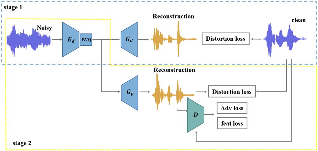
The generator includes an encoder, a residual vector quantizer and a decoder. It firstly compresses the source signal into compressed representation, then encodes it with a series of cascaded vector quantizers, and finally reconstructs the source signal with the decoder. The encoder consists of a one-dimensional convolution layer and four encoding modules with stride . Each encoding module consists of three residual units and a down-sampling layer. Finally, a one-dimensional convolution layer is used to obtain features with a dimension of 256. In order to enable real-time inference, all convolutions are causal. The decoder adopts a similar up-sampling structure. The residual vector quantizer consists of cascaded vector quantizers as in [8]. The target bit-rate of the codec can be calculated by , where is the size of codebook and is the number of frames per second. We also use quantizer dropout in training to enable bit-rate scalability as in SoundStream [8].
The discriminator is employed for adversarial training to improve the perception quality of reconstructed audio. It consists of a waveform-based discriminator and an STFT-based discriminator. The waveform-based discriminator inputs the original audio waveform, two times down-sampled waveform and four times down-sampled waveform, respectively, extracting waveform features from different scales. The STFT-based discriminator first performs STFT transform on the waveform, and then performs 2-D convolution on the time-frequency spectrum to extract features.
Based on the Theorem 2, we propose a two-stage training approach for end-to-end speech codec learning to achieve joint compression and enhancement, as shown in Fig. 1. The generator is an encoder-decoder pair composed of an encoder , a quantizer and a decoder . From Theorem 2, an optimal training procedure contains two steps:
i) In the first step, the encoder-decoder pair is trained using distortion loss only, e.g., with the multi-scale spectral reconstruction loss as (6), without using any discriminator.
ii) In the second step, the encoder and the vector quantizer learned in the first stage are frozen, and a new decoder is trained by a combination of distortion loss and adversarial loss.
Though in theory the perceptual decoder can be trained only by adversarial loss, intensive experiments show that a combination of distortion loss and adversarial loss can yield better performance. This is because it is difficult to train a decoder to reconstruct the signal from compressed representation only using adversarial loss. In the second stage, the overall loss for the generator consists of three components
| (10) | ||||
where is the multi-scale spectral reconstruction loss (6). Similar to [8], we consider 4 individual discriminators, for , with the index denoting the STFT-based discriminator and denoting waveform-based discriminator for different resolutions. With these discriminators, is an adversarial loss for the generator as
| (11) |
where is the number of logits at the output of the -th discriminator along the time dimension.
is a feature loss computed based on the discrepancy between the internal layer outputs of the discriminators, i.e., the difference on the features of the discriminators, as
| (12) |
where is the number of discriminators, is the number of internal layers of each discriminator. is the output of -th layer of the -th discriminator. The discriminator is trained by a loss as
| (13) | ||||
In the first stage of training, we aim to minimize the distortion by the multi-scale spectral reconstruction loss and achieve maximal noise suppression in the encoder . In the second stage of training, we use generative adversarial training so that the decoder can generate high perception quality audio. In order to avoid excessive distortion elevation in adversarial training of the perceptual decoder, the distortion loss is also used in combination with the adversarial loss to achieve a satisfactory performance in practice.
IV Experiments
IV-A Datasets and Training
We train our model on various noise conditions using clean and noisy speech datasets. For clean speech, we use the train-clean-100 and train-clean-360 of LibriTTS [15] as clean speech dataset, which has a sampling rate of 24 kHz. LibriTTS corpus is constructed from audiobooks and includes the speech data from 2456 different speakers. In data pre-processing, we filter out the samples which are resampled from 16 kHz to 24 kHz in the LibriTTS, resulting in 147k clean samples. We generate noisy speech by mixing natural noise with clean speech at a sampling rate of 24 kHz. We use Freesound [16] as natural environmental noise. Freesound contains music, mechanical noise, natural atmosphere and many other kinds of audio. We choose unlicensed audio without human voice as noise data. Different noise segments are inserted into clean speech every three seconds. The signal-to-noise ratio (SNR) is uniformly distributed between 0 dB and 15 dB. Finally, we train our model on 147k clean speech and 33k noisy speech.
To enable bit-rate scalability without retraining the model, Residual Vector Quantizer[20] and Quantizer Dropout[8] are used in the training of all our model. We cascade 24 vector quantizers, each with a codebook size of 1024, and then quantize the residuals iteratively. Under this setting, our model can support up to 18 kbps target rate. By dropping out different numbers of cascaded VQs in training, our model can support a target rate between 3 kbps and 18 kbps.
We train our model SEStream with Adam for 500 epochs, with a learning rate of and batch size of 64. For fair comparison, we train SoundStream and SEStream with the same dataset, the same network structure, and the same hyper parameters in the loss function. The denoising flag of SoundStream is turned on 50% of the time during training. The input of the model is a randomly sampled 360 millisecond audio waveform. The ground truth is the corresponding clean speech. The peak of each fragment is normalized to 0.95 and multiplied by a gain between 0.3 and 1.0.
IV-B Evaluation Metrics
In this work, we use Virtual Speech Quality Objective Listener (ViSQOL) [18] as the evaluation metric for objective quality. It uses the similarity of the time-frequency spectrum between the reference audio and the test audio to model the perceptual quality of human speech, which is highly correlated with distortion loss. In addition, we use other objective evaluation metrics, including Short-Time Objective Intelligibility (STOI) [21], CSIG, CBAK and COVL, to evaluate the quality of reconstructed audio. STOI is used to evaluate the intelligibility of noisy speech, which is masked in time domain or weighted in frequency domain after short time Fourier transform. CSIG predicts the mean opinion score (MOS) of speech distortion, CBAK predicts the MOS of background noise, whilst COVL predicts the MOS of overall processed speech quality. STOI ranges from 0.0 to 1.0 and other metrics range from 0.0 to 5.0. For all these evaluation metrics, higher value represents better performance.
For subjective quality, we use Multi-Stimulus Test with Hidden Reference and Anchor (MUSHRA) [17] to compare our model and other representative audio codecs. MUSHRA is a double-blind listening test, in which test listeners rate the relative quality of the output of each codec against a hidden reference. The reference audio is clean speech, together with decoded results by different codecs in the presence of various background noise, are rated by the listeners. The scores are ranged from 0 to 100 and a higher score reflects a higher subjective quality.
V Results
V-A Objective Quality
| Input SNR | ViSQOL | STOI | CSIG | CBAK | COVL | |||||
| SoundStream | SEStream | SoundStream | SEStream | SoundStream | SEStream | SoundStream | SEStream | SoundStream | SEStream | |
| 0 dB | 3.45 | 3.48 | 0.62 | 0.63 | 2.11 | 2.21 | 1.60 | 1.61 | 1.51 | 1.57 |
| 5 dB | 3.70 | 3.74 | 0.73 | 0.74 | 2.59 | 2.65 | 1.83 | 1.82 | 1.86 | 1.90 |
| 10 dB | 3.84 | 3.90 | 0.78 | 0.78 | 2.89 | 2.91 | 1.97 | 1.93 | 2.10 | 2.10 |
| 15 dB | 3.96 | 4.01 | 0.80 | 0.79 | 3.06 | 3.05 | 2.05 | 1.99 | 2.24 | 2.22 |
| Clean | 4.05 | 4.12 | 0.80 | 0.80 | 3.18 | 3.15 | 2.10 | 2.02 | 2.33 | 2.28 |

In our experiment, we randomly select 200 clean samples from the test set of LibriTTS as clean test set, which is disjoint with the training set. To evaluate the denoising effect, natural noise with SNRs of 0 dB, 5 dB, 10 dB and 15 dB were added to the 200 samples respectively to generate the noisy test set. The synthesis criterion is the same as mentioned in Section IV-A. Each audio in the test set lasts 2 to 4 seconds.
To evaluate the objective quality, we compare the proposed SEStream with SoundStream in terms of ViSQOL test. Fig. 2 shows the ViSQOL scores evaluated on clean test set and several noise test sets with different SNRs. For SoundStream, the denoising flag is on for the conditions of noisy speech to realize denoising. By controlling the number of cascaded VQs during inference, we show the objective quality scores at target bit-rates from 3 kbps to 18 kbps. As shown in Figure 2, the proposed SEStream can achieve consistently better ViSQOL score than SoundStream at all the tested bit-rates, increasing the ViSQOL score by up to 0.089 (at 3 kbps bit-rate and clean set) and with an average improvement of about 0.057 on the test cases.
To further compare the denoising performance of the two methods, we select the target bit-rate of 6 kbps and use STOI, CSIG, CBAK, and COVL to evaluate the denoising quality under different noise levels. The result is shown in Table I. It can be seen that in the case of relatively large background noise, especially when the SNR is 0 dB, our proposed method has better performance than SoundStream in most cases in terms of the evaluation metrics. This indicates SEStream can generate speech with higher intelligibility and less background noise. In the cases of relatively low noise, e.g., with less background noise, the advantage of SEStream vanishes in terms of the STOI, CSIG, CBAK, and COVL scores, but SEStream still achieves better ViSQOL score.
Fig. 6 compares the time-frequency spectrum of two examples generated by SoundStream and SEStream under 0 dB SNR and 10 dB SNR. Both SoundStream and SEStream can reconstruct the speech from noisy speech that contains severe environmental noise. By comparing the spectrum of each sample longitudinally, it can be seen that SEStream can suppress the background noise better than SoundStream, as shown in the blue boxes. In the green boxes, SEStream retains more information of the clean spectrum. This phenomenon is relatively obvious in the case of severe noise.
V-B Comparison with Other Codecs


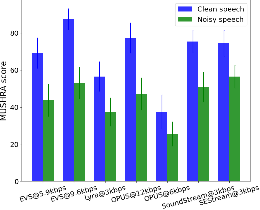


We further compare our method with other representative audio codecs, including Lyra, EVS, and OPUS at various bit-rates. We compare the methods on 20 examples for each case of low bit-rate and medium bit-rate, which contain clean test set and noisy test set with SNRs ranging from 0 dB to 15 dB uniformly. The subjective quality score based on MUSHRA is shown in Fig. 3. Details are shown in Fig. 4. It can be seen that at low and medium bit-rates, our method achieves a performance comparable with SoundStream in terms of subjective quality score with a slight advantage. Using a low bit-rate, e.g., 3 kbps, SoundStream and SEStream can achieve scores close to that of EVS at a higher bit-rate, e.g., 9.6 kbps, while outperforming OPUS at a higher bit-rate of 12 kbps.
As can be seen from Fig. 4, the perceptual quality of our proposed method on clean speech is similar to that of SoundStream, and the advantage is in noisy speech at a low bit-rate. Compared with other codecs, it is obvious that the joint speech compression and enhancement has better perceptual quality on noisy speech.
Fig. 5 compares the subjective quality score in the cases of low bit-rate and high noise with 0 dB and 10 dB SNR. In these cases, the performance of traditional codecs deteriorates drastically. In comparison, the advantage of SoundStream and SEStream over other codecs is more conspicuous, reflecting the better performance of SoundStream and SEStream in the presence of noise.
Table II compares the codecs in terms of the objective metric ViSQOL. We select 200 examples for the clean test set and 200 examples for the noisy test set (with SNRs ranging from 0 dB to 15 dB). SEStream has better ViSQOL scores than SoundStream, indicating that the distortion of SEStream is lower. Although the denoised results of Lyra sound relatively natural, there exists more serious distortion in timbre, thus, with significantly worse ViSQOL scores.
| Clean | Noisy | |
| Lyra @3 kbps | 2.43 | 2.37 |
| EVS @5.9 kbps | 2.46 | 2.40 |
| EVS @9.6 kbps | 3.90 | 3.50 |
| EVS @13.2 kbps | 3.94 | 3.61 |
| OPUS @6 kbps | 2.13 | 2.07 |
| OPUS @12 kbps | 2.68 | 2.56 |
| OPUS @16 kbps | 4.11 | 3.64 |
| SoundStream @3 kbps | 3.91 | 3.66 |
| SoundStream @6 kbps | 4.05 | 3.76 |
| SEStream @3 kbps | 4.00 | 3.71 |
| SEStream @6 kbps | 4.12 | 3.82 |

Noisy speech


Clean speech


SoundStream


SEStream


VI Conclusions
In this paper, a theoretical result is derived for the joint compression and enhancement problem for speech signal in the presence of background noise. Based on the result, a two-stage training method for joint speech compression and enhancement has been proposed. Extensive experimental results on various bit-rate and noise conditions demonstrated that, the proposed method can achieve better performance in comparison with state-of-the-art codecs in terms of both objective and subjective metrics. The advantage of the proposed method is more distinct in the case of low bit-rate and high noise.
References
- [1] M. Neuendorf, M. Multrus, N. Rettelbach, G. Fuchs, J. Robilliard, J. Lecomte, S. Wilde, S. Bayer, S. Disch, C. Helmrich et al., “The iso/mpeg unified speech and audio coding standard—consistent high quality for all content types and at all bit rates,” Journal of the Audio Engineering Society, vol. 61, no. 12, pp. 956–977, 2013.
- [2] J.-M. Valin, K. Vos, and T. Terriberry, “Definition of the opus audio codec,” IETF RFC, vol. 6716, pp. 1–326, 2012.
- [3] M. Dietz, M. Multrus, V. Eksler, V. Malenovsky, E. Norvell, H. Pobloth, L. Miao, Z. Wang, L. Laaksonen, A. Vasilache et al., “Overview of the evs codec architecture,” in IEEE International Conference on Acoustics, Speech and Signal Processing (ICASSP), 2015, pp. 5698–5702.
- [4] X. Jiang, X. Peng, C. Zheng, H. Xue, Y. Zhang, and Y. Lu, “End-to-end neural speech coding for real-time communications,” in IEEE International Conference on Acoustics, Speech and Signal Processing (ICASSP), 2022, pp. 866–870.
- [5] A. Omran, N. Zeghidour, Z. Borsos, F. d. C. Quitry, M. Slaney, and M. Tagliasacchi, “Disentangling speech from surroundings in a neural audio codec,” arXiv preprint arXiv:2203.15578, 2022.
- [6] W. B. Kleijn, A. Storus, M. Chinen, T. Denton, F. S. C. Lim, A. Luebs, J. Skoglund, and H. Yeh, “Generative speech coding with predictive variance regularization,” in IEEE International Conference on Acoustics, Speech and Signal Processing (ICASSP), 2021, pp. 6478–6482.
- [7] S. Sonning, C. Schüldt, H. Erdogan, and S. Wisdom, “Performance study of a convolutional time-domain audio separation network for real-time speech denoising,” in IEEE International Conference on Acoustics, Speech and Signal Processing (ICASSP), 2020, pp. 831–835.
- [8] N. Zeghidour, A. Luebs, A. Omran, J. Skoglund, and M. Tagliasacchi, “Soundstream: An end-to-end neural audio codec,” IEEE/ACM Transactions on Audio, Speech, and Language Processing, vol. 30, pp. 495–507, 2021.
- [9] A. Razavi, A. Van den Oord, and O. Vinyals, “Generating diverse high-fidelity images with vq-vae-2,” Advances in neural information processing systems, vol. 32, 2019.
- [10] E. Perez, F. Strub, H. De Vries, V. Dumoulin, and A. Courville, “Film: Visual reasoning with a general conditioning layer,” in Proceedings of the AAAI Conference on Artificial Intelligence, 2018.
- [11] Y. Blau and T. Michaeli, “The perception-distortion tradeoff,” in Proceedings of the IEEE Conference on Computer Vision and Pattern Recognition, 2018, pp. 6228–6237.
- [12] J. Kong, J. Kim, and J. Bae, “Hifi-gan: Generative adversarial networks for efficient and high fidelity speech synthesis,” Advances in Neural Information Processing Systems, vol. 33, pp. 17 022–17 033, 2020.
- [13] Z. Yan, F. Wen, R. Ying, C. Ma, and P. Liu, “On perceptual lossy compression: The cost of perceptual reconstruction and an optimal training framework,” in International Conference on Machine Learning, 2021, pp. 11 682–11 692.
- [14] Z. Yan, F. Wen, and P. Liu, “Optimally controllable perceptual lossy compression,” in International Conference on Machine Learning, 2022, pp. 24 911–24 928.
- [15] H. Zen, V. Dang, R. Clark, Y. Zhang, R. J. Weiss, Y. Jia, Z. Chen, and Y. Wu, “Libritts: A corpus derived from librispeech for text-to-speech,” in Interspeech, 2019, pp. 1526–1530.
- [16] E. Fonseca, J. Pons Puig, X. Favory, F. Font Corbera, D. Bogdanov, A. Ferraro, S. Oramas, A. Porter, and X. Serra, “Freesound datasets: A platform for the creation of open audio datasets,” in International Society for Music Information Retrieval Conference, 2017.
- [17] R. B. ITU, “Method for the subjective assessment of intermediate quality levels of coding systems,” Recommendation ITU-R BS. 1534, 2001.
- [18] A. Hines, J. Skoglund, A. Kokaram, and N. Harte, “Visqol: The virtual speech quality objective listener,” in International Workshop on Acoustic Signal Enhancement, 2012, pp. 1–4.
- [19] K. Kumar, R. Kumar, T. de Boissière, L. Gestin, W. Z. Teoh, J. M. R. Sotelo, A. de Brébisson, Y. Bengio, and A. C. Courville, “Melgan: Generative adversarial networks for conditional waveform synthesis,” Advances in neural information processing systems, vol. 32, 2019.
- [20] A. Vasuki and P. Vanathi, “A review of vector quantization techniques,” IEEE Potentials, vol. 25, no. 4, pp. 39–47, 2006.
- [21] C. H. Taal, R. C. Hendriks, R. Heusdens, and J. Jensen, “A short-time objective intelligibility measure for time-frequency weighted noisy speech,” in IEEE International Conference on Acoustics, Speech and Signal Processing, 2010, pp. 4214–4217.
- [22] A. van den Oord, S. Dieleman, H. Zen, K. Simonyan, O. Vinyals, A. Graves, N. Kalchbrenner, A. Senior, and K. Kavukcuoglu, “Wavenet: A generative model for raw audio,” in 9th ISCA Speech Synthesis Workshop, 2016, p. 125.
- [23] Y. Blau and T. Michaeli, “Rethinking lossy compression: The rate-distortion-perception tradeoff,” in International Conference on Machine Learning, 2019, pp. 675–685.
- [24] N. Kalchbrenner, E. Elsen, K. Simonyan, S. Noury, N. Casagrande, E. Lockhart, F. Stimberg, A. Oord, S. Dieleman, and K. Kavukcuoglu, “Efficient neural audio synthesis,” in International Conference on Machine Learning, 2018, pp. 2410–2419.
- [25] A. Gritsenko, T. Salimans, R. van den Berg, J. Snoek, and N. Kalchbrenner, “A spectral energy distance for parallel speech synthesis,” Advances in Neural Information Processing Systems, vol. 33, pp. 13 062–13 072, 2020.
- [26] W. B. Kleijn, F. S. Lim, A. Luebs, J. Skoglund, F. Stimberg, Q. Wang, and T. C. Walters, “Wavenet based low rate speech coding,” in IEEE International Conference on Acoustics, Speech and Signal Processing (ICASSP), 2018, pp. 676–680.
- [27] J. Klejsa, P. Hedelin, C. Zhou, R. Fejgin, and L. Villemoes, “High-quality speech coding with sample rnn,” in IEEE International Conference on Acoustics, Speech and Signal Processing (ICASSP), 2019, pp. 7155–7159.
- [28] R. Fejgin, J. Klejsa, L. Villemoes, and C. Zhou, “Source coding of audio signals with a generative model,” in IEEE International Conference on Acoustics, Speech and Signal Processing (ICASSP), 2020, pp. 341–345.
- [29] J. Skoglund and J.-M. Valin, “Improving opus low bit rate quality with neural speech synthesis,” in Interspeech, 2019, pp. 2847–2851.
- [30] J.-M. Valin and J. Skoglund, “Lpcnet: Improving neural speech synthesis through linear prediction,” in IEEE International Conference on Acoustics, Speech and Signal Processing (ICASSP), 2019, pp. 5891–5895.
- [31] C. Gârbacea, A. v. den Oord, Y. Li, F. S. C. Lim, A. Luebs, O. Vinyals, and T. C. Walters, “Low bit-rate speech coding with vq-vae and a wavenet decoder,” in IEEE International Conference on Acoustics, Speech and Signal Processing (ICASSP), 2019, pp. 735–739.
- [32] J. Williams, Y. Zhao, E. Cooper, and J. Yamagishi, “Learning disentangled phone and speaker representations in a semi-supervised vq-vae paradigm,” in IEEE International Conference on Acoustics, Speech and Signal Processing (ICASSP), 2021, pp. 7053–7057.
- [33] K. Zhen, J. Sung, M. S. Lee, S. Beack, and M. Kim, “Cascaded cross-module residual learning towards lightweight end-to-end speech coding,” in Interspeech, 2019.
- [34] A. Van Den Oord, O. Vinyals et al., “Neural discrete representation learning,” Advances in neural information processing systems, vol. 30, 2017.
- [35] X. Feng, Y. Zhang, and J. R. Glass, “Speech feature denoising and dereverberation via deep autoencoders for noisy reverberant speech recognition,” in IEEE International Conference on Acoustics, Speech and Signal Processing (ICASSP), 2014, pp. 1759–1763.
- [36] S. Pascual, A. Bonafonte, and J. Serrà, “Segan: Speech enhancement generative adversarial network,” in Interspeech, 2017, pp. 3642–3646.
- [37] F. G. Germain, Q. Chen, and V. Koltun, “Speech denoising with deep feature losses,” in Interspeech, 2019, pp. 2723–2727.
- [38] D. Rethage, J. Pons, and X. Serra, “A wavenet for speech denoising,” in IEEE International Conference on Acoustics, Speech and Signal Processing (ICASSP), 2017, pp. 5069–5073.
- [39] T. Ishii, H. Komiyama, T. Shinozaki, Y. Horiuchi, and S. Kuroiwa, “Reverberant speech recognition based on denoising autoencoder,” in Interspeech, 2013.
- [40] D. S. Williamson and D. Wang, “Time-frequency masking in the complex domain for speech dereverberation and denoising,” IEEE/ACM Transactions on Audio, Speech, and Language Processing, vol. 25, pp. 1492–1501, 2017.
- [41] A. Biswas and D. Jia, “Audio codec enhancement with generative adversarial networks,” in IEEE International Conference on Acoustics, Speech and Signal Processing (ICASSP), 2020, pp. 356–360.
- [42] Y. Li, M. Tagliasacchi, O. Rybakov, V. Ungureanu, and D. Roblek, “Real-time speech frequency bandwidth extension,” in IEEE International Conference on Acoustics, Speech and Signal Processing (ICASSP), 2020, pp. 691–695.
- [43] T.-Y. Lim, R. A. Yeh, Y. Xu, M. N. Do, and M. A. Hasegawa-Johnson, “Time-frequency networks for audio super-resolution,” in IEEE International Conference on Acoustics, Speech and Signal Processing (ICASSP), 2018, pp. 646–650.
- [44] S.-W. Fu, T.-W. Wang, Y. Tsao, X. Lu, and H. Kawai, “End-to-end waveform utterance enhancement for direct evaluation metrics optimization by fully convolutional neural networks,” IEEE/ACM Transactions on Audio, Speech, and Language Processing, vol. 26, pp. 1570–1584, 2017.
- [45] Y. Koizumi, K. Niwa, Y. Hioka, K. Kobayashi, and Y. Haneda, “Dnn-based source enhancement to increase objective sound quality assessment score,” IEEE/ACM Transactions on Audio, Speech, and Language Processing, vol. 26, pp. 1780–1792, 2018.
- [46] S.-W. Fu, C.-F. Liao, Y. Tsao, and S.-D. Lin, “Metricgan: Generative adversarial networks based black-box metric scores optimization for speech enhancement,” in International Conference on Machine Learning, 2019, pp. 2031–2041.
- [47] M. H. Soni, N. Shah, and H. A. Patil, “Time-frequency masking-based speech enhancement using generative adversarial network,” in IEEE International Conference on Acoustics, Speech and Signal Processing (ICASSP), 2018, pp. 5039–5043.
- [48] Y.-J. Lu, Z. Wang, S. Watanabe, A. Richard, C. Yu, and Y. Tsao, “Conditional diffusion probabilistic model for speech enhancement,” in IEEE International Conference on Acoustics, Speech and Signal Processing (ICASSP), 2022, pp. 7402–7406.
- [49] C. Donahue, J. McAuley, and M. Puckette, “Adversarial audio synthesis,” in International Conference on Learning Representations, 2018.
- [50] R. Yamamoto, E. Song, and J.-M. Kim, “Parallel wavegan: A fast waveform generation model based on generative adversarial networks with multi-resolution spectrogram,” in IEEE International Conference on Acoustics, Speech and Signal Processing (ICASSP), 2019, pp. 6199–6203.
- [51] J.-H. Kim, S.-H. Lee, J.-H. Lee, and S.-W. Lee, “Fre-gan: Adversarial frequency-consistent audio synthesis,” in Interspeech, 2021.
- [52] J. Casebeer, V. Vale, U. Isik, J.-M. Valin, R. Giri, and A. Krishnaswamy, “Enhancing into the codec: Noise robust speech coding with vector-quantized autoencoders,” in IEEE International Conference on Acoustics, Speech and Signal Processing (ICASSP), 2021, pp. 711–715.
- [53] W. Jiang, T. Liu, and K. Yu, “Efficient speech enhancement with neural homomorphic synthesis,” in Interspeech, 2022, pp. 986–990.
- [54] W. Jiang, Z. Liu, K. Yu, and F. Wen, “Speech enhancement with neural homomorphic synthesis,” in IEEE International Conference on Acoustics, Speech and Signal Processing (ICASSP), 2022, pp. 376–380.
- [55] J. Lin, K. Kalgaonkar, Q. He, and X. Lei, “Speech enhancement for low bit rate speech codec,” in IEEE International Conference on Acoustics, Speech and Signal Processing (ICASSP), 2022, pp. 7777–7781.
- [56] Y. Chen, S. Yang, N. Hu, L. Xie, and D. Su, “Tenc: Low bit-rate speech coding with vq-vae and gan,” in International Conference on Multimodal Interaction, 2021.
- [57] A. van den Oord, Y. Li, I. Babuschkin, K. Simonyan, O. Vinyals, K. Kavukcuoglu, G. van den Driessche, E. Lockhart, L. C. Cobo, F. Stimberg, N. Casagrande, D. Grewe, S. Noury, S. Dieleman, E. Elsen, N. Kalchbrenner, H. Zen, A. Graves, H. King, T. Walters, D. Belov, and D. Hassabis, “Parallel wavenet: Fast high-fidelity speech synthesis,” in Proceedings of the 35th International Conference on Machine Learning, 2017, p. 3918–3926.
- [58] C. Donahue, B. Li, and R. Prabhavalkar, “Exploring speech enhancement with generative adversarial networks for robust speech recognition,” in IEEE International Conference on Acoustics, Speech and Signal Processing (ICASSP), 2017, pp. 5024–5028.
- [59] S. F. Boll, “Suppression of acoustic noise in speech using spectral subtraction,” IEEE/ACM Transactions on Acoustics, Speech, and Signal Processing, vol. 27, pp. 113–120, 1979.
- [60] M. G. Berouti, R. M. Schwartz, and J. Makhoul, “Enhancement of speech corrupted by acoustic noise,” in IEEE International Conference on Acoustics, Speech, and Signal Processing, 1979.
- [61] Y. Ephraim and H. L. V. Trees, “A signal subspace approach for speech enhancement,” in IEEE International Conference on Acoustics, Speech, and Signal Processing, 1993, pp. 355–358.
- [62] R. Dobrushin and B. Tsybakov, “Information transmission with additional noise,” IRE Trans. Inf. Theory, vol. 8, no. 5, pp. 293–304, 1962.
- [63] J. Wolf and J. Ziv, “Transmission of noisy information to a noisy receiver with minimum distortion,” IEEE Trans. Inf. Theory, vol. 16, no. 4, pp. 406–411, 1970.