A two-piece property for free boundary minimal hypersurfaces in the -dimensional ball
Abstract.
We prove that every hyperplane passing through the origin in divides an embedded compact free boundary minimal hypersurface of the euclidean -ball in exactly two connected hypersurfaces. We also show that if a region in the -ball has mean convex boundary and contains a nullhomologous -dimensional equatorial disk, then this region is a closed halfball. Our first result gives evidence to a conjecture by Fraser and Li in any dimension.
1. Introduction
Inspired by the work of Ros [26] for closed minimal surfaces in , the authors proved in [25] the two-piece property for free boundary minimal surfaces in the unit ball of . This result gives evidence to a conjecture by Fraser and Li [10] concerning the first Steklov eigenvalue of free boundary minimal surfaces in Also, Kusner and McGrath [21] used our result of two-piece property in the free boundary context to prove the uniqueness of the critical catenoid among embedded minimal annuli invariant under the antipodal map. This settles a case of another well-known conjecture of [10] on the uniqueness of the critical catenoid.
In the present paper we prove that the two-piece property holds in any dimension. More precisely, we prove the following.
Theorem A (The two-piece property).
Every hyperplane in passing through the origin divides an embedded compact free boundary minimal hypersurface of the unit -ball in exactly two connected components.
We also prove the following result which can be seen as a strong version of the analog of the result by Solomon [29] in the free boundary context.
Theorem B.
Let be a connected closed region with mean convex boundary such that meets orthogonally along its boundary and is smooth. Suppose contains a set of the form which is nullhomologous in (see Definition 3), where is a -dimensional plane in passing through the origin. Then is a closed halfball.
Let us remark that exactly as in the case , Theorem A can be proved by assuming the conjecture by Fraser and Li [10] on the the first Steklov eigenvalue of free boundary minimal hypersurfaces in ; hence, Theorem A gives evidence to this conjecture (see [25, Remark 2]).
The strategy to prove Theorem A and Theorem B is similar to the case and uses Geometric Measure Theory to analyze the minimizers of a partially free boundary problem for the area functional. However, in higher dimensions the situation is more delicate since the hypersurfaces obtained as minimizers can have a singular set (see Theorem 1).
Motivated mainly by the celebrated work of Fraser and Schoen [11, 12], the study of free boundary minimal surfaces in saw a rapid development in the last few years, see for instance [22] and the references therein. However, the case of free boundary minimal hypersurfaces in is not so well-studied. Concerning examples, some free boundary minimal hypersurfaces with symmetry were constructed in [14], and a variational theory has been developed in [23, 31, 32].
Regarding some properties of free boundary minimal hypersurfaces, we can mention that the asymptotic properties of the index of higher-dimensional free boundary minimal catenoids were studied in [28], and in [1] it was proved that the index of a properly embedded free boundary minimal hypersurface in grows linearly with the dimension of its first relative homology group. In [24] the first author proved the index can be controlled from above by a function of the norm of the second fundamental form. Also, compactness results for the space of free boundary minimal hypersurfaces were obtained in [10, 2, 17].
2. Preliminary
2.1. Free boundary minimal hypersurfaces
Let be the unit ball of dimension with boundary . Throughout this paper we will denote by the dimensional equatorial disk which is the intersection of with a hyperplane passing through the origin. In the following, denotes the -dimensional Hausdorff measure, where .
Let . Along this section we will use the following notation/assumptions:
-
•
is compact and it is contained in .
-
•
is an embedded orientable smooth hypersurface with boundary.
-
•
The singular set is the complement of in . We suppose .
-
•
The boundary of satisfies , where and We have that, away from the singular set, is an embedded smooth submanifold of dimension .
Definition 1.
Let be as above. We say that is a minimal hypersurface with free boundary if the mean curvature vector of vanishes and meets orthogonally along (in particular, We say that is a minimal hypersurface with partially free boundary if the mean curvature vector of vanishes and its boundary satisfies that and meets orthogonally along .
From now on, given a (partially) free boundary minimal hypersurface with boundary , we will call its fixed boundary and its free boundary.
Definition 2.
Let be a partially free boundary minimal hypersurface in . We say that is stable if for any function such that and is away from the singular set , we have
| (2.1) |
or equivalently
| (2.2) |
where is the outward normal vector field to .
Observe that if is stable then, by an approximation argument, the inequality (2.2) holds for any function such that for a.e. and is away from the singular set. In particular (2.2) holds for any Lipschitz function satisfying the boundary condition.
Lemma 1.
Let be a partially free boundary minimal hypersurface in of finite area and such that the singular set satisfies , where and . If is contained in an n-dimensional equatorial disk, then is totally geodesic.
Proof.
Let be as in the hypotheses and denote by the equatorial disk that contains . Let be a vector orthogonal to the disk and consider the function , By hypothesis, we know that . A standard calculation using that is minimal and free boundary yields
Fix and consider a smooth function so that
-
•
for ,
-
•
for ,
-
•
, for some constant .
Define as . In particular, we have in Observe that the set where is not smooth satisfies
Since is compact and , for any there exist balls such that
For each , consider a smooth function such that
-
•
in ,
-
•
in ,
-
•
.
Define by , where and . We have that is Lipschitz and , hence (2.2) holds. Moreover
and
since , and Hence, applying it to (2.2), we get
| (2.3) |
On the other hand, along we have . Since has support away from the singular set, by the classical monotonicity formula at the interior and at the free boundary, there is such that
Thus
If we let first and then we obtain
If then is totally geodesic and we are done. If for some then we can find a neighborhood of in such that is strictly positive. This implies for any . Therefore, is entirely contained in the disk in particular, it is totally geodesic. ∎
An equatorial disk divides the ball into two (open) halfballs. We will denote these two halfballs by and and we have
In the next proposition we will summarize some facts about partially free boundary minimal surfaces in which we will use in the proof of Theorem 3.
Proposition 1.
-
(i)
Let be an equatorial disk and let be a smooth partially free boundary minimal hypersurface in contained in one of the closed halfballs determined by , say and such that . If is not contained in an equatorial disk, then has necessarily nonempty fixed boundary and nonempty free boundary.
-
(ii)
The only smooth (partially) free boundary minimal hypersurface that contains a -dimensional piece of the free boundary of a dimensional equatorial disk is (contained in) this equatorial disk itself.
Proof.
If the free boundary were empty, we could apply the (interior) maximum principle with the family of hyperplanes parallel to the disk and conclude that should be contained in the disk . On the other hand, if the fixed boundary were empty, then we would have a minimal hypersurface entirely contained in a halfball without fixed boundary; hence, we could apply the (interior or free boundary version of) maximum principle with the family of equatorial disks that are rotations of around a dimensional equatorial disk and conclude that should be an equatorial disk.
Let be an equatorial disk and suppose that is a (partially) free boundary minimal hypersurface such that contains a dimensional piece of the free boundary of in Assume, without loss of generality, .
Observe that since is free boundary we know that where is the conormal vector to and since is a minimal hypersurface in we have that is harmonic.
We will show that
Consider an extension of along such that and define on as
Observe that , and where is the conormal to pointing towards and is the conormal to pointing towards hence, is in a neighborhood of in
Claim 1.
is a weak solution to the Laplacian equation
Observe that is a harmonic function on , so we just need to show the claim in a neighborhood of
Consider a domain where with and (see Figure 1), and let be a smooth function with compact support contained in
Integration by parts gives us
since supp where is the outward conormal to
Then,
We have
where in the first equality we used that and in the second equality we used the fact that where is the outward conomal to with respect to
Analogously, we have
where in the first equality we used that is harmonic and in the second equality we used the fact that where is the outward conomal to with respect to
Therefore, the claim follows and, by the Elliptic theory, has to be a (strong) solution to the Laplacian equation. Moreover, since vanishes on an open set, the unique continuation result implies that on that is, is (contained in) the equatorial disk ∎
2.2. Integer rectifiable varifolds
A set is called countably -rectifiable if is -measurable and if
where and for , is an -dimensional -submanifold of . Such possesses -a.e. an approximate tangent space .
Let be the Grassmannian of -hyperplanes in . An integer multiplicity rectifiable -varifold is a Radon measure on , defined by
where is countably -rectifiable and is a locally -integrable integer valued function. Also, we say is stationary if
| (2.4) |
for any -vector field of compact support.
Then we have the following result, see [20].
Lemma 2.
Let be an embedded -hypersurface such that , for every open set with compact closure. Let be a integer valued function which is locally constant. Then, the following conditions are equivalent:
-
(1)
is stationary.
-
(2)
, and there is such that for any ball we have
2.3. Minimizing Currents with Partially Free Boundary
In this section we will use the following notation.
-
•
is an open set;
-
•
;
-
•
denotes the dual of , and its elements are called -currents with support in ;
-
•
The mass of in is defined by
-
•
The boundary of is the -current given by
where denotes the exterior derivative operator.
Consider a compact domain such that , where is a compact hypersurface (not necessarily connected) with boundary, is a smooth compact mean convex hypersurface with boundary, which intersects orthogonally along , and such that .
Let be a compact hypersurface with boundary . We assume that is an embedded -submanifold of dimension away from a singular set such that .
Define the class of admissible currents by
where is the current associated to with multiplicity one. We want to minimize area in , that is, we are looking for such that
| (2.5) |
Observe that since . Hence, it follows from [8, ], that the variational problem (2.5) has a solution (see also [15]). If is a solution we have
| (2.6) | |||||
| (2.7) | |||||
| (2.8) |
for any integer multiplicity current with compact support such that and .
In order to apply the known regularity theory for we need the following result, whose proof is the same as that of the case (see Section 3 in [25]).
Proposition 2.
If is a solution of (2.5), then either or .
For any given dimensional compact set we call corners the set of points of which also belong to . We then have the following regularity result.
Theorem 1.
Let be a solution of (2.5). Then there is a set such that, away from , is supported in a oriented embedded minimal -hypersurface, which meets orthogonally along . Moreover
| (2.9) |
Proof.
Let us write
where the union is disjoint and consists of the points such that there is a neighborhood of where is given by -times () integration over an embedded -hypersurface with boundary. To complete the proof we will prove the following:
3. The two-piece property and other results
Definition 3.
Let be a region in and let be a dimensional equatorial disk (that is, the intersection of with an -dimensional plane passing through the origin). We say that is nullhomologous in if there exists a compact hypersurface such that , where is a dimensional compact set contained in (see Figure 2).
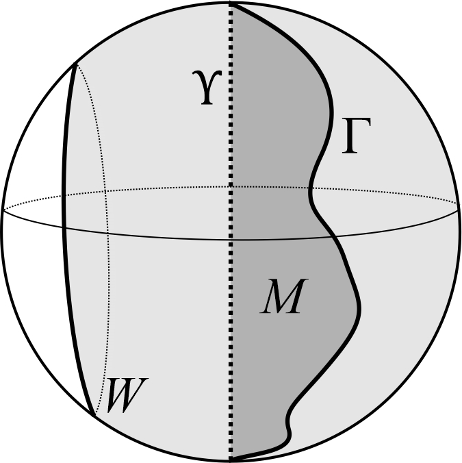
The boundary of the region can be written as , where and In the next theorem we will denote by the closure of the component that is,
Theorem 2.
Let be a connected closed region with (not necessarily strictly) mean convex boundary such that meets orthogonally along its boundary and is smooth. If contains a dimensional equatorial disk , and is nullhomologous in , then is a closed -dimensional halfball.
Proof.
Up to a rotation of around the origin, we can assume that is nonempty. Since is nullhomologous in , there exists a compact hypersurface contained in such that , where is a dimensional compact set contained in We consider the class of admissible currents
where is the current associated to with multiplicity one, and we minimize area (mass) in Then, by the results presented in Section 2.3, we get a compact embedded (orientable) partially free boundary minimal hypersurface which minimizes area among compact hypersurfaces in with boundary on the class in particular, its fixed boundary is exactly Moreover, by Proposition 2 in Section 2.3, either or
Now the same arguments we used in the proof of Theorem 1 in [25] can be applied. In fact:
Claim 2.
is stable.
In the case , is automatically stable in the sense of Definition 2, since it minimizes area for all local deformations.
Suppose . For any with , consider defined by
and let be a first eigenfunction, i.e., .
Observe that although differently from the classical stability quotient (we have an extra term that depends on the boundary of ) we can still guarantee the existence of a first eigenfunction. In fact, since for any there exists such that , for any , we can use this inequality to prove that the infimum is finite. Once this is established the classical arguments to show the existence of a first eigenfunction work.
Since a.e., we have , that is, is also a first eigenfunction. Since , the maximum principle implies that in , in particular, does not change sign in . Then we can assume that in and, by continuity, we get in Therefore, we can use as a test function to our variational problem: Let be a smooth vector field such that for all , for all , and points towards along . Let be the flow of . For small enough the hypersurfaces ; , are contained in . Since has least area among the hypersurfaces , we know that
which implies that . Since is a first eigenfunction, we get that for any with . Therefore, we have stability for .
Then, since is contained in an equatorial disk , Lemma 1 implies that is necessarily a half dimensional equatorial disk. If , then we already conclude that has to be a dimensional halfball.
Suppose . Rotate around until the last time it remains in (this last time exists once is nonempty), and let us still denote this rotated hypersurface by . In particular, there exists a point where and are tangent. We will conclude that is necessarily a dimensional halfball.
In fact, if we can write locally as a graph over around and apply the classical Hopf Lemma; if we can use the Serrin’s Maximum Principle at a corner (see Appendix A in [25] for the details); and if we can apply (the interior or the free boundary version of) the maximum principle. In any case, we get that is a dimensional halfball. ∎
Now we prove the two-piece property for free boundary minimal hypersurfaces in .
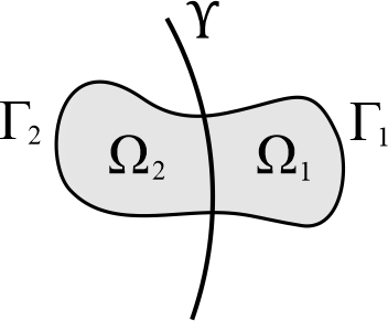
Theorem 3.
Let be a compact embedded smooth free boundary minimal hypersurface in Then for any equatorial disk , and are connected.
Proof.
If is an equatorial disk, then the result is trivial. So let us assume this is not the case.
Suppose that, for some equatorial disk , is a disjoint union of two nonempty open hypersurfaces and , being connected. Notice that by Proposition 1(i) both and (all components of) have nonempty fixed boundary and nonempty free boundary. Let us denote by the fixed boundary of which might be disconnected. If and are transverse, then is an embedded smooth submanifold of dimension . If and are tangent, then the local description of nodal sets of elliptic PDE’s (see for instance [19]) imply that is an embedded smooth submanifold of dimension , away from a singular set such that .
Denote by and the closures of the two components of They are compact domains with mean convex boundary. Hence, we can minimize area for the following partially free boundary problem (see Section 2.3):
We consider the class of admissible currents
where is the current associated to with multiplicity one, and we minimize area (mass) in Then, by the results presented in Section 2.3, we get a compact embedded (orientable) partially free boundary minimal hypersurface which minimizes area among compact hypersurfaces in with the same fixed boundary as , which is contained in Moreover, by Proposition 2 in Section 2.3, either or
Arguing as in Claim 2 of Theorem 2, we can prove the stability of . Also, observe that by Theorem 1 the singular set of is empty or satisfies , in particular . So, we can apply Lemma 1 and conclude that each component of is a piece of an equatorial disk.
The case can not happen because this would imply that is a disk, and we are assuming it is not. Therefore, only the second case can happen, that is, any component of meets only at points of Observe that each component of that is not bounded by a dimensional equatorial disk is necessarily contained in . If some component of were bounded by a dimensional equatorial disk, then we could apply Theorem 2 and would conclude that is a dimensional equatorial disk, which is not the case. Then is entirely contained in and, since , and does not contain any -dimensional piece of (Proposition 1(ii)), we have .
Doing the same procedure as in the last paragraph for , we can construct another compact hypersurface of with fixed boundary and such that and . Notice that is a hypersurface without fixed boundary of , therefore In fact, let us denote by and the minimizing currents associated to and respectively, that is, and . First observe that and ; hence, by the Constancy Theorem, we know that , for some interger . Now, since and the Constancy Theorem implies that ; but since has multiplicity one, this also holds for and and therefore necessarily. Hence, .
In particular, which implies that has fixed boundary contained in . For , since is embedded and has singularities of -prong type (if any), we know that the fixed boundaries of and are disjoint, in particular, the fixed boundary of is necessarily empty and this yields a contradiction by Proposition 1(i). It remains to analyse the case when
Let us assume, without loss of generality, that ; hence, we have which is the nodal set of the Steklov eigenfunction
Observe that if and then, since is embedded, we know that in a neighborhood of we have ; in particular, can not be contained in
Now let us analyse the singular set By Theorem 1.7 in [19], the Hausdorff dimension of is less than or equal to in particular, and therefore by Lemma 2 is stationary. By [30] we can conclude that either or (which we already know is not possible). Therefore, has empty fixed boundary which is a contradiction by Proposition 1(i).
Therefore, the theorem is proved. ∎
References
- [1] L. Ambrozio, A. Carlotto and B. Sharp, Index estimates for free boundary minimal hypersurfaces, Math. Ann. 370 (2018), 1063–1078.
- [2] L. Ambrozio, A. Carlotto and B. Sharp, Compactness analysis for free boundary minimal hypersurfaces, Calc. Var. Partial Differential Equations 57 (2018), no. 1, Art. 22, 39 pp.
- [3] W. K. Allard, On the first variation of a varifold, Ann. of Math. 95 (1972), no. 3, 417–491.
- [4] W. K. Allard, On the first variation of a varifold: boundary behavior, Ann. of Math. 101 (1975), no. 3, 418–446.
- [5] T. Bourni, Allard-type boundary regularity for boundaries, Adv. Calc. Var. 9 (2016), no. 2, 143–161.
- [6] F. Duzaar and K. Steffan, Optimal interior and boundary regularity for almost minimizers to elliptic variational integrals, J. Reine Angew. Math. 546 (2002), 73–138.
- [7] N. Edelen, A note on the singular set of area-minimizing hypersurfaces, Calc. Var. Partial Differential Equations 59 (2020), no. 1, Art. 18, 9 pp.
- [8] H. Federer, Geometric measure theory, Grundlehren der math. Wiss. 153. Springer, New York 1969.
- [9] H. Federer, The singular sets of area minimizing rectifiable currents with codimension one and of area minimizing flat chains modulo two with arbitrary codimension, Bull. Amer. Math. Soc. 76 (1970), 767–771.
- [10] A. Fraser and M. Li, Compactness of the space of embedded minimal surfaces with free boundary in three-manifolds with nonnegative Ricci curvature and convex boundary, J. Differential Geom. 96 (2014), 183–200.
- [11] A. Fraser and R. Schoen, The first Steklov eigenvalue, conformal geometry, and minimal surfaces, Adv. Math. 226 (2011), no. 5, 4011–4030.
- [12] A. Fraser and R. Schoen, Minimal surfaces and eigenvalue problems, Contemp. Math. 599 (2013), 105–121.
- [13] A. Fraser and R. Schoen, Sharp eigenvalue bounds and minimal surfaces in the ball, Invent. Math. 203 (2016), no. 3, 823–890.
- [14] B. Freidin, M. Gulian and P. McGrath, Free boundary minimal surfaces in the unit ball with low cohomogeneity, Proc. Amer. Math. Soc. 145 (2017), no. 4, 1671–1683.
- [15] M. Grüter, Regularitt von minimierenden Strömen bei einer freien Randbedingung, Universitt Düsseldorf, 1985.
- [16] M. Grüter, Optimal regularity for codimension one minimal surfaces with a free boundary, Manuscripta Math. 58 (1987), no. 3, 295–343.
- [17] Q. Guang, X. Zhou. Compactness and generic finiteness for free boundary minimal hypersurfaces. Pacific J. Math. 310 (2021), no. 1, 85–114.
- [18] R. Hardt and L. Simon, Boundary regularity and embedded solutions for the oriented Plateau problem, Ann. of Math. (2) 110 (1979), no. 3, 439–486.
- [19] R. Hardt and L. Simon, Nodal sets for solutions of elliptic equations, J. Differential Geom. 30 (1989), 505–522.
- [20] T. Ilmanen, A strong maximum principle for singular minimal hypersurfaces, Calc. Var. 4 (1996), 443–467.
- [21] R. Kusner and P. McGrath, On free boundary minimal annuli embedded in the unit ball, Preprint at arXiv:2011.06884 (2020).
- [22] M. Li, Free boundary minimal surfaces in the unit ball: recent advances and open questions, Preprint at arXiv:arXiv:1907.05053v3 (2020).
- [23] M. Li and X. Zhou, Min-max theory for free boundary minimal hypersurfaces I-regularity theory, J. Differential Geom. 118 (2021), no. 3, 487–553.
- [24] V. Lima, Bounds for the Morse index of free boundary minimal surfaces, arXiv:1710.10971 to appear on Asian Journal of Mathematics.
- [25] V. Lima and A. Menezes, A two-piece property for free boundary minimal surfaces in the ball, Trans. Amer. Math. Soc., 374 (2021), no. 3, 1661–1686.
- [26] A. Ros, A two-piece property for compact minimal surfaces in a three-sphere, Indiana Univ. Math. J. 44 (1995), no. 3, 841–849.
- [27] L. Simon, Lectures on geometric measure theory, Proceedings of the Centre for Mathematical Analysis, Australian National University, vol. 3, Australian National University, Centre for Mathematical Analysis, Canberra, 1983. vii+272 pp.
- [28] G. Smith, A. Stern, H. Tran, D. Zhou, On the Morse index of higher-dimensional free boundary minimal catenoids. Calc. Var. Partial Differential Equations 60 (2021), no. 6, Paper No. 208.
- [29] B. Solomon, Harmonic maps to spheres, J. Differential Geom. 21 (1985), 151–162.
- [30] B. Solomon and B. White, A strong maximum principle for varifolds that are stationary with respect to even parametric elliptic functionals, Indiana Univ. Math. J. 38 (1989), no. 3, 683– 691.
- [31] A. Sun, Z. Wang and X. Zhou, Multiplicity one for min-max theory in compact manifolds with boundary and its applications. arXiv:2011.04136 [math.DG]
- [32] Z. Wang, Existence of infinitely many free boundary minimal hypersurfaces, Preprint at arXiv:2001.04674 (2020).