A Transfer Operator Approach to Relativistic Quantum Wavefunction

Igor Mezić
University of California, Santa Barbara, CA 93106-5070, USA
[email protected]

Abstract

The original intent of the Koopman-von Neumann formalism was to put classical and quantum mechanics on the same footing by introducing an operator formalism into classical mechanics. Here we pursue their path the opposite way and examine what transfer operators can say about quantum mechanical evolution. To that end, we introduce a physically motivated scalar wavefunction formalism for a velocity field on a 4-dimensional pseudo-Riemannian manifold, and obtain an evolution equation for the associated wavefunction, a generator for an associated weighted transfer operator. The generator of the scalar evolution is of first order in space and time. The probability interpretation of the formalism leads to recovery of the Schrödinger equation in the non-relativistic limit. In the special relativity limit, we show that the scalar wavefunction of Dirac spinors satisfies the new equation. A connection with string theoretic considerations for mass is provided.

1 Introduction

Dynamical systems theory can be pursued in the phase-space (Poincaré) formalism [1], or alternatively in the Koopman formalism [2, 3, 4]. The Koopman formalism applied in phase space leads to the probability interpretation of the associated phase-space wavefunction consistent with the Born interpretation in quantum mechanics [5]. Born’s proposal on interpretation of the square of the wavefunction as probability led to successful application of quantum mechanics to a broad swath of problems. The dichotomy between the phase-space domain of the classical wavefunction and the physical spacetime nature of the quantum wavefunction recently led to a number of efforts to reconcile the two (see e.g. [6, 7, 5, 8, 9, 10, 11, 12, 13] and the rest of the articles in this volume). These works are pursued in the nonrelativistic context. A different approach was pursued in [14], where the spectrum of the quantum harmonic oscillator was related to the Koopman operator spectrum of the classical harmonic oscillator by a construction involving a pair of harmonic oscillators with Hamiltonians of opposite sign.

In this paper we pursue the operator-theoretic approach to derive an equation of motion - the relativistic quantum transfer equation (RQTE) - for the resulting quantum-theoretical wavefunction starting from a relativistic dynamical system on a 4-dimensional space-time. Namely, we start from the spacetime manifold, and not the phase space, and utilize Fock’s proper-time formalism [15]. The key idea is that the RQTE arises from the projection of a 4-dimensional conserved field through a complex scalar field. The resulting equation - when presented in the probabilistic interpretation - has solutions that reduce to the Schrödinger equation in the nonrelativistic limit, and the euation for the Dirac scalar in the special relativity limit.

The paper is organized as follows: in section 2 we introduce the relativistic setting and the notation. In section 3 we derive RQTE under several postulates. We describe the class of operators - the weighted composition operators - that are generated by RQTE. In section 4 we discuss the relationship between RQTE and the Dirac equation. In section 5 we consider several examples treated within the RQTE formalism: harmonic oscillator, particle in a box and Gaussian wavepacket. We discuss the relationship of the RQTE wavefunction with mass in Appendix A and relationship with notion of mass in string theory in Appendix B.

2 Preliminaries

Let $M$ denote a $4$ -dimensional space-time pseudo-Riemannian manifold endowed with a metric tensor $g$ . Consider the section of its tangent bundle $TM$ , the proper velocity field (the four-velocity field) ${\bf V}=d{\bf X}/d\tau$ [16] where ${\bf X}(\tau):{\mathbb{R}}\rightarrow M$ is the time-like world line parametrized by the proper time $\tau$ . We define the level sets of proper time $\tau$ on $M$ to be able to use it for evolution of the flow of ${\bf V}$ . Any vector field on $M$ can be rectified near a point ${\bf X}$ with ${\bf V}({\bf X})\neq 0$ [17]. Since the four-velocity field ${\bf V}$ is nonzero everywhere, there exists a neighborhood $\mathscr{N}_{\bf X}$ of any point ${\bf X}$ in which it can be rectified by a local choice of coordinates $(x_{0}({\bf X}),...,x_{3}({\bf X}))$ on $M$ . In the coordinates $(x_{0},...,x_{3})$ , the four velocity field has components ${\bf V}=(c,0,0,0)$ . Note that $(x_{1},x_{2},x_{3})$ label points on the $x_{0}=0$ intersection of an individual world line. Let $\sigma=\tau(0,x_{1},x_{2},x_{3})$ be the proper time field over the section $x_{0}=0$ . We can define a new parameter $s=\tau-\sigma$ in a small neighborhood of ${\bf X}$ . In this way, the $0$ proper time is synchronized for all trajectories in a neighborhood. Absent topological obstructions, this can be extended to the whole of $M$ to define a space slice $M^{\tau}_{S}$ . With topological obstructions, the construction is still valid on subsets of $M$ . In this case, we redefine $M$ to be such a subset. We keep the notation $\tau$ for the reparametrized proper time. The norm of ${\bf V}$ defined using the metric tensor $g$ on $M$ is constant, $||{\bf V}||^{2}=-c^{2},$ where $c$ is the speed of light in vacuum [15] (we are using the $(-1,1,1,1)$ metric convention). We denote by $G^{\tau}:M\rightarrow M$ the flow of ${\bf V}$ on $M$ . We denote by $D_{\tau}f$ the proper time derivative (i.e. the Lie derivative [17]) of $f$ , representing the change of a scalar physical quantity in the direction of ${\bf V}$ . The manifold is equipped with the volume form with density $\sqrt{|\det g|}$ .

The flow $G^{\tau}$ can be used to define the family of Koopman composition operators [2] parametrized by $\tau$ acting on (in general, complex) functions $f:M\rightarrow{\mathbb{C}}$ by

{{\cal U}}^{\tau}f({\bf X})=f\circ G^{\tau}({\bf X}).

(1)

Note that, in contrast with Koopman’s original formulation on the phase space, ${\cal U}^{\tau}$ acts on functions defined on the spacetime $M$ . The operator $D_{\tau}$ is the generator of the evolution ${\cal U}^{\tau}$ . The functions in the eigenspace at $0$ of $D_{\tau}$ are conserved quantities, since

D_{\tau}f=0

(2)

implies $f$ is conserved on the world line ${\bf X}(\tau)$ . In terms of the Koopman operator evolution, for such $f$ we get

{{\cal U}}^{\tau}f({\bf X})=f({\bf X}).

(3)

In line with the terminology used in Koopman operator theory [18, 3] we call functions $g:M\rightarrow{\mathbb{C}}$ observables. By identification with the associated, position-dependent operators, the terminology is consistent with that of quantum mechanics.

3 Wavefunction Evolution

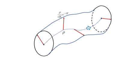
Consider a field $\rho$ conserved under trajectories of ${\bf V}$ on $M$ . Its restriction onto level sets of the complex field $e^{iY}$ of modulus $1,$ with phase $Y$ reads

\frac{\rho}{De^{iY}}=\frac{\rho}{i|DY|e^{iY}}.

(4)

We assume that the density $\rho$ is not observed directly, but is projected via a complex scalar field $e^{iY}$ , as indicated by equation (4) and shown in figure 1. The geometry can be described as that of a fiber bundle over $M$ and $\rho e^{iY}$ is a horizontal lift of the spacetime trajectory. This construction renders the appearence of complex numbers in quantum mechanics a natural consequence of geometry.

Refer to caption — Figure 1: The geometry of the fiber bundle over $M$ .

Given this geometric formulation, we use the following postulates:

3.1 Postulates

1.

There is a function $\rho:M\rightarrow{\mathbb{R}}$ that is constant on trajectories of ${\bf V}$ satisfying

$D_{\tau}\rho=0.$ (5)

We argue in the Appendix A that $\rho$ is physically the oscillation wavenumber and is related to mass (and thus energy).
2.

The observable wavefunction $\psi$ is the pushforward of $\rho$ by an observable $e^{iY}$ given by

$\psi=\frac{\rho}{i|DY|e^{iY}}=\frac{\rho}{iKe^{iY}}=\frac{\rho}{iK}e^{-iY}.$ (6)

where $Y$ is a phase and $K=|DY|$ . This, in turn, implies

$\rho=iKe^{iY}\psi.$ (7)
3.

$\rho/|DY|$ is an invariant density for ${\bf V}$ .

Remark 1.

The last postulate is natural in view of the fact that - when extending the classical action - velocity relationship relativistic, and identifying $Y$ with relativistic action, $DY$ is proportional to the space-time velocity ${\bf V}$ . Thus, the density $\rho/|DY|$ is inversely proportional to the velocity magnitude and thus is invariant.

Note that the factor $i$ is used in the wavefunction definition just for convenience of the calculations below since the constant phase of the wavefunction is irrelevant.

Under the above assumptions, we have

Theorem 1.

Let $Y=-S/\hbar,$ where $\hbar$ is the reduced Planck constant, and $D_{\tau}S={\mathscr{L}}$ , analogous to the standard notions of the action $S$ and the Lagrangian ${\mathscr{L}}$ . The wavefunction $\psi$ satisfies

i\hbar D_{\tau}\psi=-{\mathscr{L}}\psi-i\hbar{\mathsf{div}}{\bf V}\psi

(8)

where, in coordinates,

{\mathsf{div}}{\bf V}=\frac{1}{\sqrt{|}g|}\sum_{j}\frac{\partial\sqrt{|}g|V^{j}}{\partial X_{j}}

(9)

is divergence with respect to volume element, where $|g|=|\det g_{ij}|$ is the absolute value of the determinant of the metric tensor.

Proof.

By assumption 1. $D_{\tau}\rho=0$ , and we have

$\displaystyle i\hbar D_{\tau}\psi$	$\displaystyle=$	$\displaystyle-\hbar\rho\frac{D_{\tau}K}{K^{2}}e^{-iY}-i\hbar\frac{\rho}{K}D_{\tau}Ye^{-iY}$	(10)
	$\displaystyle=$	$\displaystyle-i\hbar\frac{D_{\tau}K}{K}\psi+\hbar D_{\tau}Y\psi$
	$\displaystyle=$	$\displaystyle-i\hbar\frac{D_{\tau}K}{K}\psi-{\mathscr{L}}\psi.$

Now we show that $K=|DY|$ must satisfy

D_{\tau}|DY|=|DY|{\mathsf{div}}{\bf V}.

(11)

Since $\rho/|DY|$ is an invariant density,

D_{\tau}(\rho/|DY|)=-\rho|DY|^{-2}D_{\tau}|DY|=-\rho/|DY|{\mathsf{div}}{\bf V}

(12)

implying

D_{\tau}|DY|=|DY|{\mathsf{div}}{\bf V}.

(13)

Now (10) yields

i\hbar D_{\tau}\psi=[-{\mathscr{L}}-i\hbar\ {\mathsf{div}}{\bf V}]\psi.

(14)

where $D_{\tau}$ is the proper time derivative, ${\mathscr{L}}$ is the Lagrangian, and ${\mathsf{div}}$ is the divergence of the vector field ${\bf V}$ with respect to $\sqrt{|}g|$ . ∎

It is notable that (8) has the solution

	$\displaystyle\psi({\bf Y},\tau)$	$\displaystyle=$	$\displaystyle\psi_{0}(G^{-\tau}({\bf Y}))e^{-\int_{0}^{\tau}{\mathsf{div}{\bf V}(G^{s}(G^{-\upsilon}({\bf Y})))}ds}e^{iS(\tau,{\bf Y})/\hbar},$		(15)
		$\displaystyle=$	$\displaystyle\psi_{0}({\bf X}_{0})e^{-\int_{0}^{\tau}{\mathsf{div}{\bf V}(G^{s}({\bf X}_{0}))}ds}e^{iS(\tau,{\bf Y})/\hbar},$		(15)

where $\psi({\bf Z},0)=\psi_{0}({\bf Z}),$ and ${\bf X}_{0}={\bf X}(G^{-\tau}({\bf Y}))$ is the initial position at $\tau=0$ of trajectory landing at ${\bf Y}$ at $\tau$ .

3.2 Relationship with the Schrödinger Equation

Note that for any power $(\rho/|DY|)^{\alpha}$

D_{\tau}(\rho/|DY|)^{\alpha}=-\alpha\rho^{\alpha}|DY|^{-(\alpha+1)}D_{\tau}|DY|

(16)

and thus, for $\alpha=1/2$

D_{\tau}(\rho/|DY|)^{1/2}=-\frac{1}{2}\rho^{1/2}|DY|^{-3/2}D_{\tau}|DY|=-\frac{1}{2}(\rho/|DY|)^{1/2}{\mathsf{div}}{\bf V},

(17)

where the last equation is obtained using (13). Thus, the evolution equation for

\varphi=(\rho/|DY|)^{1/2}e^{-iY}

(18)

i\hbar D_{\tau}\varphi=-{\mathscr{L}}\varphi-i\frac{\hbar}{2}{\mathsf{div}}{\bf V}\varphi,

(19)

with the solution

	$\displaystyle\varphi({\bf Y},\tau)$	$\displaystyle=$	$\displaystyle\varphi_{0}(G^{-\tau}({\bf Y}))e^{-\frac{1}{2}\int_{0}^{\tau}{\mathsf{div}{\bf V}(G^{s}(G^{-\tau}({\bf Y})))}ds}e^{iS(\tau,{\bf Y})/\hbar},$		(20)
		$\displaystyle=$	$\displaystyle\varphi_{0}({\bf X}_{0})e^{-\frac{1}{2}\int_{0}^{\tau}{\mathsf{div}{\bf V}(G^{s}({\bf X}_{0}))}ds}e^{iS(\tau,{\bf Y})/\hbar},$		(20)

Replacing $\tau$ with the classical coordinate time and assuming a flat geometry of spacetime, this solution for the wavefunction reduces to the one derived from the Schrödinger equation by Holland ([19], equation 7.3).

Remark 2.

The equation (15) can serve as a template for the path integral formulation of the current theory.

3.3 Relationship to Weighted Composition Operators

Based on (15) a group of evolution operators ${\cal W}^{\tau}$ parametrized by proper time can be defined:

{\cal W}^{\tau}\psi=\pi\cdot\psi\circ G^{-\tau}

(21)

where $\pi:M_{x}\rightarrow{\mathbb{C}}$

\pi({\bf y})=e^{-\int_{0}^{\tau}{\mathsf{div}{\bf V}(G^{s}(G^{-\tau}({\bf Y})))}ds}e^{iS(\tau,{\bf Y})/\hbar}

(22)

The operators ${\cal W}^{\tau}$ belong to the class of the so-called weighted composition operators [20].

4 Special Relativity Case: Dirac Equation

In this section we show that the scalar wave amplitude $\psi$ of a solution to Dirac equation¹¹1 $\psi$ is known to be a solution to the Klein-Gordon equation satisfies equation (8). Note here that it is only in the divergence part that the equation (8) differs from the probability amplitude equation (19), and we will see below that for Dirac equation the divergence is $0$ . We start with the Dirac equation in the form

i\hbar\frac{\partial\bm{\psi}}{\partial t}=-i\hbar c\alpha_{j}\cdot\nabla_{j}\bm{\psi}+\beta mc^{2}\bm{\psi}

(23)

where $\bm{\psi}=s\psi$ , $s$ is a 4-component spinor, $\psi$ is a scalar function, $\alpha_{j}$ ’s and $\beta$ are matrices defined by

\beta=\begin{bmatrix}1&0&0&0\\ 0&1&0&0\\ 0&0&-1&0\\ 0&0&0&-1\\ \end{bmatrix},\ \alpha_{1}=\begin{bmatrix}0&0&0&1\\ 0&0&1&0\\ 0&1&0&0\\ 1&0&0&0\\ \end{bmatrix}

(24)

\alpha_{2}=\begin{bmatrix}0&0&0&-i\\ 0&0&i&0\\ 0&-i&0&0\\ i&0&0&0\\ \end{bmatrix},\ \alpha_{3}=\begin{bmatrix}0&0&1&0\\ 0&0&0&-1\\ 1&0&0&0\\ 0&-1&0&0\\ \end{bmatrix}.

(25)

Let

n=\sqrt{\frac{E+mc^{2}}{2mc^{2}}},

(26)

be the normalization constant. The Dirac spinors for the frame moving with velocity $v$ are [21]

u_{1}=n\begin{bmatrix}1\\ 0\\ \frac{p_{z}c}{E+mc^{2}}\\ \frac{(p_{x}+ip_{y})c}{E+mc^{2}}\end{bmatrix},u_{2}=n\begin{bmatrix}0\\ 1\\ \frac{(p_{x}-ip_{y})c}{E+mc^{2}}\\ \frac{-p_{z}c}{E+mc^{2}}\end{bmatrix},v_{1}=n\begin{bmatrix}\frac{p_{z}c}{E+mc^{2}}\\ \frac{(p_{x}+ip_{y})c}{E+mc^{2}}\\ 1\\ 0\\ \end{bmatrix},v_{2}=n\begin{bmatrix}\frac{(p_{x}-ip_{y})c}{E+mc^{2}}\\ \frac{-p_{z}c}{E+mc^{2}}\\ 0\\ 1\end{bmatrix}.

(27)

where $E$ is the energy and $p_{j}$ are components of momentum. Let

	$\displaystyle\gamma$	$\displaystyle=$	$\displaystyle\frac{1}{\sqrt{1-v^{2}/c^{2}}},$
	$\displaystyle p^{2}$	$\displaystyle=$	$\displaystyle p_{z}^{2}+p_{x}^{2}+p_{y}^{2}.$		(28)

Computation yields

$\displaystyle u_{1}^{c}u_{1}$	$\displaystyle=$	$\displaystyle u_{2}^{c}u_{2}=v_{1}^{c}v_{1}=v_{2}^{c}v_{2}=\gamma,$
$\displaystyle u_{1}^{c}\beta u_{1}$	$\displaystyle=$	$\displaystyle u_{2}^{c}\beta u_{2}=1,$
$\displaystyle v_{1}^{c}\beta v_{1}$	$\displaystyle=$	$\displaystyle v_{2}^{c}\beta v_{2}=-1,$
$\displaystyle u_{1}^{c}\alpha_{1}u_{1}$	$\displaystyle=$	$\displaystyle v_{1}^{c}\alpha_{1}v_{1}=u_{2}^{c}\alpha_{1}u_{2}=v_{2}^{c}\alpha_{1}v_{2}=v_{x}\gamma/c,$
$\displaystyle u_{1}^{c}\alpha_{2}u_{1}$	$\displaystyle=$	$\displaystyle v_{1}^{c}\alpha_{2}v_{1}=u_{2}^{c}\alpha_{2}u_{2}=v_{2}^{c}\alpha_{2}v_{2}=v_{y}\gamma/c,$
$\displaystyle u_{1}^{c}\alpha_{3}u_{1}$	$\displaystyle=$	$\displaystyle v_{1}^{c}\alpha_{3}v_{1}=u_{2}^{c}\alpha_{3}u_{2}=v_{2}^{c}\alpha_{3}v_{2}=v_{z}\gamma/c.$	(29)

Letting $\bm{\psi}=u_{1}\psi_{u}^{+}$ , and premultiplying (23) by $u_{1}^{c}$ , leads to

i\hbar\frac{\partial{\psi_{u}^{+}}}{\partial t}=-i\hbar v\cdot\nabla{\psi_{u}^{+}}+\frac{mc^{2}}{\gamma}{\psi_{u}^{+}}

(30)

Using proper time

\tau=\frac{t}{\gamma},

(31)

we obtain

i\hbar D_{\tau}\psi_{u}^{+}=mc^{2}{\psi_{u}^{+}},

(32)

which is the equation (8) for the case of constant velocity with the relativity Lagrangian ${\mathscr{L}}=-mc^{2}$ . Calculating similarly, for $\bm{\psi}=u_{2}\psi_{u}^{-},v_{2}\psi_{v}^{+},v_{2}\psi_{v}^{-}$ we obtain

$\displaystyle i\hbar D_{\tau}\psi_{u}^{+}$	$\displaystyle=$	$\displaystyle mc^{2}{\psi_{u}^{+}}$
$\displaystyle i\hbar D_{\tau}\psi_{u}^{-}$	$\displaystyle=$	$\displaystyle mc^{2}{\psi_{u}^{-}}$
$\displaystyle i\hbar D_{\tau}\psi_{v}^{+}$	$\displaystyle=$	$\displaystyle-mc^{2}{\psi_{v}^{+}}$
$\displaystyle i\hbar D_{\tau}\psi_{v}^{-}$	$\displaystyle=$	$\displaystyle-mc^{2}{\psi_{v}^{-}}$	(33)

where the subscript $u$ denotes the positive energy, $v$ the negative energy solutions, and superscripts $\pm$ refer to spin up and spin down solutions. These resemble equations governing the Dirac particle in rest frame, where $\tau=t$ , $v=0$ , and reduce to those in the limit.

Remark 3.

This can be interpreted as the fact that when we fix the spin vector $u_{k}$ , the Dirac equation reduces to the equation we derived. It is of interest that the velocity can be interpreted as positive or negative, depending on the sign of the Lagrangian $\pm mc^{2}$ , just like the Feynman-Stückelberg interpretation of positrons moving backwards in time.

5 Examples

5.1 The non-relativistic case of flat 1-dimensional configuration space

Consider a 1-dimensional space and proper time, depicted in figure 2. The proper time is denoted by $\tau$ . We denote $v=\dot{x}=dx/d\tau,$ and assume - for simplicity of notation - that $v$ is positive.

We have

v=\dot{x}=\frac{c}{J}

(34)

(see figure 2).

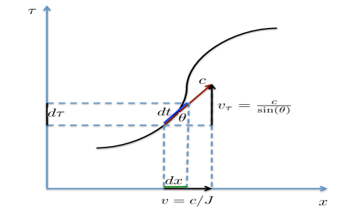
More generally, let $v$ be the norm of the configuration space velocity. $K$ is exactly the cosine of the angle between the normal to the surface spanned by trajectories in space-proper time and the line of sight to the space slice, $1/J=K=v/c$ .

If we set the observable phase $Y$ to satisfy, in any dimension

-\frac{\hbar D_{x}Y}{m}={\bf v},

(35)

where $D_{x}Y$ is the reduction of the differential $DY$ to the space slice of $M$ , then

\frac{\hbar|D_{x}Y|}{m}=v=\frac{c}{J},

(36)

where $v=|{\bf v}|$ , and $m$ is a constant²²2In classical optics, $J=c/v$ is the index of refraction. . Thus the velocity measures the spatial change in the phase of the observable. This corresponds to the non-relativistic case: while the relativistic action with no external potentials given by

S=\alpha\int\sqrt{-c^{2}\dot{t}^{2}+\dot{x}^{2}+\dot{y}^{2}+\dot{z}^{2}}

(37)

where $\alpha=imc$ , the classical action is

S_{c}=\frac{m}{2}\int[\dot{x}^{2}+\dot{y}^{2}+\dot{z}^{2}]dt

(38)

where $t$ is the classical time and $\tau=t$ .

Note that with identification

m=\frac{\rho\hbar}{c},

(39)

that has dimensions of mass (see Appendix A), we get

\frac{|DY_{x}|}{\rho}=\frac{1}{J}\Rightarrow|DY_{x}|=\frac{\rho}{J}

(40)

For the wavefunction, we have

\psi=\frac{\rho}{i|D_{x}Y|e^{iY}}=-iJe^{iY}.

(41)

We consider the flat $1+1$ space-time. As above, we assume that the wavefunction $\rho$ satisfies

\frac{\partial\rho}{\partial\tau}+v\frac{\partial\rho}{\partial x}=0.

(42)

i.e. $\rho$ is invariant on space-time trajectories. We let the observation field $f:{\mathbb{R}}^{2}\rightarrow{\mathbb{C}}$ be given by

f=e^{iY}

(43)

The “observable wavefunction” $\psi$ on the $x$ axis is defined by

\psi=\frac{\rho}{i|df/dx|}=\frac{\rho}{i|\frac{\partial Y}{\partial x}|e^{iY}}=\frac{\rho}{iKe^{iY}}.

(44)

We proceed to derive an equation of evolution for $\psi$ . We set

D_{\tau}Y=Y_{\tau}+vY_{x}={\tilde{\mathscr{L}}},

(45)

and obtain

\psi_{\tau}=-v\psi_{x}-v_{x}\psi-i{\tilde{\mathscr{L}}}\psi,

(46)

or, more compactly

i\hbar\frac{\partial\psi}{\partial\tau}={\mathscr{H}}\psi.

(47)

where

{\mathscr{H}}=(-i\hbar v\frac{\partial}{\partial x}+\hbar{\tilde{\mathscr{L}}})-i\hbar v_{x}.

(48)

The equation (47), extended to $d$ -dimensional configuration space reads

\psi_{\tau}=-{\bf v}\nabla\cdot\psi-\nabla\cdot{\bf v}\psi-i{\tilde{\mathscr{L}}}\psi,

(49)

and has the solution

\psi({\bf y},\tau)=\psi_{0}({\bf x}(X^{-\tau}({\bf y})))e^{-\int_{0}^{\tau}{\mathsf{div}{\bf v}({\bf x}(X^{-s}({\bf y})))}ds}e^{iS(\tau,{\bf y})/\hbar},

(50)

where $\psi({\bf z},0)=\psi_{0}({\bf z}),$ and $X^{-\tau}({\bf y})$ is the initial position at $\tau=0$ of trajectory landing at ${\bf y}$ at $\tau$ . In next sections we treat the non-relativistic case that makes use of these relationships.

Remark 4.

If we set $Y=-S/\hbar$ , the first term on the right side of (46) is just the quantization of the classical hamiltonian

H=vp+\hbar\tilde{\mathscr{L}}=vp-{\mathscr{L}},

(51)

where $p$ gets replaced by $-i\hbar\partial/\partial x$ and ${\mathscr{L}}=-\hbar\tilde{\mathscr{L}}$ is the lagrangian.

It is thus clear that in the current theory velocity and momentum are treated separately, like in the context of Dirac equation in Heisenberg representation [22], or Schwinger’s variational principle [23].

5.2 The Lagrangian

The relativistic lagrangian for a particle with no charge is usually stated as

{\mathscr{L}}_{0}=-\frac{mc^{2}}{\gamma}.

(52)

In [15] Fock developed the so-called proper-time formalism, that utilizes proper time as an independent variable and derived the relativistic Lagrangian for a particle with no charge as

{\mathscr{L}}=\frac{m}{2}||{\bf V}||^{2}-\frac{mc^{2}}{2}

(53)

Since then, the proper time formalism has proved useful in relativistic physics in a variety of contexts [24]. In the examples below, we utilize the Fock Lagrangian in equation (8). For the non-relativistic limit of the harmonic oscillator and particle-in-a-box, we utilize a recent formulation that relates the classical potential $U$ to the metric tensor component $g_{00}$ in mechanics on classical static curved spaces utilizing Gibbons formulation [25]:

ds^{2}=g_{00}c^{2}dt^{2}-|d{\bf x}|^{2}.

(54)

Let $U$ be a scalar potential source. As [26] shows, the condition $mv^{2}/2-U<<mc^{2}$ leads to

g_{00}\approx 1+\frac{2U}{mc^{2}}

(55)

{\mathscr{L}}_{c}\approx\frac{mv^{2}}{2}-\frac{mc^{2}}{2}g_{00}=\frac{mv^{2}}{2}-U-\frac{mc^{2}}{2}

(56)

It is interesting to note that the constant $mc^{2}/2$ stems from the time-component of the metric tensor. This is of consequence for the zero-point energy calculation in the examples that follow.

Example 1 (Free Particle).

Consider the free particle moving in flat $4$ -dimensional space-time with constant 4-velocity ${\bf V}$ . The divergence $\nabla\cdot{\bf V}=0$ . Recall that

t=\frac{\tau}{\sqrt{1-\nu^{2}/c^{2}}}=\tau\gamma,\ \gamma=1/\sqrt{1-\nu^{2}/c^{2}}.

(57)

Denote the space components of ${\bf V}$ by ${\bf U}$ . Since the velocity is constant, the lagrangian reads

{\mathscr{L}}=-mc^{2},

(58)

and thus from RQTE we get

i\hbar\gamma\frac{\partial\psi}{\partial t}+i\hbar{\bf U}\cdot\nabla\psi=mc^{2}\psi,

(59)

Let ${\bf u}={\bf U}/\gamma=(U_{1}/\gamma,U_{2}/\gamma,U_{3}/\gamma)$ . Then

i\hbar\gamma\frac{\partial\psi}{\partial t}+i\hbar\gamma{\bf u}\cdot\nabla\psi=-{{\mathscr{L}}}\psi.

(60)

5.3 Dispersion relationship

We next derive the dispersion relationship for the wave

\psi({\bf x},\tau)=Ae^{i({\bf k}\cdot{\bf x}-\omega t)}.

(61)

From (60) we get

\hbar\omega-\hbar{\bf k}\cdot{\bf u}=\frac{mc^{2}}{\gamma}=-{\mathscr{L}}_{0}.

(62)

Also, with $E=\hbar\omega$ and ${\bf p}={\bf k}\hbar$ we obtain

E=-{\mathscr{L}}_{0}+{\bf p}\cdot{\bf u}=mc^{2}\gamma,

(63)

and thus we get the correct relativistic expression for energy.

5.4 deBroglie relationships

We observe that one of our postulates is conservation of the wavenumber $\rho$ along the spacetime trajectory. Because of the discussion in Appendix B, leading to equation (103) we assume the natural frequency and wavenumber are related by

\omega=\rho c\gamma

(64)

which is just the “coordinate time” version of the relationship (102). The identification $m=\rho\hbar/c$ leads to

\hbar\omega=mc^{2}\gamma,

(65)

the first deBroglie wave-particle relationship. The dispersion equation (62) now yields

$\displaystyle mc^{2}\gamma-\hbar{\bf k}\cdot{\bf u}$	$\displaystyle=$	$\displaystyle\frac{mc^{2}}{\gamma},$
$\displaystyle mc^{2}-\frac{\hbar{\bf k}\cdot{\bf u}}{\gamma}$	$\displaystyle=$	$\displaystyle\frac{mc^{2}}{\gamma^{2}}=mc^{2}-m\bm{{\bf u}}\cdot{\bf u},$
$\displaystyle\frac{\hbar{\bf k}\cdot{\bf u}}{\gamma}$	$\displaystyle=$	$\displaystyle m\bm{{\bf u}}\cdot{\bf u},$	(66)

which in turn gives

{\bf u}=\frac{\hbar{\bf k}}{m\gamma},

(67)

which is the second deBroglie relationship as we set ${\bf p}={\bf u}m\gamma$ .

5.5 The relativistic wavepacket

The general solution to (60) reads

\psi({\bf x},t)=\psi_{0}({\bf x}-{\bf u}t)e^{-imc^{2}t/\hbar\gamma}

(68)

This solution is physical as long as $\int_{\mathbb{R}}|\psi_{0}|dx$ is finite and thus can be normalized to $1$ . For simplicity, we restrict to $1$ spatial dimension. Let

\psi_{0}(x)=Ae^{-x^{2}/2\sigma^{2}}=2\pi\sigma A\int_{\mathbb{R}}\phi(k)e^{ikx}dk

(69)

where

\phi(k)=e^{-\sigma^{2}k^{2}/2}.

(70)

By the second deBroglie relationship derived above, the velocity $u$ is

u=k\hbar/m\gamma

(71)

Integrating over the possible wavenumbers in a wavepacket, we get

$\displaystyle\psi(x,t)$	$\displaystyle=$	$\displaystyle 2\pi\sigma A\int_{\mathbb{R}}\phi(k)e^{ik(x-ut)}e^{-\frac{i}{\hbar}\frac{mc^{2}t}{\gamma}}dk$
	$\displaystyle=$	$\displaystyle 2\pi\sigma A\int_{\mathbb{R}}e^{(-\sigma^{2}k^{2}/2-it\frac{k^{2}\hbar}{m\gamma})}e^{-\frac{i}{\hbar}\frac{mc^{2}t}{\gamma}}e^{ikx}dk$
	$\displaystyle=$	$\displaystyle 2\pi\sigma A\int_{\mathbb{R}}e^{-k^{2}(\sigma^{2}/2+i\frac{t\hbar}{m\gamma})}e^{-\frac{i}{\hbar}\frac{mc^{2}t}{\gamma}}e^{ikx}dk.$
	$\displaystyle=$	$\displaystyle 2\pi\sigma A\int_{\mathbb{R}}e^{-k^{2}(\sigma^{2}+i\frac{2t\hbar}{m\gamma})/2}e^{-\frac{i}{\hbar}\frac{mc^{2}t}{\gamma}}e^{ikx}dk.$

For wavepacket of small width, where $\gamma(k)\approx const.$ , we get

\psi(x,t)=A\left(\frac{2\pi\sigma}{\sigma^{2}+i\frac{2t\hbar}{m\gamma}}\right)e^{\frac{-x^{2}}{\sigma^{2}+i\frac{2t\hbar}{m\gamma}}}e^{\frac{i}{\hbar}\frac{mc^{2}t}{\gamma}}

(73)

It is notable that the wavepacket width is suppressed (over the Schrödinger wavepacket derived below) due to the $t\hbar/m\gamma$ term. In fact, $\sigma^{2}+i\frac{2t\hbar}{m\gamma}\approx\sigma^{2}$ as $v\approx c$ . Such a suppression was observed in numerical simulations of electrons accelerated in intense laser fields [27, 28] using the Dirac equation considered on section 4.

Remark 5.

The solution (LABEL:trans1) can be interpreted in terms of energy as follows:

$\displaystyle\psi({\bf x},t)$	$\displaystyle=$	$\displaystyle A(2\pi\sigma)\int_{\mathbb{R}}\phi(k)e^{ik(x-ut)}e^{-\frac{i}{\hbar}\frac{mc^{2}t}{\gamma}}dk$
	$\displaystyle=$	$\displaystyle A(2\pi\sigma)\int_{\mathbb{R}}\phi(k)e^{ikx}e^{\frac{it}{\hbar}(-ku\hbar-\frac{mc^{2}}{\gamma})}dk$
	$\displaystyle=$	$\displaystyle A(2\pi\sigma)\int_{\mathbb{R}}\phi(k)e^{ikx}e^{-it\frac{E(k)}{\hbar}}dk$

And we see that the wavepacket is the combination of waves with positive energy. This is in contrast with the Dirac equation, where the combination of positive and negative energy states is used [29].

5.6 Non-relativistic dispersion relationship

The non-relativistic case is obtained by approximating the Lagrangian with

{\mathscr{L}}_{0}=-\frac{mc^{2}}{\gamma}+\frac{mu^{2}}{2}=-\frac{mc^{2}}{\gamma}+\frac{mk^{2}\hbar^{2}}{2m^{2}\gamma^{2}}=-\frac{mc^{2}}{\gamma}+\frac{k^{2}\hbar^{2}}{2m\gamma^{2}}

(75)

Setting $\gamma\approx 1$ , for a single particle in $1$ spatial dimension, we obtain

\psi(x,t)=\psi_{0}(x-ut)e^{i\frac{k^{2}\hbar t}{2m}}e^{-imc^{2}t/\hbar}

(76)

Integrating over the possible velocities in a $1+1$ wavepacket, we get

	$\displaystyle\psi(x-ut)$	$\displaystyle=$	$\displaystyle ae^{-imc^{2}t/\hbar}(2\pi\sigma)\int_{\mathbb{R}}e^{-k^{2}(\sigma^{2}+i2t\hbar/m)/2}e^{i\frac{k^{2}\hbar t}{2m}}e^{ik\cdot x}dk$
		$\displaystyle=$	$\displaystyle ae^{-imc^{2}t/\hbar}\left(\frac{\sigma^{2}}{\sigma^{2}+it\hbar/m}\right)^{1/2}e^{\frac{-x^{2}}{2(\sigma^{2}+it\hbar/m)}},$

which is also the result obtained from the Schrödinger equation.

The dispersion relationship is

$\displaystyle\hbar\omega-\hbar ku$	$\displaystyle=$	$\displaystyle mc^{2}-\frac{mu^{2}}{2}$
$\displaystyle\ \ \ \ \ \ \ \ \ \ \ \ E$	$\displaystyle=$	$\displaystyle\hbar\frac{k^{2}\hbar}{m}-\frac{mk^{2}\hbar^{2}}{2m^{2}}+mc^{2}$	(78)
	$\displaystyle=$	$\displaystyle\frac{k^{2}\hbar^{2}}{2m}+mc^{2}$	(78)

which, apart from the constant $mc^{2}$ term is the expression obtained from the Schrödinger equation.

Example 2.

We consider the example of the classical one-dimensional harmonic oscillator. The velocity field of the harmonic oscillator in classical space-time ( $\tau=t$ ) is given by (see figure 3)

	$\displaystyle\dot{x}$	$\displaystyle=$	$\displaystyle A\cos\omega t$
	$\displaystyle\dot{t}$	$\displaystyle\approx$	$\displaystyle 1.$		(79)

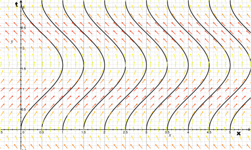
Thus, the divergence of the vector field is $0$ . The Lagrangian reads [26]

{\mathscr{L}}={\mathscr{L}}_{c}-\frac{1}{2}mc^{2}=\frac{1}{2}mv^{2}-\frac{1}{2}kx^{2}-\frac{1}{2}mc^{2}.

(80)

The trajectory of the harmonic oscillator in space time, taken for simplicity with the initial conditions $(x_{0},\dot{x}_{0}=0)$ satisfies

	$\displaystyle x(t)$	$\displaystyle=$	$\displaystyle x_{0}\cos\omega t$
	$\displaystyle\dot{x}(t)$	$\displaystyle=$	$\displaystyle x_{0}\omega\sin\omega t$		(81)

where $\omega^{2}=k/m$ . From (47), integrating over the period of the trajectory, we have

i\hbar\int_{\psi_{0}}^{\psi}\frac{d\psi}{\psi}=\int_{0}^{T}(\lambda+{\mathscr{L}})dt.

(82)

and thus

\psi(T)=\psi(0)e^{-\frac{i}{\hbar}\int_{0}^{T}(\lambda+{\mathscr{L}})dt}

(83)

In order for $\psi$ to be periodic, we have the condition

\int_{0}^{T}(\lambda+{\mathscr{L}})dt=n2\pi\hbar

(84)

where $n\in{\mathbb{Z}}$ . Now,

$\displaystyle\int_{0}^{T}{\mathscr{L}}_{c}dt$	$\displaystyle=$	$\displaystyle\int_{0}^{T}(\frac{1}{2}mv^{2}-\frac{1}{2}kx^{2})dt$	(85)
	$\displaystyle=$	$\displaystyle\int_{0}^{T}(\frac{1}{2}m(x_{0}\omega\sin\omega t)^{2}-\frac{1}{2}k(x_{0}\cos\omega t)^{2})dt$
	$\displaystyle=$	$\displaystyle\frac{x_{0}^{2}}{2}(m\omega^{2}-k)\int_{0}^{T}(\sin\omega t)^{2}dt$
	$\displaystyle=$	$\displaystyle 0,$

since

\int_{0}^{T}(\sin\omega t)^{2}dt=\int_{0}^{T}(\cos\omega t)^{2}dt,

(86)

and thus, from (84)

\lambda T-\frac{1}{2}mc^{2}T=n2\pi\hbar

(87)

From our previous consideration, using $m=\rho\hbar/c$ , we have

\frac{1}{2}mc^{2}T=\frac{1}{2}\rho\hbar cT=\frac{1}{2}\omega\hbar T

(88)

where $\omega=\rho c$ is deBroglie wave frequency. Finally, we get

\lambda=\frac{1}{2}\omega\hbar+n\hbar\omega=\omega\hbar(n+\frac{1}{2}).

(89)

which is exactly the standard result on the spectrum of the harmonic oscillator. The zero point energy $\omega\hbar/2$ arises from the oscillation of the observational field, since it comes from the lagrangian term.

Note that the nature of the spectrum is typical of weighted composition operators [30], and $n\hbar\omega$ is the spectrum of the underlying composition operator generated by setting ${\mathscr{L}}=0$ .

Example 3.

Consider the example of particle in a box of length ${l}$ . Since between impacts with the walls the particle has constant velocity $v$ , the classical limit of the Fock lagrangian (ommiting the constant $mc^{2}$ term) is [26]

{\mathscr{L}}=\frac{1}{2}mv^{2}

(90)

The particle moves with velocity $v$ between the walls. The eigenvalue problem reads

i\hbar v\frac{\partial\psi}{\partial x}=(\lambda-{\mathscr{L}})\psi

(91)

By integrating from $0$ to $l$

\frac{\lambda-{\mathscr{L}}}{\hbar}\frac{l}{v}=n\pi

(92)

i.e.

\lambda-{\mathscr{L}}=\hbar\frac{n\pi v}{l}

(93)

for $n\neq 0$ as $n=0$ leads to a trivial eigenfunction $0$ . De Broglie momentum relationship

p=mv=\frac{h}{\lambda_{p}}=\frac{2\pi\hbar}{\lambda_{p}}\Rightarrow v=\frac{2\pi\hbar}{m\lambda_{p}},

(94)

where $\lambda_{p}$ is the particle wavelength, leads to

{\mathscr{L}}=\frac{1}{2}mv^{2}=\frac{1}{2}m\frac{4\pi^{2}\hbar^{2}}{m^{2}\lambda_{p}^{2}}=\frac{2\pi^{2}\hbar^{2}}{m\lambda_{p}^{2}}

(95)

\lambda=\hbar^{2}\frac{n4\pi^{2}}{2ml\lambda_{p}}-L

(96)

Now we ask for “spatial” resonance, namely that the wavelength of string vibration is a subharmonic of the wavelength of the trajectory:

\lambda_{p}=\frac{2l}{n}

(97)

we get

L=\frac{\pi^{2}\hbar^{2}n^{2}}{2ml^{2}}

(98)

\lambda=\frac{\pi^{2}\hbar^{2}n^{2}}{ml^{2}}-L=\frac{\pi^{2}\hbar^{2}n^{2}}{2ml^{2}}.

(99)

Note that the relationship (97) indicates the nonlinearity of the dynamics: in the case of the harmonic oscillator treated in example 2, the frequency of oscillation of the trajectory was matched to the frequency of oscillation of the string. Here, the trajectory motion contains all of the harmonics of the base frequency, and the oscillation of the string can excite any of these.

6 Discussion and Conclusions

Starting from several postulates, in this paper we present a relativistic quantum transfer equation (RQTE) governing the evolution of a wavefunction transported by a 4-velocity field over a spacetime manifold. The key physical assumption is the existence of a complex scalar field (the horizontal lift) of the dynamics. When a probabilistic interpretation is sought, the solution of the equation reduces in the non-relativistic limit to the solution of the Schrödinger equation. In the special relativity limit, the equation is satisfied by the scalar part of the Dirac spinor. We obtained the classically known spectra from the RQTE formalism in the specific non-relativistic physical cases - the harmonic oscillator and the particle in the box. We additionally considered the problem of the Gaussian wavepacket. The solution of RQTE in this case yields a prediction that indicates reduction of wavepacket spreading in the limit when velocity approaches the speed of light in vacuum.

Solutions of QRTE lead to evolutions governed by specific type of transfer operators - the weighted composition operators. We believe this observation can be useful in further development of the theory and connections between the mathematical literature on such operators (see e.g. [20]).

It is of interest to note that from our postulates an interesting relationship between RQTE wavefunction and mass (or equivalently energy) emerges. In fact, the concept of mass that arises coincides with the concept of mass stemming from string theory considerations.

Extension of this theory for different spin particles is possible. We hope the developed theory might be useful in numerical methods needed for quantum computing problems.

Appendix A Mass and the Wavefunction

Recall,from our postulates, $\psi=(\rho/i|DY|)e^{-iY}$ . We note that $\psi$ , being a complex number, is nondimensional. For $\psi$ to be nondimensional, $\rho$ must have dimensions of a spatial wavenumber, [1/L] where $L$ is the unit of length.

Thus, one can think of the trajectories as carrying waves propagating in time with a certain frequency $\nu$ , where $\rho=\nu/c$ . Since $\rho\hbar/c$ has dimensions of mass, this is to indicate that spacetime trajectories oscillating at higher frequencies have higher “mass”. Vibrations theory teaches that higher frequencies of oscillation indicate higher stiffness, leading to the idea that mass reflects the “stiffness” of the underlying trajectory. Interestingly, this is in line with the concept of mass in string theory that is related to tension of the string [31, 32], see Appendix B.

Our postulates thus consistent with classical ideas on mass: 1) two objects with a different mass fall at the same speed, which is the consequence of our assumption that $\rho$ does not affect the velocity of objects in spacetime, and 2) it is harder to change the speed of an object (i.e. bend its trajectory in spacetime) if it has larger mass. In addition, the relationship $m=\rho\hbar/c$ introduces both $\hbar$ and $c$ into classical mechanics, since the classical momentum can be written as $p=\rho\hbar v/c$ , where $p$ is the linear momentum and $v$ is the velocity of the particle.

In fact, the definition of $Y=-S/\hbar$ is necessary precisely to offset the fact that in classical mechanics $m$ and not $\rho$ is used. The meaning of the constant $\hbar$ emerges as that of a conversion factor between the wavelength of oscillation of a particular space-proper time trajectory, and the associated, classically observable, mass. Mass, as defined here, is conceptually the rest mass of special relativity.

An analogy offers itself to lend physical intuition about the postulates: the situation is similar to that of observing objects moving at the bottom of a swimming pool through a wavefield on the surface. If the size of the object is much larger than the typical wavelength of the wavefield, their can be seen without an uncertainty proportional to that wavelength - small compared with the size of the object. However, if the object size is comparable to the wavelength, then the uncertainty in observation is large. In our case, the wavelength is $1/\rho=\hbar/mc$ , or precisely the reduced Compton wavelength.

Appendix B Relationship to String Theory

The ideas in this paper are consistent with deBroglie’s wave theory of matter, as we saw in section 5.4. But they are also supported by a mechanical model: the existence of the conserved wavenumber $\rho$ indicates that the nature of the underlying object is a string, traveling through space-time at speed $c$ . Consider the case of

S(\tau,{\bf y})=-mc^{2}\tau

(100)

arising from the relativistic lagrangian ${\mathscr{L}}=-mc^{2}$ (see the section 5.2 on the lagrangian). The frequency of oscillation of the observation field is

\Omega=\frac{mc^{2}}{\hbar}

(101)

Since the string has wavenumber $\rho$ , the associated natural frequency $\omega_{s}$ of oscillation of the string is

\omega_{s}=\rho c.

(102)

In the case of resonance

1=\frac{\omega_{s}}{\Omega}=\frac{\rho c\hbar}{mc^{2}},

(103)

which implies the wavenumber-mass relationship $m=\rho\hbar/c$ that we postulated based on dimensional grounds. This implies the existence of a matter object of mass $m$ provided there is a resonance between the internal frequency of oscillation of the string and the frequency of oscillation of the observation field.

Now we show that this analysis is consistent with the basic ideas in string theory. Consider an open string of length $\mathscr{l}_{s}$ [33]. Let the rest mass per unit length of the string be $\mu_{0}$ . Then the resonance condition reads

mc^{2}=\mu_{0}{\mathscr{l}}_{s}c^{2}=\rho\hbar c.

(104)

Let $T_{0}$ be the string tension. From [33], equation (7.26)

\sigma_{1}T_{0}=E=mc^{2},

(105)

we have

\sigma_{1}T_{0}=\rho\hbar c\Rightarrow T_{0}=\frac{\rho c\hbar}{\sigma_{1}}

(106)

Now we identify

\rho=\frac{1}{{\mathscr{l}}_{s}}.

(107)

This implies that conservation of $\rho$ on space-time trajectory is equal to the assumption of conservation of open string length. We get

T_{0}=\frac{\hbar c}{\sigma_{1}{\mathscr{l}}_{s}}

(108)

From (7.64) in [33] we have for the string rotational velocity $\omega_{s}$

\frac{\omega_{s}}{c}=\frac{\pi}{\sigma_{1}}\Rightarrow\sigma_{1}=\frac{\pi c}{\omega_{s}}=\frac{\pi{\mathscr{l}}_{s}}{2}

(109)

where the last part emerges from using $\omega_{s}{\mathscr{l}}_{s}/2=c$ from string theory (string ends have speed of light velocity if it has rotational velocity $\omega_{s}$ ), or alternatively by noting that

\omega_{s}=2\omega=2\rho c=\frac{2c}{{\mathscr{l}}_{s}}

(110)

from the current theory, since in string theory the frequency of repeat of string shape ${\mathbf{F}}$ for rotating string in spacetime is half the frequency (twice the period) based on string length. Thus,

T_{0}=\frac{2\hbar c}{\pi{\mathscr{l}}_{s}^{2}}

(111)

This is precisely what emerges from the formula (9.101) in [34].

An interesting aspect of this relationship is the nature of the energy term $mc^{2}$ - this is associated with the observable field oscillation, not with the string oscillation! In contrast, in string theory, the energy $E$ is the assumed property of the string.

References

[1] John Guckenheimer and Philip Holmes. Nonlinear oscillations, dynamical systems and bifurcations of vector fields. J. Appl. Mech, 51(4):947, 1984.
[2] B.O. Koopman. Hamiltonian systems and transformation in Hilbert space. Proceedings of the National Academy of Sciences of the United States of America, 17(5):315, 1931.
[3] Igor Mezić. Spectral properties of dynamical systems, model reduction and decompositions. Nonlinear Dynamics, 41(1-3):309–325, 2005.
[4] Marko Budisić, Ryan Mohr, and Igor Mezić. Applied koopmanism. Chaos: An Interdisciplinary Journal of Nonlinear Science, 22(4):047510, 2012.
[5] Frank Wilczek. Notes on Koopman-von Neumann mechanics and a step beyond. Unpublished, 2015.
[6] Ioannis Antoniou, Wladyslaw A Majewski, and Zdzislaw Suchanecki. Implementability of Liouville evolution, Koopman and Banach-Lamperti theorems in classical and quantum dynamics. Open systems & information dynamics, 9(4):301–313, 2002.
[7] E. Gozzi and D. Mauro. Minimal coupling in Koopman-von Neumann theory. Annals of Physics, 296(2):152–186, 2002.
[8] Partha Ghose. Continuous quantum-classical transitions and measurement: A relook. arXiv preprint arXiv:1705.09149, 2017.
[9] Ulf Klein. From Koopman-von Neumann theory to quantum theory. Quantum Studies: Mathematics and Foundations, 5(2):219–227, 2018.
[10] Denys I Bondar, François Gay-Balmaz, and Cesare Tronci. Koopman wavefunctions and classical–quantum correlation dynamics. Proceedings of the Royal Society A, 475(2229):20180879, 2019.
[11] David Viennot and Lucile Aubourg. Schrödinger–koopman quasienergy states of quantum systems driven by classical flow. Journal of Physics A: Mathematical and Theoretical, 51(33):335201, 2018.
[12] Ilon Joseph. Koopman-von Neumann approach to quantum simulation of nonlinear classical dynamics. arXiv preprint arXiv:2003.09980, 2020.
[13] Danilo Mauro. On Koopman–von Neumann waves. International Journal of Modern Physics A, 17(09):1301–1325, 2002.
[14] Dimitrios Giannakis. Quantum dynamics of the classical harmonic oscillator. arXiv preprint arXiv:1912.12334, 2019.
[15] V. Fock. Proper time in classical and quantum mechanics. Phys. Z. Sowjetunion, 12:404, 1937.
[16] Paul Adrien Maurice Dirac. General theory of relativity, volume 50. Princeton University Press, 1996.
[17] Peter J Olver. Applications of Lie groups to differential equations, volume 107. Springer Science & Business Media, 2000.
[18] Igor Mezić and Andrzej Banaszuk. Comparison of systems with complex behavior. Physica D: Nonlinear Phenomena, 197(1):101–133, 2004.
[19] Peter Holland. Computing the wavefunction from trajectories: particle and wave pictures in quantum mechanics and their relation. Annals of Physics, 315(2):505–531, 2005.
[20] RK Singh and JS Manhas. Composition operators on function spaces. Number 179. North Holland, 1993.
[21] James D Bjorken and Sidney D Drell. Relativistic quantum mechanics. McGraw-Hill, 1965.
[22] AO Barut and Nino Zanghi. Classical model of the dirac electron. Physical Review Letters, 52(23):2009, 1984.
[23] Kimball A Milton. Quantum Action Principle. Springer, 2015.
[24] J.R. Fanchi. Review of invariant time formulations of relativistic quantum theories. Foundations of physics, 23(3):487–548, 1993.
[25] G.W. Gibbons. The Jacobi metric for timelike geodesics in static spacetimes. Classical and Quantum Gravity, 33(2):025004, 2015.
[26] Sumanto Chanda and Partha Guha. Geometrical formulation of relativistic mechanics. International Journal of Geometric Methods in Modern Physics, 15(04):1850062, 2018.
[27] Alfred Maquet and Rainer Grobe. Atoms in strong laser fields: challenges in relativistic quantum mechanics. Journal of Modern Optics, 49(12):2001–2018, 2002.
[28] Qichang Su, BA Smetanko, and Rainer Grobe. Relativistic suppression of wave packet spreading. Optics Express, 2(7):277–281, 1998.
[29] Kerson Huang. On the zitterbewegung of the dirac electron. American Journal of Physics, 20(8):479–484, 1952.
[30] Gajath Gunatillake. Spectrum of a compact weighted composition operator. Proceedings of the American Mathematical Society, 135(2):461–467, 2007.
[31] David Tong. Lectures on string theory. arXiv preprint arXiv:0908.0333, 2009.
[32] Nick Huggett and Tiziana Vistarini. Deriving general relativity from string theory. Philosophy of Science, 82(5):1163–1174, 2015.
[33] Barton Zwiebach. A first course in string theory. Cambridge university press, 2004.
[34] Joel Franklin. Advanced mechanics and general relativity. Cambridge University Press, 2010.