A tale of two metrics:Polling and financial contributions as a measure of performance
Note: This paper has been accepted for publication in 2021 IEEE International Systems Conference (SysCon) proceedings ^††thanks:

Our study focused on two components: aggregated poll results and donation data collected from Federal Election Commision (FEC).

Different pollsters collect data with varying approaches such as phone calls and internet polls. They have distinct sampling sizes, sampling time, and potential biases in collecting the data. Appropriately aggregating the data from these polls helps to get a better estimation. The two well-known poll aggregators, FiveThirtyEight and RealClearPolitics, share aggregated values for the election. FiveThirtyEight also releases its rating for pollsters [7].

FiveThirtyEight collects poll data from different pollsters, rates them, finds their biases, and finally aggregates them to find the national average for different elections. The raw data, the rating, and biases of the pollsters are all available on FiveThirtyEight [8]. Fig. 1 from FiveThirtyEight shows the national average for each Democratic candidates in 2020 primary polls.

Fig. 1, shows the daily national average for each candidate but it is not easy to identify changes in the trend for each candidate nor see how significant events related to these changepoints. In the next section we use jointpoint regression to get more insight about this data.

We collected the donation data provided by the FEC official website [9]. The raw donation data contains information from multiple aspects of the donation and donor including date, donor’s name and zip-code. These information helps us distinguish the donors from each other, which provides a further possibility for counting and tracking each donor’s donation behavior towards multiple candidates.

Poll results represent estimated levels of support to each candidate on a given day. Donation data measures performance of each campaign independently and its comparison with polls requires data processing. Here we briefly discuss how we processed the raw data collected from official FEC wesite.

Based on the information of each donation and its donor, we processed the data for each candidate and obtained four metrics: the daily number of donors, daily number of new donors, daily donation amount from each donor, and daily donation amount from each donor.

The daily donor number is the total number of donors who have donated to a candidate on a specific day; the daily donation amount is the total amount of donation a candidate has received in a specific day. The daily number of new donors is the number of donors who donated to the candidate for the first time on that day. Note that a donor who has never donated to candidate A but has donated to candidate B in the past, will still be distinguished as a new donor of candidate A on the day of the donor’s first donation to candidate A no matter how many times the donor has donated to other candidates in the past; after the first donation to a specific candidate, a donor will not be distinguished as a new donor to this candidate. Correspondingly, the daily donation amount from new donors is defined as the total donation amount a candidate can receive from all the new donors on a specific day. These four metrics provide us the popularity and appeal of each candidate from the aspect of donation.

Moreover, we normalized the donation data by the total amount received over all candidates. This converts our measures into the daily proportion that went to each candidate. It is a two-step process: first, we find the sum of the total daily donations; second, the donations for each candidate are then divided by the sum of the total daily donations to represent the proportion.

A joinpoint regression model, also known as piecewise regression model or multi-phase regression, describes processes with multiple stages with variant trends. It can automatically detect the point that a change occurs as a “joinpoint”, hence differentiating the stages into multiple segments. Each segment is modeled as a linear function with fluctuations which manifests its trend. Joinpoints correspond to the changes in trend and bridge the stages together. Traditional trend modeling, including linear regression and time series, are often overly smooth for solving real-world problems, Joinpoint regression, however, is able to handle these conditions better in some aspects because of its ability to segment the time series. Joinpoint regression can provide insight of the time component and its relationship to variables of interest in a way that ordinary least squares and simple regression models may miss. By clearly identifying the point at which trends change, it highlights specific points in time that warrant further analysis and these models can be overlapped to allow for insight of whether one variable may lag or stimulate change in another.

Joinpoint regression models are frequently implemented in health sciences. Example studies include using joinpoint regression in predicting the trends of disease rates [10], mortality rates of diseases [11], and suicide rates [12]. Joinpoint regression has been used outside of health sciences as shown by its application to detect trends between food pantry use and long-term unemployment [13]. Joinpoint regression has also been applied to exploring relationships between disease rates and economic data to investigate the potential link or the existence of causality (economic variables affecting disease rates or vice versa) [14, 15], where the intervention of economic crisis or financial alterations have been detected as the interpretable factor contributing to the fluctuation of health-related problems.

Joinpoint regression is a tool for trend comparison. Identifying the similarity of trends in relevant variables can be used to provide insight of one variable as a potential predictor of another. The change points, the points that represent major changes in the trend, can be a tool to explore the causality of variables. The change points in the context of campaign performance can identify major events such as failure or success in a debate.

Identifying important events that resulted in changes in the trend is another application of change points. Change points that occur closely after an event may provide insights into the effect of the event on the overall trends for a candidate.

Joinpoint analysis can also reveal relationship insight from the data. By checking the timing of increased campaign donations and changes in poll position, it can give insights as to which variable leads the other and under what conditions. With domain knowledge of the data, it is also possible to explore and find answers to additional questions about the relationship between these variables. For example, can one be used to predict changes in the other? Does the relationship between polling and donations look the same at set milestones in the campaign or even across different candidates? And are there insightful trends in the data that can help distinguish the winning candidate from the others earlier on in the election process?

We applied joinpoint regression to the aggregated polling data sets. Fig. 2 is an illustration of joinpoint regression. In the joinpoint regression plots the green dots are the average percentage of the daily national polls. The black trend line represents the smoothed regression of the joinpoint analysis. The black vertical lines represent debate dates. The dashed vertical lines represent the major joinpoints for each metric. Blue lines indicate the start point for an increase in the trend slope and red lines indicate the start point of a decrease in the trend slope. These trends are further identified by the grey background which highlights when a trend is falling while the white regions represent a rising slope or trend.

Figure 2 uses data specific to 2020 presedential candidates Joe Biden, Bernard Sanders, Elizabeth Warren, and Pete Buttigieg starting May 15, 2019 and going to February 15, 2020. These four candidates were selected as they were the top candidates in the polls for Democratic primary polls.

We can use joinpoint analysis to identify and highlight event impacts for candidates. For example in Figure 2 we can observe that there is an alignment of trend shifts occurring in October. October 15, 2019 is when the fourth debate occurred and may be be the correlation of these aligned trend shifts. From the joinpoint plot it appears that Elizabeth Warren was impacted negatively by this event as her trend switched from a positive trend to negative. Pete Buttigieg an Bernard Sanders

• •

  Immediately after the fourth debate on October 15th, there are change points in the average polling result for Bernard Sanders, Elizabeth Warren, and Pete Buttigieg. Warren had experienced a great rising trend before this debate and she became one of the front-runners. Most of the other candidates attacked her she lost this debate. On the other hand, Pete Buttigieg and Bernard Sanders were among the winners of this debate [17].

• •

  For longer than a month Warren experienced a falling trend after the fourth debate but Bernard Sanders and Pete Buttigieg experienced a rising trend. It looks what Warren lost was a gain for the other two candidates.

• •

  Pete Buttigieg was one of the winners in the fifth debate[18] and we can observe its effect on the trends after the debate.

We applied joinpoint regression to both the aggregated polling and the donation data sets in Fig. 3. This figure uses data specific to the Bernard Sanders who was one of the top candidate in the polls at that time. The green dots are daily poll aggregations, new donations, new donors, total donors and total donation . The black line through them is the trend for a specific variable.

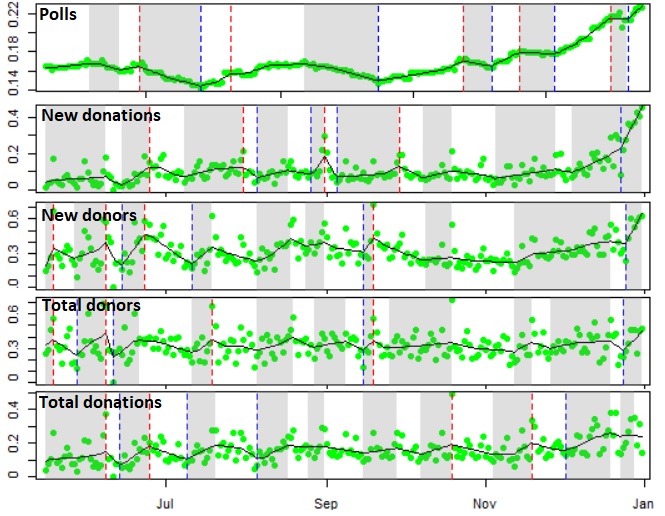
We can observe the followings in Fig. 3,

• •

  The falling and rising trends across different donation metrics are similar. This fact implies their dynamic is very similar.

• •

  Most of the times, a change point in the polling data occurs very close to a change point in at least one of the donation data.

• •

  Steep slopes in the polling data occurs when there are similar steep slopes in the donation data. As a result, steep slopes in one metric can indicate similar trend in the other.

These observation implies that polling and donation data are alternative measure of campaign performance. When there is uncertainty about the accuracy of one, the other improves the interpretation of that metric.

Fig. 4 similarly uses data specific to the candidate Joe Biden for the same period.

The change points can help identifying the events that caused change of the trends. For example, looking at poll results for Kamala Harris and Joe Biden in Fig. 5 we can find two close change points in late June and early July.

Checking the headlines from New York Times in that period shown in Fig. 6 we can find how her fight with Joe Biden in the first debate helped her to become more successful. On the other hand, in the same period of time, Joe Biden was less successful comparing to the trend before the debate.

So far we have focused on how these metrics compare across candidates. Another application of this analysis is finding the different dynamics across metrics for one candidate. In this case, we don’t need to normalize the data based on their daily summations. We can apply joinpoint regression on the raw data in this case. In Fig. 7, we can observe the result of joinpoint regression on the raw donation for Elizabeth Warren.

In the polling data shown in Fig. 7, Elizabeth Warren had a rising trend before mid-October and a falling trend afterward. Mid-October is the time of the fourth debate and most of the other candidates attacked her on the debate since she had became one of the front-runners.

If we look at the donation data in Fig. 7, all the metrics had a change point in early October. October 1st was the deadline for satisfying the fourth debate requirements. It is not surprising that her campaign asked her supporters to donate before this deadline. Other candidates had the same deadline and so if we normalized the donation data we expect the trends to be different. In Fig. 8 the normalized donation data is shown. As we can see, the change points are shifted to the right.

Comparing Fig. 8 and Fig. 7, we observe the blue change points occur after the fourth debate in the normalized donation data but not the raw data. It explains these change points are mainly resulted from increased support for other candidates which affects the denominator in the normalizing process.

References

- [1] L. M. Bartels, Presidential primaries and the dynamics of public choice. Princeton University Press, 1988.
- [2] A. R. Brown, “Does money buy votes? the case of self-financed gubernatorial candidates, 1998–2008,” Political Behavior, vol. 35, no. 1, pp. 21–41, 2013.
- [3] K. Lipsitz and C. Panagopoulos, “Filled coffers: Campaign contributions and contributors in the 2008 elections,” Journal of Political Marketing, vol. 10, no. 1-2, pp. 43–57, 2011.
- [4] G. C. Jacobson and J. L. Carson, The politics of congressional elections. Rowman & Littlefield, 2019.
- [5] A. Bonica, “Professional networks, early fundraising, and electoral success,” Election Law Journal, vol. 16, no. 1, pp. 153–171, 2017.
- [6] M. Koerth-Baker, “How money affects elections,” 2018.
- [7] N. Silver, “How fivethirtyeight calculates pollster ratings,” Internet, http://fivethirtyeight. com/features/how-fivethirtyeight-calculates-pollster-ratings/, accessed on February, vol. 2, p. 2015, 2014.
- [8] FiveThirthyEight. ”who’s ahead in the national polls?,” mar. 11, 2021. [Online]. Available: https://projects.fivethirtyeight.com/polls/president-primary-d/national
- [9] F. E. Commission, Federal Election Commission, 2020 (accessed August 01, 2020). [Online]. Available: https://www.fec.gov/
- [10] H.-J. Kim, M. P. Fay, E. J. Feuer, and D. N. Midthune, “Permutation tests for joinpoint regression with applications to cancer rates,” Statistics in medicine, vol. 19, no. 3, pp. 335–351, 2000.
- [11] E. Fernández, J. González, J. Borras, V. Moreno, V. Sánchez, and M. Peris, “Recent decline in cancer mortality in catalonia (spain). a joinpoint regression analysis,” European Journal of Cancer, vol. 37, no. 17, pp. 2222–2228, 2001.
- [12] H. Hedegaard, S. C. Curtin, and M. Warner, “Increase in suicide mortality in the united states, 1999–2018,” NCHS Data Brief, 2020.
- [13] G. Shackman, C. Yu, L. S. Edmunds, L. Clarke, and J. P. Sekhobo, “Relation between annual trends in food pantry use and long-term unemployment in new york state, 2002–2012,” American journal of public health, vol. 105, no. 3, pp. e63–e65, 2015.
- [14] C. C. Lubitz, C. Y. Kong, P. M. McMahon, G. H. Daniels, Y. Chen, K. P. Economopoulos, G. S. Gazelle, and M. C. Weinstein, “Annual financial impact of well-differentiated thyroid cancer care in the united states,” Cancer, vol. 120, no. 9, pp. 1345–1352, 2014.
- [15] E. Regidor, G. Barrio, M. J. Bravo, and L. de la Fuente, “Has health in spain been declining since the economic crisis?” J Epidemiol Community Health, vol. 68, no. 3, pp. 280–282, 2014.
- [16] T. B. Arnold, R. J. Tibshirani, M. T. Arnold, and T. ByteCompile, “Package ‘genlasso’,” Statistics, vol. 39, no. 3, pp. 1335–1371, 2020.
- [17] C. Cillizza, “Chris cillizza’s winners and losers from the fourth democratic debate,” CNN, Oct. 16, 2019. [Online]. [Online]. Available: https://www.cnn.com/2019/10/15/politics/who-won-the-democratic-debate/index.html
- [18] ——, “Chris cillizza’s winners and losers from the fifth democratic debate,” CNN, Nov. 21, 2019. [Online]. [Online]. Available: https://www.cnn.com/2019/11/20/politics/who-won-democratic-debate/index.html
- [19] J. Martin and K. Glueck, “Joe biden and kamala harris bring their debate-stage fight to iowa,” The New York Times, Jul. 4, 2019. [Online]. [Online]. Available: https://www.nytimes.com/2019/07/04/us/politics/joe-biden-kamala-harris-busing-iowa.html
- [20] M. S. McKinney and B. R. Warner, “Do presidential debates matter? examining a decade of campaign debate effects,” Argumentation and Advocacy, vol. 49, no. 4, pp. 238–258, 2013.