A Tale of Two Disks: Mapping the Milky Way with the Final Data Release of APOGEE
Abstract
We present new maps of the Milky Way disk showing the distribution of metallicity ([Fe/H]), -element abundances ([Mg/Fe]), and stellar age, using a sample of 66,496 red giant stars from the final data release (DR17) of the Apache Point Observatory Galactic Evolution Experiment (APOGEE) survey. We measure radial and vertical gradients, quantify the distribution functions for age and metallicity, and explore chemical clock relations across the Milky Way for the low- disk, high- disk, and total population independently. The low- disk exhibits a negative radial metallicity gradient of dex kpc-1, which flattens with distance from the midplane. The high- disk shows a flat radial gradient in metallicity and age across nearly all locations of the disk. The age and metallicity distribution functions shift from negatively skewed in the inner Galaxy to positively skewed at large radius. Significant bimodality in the [Mg/Fe]-[Fe/H] plane and in the [Mg/Fe]-age relation persist across the entire disk. The age estimates have typical uncertainties of in (age) and may be subject to additional systematic errors, which impose limitations on conclusions drawn from this sample. Nevertheless, these results act as critical constraints on galactic evolution models, constraining which physical processes played a dominant role in the formation of the Milky Way disk. We discuss how radial migration predicts many of the observed trends near the solar neighborhood and in the outer disk, but an additional more dramatic evolution history, such as the multi-infall model or a merger event, is needed to explain the chemical and age bimodality elsewhere in the Galaxy.
Accepted to ApJ July 21, 2023
1 Introduction
The positions, chemical compositions, and ages of individual stars in the Milky Way reflect the formation and evolution history of our Galaxy, with each individual star acting as a “fossil” containing the chemical fingerprint of the interstellar gas from which it formed. Our inside perspective in the Milky Way grants the ability to study it in greater detail than any other galaxy, placing strong observational constraints on formation models and simulations of disk galaxies. For this reason, constraining the chemical and dynamical properties of the stellar populations in the Milky Way disk remains a cornerstone of modern galactic astronomy.
Understanding the present-day chemical structure of our Galaxy has been increasingly successful with the advent of large spectroscopic stellar surveys like APOGEE (Majewski et al., 2017), Gaia (Gaia Collaboration et al., 2021), Gaia-ESO (Gilmore et al., 2022), LAMOST (Luo et al., 2015), GALAH (Buder et al., 2018), RAVE (Steinmetz et al., 2020), and SEGUE (e.g., Yanny et al., 2009). These surveys obtain precise kinematic and chemical information for a combined millions of stars across the Milky Way, with increasing sample sizes and more complete spatial coverage with every generation of survey. When paired with precise distances and positions from Gaia astrometry (Gaia Collaboration et al., 2018, 2021), these large surveys can access the evolution history of a large fraction of the Galactic disk. Even stellar ages, notoriously difficult to infer as they previously could not be directly measured for individual stars, are now readily available through the precise measurements of the masses for thousands of red giant stars available through asteroseismology (e.g., Pinsonneault et al., 2018; Miglio et al., 2021). These asteroseismic data sets are additionally used as training sets for machine learning techniques, expanding the stellar sample with age estimates to hundreds of thousands of stars (e.g., Ness et al., 2016; Leung & Bovy, 2018; Anders et al., 2018; Mackereth et al., 2019; Wu et al., 2019; Ciucă et al., 2021, Stone-Martinez et al. 2023).
Despite this wealth of data, the debate remains heated around which physical processes played the largest roles in shaping the Milky Way’s disk. The structural and chemical distribution of stars in the Milky Way has been well studied, leading to the discovery of two main stellar components, the “thin” and “thick” disk near the solar neighborhood (e.g., Yoshii, 1982; Gilmore & Reid, 1983). These components are distinct in their dynamic signature, with the thick disk characterized by kinematically hotter stellar orbits (larger vertical velocity dispersion), and a slower systemic rotational velocity than the thin disk (e.g., Soubiran et al., 2003; Jurić et al., 2008; Kordopatis et al., 2013; Robin et al., 2017). The thin disk is also generally accepted to be more radially extended, and as the name implies, has a smaller scale height than the thick disk (e.g., Bensby et al., 2011; Bovy et al., 2016; Mackereth et al., 2017; Lian et al., 2022a; Robin et al., 2022). The two disks also differ in their chemical fingerprints, with the thin disk generally containing younger metal-rich stars characterized by their lower -element111-elements are elements with an atomic number multiple of 4 (the mass of a Helium nucleus, an -particle), e.g., O, Mg, S, Ca abundances relative to the older, more metal-poor thick disk (e.g., Fuhrmann, 1998; Bensby et al., 2005; Reddy et al., 2006; Lee et al., 2011; Bovy et al., 2012b, 2016; Nidever et al., 2014; Kordopatis et al., 2015a; Hayden et al., 2015; Mackereth et al., 2017; Vincenzo et al., 2021a; Katz et al., 2021). The [Mg/Fe] ratio reflects the relative iron enrichment by prompt, massive core-collapse supernovae compared to the longer timescale Type Ia supernovae. Because of this, the [Mg/Fe] ratio is generally high in populations that formed during rapid and efficient starbursts, and approaches solar “-poor” values in populations that form steadily over long time periods (e.g., Matteucci & Brocato, 1990; Thomas et al., 2005). Thus, the chemical differences between the thin and thick disk suggests that they formed via distinct pathways, leaving the evidence of their enrichment histories within the present-day chemical structure of the Galaxy. However, many of these studies are biased towards the solar neighborhood due to observation limitations, and there has been some debate on whether the two components are truly distinct at all (e.g., Bensby et al., 2007; Bovy et al., 2012a; Kawata & Chiappini, 2016; Hayden et al., 2017; Anders et al., 2018).
Nevertheless, different explanations for the origins of this chemical bimodality in the disk have been proposed, using a combination of physical processes such as star formation, gas accretion, quenching, galaxy mergers, and stellar radial migration to attempt to explain the observed trends. The different models can be generally categorized into three scenarios: the “two-infall” models where the thick disk forms first followed by the thin disk, the “superposition” models where the two disks form in different parts of the Galaxy and mix through stellar migration, and the “clumpy formation” models where the two disks form simultaneously but with different star formation efficiencies.
The “two-infall” class of models, originally of Chiappini et al. (1997) and Chiappini et al. (2001), describe a scenario wherein the Milky Way first forms from the collapse of primordial gas, creating the progenitor of the present-day thick disk in a fast burst of star formation. The gas reservoir of the Galaxy is then quenched, entering a quiescent period of little star formation until the Galaxy receives a second infall of pristine gas. This accretion of fresh material dilutes the metallicity of the interstellar medium before reigniting star formation that forms the thin disk. The second gas infall happens over a longer time scale, allowing for a period of more continuous star formation, resulting in the -poor nature of thin disk. Linden et al. (2017) constrained the timing of the second infall to be between 7-8 Gyr ago based on the ages and chemistry of star clusters in APOGEE. Spitoni et al. (2019a, 2020, 2021) expand on this model, constraining the length of the delay between the two episodes of gas infall to be between 3 - 5.5 Gyr, and proposing the second gas infall corresponds to a merger event with a gas-rich dwarf galaxy around 8-11 Gyr ago. This may coincide with the Milky Way’s accretion of the Gaia-Enceladus dwarf galaxy, estimated to have happened 10 Gyr ago (Helmi et al., 2018; Vincenzo et al., 2019).
A number of three-infall models have also recently been proposed, including the model of Spitoni et al. (2022b) constrained to Gaia data. Their most recent infall starts 2.7 Gyr ago and gives birth to the recently discovered young, low- stars that are impoverished in some elements (Gaia Collaboration et al., 2022). This latest infall may be linked with the Sagittarius dwarf spheroidal galaxy’s most recent perigalactic passage through the Milky Way’s disk (Ruiz-Lara et al., 2020; Laporte et al., 2019; Antoja et al., 2020). A starburst 2-3 Gyr ago has been detected independently in Isern (2019) and Mor et al. (2019).
The works of Lian et al. (2020a, b, c) and Lian et al. (2021) present a modified version of the two-infall model. In their version, an underlying continuous episode of gas accretion is interrupted by two rapidly quenched starbursts. The first starburst forms the high- thick disk, and the second starburst forms the metal-poor end of the low- sequence 6 Gyr later. The metal-rich low- sequence is attributed to the secular evolution phase between the two bursts.
Another variation of the two-infall model without the inclusion of merger events has been supported by recent chemo-dynamical simulations from Khoperskov et al. (2021). As in previous models, the thick disk is formed early on in a burst of star formation in a turbulent, compact disk. Stellar feedback from the formation of the thick disk drives outflows that quench star formation, enrich the Galactic halo, and eventually, feed the gas back into the disk on a more sustained timescale, creating the thin disk with a “galactic fountain” (e.g., Shapiro & Field, 1976; Bregman, 1980; Marinacci et al., 2011; Fraternali, 2017). The models of Haywood et al. (2016, 2018, 2019) support this scenario, where the high- population was formed early on in a turbulent gas-rich disk with strong feedback, and the leftover, diluted gas forms the low- thin disk on longer timescales.
The “superposition” class of chemical evolution models, pioneered by Schönrich & Binney (2009a, b), reproduce the observed disk dichotomy without the need for a violent merger history to heat the thick disk. In this scenario, the chemical locus of the thin disk is not an evolutionary track; it is a superposition of end points of evolutionary tracks from different Galactocentric radii (e.g., Nidever et al., 2014; Kubryk et al., 2015; Sharma et al., 2021a). Stars from these different tracks reach the solar neighborhood by radial migration, a natural consequence of the Galaxy’s spiral structure (Sellwood & Binney, 2002; Roškar et al., 2008). Stars in the high- thick disk formed early during an efficient phase of rapid star formation, primarily in the inner Galaxy, before migrating to their present day radial distribution.
This superposition model is expanded on in the works of Minchev et al. (2013, 2014), Minchev et al. (2017), and Johnson et al. (2021), which also emphasize the importance of radial migration in the Milky Way’s structure. In these models, gas inflows, outflows, and star formation rates vary with Galactic location, emphasizing the radial dependence of the disk’s chemical evolution history. Stellar radial migration allows stars to move around the Galaxy as time progresses, and potentially enrich a different spatial zone than the one they were born in when they die. These models show that this radial migration is the key to reproducing many of the observed trends in the Milky Way, including the changes of [Mg/Fe] and [Fe/H] distributions with radius and height.
A third, qualitatively different scenario is proposed by the “clumpy formation” model of Clarke et al. (2019), motivated by results from hydrodynamical simulations (e.g., Bournaud et al., 2007) and observations of high-redshift galaxies (e.g., Elmegreen et al., 2005). In their picture, the low- thin disk is a true evolutionary sequence corresponding to inefficient star formation in the disk, while the high- population is formed mainly during rapid, clumpy bursts in the Galaxy’s early gas rich phase. These clumps are comparable to those observed in high-redshift galaxies with the Hubble Space Telescope (e.g., Elmegreen et al., 2005). In addition to the chemical bimodality, these models also reproduce the observed mass density structure of the Milky way, including the flared thin disk (Beraldo e Silva et al., 2020; Amarante et al., 2020).
The discrepancy between these different proposed explanations, which all reasonably reproduce the observed trends in the Milky Way’s disk, can only be closed with more observational constraints. Detailed chemical maps that cover the entire span of the disk, robust measurements of the Milky Way’s radial and vertical metallicity gradients, and the metallicity distribution function will help constrain which physical processes played an important role in the formation of the disk. Adding in the ages of stars can provide an important axis for interpreting these results, as they enable a direct temporal connection between the properties of individual stars and the evolutionary time scale of the Milky Way (e.g., Mackereth et al., 2017; Feuillet et al., 2019; Vázquez et al., 2022).
In this paper, the final data release of the Apache Point Galactic Evolution Experiment (APOGEE; Majewski et al., 2017; Abdurro’uf et al., 2022) is used to further explore the properties of the Milky Way, with a larger sample size and greater spatial coverage than previously available.
The chemical cartography of the Milky Way has been extensively studied previously using a variety of different surveys including SEGUE (e.g., Lee et al., 2011, 2011; Gómez et al., 2012), RAVE (e.g, Kordopatis et al., 2013; Robin et al., 2017), GALAH (e.g., Lin et al., 2019; Hayden et al., 2020; Sharma et al., 2021b), LAMOST (e.g., Huang et al., 2020; Vickers et al., 2021; Hawkins, 2022), Gaia (e.g., Lemasle et al., 2018; Gaia Collaboration et al., 2022; Poggio et al., 2022), Gaia-ESO (e.g., Bergemann et al., 2014; Kordopatis et al., 2015a; Magrini et al., 2018; Vázquez et al., 2022), and previous data releases of APOGEE (e.g., Nidever et al., 2014; Hayden et al., 2015; Weinberg et al., 2019; Eilers et al., 2021; Katz et al., 2021). These works, and others, have impressively advanced the field of chemical cartography over the last decade, meaning that many of the results presented in this paper are not new. However, the final data release of APOGEE presents a larger and more detailed base data set than previously available. This allows us to cull a selected high-quality sample, minimizing systematics while still probing a large number of stars at different locations across the Galaxy. Additionally, APOGEE has the distinct advantage of working in the infrared, easily accessing the heavily dust-obscured regions like the Galactic center and mid-plane, which are often beyond the reach of optical surveys.
Our study complements the DR17-based study of Weinberg et al. (2022), which focused on abundance trends of [X/Mg] for many different elements. These trends, which are nearly universal throughout the disk, provide insights on nucleosynthetic processes, while the distribution of stars in [Mg/Fe], [Fe/H], and age across the disk provide constraints on Galactic history.
In this work, we build upon the decades of previous discoveries and explore the chemical trends in the Milky Way disk through the legacy of the APOGEE survey. A high-quality sample of red giant stars and their precise measurements of metallicity ([Fe/H]), ages, and -element abundances ([Mg/Fe]) are used to create maps, measure gradients, quantify distribution functions, and trace age-abundance relations across the Milky Way disk, and compare the observations with the most recent models. In short, we find evidence supporting all three classes of chemical evolution models; Radial migration is an important process in shaping the disk over time, but the observed bimodality in -element abundances and ages persists even in disk regions where radial migration is not expected to be as prevalent. This suggests a multi-phase star formation history, such as that presented in the two-infall or clumpy formation class of models, is at least partially responsible for the formation of the Milky Way as seen today.
Section 2 contains an overview of the APOGEE survey and supplementary data used in this study. Spatial maps, gradient measurements, distribution functions, and other results are presented in Section 3 and compared with previous literature. In Section 4, we discuss our results in the context of chemical evolution models. The conclusions we draw from this study are presented in Section 5.
2 Data
2.1 APOGEE
The Apache Point Observatory Galactic Evolution Experiment (APOGEE; Majewski et al., 2017) is a high-resolution () near-infrared ( m) spectroscopic survey containing observations of 657,135 unique stars released as part of the SDSS-IV survey (Blanton et al., 2017). The spectra were obtained using the APOGEE spectrograph (Wilson et al., 2019) mounted on the m SDSS telescope (Gunn et al., 2006) at Apache Point Observatory to observe the Northern Hemisphere (APOGEE-N), and expanded to include a second APOGEE spectrograph on the m Irénée du Pont telescope (Bowen & Vaughan, 1973) at Las Campanas Observatory to observe the Southern Hemisphere (APOGEE-S). The final version of the APOGEE catalog was published in December 2021 as part of the 17th data release of the Sloan Digital Sky Survey (DR17; Abdurro’uf et al., 2022) and is available publicly online through the SDSS Science Archive Server and Catalog Archive Server222Data Access Instructions: https://www.sdss.org/dr17/irspec/spectro_data/.
The APOGEE data reduction pipeline is described in Nidever et al. (2015). Stellar parameters and chemical abundances in APOGEE were derived within the APOGEE Stellar Parameters and Chemical Abundances Pipeline (ASPCAP; Holtzman et al., 2015; García Pérez et al., 2016; Holtzman et al., 2018; Jönsson et al., 2020, J.A. Holtzman et al. 2022 in prep.). ASPCAP derives stellar atmospheric parameters, radial velocities, and as many as 20 individual elemental abundances for each APOGEE spectrum by comparing each to a multi-dimensional grid of theoretical model spectra (Mészáros et al., 2012; Zamora et al., 2015) and corresponding line lists (Shetrone et al., 2015; Smith et al., 2021), employing a minimization routine with the code FERRE (Allende Prieto et al., 2006) to derive the best-fit parameters for each spectrum. We highlight that several elements (notably [Mg/Fe]) were updated in DR17 to include non-LTE effects in the stellar atmosphere. ASPCAP reports typical accuracy in metallicity measurements within 0.01 dex (Jönsson et al., 2018). In this study, we adopt the calibrated values for surface gravity (), metallicity ([Fe/H]), and -element abundances ([Mg/Fe]) from ASPCAP. We adopt [Mg/Fe] for our -element abundance instead of the “total” [/M], because [Mg/Fe] is the most precisely measured abundance by ASPCAP, and this element ratio has been traditionally used to define the boundary between the chemical thin and thick disk.
2.2 Sample Selection


Several cuts were made to the full APOGEE catalog to refine our sample. First, only stars defined as APOGEE main survey targets (also sometimes called the “main red giant sample”) were selected using the EXTRATARG flag. This removes any duplicate entries, as well as any ancillary science or other survey stars that were targeted for observation for a specific purpose (e.g., satellite or dwarf galaxy targets, star cluster member candidates, Kepler Objects of Interest). The main survey targets were randomly selected for observation from the 2MASS catalog, based on their color and -band apparent magnitude. For more information on the targeting strategies of APOGEE, see Zasowski et al. (2013, 2017), Beaton et al. (2021), and Santana et al. (2021).
Stars with noisy spectra () or unreliable parameter estimates from ASPCAP were removed from our sample using the SN_BAD and STAR_BAD ASPCAP bits respectively. The latter is triggered when the derived parameters for a star are designated a bad fit by its high value, when the derived temperature does not match the star’s observed color, when any individual stellar parameter measurement is flagged as bad, or when the derived parameters lie on an edge of the synthetic spectral grid.
The sample is further restricted to stars with surface gravity values between . Limiting to a small range in minimizes potential systematic uncertainties in abundance measurements, which tend to present as a function across Teff and in APOGEE (e.g., Jönsson et al., 2018; Eilers et al., 2021). The higher luminosity of these giants helps probe larger distances, allowing for a wide range of positions to be sampled across the Galactic disk in our study. Fainter stars may be better sampled closer to the Sun, but to keep our sample consistent across all distances, we apply this cut to ensure the trends we are documenting are not attributed to any systematic bias. Eilers et al. (2021) presents an empirical correction for these systematics for those interested; this would mainly be a concern if the expected distribution of in observations varies significantly with distance, which we do not expect in our sample. The lower limit is also imposed by the availability of asteroseismic data, as no age estimates are available for stars with in distmass.
Figure 1 shows the Teff- distribution of the sample after these refinements. The final number of stars in our RGB sample is 66,496. Due to the particulars of APOGEE field selection, there are more stars above the disk ( 38,031) than below ( 28,465), and more observations towards the Galactic center ( 36,317) than outward ( 30,179). The spatial distribution of our sample is shown in Figure 2. The stellar distance estimates used for this Figure (and the remaining of the paper) are described in Section 2.4.
In this work, we make no correction for the selection biases within the APOGEE survey. Stars close to the solar neighborhood will be over-represented in our sample. As shown in Figure 2, as distance from the Sun increases, the number of stars available in the APOGEE sample decreases.333This explanation is an oversimplification of the APOGEE selection function. The actual selection function depends on more than just distance from the Sun, as targeting strategies may vary between fields, observing time availability and instrument specifications differed between the North and South, and the non-homogeneous dust distribution in the Milky Way plays a major role in what can be observed. There are certain limitations that this selection function imposes on this work and similar studies. Specifically, results should not be averaged over a large spatial range, as the relative number of observed stars will clearly weight the average towards the solar neighborhood. Additionally, nothing can be inferred from the relative number of stars between locations, or about the intrinsic density profile of stars in the disk, because the former is heavily influenced by the selection function. That said, the effect of the selection function should be negligible when confined within a small spatial zone and limit in the Galaxy, such that general abundance trends and normalized number distributions should be consistent even without correcting for the APOGEE selection function (e.g., Hayden et al., 2015, Appendix A). In this work, we consistently bin stars in different ranges of and to avoid this bias and explore how chemical and age trends vary across the disk. A more complete prescription on how to account for the effects of the selection function in APOGEE has been published in Bovy et al. (2012b, 2016), Mackereth et al. (2017) for previous data releases, and Imig et al. (in prep.) for DR17. Imig et al. (in prep.) will present the density distribution of mono-age mono-abundance stellar populations in APOGEE DR17 after correcting for the selection function.
2.3 [Mg/Fe] Subsamples

Figure 3 shows the [Mg/Fe]-[Fe/H] plane for our full sample, where the bimodal distribution in [Mg/Fe] is obvious (e.g., Fuhrmann, 1998; Bensby et al., 2005; Reddy et al., 2006; Lee et al., 2011; Kordopatis et al., 2015a; Hayden et al., 2015; Katz et al., 2021). Although there is some debate on whether the two sequences are truly distinct (see Introduction), we use this figure to define two further subsamples in our data to investigate this question later. Vincenzo et al. (2021a) demonstrate that the distribution in [Mg/Fe] at fixed [Fe/H] is genuinely bimodal when considering the full disk population at near-solar radii, after accounting for the APOGEE selection function. We define the -poor “thin disk” sequence and the -rich “thick disk” sequence by splitting the full sample into two groups defined by a line in [Mg/Fe]-[Fe/H] space, shown in Figure 3. We adopt a similar limit as Weinberg et al. (2019, 2022) parameterized by the equation:
| (1) |
Our equation differs from Weinberg et al. (2019, 2022) by a small offset of [Mg/Fe] dex, correcting for abundance calibrations.
This separation in -element abundances is shown in Figure 3. A conservative buffer zone within dex of the line is excluded to remove potential overlap between the two sequences. This value is larger than the typical uncertainties of APOGEE abundance measurements, shown as the in the error bars across the bottom of the plot.
2.4 Age and Distance Estimates
Accurately mapping the Milky Way in three dimensions requires knowing precise distances to every star in our sample. Galactocentric positions were calculated for each star using the right ascension (RA) and declination (DEC) from APOGEE observations and distance estimates from the APOGEE distmass value added catalog (A. Stone-Martinez et al. 2023, submitted). The distmass distances were obtained through a neural network that was trained to estimate a star’s luminosity based on its ASPCAP parameters, using Gaia and cluster distances to provide the training labels. Distance estimates from the distmass catalog are typically precise within 10%. For the purpose of calculating Galactocentric coordinates, we define the reference location of the Sun to be kpc with a height of kpc above the plane (Bland-Hawthorn & Gerhard, 2016).
For evolved red giant stars, carbon and nitrogen abundances provide mass information because of the mass-dependence of stellar mixing (e.g., Iben, 1965; Salaris & Cassisi, 2005), allowing the determination of stellar masses for stars without asteroseismology (e.g., Martig et al., 2016; Vincenzo et al., 2021b). This fundamental property is used to derive stellar age estimates in the distmass catalog, wherein ages are derived by training a second neural network on the ASPCAP parameters of stars with asteroseismology masses from the APOGEE-Kepler overlap survey (APOKASC; Pinsonneault et al., 2018, APOKASC3: Pinsonneault et al. 2023 in prep.). The neural network learns the relations between the ASPCAP parameters and asteroseismic masses for stars from APOKASC, then it predicts the masses for all giant stars from DR17. Knowing the masses for evolved stars, ages can be derived through stellar evolution theory which predicts a star’s location on an isochrone. For the distmass catalog, isochrones from Choi et al. (2016) were adopted to make this conversion from derived mass to stellar age. The isochrones cover a range of ages (), metallicities (), and masses ().

The reported uncertainties on the age estimates in distmass are shown as a histogram in Figure 4 for our sample; the median lower uncertainty is (age) and the median upper uncertainty is (age). The uncertainties in stellar age are propagated from the uncertainties in stellar mass, which are predicted from the spread in mass from the neural network training set. The mass and age uncertainties have no strong dependence on metallicity or (A. Stone-Martinez et al. 2023, submitted).
To determine if these uncertainties are realistic, A. Stone-Martinez et al. (2023, submitted) performs an additional evaluation of the age estimates by comparing to previous literature. Compared to a small sample of cluster members with independent age estimates from main sequence turnoff fitting, they find that the distmass ages are accurate within in (age) across 12 different star clusters with ages (age) Gyr. Compared to a larger sample of field stars from the astroNN catalog (Leung & Bovy, 2018; Mackereth et al., 2019), the distmass ages show a typical spread of in (age), although these ages are derived with a similar methodology. Both of these evaluations are consistent within the reported age uncertainties.
Precise stellar ages remain difficult to measure robustly for large samples of stars. Neural network derived ages like distmass are heavily dependent on their training set values, and any uncertainties in the training set labels will influence the neural network model. The distmass catalog trains on stellar masses derived from asteroseismology, which have their own systematics and different groups have derived different results. Appendix A tests some of our results using different training sets and age catalogs, and motivates our choice of adopted ages. Even within distmass, there are six provided stellar age estimates for every star from neural networks trained on different asteroseismic mass estimates from three different research groups in APOKASC 3 (Pinsonneault et al. 2023 in prep.), and a set of “corrected” and “uncorrected” masses for each. The corrections are motivated by Gaia data, using parallaxes to calibrate the stellar radius derived from asteroseismology (e.g., Zinn et al., 2019). These corrections may be less reliable at lower and produce results that are less consistent across different bins in . For the remainder of this paper, we use the distmass results trained on the uncorrected SS ages from APOKASC 3 (Pinsonneault et al. 2023 in prep.), corresponding to the column named “AGE_UNCOR_SS” in the distmass catalog.
Selecting different age catalogs does make some difference in our results, particularly among the oldest stars as shown in Appendix A. Because this quantitative aspect can change considerably, we caution the reader against drawing strong conclusions from any of our age-related results without thoroughly understanding the related caveats outlined in Appendix A.
An additional quality flag from the distmass catalog is used to refine the sample when using the stellar age estimates. Namely, we remove stars that have bit 2 set, indicating stellar parameters Teff, [Fe/H], and lie outside of the range covered by the APOKASC training set; this removes stars with potentially unreliable mass (and therefore age) estimates. For anything involving ages, the full RGB sample is additionally restricted to 57,756 stars with this cut. Notably, all stars with [Fe/H] are excluded by this criterion. Metal-poor stars have extra mixing that was not learned by the neural network because there were no metal poor stars in the training set. Because metal-poor stars tend to be older, this means that for age related figures, the oldest stars ( years) may not be well-represented in our sample, particularly at large radii in the Galaxy; the potential effects of this, and other age-related caveats, are explored more in Appendix A.

3 Results
3.1 Cartography
Maps of the Galactic disk as a function of [Fe/H], [Mg/Fe], and stellar age are shown in Figure 5 in face-on ( plane; top row) and edge-on ( plane; bottom row) perspectives. The median value of each parameter is calculated for different spatial bins sized kpc, and shown as the respective color on the figure. For the edge-on perspective, the sign of the coordinate is applied to the coordinate, to better highlight the spatial coverage of the observations on the opposite side of the Galaxy.
In median metallicity (left column), clear radial and vertical metallicity gradients are visible in the disk, with higher average metallicities near the Galactic center that decline towards outer radii. In median -element abundances (middle column), the bimodality in the disk shows low- stars congregating in the “thin disk” near the Galactic midplane, and high- stars populating the “thick disk” at higher locations. At larger radii, the low- stars extend farther above and below the plane. The high- stars are more centrally concentrated. The right column, colored by median stellar age, contains fewer stars due to the additional cuts described in Section 2.4 when dealing with ages from the distmass catalog. Once again, radial and vertical gradients appear in these maps, as well as younger stars extending farther above the plane in the outer Galaxy. The innermost structural features of the Galaxy, such as the bar (noted by the ellipse) and bulge stand out as metal-rich, -poor, and older-aged than stars at similar radii but different azimuthal angles, consistent with previous studies of the central regions of the Galaxy (Wegg et al., 2019; Zasowski et al., 2019; Hasselquist et al., 2020; Eilers et al., 2021; Lian et al., 2021; Queiroz et al., 2021) for this metallicity range.


Dividing the maps into vertical bins reveals more nuanced structure; Figure 6 depicts face-on metallicity maps divided by height above the Galactic plane, from closest to the Galactic plane (top panel; kpc) to farthest away (bottom panel; kpc). The metallicity gradient is strongest close to the Galactic plane, with locations near the Galactic center showing a higher median metallicity than those at larger radii, as expected. Farther above the mid plane, the trend becomes less apparent, with almost no obvious gradient present when kpc, and the stellar populations showing a lower median metallicity overall. The middle panel ( kpc) shows a peculiar trend where the median metallicity actually increases from until kpc, and then decreases with a shallow metallicity gradient. This build-up of metal-rich stars in the center of the Galaxy is possibly the signature of the bulge.
The age distribution of the Galactic disk is shown in Figure 7. Again, the age gradient is strong close to the Galactic plane, with older stars more common near the center and younger stars dominating in the outer Galaxy. Unlike in metallicity, there is still a radial age gradient above the Galactic plane ( kpc), although in general the stars found above the plane are older than the stars found in the plane.
3.2 [Mg/Fe] Distribution


Figure 8 shows the Galactic distribution of stars in the [Mg/Fe]-[Fe/H] chemistry plane as a function of Galactic position. The different rows are the same vertical bins adopted in previous sections, with the bottom row closest to the Galactic plane ( kpc) and the top row farthest from the plane ( kpc). The columns are different radial bins, from closest to the disk center (left column) to farthest out (right column). Each panel shows the [Mg/Fe]-[Fe/H] distribution of stars in its respective spatial zone, colored by stellar point density (in Figure 8) and stellar age (in Figure 9). Our adopted definition of the split between the high- and low- sequences (equation 1) is plotted in black. For reference, the gray background highlights the distribution of the full sample, indicating the contour within which 90% of the sample is found.
Generally, the low- sequence is concentrated close to the Galactic plane (bottom row), and the high- sequence is more prominent outside the plane (top row) for kpc. The location of the high- sequence does not change based on location in the Galaxy. The low- sequence is more metal rich near the center of the Galaxy (left column), and moves to more metal-poor with increasing radius (right column). Additionally, at large radii, the low- sequence extends farther above the plane than it does close to the Galactic center. All of this has been well-documented in previous studies (e.g., Bensby et al., 2005, 2011; Nidever et al., 2014; Kordopatis et al., 2015a; Hayden et al., 2015; Katz et al., 2021; Vincenzo et al., 2021a; Gaia Collaboration et al., 2022).
Figure 9 shows the spatial distribution of [Mg/Fe] coded by stellar age. The high- sequence is composed of older stars at all radial bins. The low- sequence includes older stars close to the Galactic center ( kpc) and younger stars farther out in radius. At any radius, the lower [Mg/Fe] stars within the low- sequence have younger ages. Within the low- sequence, stellar age correlates more with [Mg/Fe] than it does with [Fe/H], indicating that the low- sequence is likely not a true single sequence.
To aid in the direct comparison between the radial and height bins, Figure 10 shows the contours (top panel) and median (bottom panel) in the [Mg/Fe]-[Fe/H] plane for both the low- and high- samples as a function of Galactic radius. In this Figure, the data are restricted to the plane ( kpc), equivalent to the bottom row in Figures 8 and 9. The contour containing 90% of points in both the low- and high- samples is shown in the top panel. The low- sequence is more metal-rich near the center of the Galaxy, and shifts continuously to lower metallicities and higher- moving outwards in radius. The high- sequence’s contour is generally the same shape and position at all radii, although close to the center of the Galaxy, the shape extends further to the metal-poor end. In the bottom panel, the median [Mg/Fe] as a function of metallicity is shown for both samples. As before, the low- sample shifts more metal-poor with increasing radius. The high- sequence moves slightly downwards (towards more -poor) with increasing radius. This is also seen in Katz et al. (2021) with APOGEE data, using the mode of the data, although they find a larger shift of dex between the inner and outer Galaxy, while ours is closer to half that at dex.

3.3 Azimuthal Variance in Metallicity
The degree to which trends in the Galactic disk are azimuthally symmetric has the potential to provide interesting insight into the history of the disk. The stellar distribution across the Galaxy is not uniform, with in-situ non-axisymmetric features such as the Galactic bar and spiral arms containing higher stellar density than surrounding populations, particularly for young stars (e.g., Bland-Hawthorn & Gerhard, 2016; Reid et al., 2019; Khoperskov et al., 2020a). Additionally, chemical enrichment is strongly dependent on local conditions, and spiral density fluctuations can lead to measurable differences in a galaxy’s enrichment history across azimuth (Spitoni et al., 2019b).
To look more closely at the azimuthal symmetry of the disk, the right column of Figure 11 is a metallicity map of the disk identical to Figure 6 but displayed in polar coordinates. The spatial bins are sized kpc and . As before, the stars are separated into rows based on their height above the Galactic plane. The corresponding panels to the left trace the median metallicity at each radius (y-axis) for different bins in azimuthal angle (point color), restricted to deg, where there is reasonable coverage with radius. At each radius, the expected spread based on uncertainty of the median measurements is shown as the gray shaded region. The expected spread () is defined for a given radius as the sum of the uncertainty in the median for each individual bin (), divided by the number of bins with valid data (), whereas the uncertainty in the median for a given azimuth bin is the standard deviation in [Fe/H] divided by the square root of the number of stars in that bin:
| (2) |
| (3) |
Close to the Galactic plane ( kpc, top row), the Galaxy has little metallicity variation across azimuth near the Solar neighborhood and outward ( kpc), although the region of azimuth covered by the observations decreases with increasing radius. Closer to the center of the Galaxy () kpc, the median metallicity varies more with azimuthal angle , with the spread possibly slightly exceeding the expected uncertainty. In the middle row higher above the Galactic plane ( kpc), a similar trend is seen, where there is more spread with metallicity in azimuth near the center of the Galaxy. There does seem to be an asymmetry in the disk that follows the approximate location of the Galactic bar in these coordinates, with metal-rich stars preferentially residing in the Galactic bar. Higher above the Galactic plane ( kpc, bottom row), the variation in azimuth can be attributed entirely to noise from low-number statistics, where the observed spread is all comparable or smaller than the expected spread.
Interactions with satellite galaxies and merger events can also perturb the disk in non-axisymmetric ways, such as warping the disk or introducing kinematic oscillations (e.g., Gómez et al., 2012; Cheng et al., 2020; Chrobáková et al., 2022). The restorative force from these perturbations is weaker in the outer Galaxy, so the presence of these features is generally expected to be more obvious at large radii. We find no significant azimuthal asymmetries in metallicity in the outer disk, but as radius increases, our sample covers less range in . As such, we are unable to draw any conclusions on the Milky Way’s merger history from these metallicity maps alone.
Recent work has detected azimuthal variations in both the gas phase metallicity (Wenger et al., 2019) and stellar metallicity (Inno et al., 2019; Poggio et al., 2022; Hawkins, 2022) possibly corresponding to the Milky Way’s spiral arms. Measuring the radial metallicity gradient using Gaia data, Poggio et al. (2022) and Hawkins (2022) report azimuthal variation in the slope on the order of dex kpc-1. If we measure the slope of the profiles in the left column of Figure 11 as a function of azimuthal angle , our maximum difference between slopes for the vertical bin closest to the disk is 0.026, which is comparable to the lower end of the variation reported by Poggio et al. (2022), but may not be significant given the uncertainties in our data.


In Figure 12, we zoom into a region in the solar neighborhood, where the sample has higher number of stars making it possible to study the chemical distribution in more detail. The exact window used is outlined as the black rectangle in the top-right panel of Figure 11 for reference. Here, the spatial bins are sized kpc and (half the size of the bins in Figure 11), but calculated on a frequency of kpc and as a running median for smoothing. The approximate location of the nearby spiral arms from Reid et al. (2019) are plotted as colored lines. There does seem to be a bit of coherent structure signifying that the median metallicity is not symmetric in azimuth, but it does not obviously follow the spiral arms.
3.4 Radial and Vertical Metallicity Gradients

The radial and vertical metallicity gradients in the Milky Way disk have been well-documented observationally, with stars near the center of the Galaxy exhibiting higher metallicity than those at large radii and higher (e.g., Hartkopf & Yoss, 1982; Cheng et al., 2012; Carrell et al., 2012; Anders et al., 2014; Schlesinger et al., 2014; Hayden et al., 2014; Frankel et al., 2019; Katz et al., 2021; Gaia Collaboration et al., 2022). Such a trend is predicted by “inside-out” disk formation models, where stars in the central regions of the Galaxy form earlier on in the Galaxy’s history, and the disk subsequently grows outward over time, the global star formation rate consistently decreasing with radius (e.g., Eggen et al., 1962; Larson, 1976; Matteucci & Francois, 1989; Kobayashi & Nakasato, 2011; Minchev et al., 2015). However, radial migration could complicate this interpretation because it flattens gradients over time as stars move away from their birth location (e.g., Sellwood & Binney, 2002; Roškar et al., 2008; Wang & Zhao, 2013; Hayden et al., 2015; Mackereth et al., 2017; Frankel et al., 2018, 2020; Vickers et al., 2021; Lian et al., 2022b). Without radial migration, gradients are predicted to steepen with lookback time, with the oldest stars having the steepest slope and being more centrally concentrated as a result of the inside-out growth of the Galaxy (e.g., Matteucci & Francois, 1989; Bird et al., 2013; Pilkington & Gibson, 2012; Gibson et al., 2013; Mollá et al., 2018). Radially dependent outflow efficiencies can also have strong impact on the radial gradients (Johnson et al., 2021), as can radial gas flows within the disk (e.g., Bilitewski & Schönrich, 2012).
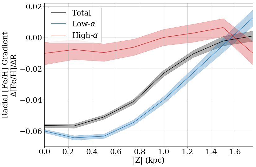
We measure the median metallicity profile for the disk by first separating stars into bins of , and then calculating a running median [Fe/H] for each bin of data points with an overlap of 50%, sorted by Galactocentric radii. We do this for the total stellar population and repeat the analysis for the high- and low- samples described in Section 2.2 separately. The resulting radial median metallicity profiles are shown in Figure 13 and quantified in Table 1.
The total sample (Fig. 13 top row, Table 1) shows a negative metallicity gradient close to the Galactic plane, which flattens out at small radii. Moving above the plane, the slope of the gradient flattens until it becomes slightly positive at kpc.
The low- disk (Fig. 13 middle row) shows a steep metallicity gradient everywhere, notably missing the flattening in the inner Galaxy seen in the total population. The low- disk’s metallicity gradient flattens with height much like the total population.
The high- disk (Fig. 13 bottom row) exhibits a much flatter or slightly positive metallicity profile whose slope does not change significantly with . The high- sequence effectively ends at kpc (shown previously in Figure 8, meaning there are not enough high- stars in the outer Galaxy to constrain the metallicity profile past kpc.
The total disk looks like the high- profile near the center of the Galaxy, and matches the low- profile in the outer Galaxy. This is due to the relative weights between these two populations at different locations: as shown in Section 3.2, the inner region of the Galaxy is dominated by the high- sequence, and the outer region is mostly low- stars.
For each median metallicity profile, we quantify the gradient by fitting a straight line to stars with Galactocentric radius kpc, where the profile reasonably approximates a single line. The best-fit slope for each profile is shown in Figure 14 against height above the plane , and tabulated in Table 1. The total population and the low- population have steep negative profiles in the outer Galaxy, which approach zero as it moves above the plane. The high- slope is close to zero everywhere. Note that if we change the definition of our measured gradient and instead fit without the radial limit of ( kpc), the high- population show a slight positive gradient, consistent with other studies (e.g., Vickers et al., 2021).
These results are generally consistent with previous results from a variety of methodologies. We measure a slope of dex kpc-1 for the total population close to the Galactic plane ( kpc). Using previous data releases of APOGEE, Feuillet et al. (2019) measured the slope of the low- metallicity gradient to be dex kpc-1. Using open clusters as tracers, Donor et al. (2020) measured a radial gradient of dex kpc-1 with APOGEE DR16 data, and Myers et al. (2022) measured dex kpc-1 with DR17. Using Gaia DR3 data, Gaia Collaboration et al. (2022) measured a slope of dex kpc-1 for their bin closest to the Galactic plane. Additional studies use Cepheid stars as tracers and find similar results, with Genovali et al. (2014) reporting dex kpc-1, and Lemasle et al. (2018) reporting dex kpc-1. The large sample size, distance range, and high precision of the APOGEE DR17 sample enable us to map the radial, vertical, and -dependence of the metallicity gradient in unprecedented detail. Differences between tracer populations used may explain the slight differences among previous results — e.g., Cepheids tend to be young stars that are more concentrated to the mid-plane, which alone results in a steeper vertical gradient.
These findings are also generally consistent with Hayden et al. (2014), who measured the metallicity gradients as a function of position ( and ) in the disk and documented a relatively flat gradient near the center of the Galaxy, a steeper gradient farther out in the disk, and generally flat gradients for the high- population (Hayden et al., 2014, Table 2). Our data set is significantly larger than that of Hayden et al. (2014), with the inclusion of Southern Hemisphere observations, which leads to better spatial coverage in both the inner and outer regions of the Galaxy and less sensitivity to potential systematics. This may be why our radial gradient dex kpc-1 is slightly shallower than the dex kpc-1 from Hayden et al. (2014) for a comparable spatial zone.
Numerical simulations from Rahimi et al. (2014) reproduce similar gradient trends where the radial metallicity gradients flatten with increasing . Notably, they attribute the slight positive gradient of the Milky Way’s thick disk to the flaring of younger populations at large radii. The vertical flaring of the mono-age, mono-abundance disk has been documented extensively in other studies as well (e.g., Minchev et al., 2015; Bovy et al., 2016; Mackereth et al., 2017; Lian et al., 2022a; Gaia Collaboration et al., 2022; Robin et al., 2022)).
| (kpc) | Total | Low- | High- |
|---|---|---|---|
| 0.0 | -0.056 0.001 | -0.06 0.001 | -0.01 0.007 |
| 0.25 | -0.057 0.001 | -0.064 0.001 | -0.008 0.006 |
| 0.5 | -0.051 0.001 | -0.063 0.001 | -0.01 0.006 |
| 0.75 | -0.041 0.002 | -0.054 0.002 | -0.006 0.005 |
| 1.0 | -0.023 0.002 | -0.04 0.002 | -0.0 0.005 |
| 1.25 | -0.01 0.002 | -0.023 0.003 | 0.003 0.006 |
| 1.5 | -0.002 0.003 | -0.005 0.005 | 0.006 0.006 |
| 1.75 | 0.001 0.003 | 0.013 0.005 | -0.01 0.007 |
The models of Johnson et al. (2021), which incorporate radial and vertical redistribution of stars based on a hydrodynamical cosmological simulation of a Milky Way-like galaxy, also show a radial metallicity gradient that flattens with increasing .
The vertical median metallicity profile of the disk is shown in Figure 15 and Table 2, calculated in the same way as the radial gradients. The best slopes for all stars kpc are shown in Figure 16 and Table 2. Consistent with Gaia Collaboration et al. (2022), we find the gradients in the disk to be vertically symmetric. The slope measured above the disk () does not differ significantly from the slope measured below the disk (). The total population has a steep negative vertical gradient close to the center of the Galaxy ( kpc), which flattens moving out in radius. This is generally true for the low- population as well, although the innermost parts of the Galaxy ( kpc), show a very flat profile, possibly due to the bulge or bar. The high- population has a shallow negative gradient everywhere, which does not significantly change with radius. Beyond kpc, the vertical gradient for the total, high- and low- populations are all close to zero.
This is also consistent with previous studies (e.g., Hayden et al., 2014, Table 1), where the vertical metallicity gradient approaches 0 as radius increases. Near the solar neighborhood, we report a vertical median metallicity gradient of dex kpc-1. Hayden et al. (2014) report a gradient of dex kpc-1 in a comparable spatial zone. For the thick disk, Carrell et al. (2012) measured a vertical metallicity gradient of , using stars close to the solar neighborhood with heights , consistent with our measurement of near the solar neighborhood for the high- population.


| (kpc) | Total | Low- | High- |
|---|---|---|---|
| 0.0 | -0.4 0.053 | -0.565 0.063 | -0.126 0.042 |
| 2.0 | -0.471 0.015 | -0.616 0.027 | -0.121 0.012 |
| 4.0 | -0.462 0.01 | -0.753 0.021 | -0.084 0.009 |
| 6.0 | -0.444 0.011 | -0.519 0.019 | -0.1 0.013 |
| 8.0 | -0.296 0.009 | -0.265 0.013 | -0.119 0.013 |
| 10.0 | -0.153 0.007 | -0.145 0.008 | -0.062 0.015 |
| 12.0 | -0.09 0.007 | -0.094 0.007 | -0.075 0.027 |
| 14.0 | -0.05 0.009 | -0.049 0.009 | -0.115 0.071 |
| 16.0 | -0.066 0.017 | -0.067 0.017 | -0.033 0.792 |
| 18.0 | -0.072 0.04 | -0.072 0.041 |
Examining the Galaxy’s metallicity profile as a function of age provides a direct link to the evolution history of the disk. Figure 17 shows the radial (top panel) and vertical (bottom panel) metallicity profile for the low- disk only, separated into bins of stellar age. In both cases, the slope of the profile flattens with increasing age. This trend is also seen in Anders et al. (2023), using a similar APOGEE sample with different age and distance estimates. The flattening of the metallicity gradients with age is the opposite of what is predicted by a pure inside-out growth of the Galaxy (e.g., Matteucci & Francois, 1989; Bird et al., 2013), where the gradient in the interstellar medium is expected to flatten out over time (e.g., Pilkington & Gibson, 2012; Gibson et al., 2013; Mollá et al., 2018). The opposite trend, seen here, is commonly attributed to be a signature of radial migration (e.g., Wang & Zhao, 2013; Magrini et al., 2016; Minchev et al., 2018; Vickers et al., 2021; Anders et al., 2023). However, an alternate explanation is also presented in Chiappini et al. (2001), where a disk formed from pre-enriched gas starts with an initially flat metallicity gradient that steepens over time.


3.5 Metallicity Distribution Function

While the radial and vertical median metallicity gradients in the disk reveal interesting general trends, more insights can be gleaned from the full metallicity distribution function (MDF) at different locations in the disk. Specifically, the spread and shape of the underlying MDF can be crucial for characterizing the complex history of the disk more accurately.
Figure 18 demonstrates how the metallicity distribution function varies with radius for samples at different vertical slices, from closest to the Galactic plane (top panel) to furthest beyond (bottom panel). Every third row is annotated with tick marks denoting the 25th, 50th (median), and 75th percentile of that row’s distribution, for the total sample (white), low- (blue), and high- (red) samples separately. The diamond point is the peak (or mode) of the distribution. At all heights, the characteristic metallicity (whether median or mode) decreases with radius for the total and low- populations, but stays roughly constant for the high- population.
At smaller radii, there is little overlap between the low- and high- MDF. In fact, the high- population alone is what creates the metal-poor tail of the total MDF. Just outside the solar neighborhood ( kpc), the MDF of the high- and low- populations overlap chemically. Moving above the plane, this overlap starts closer to the center of the Galaxy, around kpc at kpc.
The shape of the MDF changes as a function of radius; close to the center of the Galaxy, the total and low- distribution is heavily skewed towards lower metallicities (the peak trends right of the median), and in the outer Galaxy the distribution is skewed towards higher metallicities (the peak is left of the median). This is consistent with the trend seen in previous studies (e.g., Anders et al., 2014; Kordopatis et al., 2015b; Hayden et al., 2015; Loebman et al., 2016; Katz et al., 2021).
The high- MDF is consistently broader than the low-, has a shallower characteristic gradient, and shows less of a skewness trend with radius; the peaks (diamond points) are closer to the median (center tick mark) in general. Stars in the low- sample transition from being negatively skewed in the inner Galaxy to positively skewed in the outer Galaxy (as shown in Figure 19). However, this trend is not seen as strongly in the high- disk, even at similar Galactic heights as the thin disk. Because the high- population is generally older, this could imply that the high- sample is more “mixed” vertically, meaning the birth location of stars tend to be farther away from their present-day location, largely because they have had more time to migrate radially.
Kordopatis et al. (2015b) also observed an overabundance of metal-rich stars in the solar neighborhood using data from the RAVE survey, and link it to radial migration. Hayden et al. (2015) observed this same trend in APOGEE and present a simple model to show that radial migration could explain the change of the MDF shape with radius, because more stars migrate outward from the inner disk than vice versa. Loebman et al. (2016) and Johnson et al. (2021) show that this explanation succeeds quantitatively in models with realistic radial migration from cosmological simulations. These studies also show that the excess metal-rich tail in the MDF disappears at high , in agreement with the results of Figure 18 and Hayden et al. (2015).
Some simple statistics can be measured to more fully characterize the MDF as a function of radius, as shown in Figure 19 for the case of the low- disk close to the Galactic plane (equivalent to the top panel of Figure 18). The top right plot shows three definitions for a characteristic value for [Fe/H]; the mean, median, and peak of each distribution as a function of radius. While these values are similar, they are not identical, meaning the measured metallicity gradient of the disk will depend on the parameterization of [Fe/H] chosen. In the inner disk, the peak [Fe/H] is up to 0.1 dex higher in metallicity than the mean and median, due to the distributions being skewed metal-rich. In the outer disk, the peak is preferentially more metal-poor. Therefore, a metallicity gradient measured using the peak metallicity as a tracer will have a steeper slope than a gradient measured with the mean metallicity for the same group of stars.
The middle right panel in Figure 19 quantifies the spread of each distribution with radius, as total standard deviation . The outer regions of the disk ( kpc) are characterized by narrower distributions with less overall spread, whereas the inner disk MDFs span a larger range of metallicities.
The bottom right panel quantifies the skewness of each distribution with radius. The MDF in the inner regions of the disk it is negatively skewed, and in the outer regions it is positively skewed, quantifying the trend seen earlier Figure 18.
3.6 Age Gradients
The present-day distribution of stellar ages can act as an interesting snapshot as to what the Milky Way might have looked like at different points in time, while also documenting how stars might move and migrate away from their radius of birth.
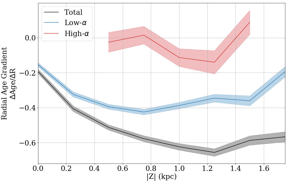
The radial median age profile of the Milky Way is presented in Figure 20, identical to the way the metallicity gradients in Section 3.4 were calculated. The best-fit slope for each profile is shown in Figure 21, once again calculated only using stars with kpc where the profile reasonably approximates a straight line.
The median age of the high- population is generally the same everywhere, with a slope close to 0 at any height above the plane. We note that the median age observed here, Gyr, is likely too young due to selection effects and the limitations of our age sample, including the metallicity cut of [Fe/H] dex discussed in Section 2.4.
The total and low- stellar populations have a negative radial median age gradient in the outer Galaxy, while in the inner Galaxy the profile flattens out. The measured slope is flattest close to the disk (), and becomes negative moving above the plane. The total and low- stellar populations have a vertical gradient that varies with radius as well. The vertical gradient is steeper closer to the center of the Galaxy, and flatter at large radii, similar to the vertical metallicity gradient. Unlike the high- sample, the majority of stars in the low- disk have metallicity [Fe/H] and are therefore more robust against potential biases caused by the sample selection (see Figure A.1).

3.7 Age Distribution Function

As before with metallicities, more information lies in the shape of the age distribution function at different locations in the Galaxy rather than the gradient alone. Figure 22 depicts the age distribution function (ADF) as a function of Galactocentric radius for different heights in the disk. Close to the Galactic plane (left panel), the peak age of the total population gradually declines, peaking around 7.5 Gyr near the Galactic center and 3 Gyr near the solar radius and outward. The spread of the ADF is fairly broad, spanning up to 5 Gyr at all radii. In the outer Galaxy, the ADF is preferentially skewed toward older ages. Katz et al. (2021) found the ADF skewed towards younger ages in the inner Galaxy, and skewed towards older ages in the outer Galaxy, but they limited their investigation to just the low-, thin disk sample.
Farther above the Galactic plane (middle and bottom panels of Fig. 22), the profile does not show a single gradient, but rather has a slight positive age gradient until kpc which transitions into a negative gradient at larger . After kpc, the gradient flattens out. We caution that this flattening of the gradient at large may be artificially induced by the lack of [Fe/H] stars in our sample when dealing with ages imposed by the sample cuts described in Section 2.4.
Separating further into the low- and high- samples reveals slightly different trends. Close to the Galactic plane (top panel), and in the inner Galaxy, there is some minimal overlap between the low- and high- samples, but near the solar neighborhood and outward, the ADF is more bimodal and there is more separation between the high- and low- ADF. At all radii, the low- sample has a narrower distribution, and transitions from being skewed toward younger ages in the inner Galaxy to being skewed toward older ages in the outer Galaxy. This is similar behavior to the MDF in Figure 18, and also seen by Katz et al. (2021). Farther above the plane, there is more overlap between the low- and high- samples in the inner Galaxy, but there is still little overlap at larger radii.
Despite the similarities in these representations of the ADF to the corresponding ones for MDFs, we caution that the age uncertainties (typically dex) are significant relative to the total spread, which is not the case for the [Fe/H] measurements.
3.8 Age-Metallicity Relation

The relation between stellar age and metallicity has long been sought after to help constrain chemical evolution models (e.g., Twarog, 1980; Edvardsson et al., 1993). In a simple “closed box” system, the metallicity of stars should increase over time, as each generation of stars enriches the interstellar gas from which subsequent generations are born. The actual scenario is much more complex, depending on gas inflow and outflow rates, supernovae yields, stellar migration, and the positionally variable star formation history of the Galaxy. Observations of the age-metallicity relation in the Milky Way include the effects of all of these processes, and they therefore provide a powerful constraint for chemical evolution models to reproduce across different locations in the Galaxy.
Previous studies have found significant scatter in the age-metallicity relation (AMR) near the solar neighborhood, where stars with a single age span a wide range of metallicities, which cannot be attributed to observational errors alone (e.g., Casagrande et al., 2011; Bergemann et al., 2014; Aguirre et al., 2018; Lin et al., 2018; Grieves et al., 2018; Sahlholdt et al., 2022; Xiang & Rix, 2022; Anders et al., 2023). The AMR also varies with Galactic location, making it difficult to constrain a single relation that fits the whole disk (e.g., Hasselquist et al., 2019; Feuillet et al., 2019; Casamiquela et al., 2021; Lian et al., 2022b; Anders et al., 2023).
The AMR for our sample of stars in the Milky Way disk is shown in Figure 23. The data are split into bins of radius (columns), and height (rows), to demonstrate how the age-metallicity relation varies across Galactic location. Points are colored by -element abundances, which are known to be correlated with age, although the exact trend depends on Galactic position (e.g., Haywood et al., 2013; Nissen, 2015; Bedell et al., 2018; Feuillet et al., 2018; Hasselquist et al., 2019; Lian et al., 2022b, see also Section 3.9). The median trend across different bins in age is tracked as black square points to help guide the eye. Note that the x-axis (stellar age) has been reversed so that older stars are on the left, better expressing the forward flow of time. The x-axis is also presented in log space, which is more representative of the uncertainties in our age estimates (Section 2.4). One can also read each panel rotated 90∘ to see the distribution of log(age) at fixed [Fe/H].
Consistent with previous studies, there is significant scatter around the age-metallicity relation near the solar neighborhood. There is a slight gradient in -element abundances within that spread; nearly everywhere in the Galaxy, higher-metallicity stars are relatively more -poor.
The age-metallicity relation has less scatter moving towards the inner Galaxy (left column), and above the plane (top row). If the spread in this relation is due to the radial migration of stars, this implies that the in-situ age-metallicity relation of the inner galaxy has been more preserved, and less contaminated by migrated stars; or in other words, more stars migrate outwards than inwards in the Galaxy. This is perhaps not surprising; dynamically, stars in the inner Galaxy migrate outwards, and stars in the outer Galaxy migrate inwards (e.g., Sellwood & Binney, 2002). The inner Galaxy is denser than the outer disk, so if one assumes the same rate of migration across all radii, more stars would migrate outwards simply because more stars start in the inner Galaxy. The age-metallicity relation shown in Sahlholdt et al. (2022) also shows a lower dispersion for the inner regions of the disk (their “Pop C” sample) using GALAH data.
The AMR is steepest in the inner Galaxy, and flattens moving out in radius. In all panels, the age-metallicity relation flattens out at young stellar ages, perhaps indicating that chemical equilibrium has been reached, where the inflowing gas dilutes the ISM at the same rate as it is being enriched (e.g., Dalcanton, 2007; Finlator & Davé, 2008; Weinberg et al., 2017). In the inner disk, the equilibrium metallicity is higher than the equilibrium metallicity reached in the outer disk and moving away from the midplane. Equilibrium seems to have been reached sooner (at older stellar age) in the outer disk than the inner disk.

There is a notable inversion of the AMR at large radii in the Galaxy, where older stars trend more metal-rich than the younger stars in the sample. This has been reported before in previous studies (e.g., Anders et al., 2014; Feuillet et al., 2018; Hasselquist et al., 2019; Lian et al., 2022b). The cosmological simulations of Lu et al. (2022) explore the possible origins of such an inversion, suggesting that it could be the signature of interactions with a satellite galaxy like the Sagittarius dwarf, and radial migration notably widens the apex.
A recent study from Xiang & Rix (2022) documented a disjointed age-metallicity relation for the sum of the total disk, and suggested that the two-infall scenario or a major merger is responsible. In our results, we see some evidence of bimodality in Figure 24, which is a contour map of the point density distribution in Figure 23. In the inner Galaxy ( kpc), the age-metallicity relation has two separate peaks.
3.9 Age-Alpha Relation and Chemical Clocks
While no clear correlation between age and metallicity relation exists near the solar neighborhood, better correlation has historically been found between age and -element abundances (e.g., da Silva et al., 2012; Haywood et al., 2013; Bensby et al., 2014), leading some to use -elements as a chemical clock, substituting their abundances when stellar ages are not readily available. Even so, the [Mg/Fe]-age correlation has been found to vary across the Milky Way’s disk (e.g., Aguirre et al., 2018; Feuillet et al., 2018; Katz et al., 2021; Vázquez et al., 2022), extending the metaphor to imply that chemical clocks run in chemical “time zones” throughout the Galaxy. Reproducing this variation has been considered a strong constraint on chemical evolution models (e.g., Haywood et al., 2013; Spitoni et al., 2019a; Johnson et al., 2021).
Figure 25 shows the relation between age and [Mg/Fe] as a contour plot at various locations throughout the disk. The distribution is double-peaked in nearly all panels, with the older, low- population most prevalent above the disk and in the inner Galaxy. Near the solar neighborhood and outward, the relation of the low- sequence is relatively flat, with a large spread in ages corresponding to a small range of [Mg/Fe] abundances. This is consistent with the findings of Haywood et al. (2013) and Feuillet et al. (2018). In the inner Galaxy, a small range in [Mg/Fe] abundances corresponds more tightly with a smaller range in age, a phenomenon that applies, though differently, to each the high- and low- groups. As in Haywood et al. (2013), we observe some age overlap between the two sequences, implying that the low- sequence in the outer disk began forming stars while the high- disk was concurrently still forming stars in the center of the Galaxy.
For the low- sequence, there is some evolution with Galactic position. The low- stars are older and more -poor near the center of the Galaxy. In the outer Galaxy, the sequence is more -enhanced and generally younger, although covering a larger spread in ages. Above the plane ( kpc), the low- sequence is more -enhanced.
The high- sequence stays generally in the same location on this diagram regardless of position in the Galaxy. This is similar to the trend seen in Figure 8 and 10, where the locus of the low- sequence changes significantly with Galactic position while the high- sequence stays largely in the same location.
In the kpc and low- zones, the log(age) distribution is bimodal even within the low- sequence. This could be evidence for a three-phase star formation history. Sahlholdt et al. (2022) report a similar distribution in the age-metallicity relation of their “Pop A” sample, which probes a similar location in the disk. The younger peak in log(age) appears similar to the recent starburst 2-3 Gyr ago detected independently in Isern (2019) and Mor et al. (2019), although we note that this is the first time to our knowledge that it has been detected in APOGEE data. This recent starburst is thought to be linked with the Sagittarius dwarf spheroidal galaxy’s most recent perigalactic passage through the Milky Way’s disk (Ruiz-Lara et al., 2020; Laporte et al., 2019; Antoja et al., 2020). The uncertainties in our age estimates are not negligible, but are likely not responsible for this bimodality. Larger uncertainties would blur out the distribution and decrease the observed bimodality.
We remind the reader that using different estimates for stellar ages can change our results. Alternate versions of this figure using different age catalogs are shown in Appendix A to emphasize this point.

3.10 Chemical Evolution via Chemical Tagging

If a group of stars was born together in the same location and at the same time, they should have identical chemical abundances ([Fe/H] and [Mg/Fe] in our case). This is the basic assumption behind “chemical tagging”, used to identify stellar siblings that have been redistributed throughout the Galaxy despite being born together (e.g., Freeman & Bland-Hawthorn, 2002; Hawkins et al., 2015; Ting et al., 2015; Price-Jones et al., 2020; Buder et al., 2021). Under this assumption, we can potentially track radial migration and the spatial redistribution of a stellar population over time, as well as look at the enrichment history of an area of the Galaxy for fixed metallicity.
Figure 26 shows this evolution for stars close to solar metallicity ( [Fe/H] dex). The present-day radial distribution (x-axis) and [Mg/Fe] abundance (y-axis) is shown for different bins in stellar age (line color) for both the low- (solid lines) and high- populations as the contour containing 75% of all points in that bin. Stars at the same age and metallicity should all have same [Mg/Fe] abundance. If stars did not move from where they were born, we would expect to see a tight clump in this space. If stars migrate significantly over time, the shape of the clump should spread out to a broader range of radii, but keep the same [Mg/Fe] abundances (or a “flat slope” in [Mg/Fe]). If the slopes were not flat, it may be indicative of different enrichment histories for different parts of the Galaxy; suggesting a violation of the assumption that stars with the same metallicity and age were born roughly in the same place.
The young, -poor stars in Figure 26 currently reside in a relatively confined clump in radius and [Mg/Fe] as expected ( kpc). As stellar age increases, the shape of the clump widens to cover a broader range in radius ( kpc) while the [Mg/Fe] abundance remains confined. The high- sequence does not show this evolution in radial width with time, but notably does not include enough young stars to properly trace this. As shown in Figure 9, high- stars tend to be old.
As stellar age decreases, the median [Mg/Fe] value of each subpopulation decreases for both the low- (solid lines) and high- (dashed lines) populations. In the low- population, the median value of [Mg/Fe] decreases from [Mg/Fe] = 0.05 in the oldest age bin () to [Mg/Fe] in the youngest age bin (). This tracks the chemical evolution of a location in the Galaxy, as Type Ia supernovae begin “diluting” the interstellar medium with iron, thereby decreasing the overall [Mg/Fe] ratio over time.
4 Discussion
Using large samples of stars to map the Milky Way in different parameter spaces using metallicity, -element abundances, and age, as demonstrated here, has the potential to place strong constraints on chemical evolution models and reveal the major processes which shaped our Galaxy. Directly comparing our results with specific chemical evolution models is beyond the scope of this paper, but in this discussion section we qualitatively compare our results with predictions from the leading classes of chemical evolution models discussed in the Introduction; the “two-infall”, “superposition”, and “clumpy formation” scenarios.
The underlying assumption necessary to interpret these results is that in a well-mixed interstellar medium, stars formed at the same time and the same place in the Galaxy will have the same chemical abundances (both metallicity and -elements). Under this assumption, a spread in abundance at present day for stars at a given age at the same location, whether bimodal or not, can only be produced if stars have moved away from their birth location.
4.1 Superposition and Radial Migration
The “superposition” class of evolution models (e.g., Schönrich & Binney, 2009a, b; Minchev et al., 2013, 2014, 2017; Johnson et al., 2021) explain the observed chemical bimodality in the solar vicinity as the superposition of evolutionary tracks for stars born at different Galactocentric radii, with the stars having reached their present-day location in the solar neighborhood through radial migration. Several predictions made by these superposition chemical evolution models are seen in our results.
The metallicity gradient flattening with age (Figure 17) is predicted by radial migration (e.g., Sellwood & Binney, 2002; Roškar et al., 2008; Wang & Zhao, 2013; Hayden et al., 2015; Mackereth et al., 2017; Frankel et al., 2018, 2020; Vickers et al., 2021; Lian et al., 2022b). If stars are formed in-situ with a steep metallicity gradient, that gradient will flatten over time as metal-rich inner Galaxy stars migrate outwards and metal-poor outer Galaxy stars migrate inwards, skewing the metallicity distribution at either end of the Galaxy. The older stars in our sample show a flatter gradient than the younger stars; in agreement with this scenario.
The shape of the metallicity distribution function at different locations in the Galaxy (Figures 18 and 19), specifically the skewness or asymmetry of the MDF, can be a sign of radial migration if a population of stars has a metal-rich tail (e.g., Hayden et al., 2015; Kordopatis et al., 2015b; Loebman et al., 2016)). Our data show a skewed MDF in Figure 19, where the inner region of the disk is negatively skewed, and the outer region of the disk is positively skewed. This trend is commonly attributed to radial migration, whereby migrating stars become the metal-rich tails in the MDF at different locations (e.g., Schönrich & Binney, 2009a, b; Roškar et al., 2008; Kordopatis et al., 2015b; Loebman et al., 2016; Johnson et al., 2021). The metal-poor tail in the inner Galaxy’s MDF is likely attributed to a spread in ages between the stars, as is predicted by even closed-box chemical evolution tracks when any given location in the Galaxy becomes enriched over time (e.g., Romano & Starkenburg, 2013; Vincenzo et al., 2014; Weinberg et al., 2017; Toyouchi & Chiba, 2018). The metal-rich tail of the outer Galaxy’s MDF is more difficult to explain with a traditional chemical enrichment track, which leaves radial migration as the most likely culprit.
The inversion in skewness in the MDF occurs around kpc in our data. This could be linked to the Outer Lindblad Resonance (OLR) of the Milky Way disk; a resonance with the Galactic bar driving different dynamical effects throughout the disk, one of which is radial migration (Halle et al., 2015; Michtchenko et al., 2016; Dias et al., 2019; Khoperskov et al., 2020b). Using Gaia data, Khoperskov et al. (2020a) estimates the OLR to be located at a Galactocentric radius of around 9 kpc. Khoperskov et al. (2020b) uses a high-resolution N-body simulation to investigate the relationship between the OLR and radial migration, and find that stars from the inner Galaxy migrating outwards become “trapped” in the OLR. When the rotation period of the bar slows down, those stars can escape and migrate farther out. The trapping effect of the OLR could also explain the build-up of metal rich stars at kpc in Figures 5 and 6.
We also see signs of radial migration in the age-metallicity relation shown in Figure 23. Around the solar neighborhood, there is significant scatter about the age-metallicity trend. If the interstellar medium is always well-mixed, the large spread in metallicity for stars of a given age must mean that some of these stars were not born at their present-day location. This is another consequence of radial migration predicted by the superposition class of models, which explain the spread by emphasizing the difference between the present-day locations of stars and their birth radii (e.g., Schönrich & Binney, 2009a; Wang & Zhao, 2013; Minchev et al., 2013; Lian et al., 2022b). While any location in the Galaxy should start with a tight age-metallicity relation, migration will blur the present-day relation as metal-rich stars from the inner disk move outward and contaminate the more metal-poor outer disk. Radial migration is most efficient in the plane of the disk, therefore these models predict less spread in the age-metallicity relation at larger vertical heights, an effect also seen in our data.
The turnover in the age-metallicity relation, seen in Figure 23 and in Hasselquist et al. (2019), can also be explained through radial migration. The older, metal-rich stars were likely formed in the inner Galaxy, and migrated outwards to where they are found today, contaminating the age-metallicity relation. An alternate explanation could be the dilution of the ISM from pristine gas infall, lowering the metallicity of a previously-enriched area of the Galaxy (e.g., Spitoni et al., 2019a; Lu et al., 2022). However, in this scenario, it is predicted that both the high- and low- tracks in metallicity would still decrease with stellar age, with the post-dilution low- track beginning at a lower metallicity than the high- track at the same time (e.g., Spitoni et al., 2019a). That predicted trend is not obvious in our data, and the large spread in metallicity at a given age favors a radial migration explanation. Lu et al. (2022) further explore the origin of such a turnover using cosmological simulations, and find that even when the turnover in the age-metallicity relation can be directly linked to the infall of a satellite galaxy, radial migration can widen the shape of the peak.
Vertical motions should also be considered. In the age- relation of Figure 25, a population of stars with the same age and in the same present-day location can have a large spread in [Mg/Fe], most dramatically seen in the inner Galaxy ( kpc). This violates the underlying assumption mentioned earlier, meaning stars must have moved around to create that spread. However, in this case, radial migration is an unsatisfactory explanation, as stars from the outer Galaxy migrating inward is expected to be a less frequent occurrence than the other way around, simply a consequence from the density profile of the Galaxy (e.g., Sellwood & Binney, 2002). Instead, the vertical motion of stars could result in the observed spread if stars born above the mid plane are currently found near . Even stars formed above the plane will inevitably have vertical motions that cause their orbits to cross the plane, meaning this could be a natural consequence of a star’s vertical orbit. Related vertical motions could be linked with dynamical heating (e.g., Spitzer & Schwarzschild, 1951; Barbanis & Woltjer, 1967; Lacey, 1984; Mackereth et al., 2019) or the “upside-down” formation of the disk (e.g., Toth & Ostriker, 1992; Quinn et al., 1993; Hänninen & Flynn, 2002; Brook et al., 2004; Freudenburg et al., 2017; Bird et al., 2013, 2021). Using a quantity like guiding radius () and maximum height calculated from parameterized stellar orbits, instead of the present-day and we use here, may remove contamination by thick disk stars currently “passing through” the thin disk from these figures. Some studies, including Boeche et al. (2013), Katz et al. (2021), and Spitoni et al. (2022a), have looked at these quantities, and found similar overall trends.
The evolution of radial distribution with stellar age seen in Figure 26 is yet more evidence for radial migration. The youngest, low- stars indicate that for a population of fixed age, [Fe/H], and [Mg/Fe], they are expected to be born at a similar radius in the Galaxy. As stellar age increases, the population redistributes into a larger range of , showing that stars migrate radially over time. The high- stars, which cover a similar range in Galactic radius despite a wide window in age ( age Gyr), may suggest an “upper limit” on the efficiency of radial migration and the timescales over which stars can migrate on average; see e.g., Frankel et al. (2020) and Lian et al. (2022b) for such an analysis. Similarly, the relative distribution of stars within the low- contours may hint at the importance of direction in radial migration (i.e., what fraction of stars migrate outwards instead of inwards), although such a discussion is beyond the scope of this work.
This wide variety of results suggests that significant stellar migration occurs in the Milky Way disk, most influencing the trends seen close to the Galactic plane and at larger radii. However, there are open questions remaining about the nature of the inner disk, where an apparent bimodality exists that is not easily explained by migration models.
4.2 Two-Infall or Major Merger
The “two-infall” class of evolution models (e.g., Chiappini et al., 1997, 2001; Lian et al., 2020a, b, c; Spitoni et al., 2019a, 2020, 2021, 2022a) suggest that the two sequences in [Mg/Fe]-[Fe/H] space formed sequentially in time. Under this scenario, the thick disk was formed first during the initial collapse of the Galaxy, and after some time delay a second infall of gas fed the creation of the thin disk. These models predict several of the observed trends in our results, most notably in areas where radial migration is not as efficient, including the inner Galaxy and at greater heights above the Galactic plane.
Figure 8 shows that the -bimodality persists throughout the majority of the disk. This is significant because while the “superposition” class of chemical evolution models can produce the low- “sequence” and broad distribution of [Mg/Fe] in the solar neighborhood using only radial migration (e.g., Schönrich & Binney, 2009a, b; Minchev et al., 2013, 2014; Nidever et al., 2014; Sharma et al., 2021a; Johnson et al., 2021), radial migration is known to be most efficient close to the Galactic plane and in the outer disk. Therefore, the bimodality in other parts of the Galaxy is more difficult to explain with radial migration alone. Previous studies by Freudenburg et al. (2017) and Zasowski et al. (2019) report that the shape of the MDF and the [Mg/Fe]-[Fe/H] trends seen in the inner disk ( kpc) could be modeled well using a single evolutionary track in an “upside-down” disk formation model.
Our results are consistent with this in the [Mg/Fe]-[Fe/H] realm, but when expanded to ages, we show that two distinct tracks of [Mg/Fe] are observed even in the inner Galaxy. This is also reported in Queiroz et al. (2021).
Near the solar neighborhood, radial migration models predict bimodality by explaining the high- sequence as contaminants from the inner Galaxy; due to the intrinsic density profile of the Galaxy, more stars are expected to migrate outwards than inwards, so the inner Galaxy should display less contamination from the low- sequence. This is in contradiction with our findings, where the -bimodality persists throughout the majority of the disk. Johnson et al. (2021) also report that the bimodality reproduced by their superposition model is weaker than the observed bimodality in the Milky Way; in particular, the model overproduces intermediate- stars compared to observations. Chen et al. (2022) find greater success in producing bimodality with radial migration. However, a two-infall (or multi-infall) model may be needed to explain the bimodality in the inner Galaxy.
The age-metallicity relation in Figure 23 produces some trends that are better explained by the two-infall model than by radial migration. Minchev et al. (2013, 2014) report that while the scatter around the age-metallicity relation can be attributed to radial migration, the overall slope is only weakly affected. In our data, consistent with other recent studies (Feuillet et al., 2019; Hasselquist et al., 2019), the slope of the age-metallicity relation varies significantly with Galactic radius. This is reproduced with a two-infall model, where the low-, post-infall disk has a shallower slope in the age-metallicity relation compared to the high- population, due to the continuous inflow of gas diluting the disk that was not present during the formation of the original high- disk (Spitoni et al., 2019a, 2020, 2021).
The apparent disk bimodality is not only observed in [Mg/Fe]-[Fe/H] chemistry, but also in the age-metallicity relation. Recent work by Xiang & Rix (2022) show a disjointed age-metallicity relation for the sum of the total disk, which is only possible to reproduce in a two-infall scenario or with a major merger event. In our study, the age-metallicity relation as a function of Galactic position (Fig. 23) also shows a possible bimodality, most apparent in the kpc range of the inner disk.
The age-[Mg/Fe] relation in Figure 25 is perhaps more convincing evidence for the two-infall model, with clear bimodality in the relation persisting across nearly the entire disk. In the outer disk (), there appears to be an additional bimodality within the low- sequence, suggesting a three-phase star history similar to that detected in Sahlholdt et al. (2022) using a sample of stars from the GALAH survey. The uncertainties in our age estimates are not negligible, but are likely not responsible for this bimodality. Larger data uncertainties would blur out the distribution and decrease the observed bimodality. Due to the age uncertainties, the “true” age bimodality in the Milky Way may be stronger than what is shown in our analysis. The peak of our “third” starburst is around 2-3 Gyr, consistent with the recent burst Isern (2019) and Mor et al. (2019) report, possibly linked to the most recent interaction with the Sagittarius dwarf spheroidal galaxy as it passed through the disk (e.g., Ruiz-Lara et al., 2020; Laporte et al., 2019; Antoja et al., 2020)
In the age-[Mg/Fe] relation, the age overlap between the high- and low- sequences are impossible to explain with a single evolutionary track. In this interpretation, we do caution that if the transition from high- to low- is fast, uncertainties in age determination could produce an artificial impression of age overlap. Haywood et al. (2013) also detects an overlap in age, and claim that the dichotomy in the solar neighborhood can be reproduced by the two-infall scenario, and that little to no radial migration is needed.
For the inner disk, the spread in [Mg/Fe] for a given age is likely due to the vertical motions of stars as discussed previously in Section 4.1. However, if the spread was purely from vertical blurring, a continuous spread would be expected, and not the bimodal distribution seen here.
As discussed in Appendix A, the choice of stellar age catalog does significantly change the appearance of the age-[Mg/Fe] relation across the disk, suggesting that stellar age estimates are not yet robust enough to draw strong conclusions from this relation. Nevertheless, several of the key features observed here (the age overlap and the bimodality within the low- sequence) do persist across different age catalogs.
In summary, the bimodality in [Mg/Fe] and stellar ages persisting across the inner disk is not easily explained through radial migration, which is most efficient at larger radii. A multi-phase star formation history, such as those presented in the two-infall model, better predicts the trends observed in the inner Galaxy.
4.3 Clumpy Star Formation Models
The “clumpy star formation” models (e.g., Clarke et al., 2019; Beraldo e Silva et al., 2020; Amarante et al., 2020) predict that the two sequences in -element abundances formed simultaneously but in different modes: the high- sequence formed in rapidly-enriched gaseous clumps and the low- formed in a less efficient smooth disk. This clumpy phase of early disk formation is predicted by numerical simulations (e.g., Bournaud et al., 2007) and often seen in observations of high redshift galaxies (e.g., Elmegreen et al., 2005).
One major result that the clump star formation models predict is the temporal overlap between the two sequences: The low- disk starts forming at the same time as the high- sequence, meaning there should be some overlap in stellar ages between the two sequences. We see this overlap in Figure 23 and 25, where stars at around (age) Gyr span a significant range in both metallicity and -element abundances. This age overlap has also been observed in previous studies (e.g., Haywood et al., 2013; Hayden et al., 2017; Aguirre et al., 2018; Gent et al., 2022). Unfortunately, high uncertainties in age estimates could artificially produce this overlap.
The age distribution in the [Mg/Fe]-[Fe/H] plane shown in Figure 9 also possibly points to this formation scenario. As discussed in Section 3.2, the distribution of stellar ages within the low- sequence suggests that it is not a single evolutionary sequence. Stellar age is more closely correlated with [Mg/Fe] instead of [Fe/H]. A strikingly similar trend is notably predicted under the clumpy formation scenario (Clarke et al., 2019, Fig. 9).
One potential avenue for further investigating the difference between the two-infall class of models and the clumpy star formation models lies not within the Milky Way but in other galaxies. If the two-infall model is true, a chemical bimodality would only be present in galaxies that experienced significant gas infall both at early and late times, meaning it would be a rare phenomenon only affecting approximately 5% of galaxies with comparable mass to the Milky Way (e.g., Mackereth et al., 2018; Gebek & Matthee, 2022). In contrast, the clumpy star formation models predict that chemical bimodality would be more common in galaxies with comparable mass to the Milky Way, because star formation clumps are observed in more than 60% of high-redshift galaxies (e.g., Guo et al., 2015). Such an analysis could be done using spatially-resolved stellar population deconstruction of an edge-on disk, the likes of which are only recently becoming achievable observationally (e.g., Martig et al., 2021).
5 Conclusions
The large sample size, extensive spatial coverage, more complete sampling of the inner Galaxy and mid plane inaccessible to optical spectroscopic surveys, and precise abundance measurements for stars in the final data release of APOGEE can help provide strong constraints on Galactic formation and evolution models, in particular for its disk populations. We present results from the final data release of the combined SDSS APOGEE and APOGEE-2 surveys that explore the chemical and age structure of the Milky Way’s disk, measure gradients and distribution functions, and link these new observational constraints to predictions from different chemical evolution models.
Our main conclusions are as follows:
-
•
Cartography: Overall maps of the Milky Way disk exhibit negative radial age and metallicity gradients. The bar/bulge stands out as more metal-rich and -poor in the inner Galaxy compared to stars at similar radii but different azimuthal angles (e.g., Wegg et al., 2019; Zasowski et al., 2019; Hasselquist et al., 2020; Eilers et al., 2021).
-
•
[Mg/Fe] Distribution: The distribution of -element abundances reveals the chemically bimodal disk structure in the Milky Way (e.g., Fuhrmann, 1998; Bensby et al., 2005; Reddy et al., 2006; Lee et al., 2011; Hayden et al., 2015; Kordopatis et al., 2015a). The low- disk is thinner (in ) and more radially extended than the high- disk (e.g., Yoshii, 1982; Gilmore & Reid, 1983; Bensby et al., 2011; Bovy et al., 2016). The locus of the low- sequence varies with radius. Stellar ages within the low- sequence do not seem to track a true single sequence, implying a superposition of evolutionary tracks.
-
•
Azimuthal Variance of Metallicity: We find no significant evidence of large-scale azimuthal asymmetry in most of the disk, although the Galactic bar stands out as metal-rich in the mid-height plane. In the solar neighborhood, we see some coherent, non-axisymmetric structure in metallicity, although it does not obviously correlate with the spiral arms as it does in some studies (e.g., Inno et al., 2019; Poggio et al., 2022; Hawkins, 2022) .
-
•
Metallicity Gradients: The Milky Way’s full radial metallicity gradient is flat near the center of the Galaxy, and steepens farther out in radius. The high- disk displays a nearly flat metallicity profile everywhere in the Galaxy, and the low- disk has a negative gradient that is shallower at high than it is close to the plane. We measure the overall radial metallicity gradient of the disk kpc to be dex kpc-1. The overall vertical metallicity gradient of the disk at the solar neighborhood is dex kpc-1. Both the radial and vertical metallicity gradients flatten with increasing stellar age. These values are consistent with previous studies (e.g., Hartkopf & Yoss, 1982; Anders et al., 2014; Hayden et al., 2014; Frankel et al., 2019; Katz et al., 2021; Vickers et al., 2021; Gaia Collaboration et al., 2022).
-
•
Metallicity Distribution Function: The MDF of the inner Galaxy has the widest spread, but this narrows with radius. The shape of the MDF skews strongly for the low- disk, transitioning around kpc from having a metal-poor tail in the inner Galaxy to having a metal-rich tail in the outer Galaxy (e.g., Anders et al., 2014; Kordopatis et al., 2015b; Hayden et al., 2015; Loebman et al., 2016; Katz et al., 2021).
-
•
Age Gradients: Like the metallicity gradient, the age profile of the disk is flat in the inner Galaxy but transitions to a negative gradient in the outer Galaxy. The outer Galaxy’s gradient is steeper at higher for the low- population, and flat everywhere for the high- stars (e.g., Bergemann et al., 2014; Martig et al., 2016; Katz et al., 2021; Anders et al., 2023).
-
•
Age Distribution Function: The ADF for the low- disk changes in skewness similar to the MDF (e.g., Katz et al., 2021), with the inner Galaxy skewed towards younger ages, and the outer Galaxy skewed towards older ages. Above the plane kpc), there is significant overlap between the ADF of the low- and high- populations (e.g., Haywood et al., 2013; Hayden et al., 2017; Aguirre et al., 2018; Gent et al., 2022), which does not hold closer to the plane.
-
•
Age-Metallicity Relation: The AMR exhibits significant spread near the solar neighborhood, but is more tightly constrained in the inner Galaxy and at larger vertical heights (e.g., Casagrande et al., 2011; Bergemann et al., 2014; Feuillet et al., 2018). The slope of the age-metallicity relation varies with radius, and there exists a population of older, metal-rich stars around the solar neighborhood that are likely present due to radial migration (e.g., Hasselquist et al., 2019; Sahlholdt et al., 2022; Lian et al., 2022b). The age-metallicity relation suggests that the outer disk began forming low- stars while the high- sequence was still forming in the inner disk (e.g., Haywood et al., 2013; Aguirre et al., 2018; Gent et al., 2022).
-
•
Age-Alpha Relation and Chemical Clocks: The age-alpha relation appears bimodal nearly everywhere in the Galaxy. The low- sequence evolves significantly with Galactic position, while the high- sequence displays a constant trend independent of Galactic position (e.g., Haywood et al., 2013; Feuillet et al., 2018; Katz et al., 2021). There may be evidence of a three-phase star formation history (e.g., Sahlholdt et al., 2022) just outside the solar neighborhood ( kpc).
Our results suggest that radial migration is an important process in shaping the present-day appearance of the disk, especially at large radii and close to the Galactic plane. However, stellar migration alone cannot explain the bimodal nature of the -element abundances or the distribution of stellar ages in the disk. A non-continuous evolution model, such as the two-infall scenario or clumpy star formation, appears necessary to explain the trends seen in the inner Galaxy.
Acknowledgements
We would like to thank the anonymous reviewer for their useful feedback towards improving this manuscript.
J.I., C.P, J.A.H. and A.S.M gratefully acknowledge support from NSF grant AST-1909897. D.H.W. and J.A.J. gratefully acknowledge support from NSF grant AST-1909841.
T.C.B. acknowledges partial support for this work from grant PHY 14-30152; Physics Frontier Center/JINA Center for the Evolution of the Elements (JINA-CEE), awarded by the US National Science Foundation, and OISE-1927130: The International Research Network for Nuclear Astrophysics (IReNA), awarded by the US National Science Foundation.
J.G.F-T gratefully acknowledges the grant support provided by Proyecto Fondecyt Iniciación No. 11220340, and also from ANID Concurso de Fomento a la Vinculación Internacional para Instituciones de Investigación Regionales (Modalidad corta duración) Proyecto No. FOVI210020, and from the Joint Committee ESO-Government of Chile 2021 (ORP 023/2021), and from Becas Santander Movilidad Internacional Profesores 2022, Banco Santander Chile.
C.A.P is thankful for funding from the Spanish government through grants AYA2014-56359-P, AYA2017-86389-P and PID2020-117493GB-100.
Funding for the Sloan Digital Sky Survey IV has been provided by the Alfred P. Sloan Foundation, the U.S. Department of Energy Office of Science, and the Participating Institutions. SDSS acknowledges support and resources from the Center for High-Performance Computing at the University of Utah. The SDSS web site is www.sdss.org.
SDSS is managed by the Astrophysical Research Consortium for the Participating Institutions of the SDSS Collaboration including the Brazilian Participation Group, the Carnegie Institution for Science, Carnegie Mellon University, Center for Astrophysics — Harvard & Smithsonian (CfA), the Chilean Participation Group, the French Participation Group, Instituto de Astrofísica de Canarias, The Johns Hopkins University, Kavli Institute for the Physics and Mathematics of the Universe (IPMU) / University of Tokyo, the Korean Participation Group, Lawrence Berkeley National Laboratory, Leibniz Institut für Astrophysik Potsdam (AIP), Max-Planck-Institut für Astronomie (MPIA Heidelberg), Max-Planck-Institut für Astrophysik (MPA Garching), Max-Planck-Institut für Extraterrestrische Physik (MPE), National Astronomical Observatories of China, New Mexico State University, New York University, University of Notre Dame, Observatório Nacional / MCTI, The Ohio State University, Pennsylvania State University, Shanghai Astronomical Observatory, United Kingdom Participation Group, Universidad Nacional Autónoma de México, University of Arizona, University of Colorado Boulder, University of Oxford, University of Portsmouth, University of Utah, University of Virginia, University of Washington, University of Wisconsin, Vanderbilt University, and Yale University.
References
- Abdurro’uf et al. (2022) Abdurro’uf, Accetta, K., Aerts, C., et al. 2022, ApJS, 259, 35, doi: 10.3847/1538-4365/ac4414
- Aguirre et al. (2018) Aguirre, V. S., Bojsen-Hansen, M., Slumstrup, D., et al. 2018, Monthly Notices of the Royal Astronomical Society, doi: 10.1093/mnras/sty150
- Allende Prieto et al. (2006) Allende Prieto, C., Beers, T. C., Wilhelm, R., et al. 2006, ApJ, 636, 804, doi: 10.1086/498131
- Amarante et al. (2020) Amarante, J. A. S., Beraldo e Silva, L., Debattista, V. P., & Smith, M. C. 2020, ApJ, 891, L30, doi: 10.3847/2041-8213/ab78a4
- Anders et al. (2018) Anders, F., Chiappini, C., Santiago, B. X., et al. 2018, A&A, 619, A125, doi: 10.1051/0004-6361/201833099
- Anders et al. (2014) —. 2014, A&A, 564, A115, doi: 10.1051/0004-6361/201323038
- Anders et al. (2023) Anders, F., Gispert, P., Ratcliffe, B., et al. 2023, Spectroscopic age estimates for 180 000 APOGEE red-giant stars: Precise spatial and kinematic trends with age in the Galactic disc. https://arxiv.org/abs/2304.08276
- Antoja et al. (2020) Antoja, T., Ramos, P., Mateu, C., et al. 2020, A&A, 635, L3, doi: 10.1051/0004-6361/201937145
- Barbanis & Woltjer (1967) Barbanis, B., & Woltjer, L. 1967, ApJ, 150, 461, doi: 10.1086/149349
- Beaton et al. (2021) Beaton, R. L., Oelkers, R. J., Hayes, C. R., et al. 2021, The Astronomical Journal, 162, 302, doi: 10.3847/1538-3881/ac260c
- Bedell et al. (2018) Bedell, M., Bean, J. L., Meléndez, J., et al. 2018, ApJ, 865, 68, doi: 10.3847/1538-4357/aad908
- Bensby et al. (2011) Bensby, T., Alves-Brito, A., Oey, M. S., Yong, D., & Melé ndez, J. 2011, The Astrophysical Journal, 735, L46, doi: 10.1088/2041-8205/735/2/l46
- Bensby et al. (2005) Bensby, T., Feltzing, S., Lundström, I., & Ilyin, I. 2005, A&A, 433, 185, doi: 10.1051/0004-6361:20040332
- Bensby et al. (2014) Bensby, T., Feltzing, S., & Oey, M. S. 2014, A&A, 562, A71, doi: 10.1051/0004-6361/201322631
- Bensby et al. (2007) Bensby, T., Zenn, A. R., Oey, M. S., & Feltzing, S. 2007, The Astrophysical Journal, 663, L13, doi: 10.1086/519792
- Beraldo e Silva et al. (2020) Beraldo e Silva, L., Debattista, V. P., Khachaturyants, T., & Nidever, D. 2020, MNRAS, 492, 4716, doi: 10.1093/mnras/staa065
- Bergemann et al. (2014) Bergemann, M., Ruchti, G. R., Serenelli, A., et al. 2014, A&A, 565, A89, doi: 10.1051/0004-6361/201423456
- Bilitewski & Schönrich (2012) Bilitewski, T., & Schönrich, R. 2012, Monthly Notices of the Royal Astronomical Society, 426, 2266, doi: 10.1111/j.1365-2966.2012.21827.x
- Bird et al. (2013) Bird, J. C., Kazantzidis, S., Weinberg, D. H., et al. 2013, The Astrophysical Journal, 773, 43, doi: 10.1088/0004-637x/773/1/43
- Bird et al. (2021) Bird, J. C., Loebman, S. R., Weinberg, D. H., et al. 2021, Monthly Notices of the Royal Astronomical Society, 503, 1815, doi: 10.1093/mnras/stab289
- Bland-Hawthorn & Gerhard (2016) Bland-Hawthorn, J., & Gerhard, O. 2016, ARA&A, 54, 529, doi: 10.1146/annurev-astro-081915-023441
- Blanton et al. (2017) Blanton, M. R., Bershady, M. A., Abolfathi, B., et al. 2017, AJ, 154, 28, doi: 10.3847/1538-3881/aa7567
- Boeche et al. (2013) Boeche, C., Siebert, A., Piffl, T., et al. 2013, Astronomy Astrophysics, 559, A59, doi: 10.1051/0004-6361/201322085
- Bournaud et al. (2007) Bournaud, F., Elmegreen, B. G., & Elmegreen, D. M. 2007, ApJ, 670, 237, doi: 10.1086/522077
- Bovy et al. (2012a) Bovy, J., Rix, H.-W., & Hogg, D. W. 2012a, The Astrophysical Journal, 751, 131, doi: 10.1088/0004-637x/751/2/131
- Bovy et al. (2012b) Bovy, J., Rix, H.-W., Liu, C., et al. 2012b, The Astrophysical Journal, 753, 148, doi: 10.1088/0004-637x/753/2/148
- Bovy et al. (2016) Bovy, J., Rix, H.-W., Schlafly, E. F., et al. 2016, The Astrophysical Journal, 823, 30, doi: 10.3847/0004-637x/823/1/30
- Bowen & Vaughan (1973) Bowen, I. S., & Vaughan, A. H., J. 1973, Appl. Opt., 12, 1430, doi: 10.1364/AO.12.001430
- Bregman (1980) Bregman, J. N. 1980, ApJ, 236, 577, doi: 10.1086/157776
- Brook et al. (2004) Brook, C. B., Kawata, D., Gibson, B. K., & Freeman, K. C. 2004, ApJ, 612, 894, doi: 10.1086/422709
- Buder et al. (2018) Buder, S., Asplund, M., Duong, L., et al. 2018, Monthly Notices of the Royal Astronomical Society, 478, 4513–4552, doi: 10.1093/mnras/sty1281
- Buder et al. (2021) Buder, S., Lind, K., Ness, M. K., et al. 2021, Monthly Notices of the Royal Astronomical Society, 510, 2407, doi: 10.1093/mnras/stab3504
- Carrell et al. (2012) Carrell, K., Chen, Y., & Zhao, G. 2012, The Astronomical Journal, 144, 185, doi: 10.1088/0004-6256/144/6/185
- Casagrande et al. (2011) Casagrande, L., Schönrich, R., Asplund, M., et al. 2011, A&A, 530, A138, doi: 10.1051/0004-6361/201016276
- Casamiquela et al. (2021) Casamiquela, L., Soubiran, C., Jofré , P., et al. 2021, Astronomy Astrophysics, 652, A25, doi: 10.1051/0004-6361/202039951
- Chen et al. (2022) Chen, B., Hayden, M. R., Sharma, S., et al. 2022, Chemical Evolution with Radial Mixing Redux: Extending beyond the Solar Neighborhood, arXiv, doi: 10.48550/ARXIV.2204.11413
- Cheng et al. (2012) Cheng, J. Y., Rockosi, C. M., Morrison, H. L., et al. 2012, ApJ, 746, 149, doi: 10.1088/0004-637X/746/2/149
- Cheng et al. (2020) Cheng, X., Anguiano, B., Majewski, S. R., et al. 2020, The Astrophysical Journal, 905, 49, doi: 10.3847/1538-4357/abc3c2
- Chiappini et al. (1997) Chiappini, C., Matteucci, F., & Gratton, R. 1997, ApJ, 477, 765, doi: 10.1086/303726
- Chiappini et al. (2001) Chiappini, C., Matteucci, F., & Romano, D. 2001, The Astrophysical Journal, 554, 1044, doi: 10.1086/321427
- Choi et al. (2016) Choi, J., Dotter, A., Conroy, C., et al. 2016, The Astrophysical Journal, 823, 102, doi: 10.3847/0004-637x/823/2/102
- Chrobáková et al. (2022) Chrobáková, Ž., Nagy, R., & López-Corredoira, M. 2022, Warp and flare of the Galactic disc revealed with supergiants by Gaia EDR3, arXiv, doi: 10.48550/ARXIV.2206.08230
- Ciucă et al. (2021) Ciucă , I., Kawata, D., Miglio, A., Davies, G. R., & Grand, R. J. J. 2021, Monthly Notices of the Royal Astronomical Society, 503, 2814, doi: 10.1093/mnras/stab639
- Clarke et al. (2019) Clarke, A. J., Debattista, V. P., Nidever, D. L., et al. 2019, MNRAS, 484, 3476, doi: 10.1093/mnras/stz104
- da Silva et al. (2012) da Silva, R., Porto de Mello, G. F., Milone, A. C., et al. 2012, A&A, 542, A84, doi: 10.1051/0004-6361/201118751
- Dalcanton (2007) Dalcanton, J. J. 2007, ApJ, 658, 941, doi: 10.1086/508913
- Dias et al. (2019) Dias, W. S., Monteiro, H., Lé pine, J. R. D., & Barros, D. A. 2019, Monthly Notices of the Royal Astronomical Society, 486, 5726, doi: 10.1093/mnras/stz1196
- Donor et al. (2020) Donor, J., Frinchaboy, P. M., Cunha, K., et al. 2020, AJ, 159, 199, doi: 10.3847/1538-3881/ab77bc
- Edvardsson et al. (1993) Edvardsson, B., Andersen, J., Gustafsson, B., et al. 1993, A&A, 275, 101
- Eggen et al. (1962) Eggen, O. J., Lynden-Bell, D., & Sandage, A. R. 1962, ApJ, 136, 748, doi: 10.1086/147433
- Eilers et al. (2021) Eilers, A.-C., Hogg, D. W., Rix, H.-W., et al. 2021, arXiv e-prints, arXiv:2112.03295. https://arxiv.org/abs/2112.03295
- Elmegreen et al. (2005) Elmegreen, B. G., Elmegreen, D. M., Vollbach, D. R., Foster, E. R., & Ferguson, T. E. 2005, ApJ, 634, 101, doi: 10.1086/496952
- Feuillet et al. (2019) Feuillet, D. K., Frankel, N., Lind, K., et al. 2019, Monthly Notices of the Royal Astronomical Society, 489, 1742–1752, doi: 10.1093/mnras/stz2221
- Feuillet et al. (2018) Feuillet, D. K., Bovy, J., Holtzman, J., et al. 2018, MNRAS, 477, 2326, doi: 10.1093/mnras/sty779
- Finlator & Davé (2008) Finlator, K., & Davé , R. 2008, Monthly Notices of the Royal Astronomical Society, 385, 2181, doi: 10.1111/j.1365-2966.2008.12991.x
- Frankel et al. (2018) Frankel, N., Rix, H.-W., Ting, Y.-S., Ness, M., & Hogg, D. W. 2018, The Astrophysical Journal, 865, 96, doi: 10.3847/1538-4357/aadba5
- Frankel et al. (2019) Frankel, N., Sanders, J., Rix, H.-W., Ting, Y.-S., & Ness, M. 2019, ApJ, 884, 99, doi: 10.3847/1538-4357/ab4254
- Frankel et al. (2020) Frankel, N., Sanders, J., Ting, Y.-S., & Rix, H.-W. 2020, The Astrophysical Journal, 896, 15, doi: 10.3847/1538-4357/ab910c
- Fraternali (2017) Fraternali, F. 2017, in Astrophysics and Space Science Library, Vol. 430, Gas Accretion onto Galaxies, ed. A. Fox & R. Davé, 323, doi: 10.1007/978-3-319-52512-9_14
- Freeman & Bland-Hawthorn (2002) Freeman, K., & Bland-Hawthorn, J. 2002, Annual Review of Astronomy and Astrophysics, 40, 487, doi: 10.1146/annurev.astro.40.060401.093840
- Freudenburg et al. (2017) Freudenburg, J. K. C., Weinberg, D. H., Hayden, M. R., & Holtzman, J. A. 2017, The Astrophysical Journal, 849, 17, doi: 10.3847/1538-4357/aa8c03
- Fuhrmann (1998) Fuhrmann, K. 1998, A&A, 338, 161
- Gaia Collaboration et al. (2018) Gaia Collaboration, Brown, A. G. A., Vallenari, A., et al. 2018, A&A, 616, A1, doi: 10.1051/0004-6361/201833051
- Gaia Collaboration et al. (2021) —. 2021, A&A, 650, C3, doi: 10.1051/0004-6361/202039657e
- Gaia Collaboration et al. (2022) Gaia Collaboration, Recio-Blanco, A., Kordopatis, G., et al. 2022, Gaia Data Release 3: Chemical cartography of the Milky Way. https://arxiv.org/abs/2206.05534
- García Pérez et al. (2016) García Pérez, A. E., Allende Prieto, C., Holtzman, J. A., et al. 2016, AJ, 151, 144, doi: 10.3847/0004-6256/151/6/144
- Gebek & Matthee (2022) Gebek, A., & Matthee, J. 2022, The Astrophysical Journal, 924, 73, doi: 10.3847/1538-4357/ac350b
- Genovali et al. (2014) Genovali, K., Lemasle, B., Bono, G., et al. 2014, A&A, 566, A37, doi: 10.1051/0004-6361/201323198
- Gent et al. (2022) Gent, M. R., Eitner, P., Laporte, C. F. P., et al. 2022, The Prince and The Pauper: Co-evolution of the thin and thick disc in the Milky Way, arXiv, doi: 10.48550/ARXIV.2206.10949
- Gibson et al. (2013) Gibson, B. K., Pilkington, K., Brook, C. B., Stinson, G. S., & Bailin, J. 2013, Astronomy Astrophysics, 554, A47, doi: 10.1051/0004-6361/201321239
- Gilmore & Reid (1983) Gilmore, G., & Reid, N. 1983, MNRAS, 202, 1025, doi: 10.1093/mnras/202.4.1025
- Gilmore et al. (2022) Gilmore, G., Randich, S., Worley, C. C., et al. 2022, The Gaia-ESO Public Spectroscopic Survey: Motivation, implementation, GIRAFFE data processing, analysis, and final data products, arXiv, doi: 10.48550/ARXIV.2208.05432
- Gómez et al. (2012) Gómez, F. A., Minchev, I., O’Shea, B. W., et al. 2012, MNRAS, 423, 3727, doi: 10.1111/j.1365-2966.2012.21176.x
- Grieves et al. (2018) Grieves, N., Ge, J., Thomas, N., et al. 2018, Monthly Notices of the Royal Astronomical Society, 481, 3244, doi: 10.1093/mnras/sty2431
- Gunn et al. (2006) Gunn, J. E., Siegmund, W. A., Mannery, E. J., et al. 2006, AJ, 131, 2332, doi: 10.1086/500975
- Guo et al. (2015) Guo, Y., Ferguson, H. C., Bell, E. F., et al. 2015, The Astrophysical Journal, 800, 39, doi: 10.1088/0004-637x/800/1/39
- Halle et al. (2015) Halle, A., Matteo, P. D., Haywood, M., & Combes, F. 2015, Astronomy Astrophysics, 578, A58, doi: 10.1051/0004-6361/201525612
- Hartkopf & Yoss (1982) Hartkopf, W. I., & Yoss, K. M. 1982, AJ, 87, 1679, doi: 10.1086/113261
- Hasselquist et al. (2019) Hasselquist, S., Holtzman, J. A., Shetrone, M., et al. 2019, The Astrophysical Journal, 871, 181, doi: 10.3847/1538-4357/aaf859
- Hasselquist et al. (2020) Hasselquist, S., Zasowski, G., Feuillet, D. K., et al. 2020, The Astrophysical Journal, 901, 109, doi: 10.3847/1538-4357/abaeee
- Hawkins (2022) Hawkins, K. 2022, Chemical Cartography with LAMOST and Gaia Reveal Azimuthal and Spiral Structure in the Galactic Disk, arXiv, doi: 10.48550/ARXIV.2207.04542
- Hawkins et al. (2015) Hawkins, K., Jofré , P., Masseron, T., & Gilmore, G. 2015, Monthly Notices of the Royal Astronomical Society, 453, 758, doi: 10.1093/mnras/stv1586
- Hayden et al. (2017) Hayden, M. R., Recio-Blanco, A., de Laverny, P., Mikolaitis, S., & Worley, C. C. 2017, Astronomy Astrophysics, 608, L1, doi: 10.1051/0004-6361/201731494
- Hayden et al. (2014) Hayden, M. R., Holtzman, J. A., Bovy, J., et al. 2014, AJ, 147, 116, doi: 10.1088/0004-6256/147/5/116
- Hayden et al. (2015) Hayden, M. R., Bovy, J., Holtzman, J. A., et al. 2015, The Astrophysical Journal, 808, 132, doi: 10.1088/0004-637x/808/2/132
- Hayden et al. (2020) Hayden, M. R., Sharma, S., Bland-Hawthorn, J., et al. 2020, The GALAH Survey: Chemical Clocks, arXiv, doi: 10.48550/ARXIV.2011.13745
- Haywood et al. (2016) Haywood, M., Lehnert, M. D., Matteo, P. D., et al. 2016, Astronomy Astrophysics, 589, A66, doi: 10.1051/0004-6361/201527567
- Haywood et al. (2018) Haywood, M., Matteo, P. D., Lehnert, M., et al. 2018, Astronomy Astrophysics, 618, A78, doi: 10.1051/0004-6361/201731363
- Haywood et al. (2013) Haywood, M., Matteo, P. D., Lehnert, M. D., Katz, D., & Gó mez, A. 2013, Astronomy Astrophysics, 560, A109, doi: 10.1051/0004-6361/201321397
- Haywood et al. (2019) Haywood, M., Snaith, O., Lehnert, M. D., Matteo, P. D., & Khoperskov, S. 2019, Astronomy Astrophysics, 625, A105, doi: 10.1051/0004-6361/201834155
- Helmi et al. (2018) Helmi, A., Babusiaux, C., Koppelman, H. H., et al. 2018, Nature, 563, 85, doi: 10.1038/s41586-018-0625-x
- Holtzman et al. (2015) Holtzman, J. A., Shetrone, M., Johnson, J. A., et al. 2015, AJ, 150, 148, doi: 10.1088/0004-6256/150/5/148
- Holtzman et al. (2018) Holtzman, J. A., Hasselquist, S., Shetrone, M., et al. 2018, The Astronomical Journal, 156, 125, doi: 10.3847/1538-3881/aad4f9
- Huang et al. (2020) Huang, Y., Schönrich, R., Zhang, H., et al. 2020, The Astrophysical Journal Supplement Series, 249, 29, doi: 10.3847/1538-4365/ab994f
- Hänninen & Flynn (2002) Hänninen, J., & Flynn, C. 2002, Monthly Notices of the Royal Astronomical Society, 337, 731, doi: 10.1046/j.1365-8711.2002.05956.x
- Iben (1965) Iben, Icko, J. 1965, ApJ, 142, 1447, doi: 10.1086/148429
- Inno et al. (2019) Inno, L., Urbaneja, M. A., Matsunaga, N., et al. 2019, MNRAS, 482, 83, doi: 10.1093/mnras/sty2661
- Isern (2019) Isern, J. 2019, The Astrophysical Journal, 878, L11, doi: 10.3847/2041-8213/ab238e
- Johnson et al. (2021) Johnson, J. W., Weinberg, D. H., Vincenzo, F., et al. 2021, Monthly Notices of the Royal Astronomical Society, 508, 4484, doi: 10.1093/mnras/stab2718
- Jurić et al. (2008) Jurić, M., Ivezić, Ž., Brooks, A., et al. 2008, ApJ, 673, 864, doi: 10.1086/523619
- Jönsson et al. (2018) Jönsson, H., Prieto, C. A., Holtzman, J. A., et al. 2018, The Astronomical Journal, 156, 126, doi: 10.3847/1538-3881/aad4f5
- Jönsson et al. (2020) Jönsson, H., Holtzman, J. A., Prieto, C. A., et al. 2020, The Astronomical Journal, 160, 120, doi: 10.3847/1538-3881/aba592
- Katz et al. (2021) Katz, D., Gó mez, A., Haywood, M., Snaith, O., & Matteo, P. D. 2021, Astronomy Astrophysics, 655, A111, doi: 10.1051/0004-6361/202140453
- Kawata & Chiappini (2016) Kawata, D., & Chiappini, C. 2016, Astronomische Nachrichten, 337, 976, doi: 10.1002/asna.201612421
- Khoperskov et al. (2020a) Khoperskov, S., Gerhard, O., Matteo, P. D., et al. 2020a, Astronomy Astrophysics, 634, L8, doi: 10.1051/0004-6361/201936645
- Khoperskov et al. (2021) Khoperskov, S., Haywood, M., Snaith, O., et al. 2021, MNRAS, 501, 5176, doi: 10.1093/mnras/staa3996
- Khoperskov et al. (2020b) Khoperskov, S., Matteo, P. D., Haywood, M., Gó mez, A., & Snaith, O. N. 2020b, Astronomy Astrophysics, 638, A144, doi: 10.1051/0004-6361/201937188
- Kobayashi & Nakasato (2011) Kobayashi, C., & Nakasato, N. 2011, ApJ, 729, 16, doi: 10.1088/0004-637X/729/1/16
- Kordopatis et al. (2013) Kordopatis, G., Gilmore, G., Wyse, R. F. G., et al. 2013, MNRAS, 436, 3231, doi: 10.1093/mnras/stt1804
- Kordopatis et al. (2015a) Kordopatis, G., Wyse, R. F. G., Gilmore, G., et al. 2015a, Astronomy & Astrophysics, 582, A122, doi: 10.1051/0004-6361/201526258
- Kordopatis et al. (2015b) Kordopatis, G., Binney, J., Gilmore, G., et al. 2015b, Monthly Notices of the Royal Astronomical Society, 447, 3526, doi: 10.1093/mnras/stu2726
- Kubryk et al. (2015) Kubryk, M., Prantzos, N., & Athanassoula, E. 2015, Astronomy Astrophysics, 580, A126, doi: 10.1051/0004-6361/201424171
- Lacey (1984) Lacey, C. G. 1984, MNRAS, 208, 687, doi: 10.1093/mnras/208.4.687
- Laporte et al. (2019) Laporte, C. F. P., Minchev, I., Johnston, K. V., & Gómez, F. A. 2019, MNRAS, 485, 3134, doi: 10.1093/mnras/stz583
- Larson (1976) Larson, R. B. 1976, MNRAS, 176, 31, doi: 10.1093/mnras/176.1.31
- Lee et al. (2011) Lee, Y. S., Beers, T. C., An, D., et al. 2011, ApJ, 738, 187, doi: 10.1088/0004-637X/738/2/187
- Lee et al. (2011) Lee, Y. S., Beers, T. C., Prieto, C. A., et al. 2011, The Astronomical Journal, 141, 90, doi: 10.1088/0004-6256/141/3/90
- Lemasle et al. (2018) Lemasle, B., Hajdu, G., Kovtyukh, V., et al. 2018, Astronomy Astrophysics, 618, A160, doi: 10.1051/0004-6361/201834050
- Leung & Bovy (2018) Leung, H. W., & Bovy, J. 2018, Monthly Notices of the Royal Astronomical Society, doi: 10.1093/mnras/sty3217
- Lian et al. (2020a) Lian, J., Thomas, D., Maraston, C., et al. 2020a, Monthly Notices of the Royal Astronomical Society, 494, 2561, doi: 10.1093/mnras/staa867
- Lian et al. (2020b) —. 2020b, Monthly Notices of the Royal Astronomical Society, 497, 2371–2384, doi: 10.1093/mnras/staa2078
- Lian et al. (2020c) Lian, J., Zasowski, G., Hasselquist, S., et al. 2020c, Monthly Notices of the Royal Astronomical Society, 497, 3557, doi: 10.1093/mnras/staa2205
- Lian et al. (2021) Lian, J., Zasowski, G., Hasselquist, S., et al. 2021, MNRAS, 500, 282, doi: 10.1093/mnras/staa3256
- Lian et al. (2022a) Lian, J., Zasowski, G., Mackereth, T., et al. 2022a, Monthly Notices of the Royal Astronomical Society, 513, 4130, doi: 10.1093/mnras/stac1151
- Lian et al. (2022b) Lian, J., Zasowski, G., Hasselquist, S., et al. 2022b, Monthly Notices of the Royal Astronomical Society, 511, 5639–5655, doi: 10.1093/mnras/stac479
- Lin et al. (2018) Lin, J., Dotter, A., Ting, Y.-S., & Asplund, M. 2018, MNRAS, 477, 2966, doi: 10.1093/mnras/sty709
- Lin et al. (2019) Lin, J., Asplund, M., Ting, Y.-S., et al. 2019, Monthly Notices of the Royal Astronomical Society, 491, 2043, doi: 10.1093/mnras/stz3048
- Linden et al. (2017) Linden, S. T., Pryal, M., Hayes, C. R., et al. 2017, ApJ, 842, 49, doi: 10.3847/1538-4357/aa6f17
- Loebman et al. (2016) Loebman, S. R., Debattista, V. P., Nidever, D. L., et al. 2016, The Astrophysical Journal, 818, L6, doi: 10.3847/2041-8205/818/1/l6
- Lu et al. (2022) Lu, Y. L., Ness, M. K., Buck, T., & Carr, C. 2022, MNRAS, 512, 4697, doi: 10.1093/mnras/stac780
- Luo et al. (2015) Luo, A.-L., Zhao, Y.-H., Zhao, G., et al. 2015, Research in Astronomy and Astrophysics, 15, 1095–1124, doi: 10.1088/1674-4527/15/8/002
- Mackereth et al. (2018) Mackereth, J. T., Crain, R. A., Schiavon, R. P., et al. 2018, Monthly Notices of the Royal Astronomical Society, 477, 5072, doi: 10.1093/mnras/sty972
- Mackereth et al. (2017) Mackereth, J. T., Bovy, J., Schiavon, R. P., et al. 2017, MNRAS, 471, 3057, doi: 10.1093/mnras/stx1774
- Mackereth et al. (2019) Mackereth, J. T., Bovy, J., Leung, H. W., et al. 2019, MNRAS, 489, 176, doi: 10.1093/mnras/stz1521
- Magrini et al. (2016) Magrini, L., Coccato, L., Stanghellini, L., Casasola, V., & Galli, D. 2016, Astronomy Astrophysics, 588, A91, doi: 10.1051/0004-6361/201527799
- Magrini et al. (2018) Magrini, L., Vincenzo, F., Randich, S., et al. 2018, Astronomy Astrophysics, 618, A102, doi: 10.1051/0004-6361/201833224
- Majewski et al. (2017) Majewski, S. R., Schiavon, R. P., Frinchaboy, P. M., et al. 2017, AJ, 154, 94, doi: 10.3847/1538-3881/aa784d
- Marinacci et al. (2011) Marinacci, F., Fraternali, F., Nipoti, C., et al. 2011, MNRAS, 415, 1534, doi: 10.1111/j.1365-2966.2011.18810.x
- Martig et al. (2016) Martig, M., Minchev, I., Ness, M., Fouesneau, M., & Rix, H.-W. 2016, The Astrophysical Journal, 831, 139, doi: 10.3847/0004-637x/831/2/139
- Martig et al. (2016) Martig, M., Fouesneau, M., Rix, H.-W., et al. 2016, MNRAS, 456, 3655, doi: 10.1093/mnras/stv2830
- Martig et al. (2021) Martig, M., Pinna, F., Falcón-Barroso, J., et al. 2021, Monthly Notices of the Royal Astronomical Society, 508, 2458, doi: 10.1093/mnras/stab2729
- Matteucci & Brocato (1990) Matteucci, F., & Brocato, E. 1990, ApJ, 365, 539, doi: 10.1086/169508
- Matteucci & Francois (1989) Matteucci, F., & Francois, P. 1989, MNRAS, 239, 885, doi: 10.1093/mnras/239.3.885
- Mészáros et al. (2012) Mészáros, S., Allende Prieto, C., Edvardsson, B., et al. 2012, AJ, 144, 120, doi: 10.1088/0004-6256/144/4/120
- Michtchenko et al. (2016) Michtchenko, T. A., Vieira, R. S. S., Barros, D. A., & Lé pine, J. R. D. 2016, Astronomy Astrophysics, 597, A39, doi: 10.1051/0004-6361/201628895
- Miglio et al. (2021) Miglio, A., Chiappini, C., Mackereth, J. T., et al. 2021, Astronomy Astrophysics, 645, A85, doi: 10.1051/0004-6361/202038307
- Minchev et al. (2013) Minchev, I., Chiappini, C., & Martig, M. 2013, Astronomy Astrophysics, 558, A9, doi: 10.1051/0004-6361/201220189
- Minchev et al. (2014) —. 2014, Astronomy Astrophysics, 572, A92, doi: 10.1051/0004-6361/201423487
- Minchev et al. (2015) Minchev, I., Martig, M., Streich, D., et al. 2015, ApJ, 804, L9, doi: 10.1088/2041-8205/804/1/L9
- Minchev et al. (2015) Minchev, I., Martig, M., Streich, D., et al. 2015, The Astrophysical Journal, 804, L9, doi: 10.1088/2041-8205/804/1/l9
- Minchev et al. (2017) Minchev, I., Steinmetz, M., Chiappini, C., et al. 2017, ApJ, 834, 27, doi: 10.3847/1538-4357/834/1/27
- Minchev et al. (2018) Minchev, I., Anders, F., Recio-Blanco, A., et al. 2018, MNRAS, 481, 1645, doi: 10.1093/mnras/sty2033
- Mollá et al. (2018) Mollá , M., Díaz, Á. I., Cavichia, O., et al. 2018, Monthly Notices of the Royal Astronomical Society, doi: 10.1093/mnras/sty2877
- Mor et al. (2019) Mor, R., Robin, A. C., Figueras, F., Roca-Fàbrega, S., & Luri, X. 2019, A&A, 624, L1, doi: 10.1051/0004-6361/201935105
- Myers et al. (2022) Myers, N., Donor, J., Spoo, T., et al. 2022, AJ, 164, 85, doi: 10.3847/1538-3881/ac7ce5
- Ness et al. (2016) Ness, M., Hogg, D. W., Rix, H. W., et al. 2016, ApJ, 823, 114, doi: 10.3847/0004-637X/823/2/114
- Nidever et al. (2014) Nidever, D. L., Bovy, J., Bird, J. C., et al. 2014, ApJ, 796, 38, doi: 10.1088/0004-637X/796/1/38
- Nidever et al. (2015) Nidever, D. L., Holtzman, J. A., Allende Prieto, C., et al. 2015, AJ, 150, 173, doi: 10.1088/0004-6256/150/6/173
- Nissen (2015) Nissen, P. E. 2015, A&A, 579, A52, doi: 10.1051/0004-6361/201526269
- Pilkington & Gibson (2012) Pilkington, K., & Gibson, B. K. 2012, Metallicity Gradients in Simulated Disk Galaxies, arXiv, doi: 10.48550/ARXIV.1201.6417
- Pinsonneault et al. (2018) Pinsonneault, M. H., Elsworth, Y. P., Tayar, J., et al. 2018, The Astrophysical Journal Supplement Series, 239, 32, doi: 10.3847/1538-4365/aaebfd
- Poggio et al. (2022) Poggio, E., Recio-Blanco, A., Palicio, P. A., et al. 2022, doi: 10.48550/ARXIV.2206.14849
- Price-Jones et al. (2020) Price-Jones, N., Bovy, J., Webb, J. J., et al. 2020, Monthly Notices of the Royal Astronomical Society, 496, 5101, doi: 10.1093/mnras/staa1905
- Queiroz et al. (2021) Queiroz, A. B. A., Chiappini, C., Perez-Villegas, A., et al. 2021, A&A, 656, A156, doi: 10.1051/0004-6361/202039030
- Quinn et al. (1993) Quinn, P. J., Hernquist, L., & Fullagar, D. P. 1993, ApJ, 403, 74, doi: 10.1086/172184
- Rahimi et al. (2014) Rahimi, A., Carrell, K., & Kawata, D. 2014, Research in Astronomy and Astrophysics, 14, 1406, doi: 10.1088/1674-4527/14/11/004
- Reddy et al. (2006) Reddy, B. E., Lambert, D. L., & Prieto, C. A. 2006, Monthly Notices of the Royal Astronomical Society, 367, 1329–1366, doi: 10.1111/j.1365-2966.2006.10148.x
- Reid et al. (2019) Reid, M. J., Menten, K. M., Brunthaler, A., et al. 2019, ApJ, 885, 131, doi: 10.3847/1538-4357/ab4a11
- Robin et al. (2017) Robin, A. C., Bienaymé , O., Fernández-Trincado, J. G., & Reylé, C. 2017, Astronomy Astrophysics, 605, A1, doi: 10.1051/0004-6361/201630217
- Robin et al. (2022) Robin, A. C., Bienaymé, O., Salomon, J. B., et al. 2022, arXiv e-prints, arXiv:2208.13827. https://arxiv.org/abs/2208.13827
- Romano & Starkenburg (2013) Romano, D., & Starkenburg, E. 2013, Monthly Notices of the Royal Astronomical Society, 434, 471, doi: 10.1093/mnras/stt1033
- Roškar et al. (2008) Roškar, R., Debattista, V. P., Quinn, T. R., Stinson, G. S., & Wadsley, J. 2008, ApJ, 684, L79, doi: 10.1086/592231
- Ruiz-Lara et al. (2020) Ruiz-Lara, T., Gallart, C., Bernard, E. J., & Cassisi, S. 2020, Nature Astronomy, 4, 965, doi: 10.1038/s41550-020-1097-0
- Sahlholdt et al. (2022) Sahlholdt, C. L., Feltzing, S., & Feuillet, D. K. 2022, MNRAS, 510, 4669, doi: 10.1093/mnras/stab3681
- Salaris & Cassisi (2005) Salaris, M., & Cassisi, S. 2005, Evolution of Stars and Stellar Populations
- Santana et al. (2021) Santana, F. A., Beaton, R. L., Covey, K. R., et al. 2021, The Astronomical Journal, 162, 303, doi: 10.3847/1538-3881/ac2cbc
- Schlesinger et al. (2014) Schlesinger, K. J., Johnson, J. A., Rockosi, C. M., et al. 2014, ApJ, 791, 112, doi: 10.1088/0004-637X/791/2/112
- Schönrich & Binney (2009a) Schönrich, R., & Binney, J. 2009a, MNRAS, 396, 203, doi: 10.1111/j.1365-2966.2009.14750.x
- Schönrich & Binney (2009b) —. 2009b, Monthly Notices of the Royal Astronomical Society, 399, 1145, doi: 10.1111/j.1365-2966.2009.15365.x
- Sellwood & Binney (2002) Sellwood, J. A., & Binney, J. J. 2002, MNRAS, 336, 785, doi: 10.1046/j.1365-8711.2002.05806.x
- Shapiro & Field (1976) Shapiro, P. R., & Field, G. B. 1976, ApJ, 205, 762, doi: 10.1086/154332
- Sharma et al. (2021a) Sharma, S., Hayden, M. R., & Bland-Hawthorn, J. 2021a, Monthly Notices of the Royal Astronomical Society, 507, 5882, doi: 10.1093/mnras/stab2015
- Sharma et al. (2021b) Sharma, S., Hayden, M. R., Bland-Hawthorn, J., et al. 2021b, Monthly Notices of the Royal Astronomical Society, 510, 734, doi: 10.1093/mnras/stab3341
- Shetrone et al. (2015) Shetrone, M., Bizyaev, D., Lawler, J. E., et al. 2015, ApJS, 221, 24, doi: 10.1088/0067-0049/221/2/24
- Smith et al. (2021) Smith, V. V., Bizyaev, D., Cunha, K., et al. 2021, AJ, 161, 254, doi: 10.3847/1538-3881/abefdc
- Soubiran et al. (2003) Soubiran, C., Bienaymé, O., & Siebert, A. 2003, A&A, 398, 141, doi: 10.1051/0004-6361:20021615
- Spitoni et al. (2019a) Spitoni, E., Aguirre, V. S., Matteucci, F., Calura, F., & Grisoni, V. 2019a, Astronomy Astrophysics, 623, A60, doi: 10.1051/0004-6361/201834188
- Spitoni et al. (2022a) Spitoni, E., Børsen-Koch, V. A., Verma, K., & Stokholm, A. 2022a, Astronomy Astrophysics, 663, A174, doi: 10.1051/0004-6361/202142469
- Spitoni et al. (2019b) Spitoni, E., Cescutti, G., Minchev, I., et al. 2019b, Astronomy Astrophysics, 628, A38, doi: 10.1051/0004-6361/201834665
- Spitoni et al. (2020) Spitoni, E., Verma, K., Aguirre, V. S., & Calura, F. 2020, Astronomy Astrophysics, 635, A58, doi: 10.1051/0004-6361/201937275
- Spitoni et al. (2021) Spitoni, E., Verma, K., Aguirre, V. S., et al. 2021, Astronomy Astrophysics, 647, A73, doi: 10.1051/0004-6361/202039864
- Spitoni et al. (2022b) Spitoni, E., Recio-Blanco, A., de Laverny, P., et al. 2022b, Beyond the two-infall model with Gaia DR3 -element abundances, arXiv, doi: 10.48550/ARXIV.2206.12436
- Spitzer & Schwarzschild (1951) Spitzer, Lyman, J., & Schwarzschild, M. 1951, ApJ, 114, 385, doi: 10.1086/145478
- Steinmetz et al. (2020) Steinmetz, M., Matijevič, G., Enke, H., et al. 2020, AJ, 160, 82, doi: 10.3847/1538-3881/ab9ab9
- Thomas et al. (2005) Thomas, D., Maraston, C., Bender, R., & Mendes de Oliveira, C. 2005, ApJ, 621, 673, doi: 10.1086/426932
- Ting et al. (2015) Ting, Y.-S., Conroy, C., & Rix, H.-W. 2015, The Astrophysical Journal, 816, 10, doi: 10.3847/0004-637x/816/1/10
- Toth & Ostriker (1992) Toth, G., & Ostriker, J. P. 1992, ApJ, 389, 5, doi: 10.1086/171185
- Toyouchi & Chiba (2018) Toyouchi, D., & Chiba, M. 2018, ApJ, 855, 104, doi: 10.3847/1538-4357/aab044
- Twarog (1980) Twarog, B. A. 1980, ApJ, 242, 242, doi: 10.1086/158460
- Vázquez et al. (2022) Vázquez, C. V., Magrini, L., Casali, G., et al. 2022, Astronomy Astrophysics, 660, A135, doi: 10.1051/0004-6361/202142937
- Vickers et al. (2021) Vickers, J. J., Shen, J., & Li, Z.-Y. 2021, The Astrophysical Journal, 922, 189, doi: 10.3847/1538-4357/ac27a9
- Vincenzo et al. (2014) Vincenzo, F., Matteucci, F., Vattakunnel, S., & Lanfranchi, G. A. 2014, Monthly Notices of the Royal Astronomical Society, 441, 2815, doi: 10.1093/mnras/stu710
- Vincenzo et al. (2019) Vincenzo, F., Spitoni, E., Calura, F., et al. 2019, Monthly Notices of the Royal Astronomical Society: Letters, 487, L47, doi: 10.1093/mnrasl/slz070
- Vincenzo et al. (2021a) Vincenzo, F., Weinberg, D. H., Miglio, A., Lane, R. R., & Roman-Lopes, A. 2021a, Monthly Notices of the Royal Astronomical Society, 508, 5903–5920, doi: 10.1093/mnras/stab2899
- Vincenzo et al. (2021b) Vincenzo, F., Weinberg, D. H., Montalbán, J., et al. 2021b, CNO dredge-up in a sample of APOGEE/Kepler red giants: Tests of stellar models and Galactic evolutionary trends of N/O and C/N, arXiv, doi: 10.48550/ARXIV.2106.03912
- Wang & Zhao (2013) Wang, Y., & Zhao, G. 2013, The Astrophysical Journal, 769, 4, doi: 10.1088/0004-637x/769/1/4
- Wegg et al. (2019) Wegg, C., Rojas-Arriagada, A., Schultheis, M., & Gerhard, O. 2019, Astronomy Astrophysics, 632, A121, doi: 10.1051/0004-6361/201936779
- Weinberg et al. (2017) Weinberg, D. H., Andrews, B. H., & Freudenburg, J. 2017, ApJ, 837, 183, doi: 10.3847/1538-4357/837/2/183
- Weinberg et al. (2019) Weinberg, D. H., Holtzman, J. A., Hasselquist, S., et al. 2019, The Astrophysical Journal, 874, 102, doi: 10.3847/1538-4357/ab07c7
- Weinberg et al. (2022) Weinberg, D. H., Holtzman, J. A., Johnson, J. A., et al. 2022, The Astrophysical Journal Supplement Series, 260, 32, doi: 10.3847/1538-4365/ac6028
- Wenger et al. (2019) Wenger, T. V., Balser, D. S., Anderson, L. D., & Bania, T. M. 2019, ApJ, 887, 114, doi: 10.3847/1538-4357/ab53d3
- Wilson et al. (2019) Wilson, J. C., Hearty, F. R., Skrutskie, M. F., et al. 2019, PASP, 131, 055001, doi: 10.1088/1538-3873/ab0075
- Wu et al. (2019) Wu, Y., Xiang, M., Zhao, G., et al. 2019, Monthly Notices of the Royal Astronomical Society, 484, 5315, doi: 10.1093/mnras/stz256
- Xiang & Rix (2022) Xiang, M., & Rix, H.-W. 2022, Nature, 603, 599, doi: 10.1038/s41586-022-04496-5
- Yanny et al. (2009) Yanny, B., Rockosi, C., Newberg, H. J., et al. 2009, AJ, 137, 4377, doi: 10.1088/0004-6256/137/5/4377
- Yoshii (1982) Yoshii, Y. 1982, PASJ, 34, 365
- Zamora et al. (2015) Zamora, O., García-Hernández, D. A., Allende Prieto, C., et al. 2015, AJ, 149, 181, doi: 10.1088/0004-6256/149/6/181
- Zasowski et al. (2013) Zasowski, G., Johnson, J. A., Frinchaboy, P. M., et al. 2013, AJ, 146, 81, doi: 10.1088/0004-6256/146/4/81
- Zasowski et al. (2017) Zasowski, G., Cohen, R. E., Chojnowski, S. D., et al. 2017, AJ, 154, 198, doi: 10.3847/1538-3881/aa8df9
- Zasowski et al. (2019) Zasowski, G., Schultheis, M., Hasselquist, S., et al. 2019, ApJ, 870, 138, doi: 10.3847/1538-4357/aaeff4
- Zinn et al. (2019) Zinn, J. C., Pinsonneault, M. H., Huber, D., et al. 2019, The Astrophysical Journal, 885, 166, doi: 10.3847/1538-4357/ab44a9
Appendix A Stellar Ages & Related Caveats
As introduced in Section 2.4, our age estimates are adopted from the distmass value added catalog (Stone-Martinez et al. 2023 submitted), which utilizes a neural network trained on the ASPCAP stellar parameters and APOKASC asteroseismic masses to derive stellar mass for all APOGEE stars. The reported uncertainties, accuracy, and potential caveats related to the distmass age estimates are discussed in detail in Stone-Martinez et al. (2023, submitted). Here, we explore and discuss how these uncertainties and our particular sample selection may influence our age-related results. In summary, we find that while the general trends stay the same, both the qualitative and quantitative aspects can differ significantly particularly among the oldest stars. We caution against drawing strong conclusions from stellar ages until more precise ages are available for larger samples of stars. Again, we emphasize that this will only impact our figures that include stellar age.
A.1 Variation in Spatial Sampling
The distmass quality cuts described in 2.4 notably result in the exclusion of all stars with [Fe/H] from our sample. In Figure A.1, we qualitatively explore where in the Galaxy this selection criterion may influence our results. This shows the fraction of stars in every spatial bin ( kpc) which survive the additional distmass quality cut. Close to the solar neighborhood ( kpc, kpc), the majority of stars pass this additional selection criterion (). Near the center of the Galaxy ( kpc, kpc), is generally lower but still exceeds . In the outer Galaxy ( kpc) or beyond the plane ( kpc), where most of the stars are expected to be metal-poor, there is a sharp drop in , regularly reaching fractions lower than . This shows that our sample with distmass ages, while generally a majority, does not equally represent the full sample everywhere in the Galaxy. Particularly beyond kpc we caution against directly comparing our results including age to those made with the full sample.

A.2 Selection of Age Catalog

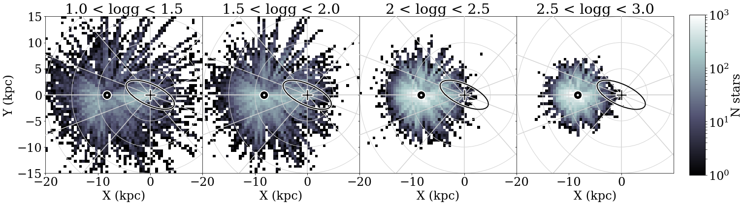
Neural network-derived ages like distmass heavily rely on the accuracy of the training set labels which transfer to the model. Small changes the training set can result in differences in the derived ages of the full training set, which contributes to the large uncertainty values around stellar ages.
The distmass catalog publishes results from six different neural network models. All six models were trained using the same subset of stars and the same ASPCAP parameters as training labels, with the only difference being the choice of APOKASC asteroseismic masses used in the training set. The APOKASC catalog publishes asteroseismic results from three different groups (initials “SS”, “MO” and “TW” - see Pinsonneault et al. 2023 in prep. for details), referred to as the “uncorrected” masses. Each set of masses also has a “corrected” counterpart, using Gaia parallaxes to calibrate the stellar radius derived from asteroseismology (e.g., Zinn et al., 2019). The calibrations are dependent on stellar and are less reliable for stars , which is why we elect to use the uncalibrated age set for our final results. Stone-Martinez et al. 2023 in prep. goes into more detail on this motivation.
Figure A.2 compares different three different age catalogs - the uncalibrated distmass ages used in this paper (green points), its calibrated counterpart (blue points), and the astroNN APOGEE VAC (Leung & Bovy, 2018; Mackereth et al., 2019) (red points) - against the APOKASC derived stellar ages on the x-axis for the subset of stars in the distmass training set. The comparison is divided by ranges in stellar (columns, increasing left to right). We find that all three catalogs suffer a “compression” in ages compared to the APOKASC values, with young stars tend to be assigned ages that are too old, and old stars tend to be fit too young. All three sets of ages predict the ages of higher with better accuracy and less scatter. For lower stars, the calibrated distmass ages predict the young ages slightly better, but and astroNN and the uncalibrated distmass predicts the older ages better. For higher stars, astroNN predicts the young ages slightly better, and distmass predicts the older ages better. This offset is thought to be caused by scatter within the training set that the neural network learns from. The asteroseismic masses are more uncertain for low stars, which results in a larger mismatch between the APOKASC results and the neural network results. The neural network essentially fits for the relation between [C/N] abundance and stellar age, which should be consistent across a broad range of . Therefore, we emphasize for low stars, the neural network likely fits more precise ages than available in the pure asteroseismology results used in the training set.
Although the age estimates show less scatter for higher stars, redefining our sample would severely limit the spatial range of the Galaxy we can access. Figure A.3 shows the face-on distribution of stars in the disk for various limits. Above , the outer disk ( kpc) and the inner disk ( kpc) disappear from the sample.
Nevertheless, we did test how redefining the sample may influence our results. In general, the observed trends and resulting conclusions do not change, motivating the use of the original sample for the increased spatial range. The radial metallicity gradient as a function of age (Figure 17) differs by less than dex kpc-1, and the radial age gradient (Figure 20) differs by Gyr kpc-1 using the higher sample.
A.3 Alpha-Age relation for different catalogs
To demonstrate how a different selection of age catalog may influence our results, Figure A.4 shows a recreation of Figure 25 for three different age samples:
-
•
Test Sample A ( range): restricting to : defining a new sample with higher surface gravity
-
•
Test Sample B (alternate distmass ages): using the Gaia-corrected APOKASC ages training set from distmass, with the original sample of .
-
•
Test Sample C (alternate astroNN ages): using astroNN ages instead of the distmass catalog, with the original sample of .
Test Sample A (Figure A.4.b) changes our limits to , shifting our sample to a different range where the age estimates are expected to be more reliable, while purposely avoiding the red clump. However, this suffers from the previously-shown lack of spatial distribution, with significantly fewer stars beyond kpc and within kpc than the original sample used in this paper. This test sample does include a larger number of stars near the solar neighborhood, however. The general location and trends across galactic location are similar, but this sample has more scatter which leads to larger contour shapes. The bimodality within the low- sequence (possible evidence for a “third infall”) around kpc is not obvious in this sample, although is perhaps present at shorter radii ( kpc).
Test Sample B uses the distmass ages using the calibrated ASPCAP training set. The Gaia-motivated calibration is dependent on (e.g., Zinn et al., 2019, Pinsonneault et al. 2023 in prep.), which results in lower stars assigned younger ages in the calibrated catalog and higher stars being assigned systematically older ages and resulting in an overall age compression in the sample obvious is Figure A.4.c. Otherwise, the results are generally similar, with the possible bimodality within the low- sequence at kpc still present in this sample. The high- sequence has more spread in age, possible due to the calibrations propagating uncertainties in the adopted calibrations (from the assumptions for example) through into the final age estimates.
Test Sample C uses astroNN ages instead of distmass in Figure A.4.d, which makes obvious the overall “compression” of the ages caused by the systematics discussed earlier; astroNN ages do not go as old or as young as the distmass ages. The general shapes and trends across the Galaxy otherwise stay the same, and the bimodality within the low- sequence is not obvious in this sample either.
We also include a reproduction of the median radial age profile (Figure 20) and the age-metallicity relation (Figure 23) using the higher- Test Sample A in Figures A.5 through A.6. As before, the trends in each plot are similar to their low- counterparts, but with higher scatter, as the range of Galaxy covered by the sample is more limited despite the lower uncertainties in stellar ages.
A.4 Summary of Age Caveats
Stellar ages are one of the most powerful quantities available in modern astronomy for revealing the history of the Milky Way, but remain challenging to measure robustly. In this study and others, it is important to consider age-related results with caution and understand the subsequent effects that changes in stellar ages may have on the conclusions. While different age catalogs show generally similar trends for the results of this paper, the quantitative aspects can differ significantly and should be regarded with healthy skepticism until more precise age estimates are available for large samples of stars.
(a) Same as Figure 25, reproduced here for ease of comparison.
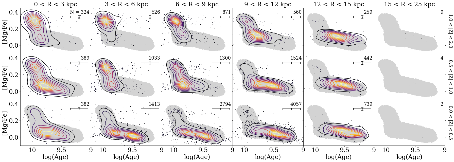
(b) Same as (a), but for a sample covering a higher surface gravity range of (Test Sample A)

(c) Same as (a), but using the “calibrated” ages from distmass trained on the Gaia-corrected APOKASC catalog (Test Sample B).

(d) Same as (a), but using stellar ages from the astroNN catalog (Test Sample C).
(a) Same as Figure 20, reproduced here for ease of comparison.

(b) Same as (a), but using a sample covering a higher surface gravity range of (Test Sample A)
(a) Same as Figure 23, reproduced here for ease of comparison.

(b) Same as (a), but for a sample covering a higher surface gravity range of (Test Sample A)