A Systematic Survey of General Sparse Matrix-Matrix Multiplication
Abstract.
General Sparse Matrix-Matrix Multiplication (SpGEMM) has attracted much attention from researchers in graph analyzing, scientific computing, and deep learning. Many optimization techniques have been developed for different applications and computing architectures over the past decades. The objective of this article is to provide a structured and comprehensive overview of the researches on SpGEMM. Existing researches have been grouped into different categories based on target architectures and design choices. Covered topics include typical applications, compression formats, general formulations, key problems and techniques, architecture-oriented optimizations, and programming models. The rationales of different algorithms are analyzed and summarized. This survey sufficiently reveals the latest progress of SpGEMM research to 2021. Moreover, a thorough performance comparison of existing implementations is presented. Based on our findings, we highlight future research directions, which encourage better design and implementations in later studies.
1. Introduction
SpGEMM is a special case of general matrix multiplication (GEMM) when two input matrices are sparse matrices. It is a fundamental and expensive computational kernel in numerous scientific computing applications and graph algorithms, such as algebraic multigrid solvers (Bell et al., 2012)(Ballard et al., 2016b), triangle counting (Davis, 2018)(Cohen, 2009)(Wolf et al., 2017)(Azad et al., 2015), multi-source breadth-first searching (Gilbert et al., 2006)(Then et al., 2014)(Buluç and Gilbert, 2011), the shortest path finding (Chan, 2007), colored intersecting (Kaplan et al., 2006)(Deveci et al., 2016), and subgraphs matching (Vassilevska et al., 2006)(Buluç and Madduri, 2011). Hence, the optimization of SpGEMM has the potential to impact a wide variety of applications.
To the best of our knowledge, this is the first survey paper that overviews the developments of SpGEMM over the past decades. The goal of this survey is to present a working knowledge of the underlying theory and practice of SpGEMM for solving large-scale scientific problems, and provide an overview of the algorithms, data structures, and libraries available. This survey covers the sparse formats, application domains, challenging problems, architecture-oriented optimization techniques, and performance evaluation of available implementations. This study follows the guidelines of the systematic literature review proposed by Kitchenham (Kitchenham, 2004), which was initially used in medical science but later gained interest in other fields as well. According to the three main phases: planning, conducting, and reporting, we have formulated the following research questions:
RQ1: What are the applications of SpGEMM, and how are they formulated?
RQ2: What is the current status of SpGEMM research?
RQ3: How do the state-of-the-art SpGEMM implementations perform?
RQ4: What challenges could be inferred from the current research effort?
Regarding RQ1, this study presents a detailed introduction to three typical applications and addresses how SpGEMM is used in these applications. This will give an insight into the requirements of SpGEMM in solving real problems. In RQ2, the study looks at existing techniques that were proposed in recent decades from different angles. Regarding RQ3, we perform some performance evaluations to have a general idea about the performance of these implementations on prevailing hardware platforms. Finally, in RQ4, we summarize the challenges and future research directions according to our investigative results.

To have a broad coverage, we perform a systematic literature survey by indexing papers from several popular digital libraries (IEEE Explore Digital Library, ACM Digital Library, Elsevier ScienceDirect, Springer Digital Library, Google Scholar, Web of Science, DBLP, arXiv) using the keywords ”SpGEMM”, ”sparse matrix”, ”sparse matrix multiplication”, ”sparse matrix-matrix multiplication”. It is an iterative process, and the keywords are fine-tuned according to the returned results step by step. We try to broaden the search as much as possible while maintaining a manageable result set. Then, we read the titles and abstracts of these papers and finally include 92 SpGEMM related papers, whose year distribution is presented in Figure 1. It can be seen that the articles in the past three years have shown a rapid upward trend.
It is difficult to give a sufficient and systematic taxonomy for classifying SpGEMM research because the same topic may have different understandings in different contexts, such as load balance of SpGEMM in distributed, shared-memory multicore, single GPU, multi-GPU and CPU+GPU. We select several topics that are frequently covered by existing papers, and present the correlation between papers and topics in table or figure of each section.
The rest of the paper is organized as follows. Section 2 introduces background in detail, including symbol notation used in this paper, some popular and state-of-the-art compression formats for sparse matrix, and several classical applications of SpGEMM. Four different SpGEMM formulations are introduced in Section 3. In Section 4, the discussion about the existing solutions for three pivotal problems of SpGEMM computation is presented. In Section 5, architecture-oriented SpGEMM optimization is introduced. Section 6 gives a comprehensive introduction to the SpGEMM optimization using different programming models. Besides, we conduct a performance evaluation covering most SpGEMM implementations in Section 7. A discussion about the challenges and future work of SpGEMM is presented in Section 8, and followed by our conclusion in Section 9.
2. Background
2.1. Preliminaries
2.1.1. Notation
In this section, we first give the symbolic representation commonly used in this paper, which is presented in Table 1. We use bold capital italic for matrices, lowercase bold italic for vectors, and lowercase italic for scalars.
| Symbol | Description | Symbol | Description |
| and are input matrices, is the output matrix | Inner product of two vectors | ||
| The -th row of | Outer product of two vectors | ||
| The -th column of | General matrix multiplication of two matrices or a matrix and a vector | ||
| The entry in the -th row and the -th column of | Multiplication of two scalars or a scalar and a vector | ||
| Dimensions: , , | Element-wise multiplication |
2.1.2. Sparse Matrix
There is no strict and formal definition of sparse matrix. The most popular one is given by Wilkinson: sparse matrix is any matrix with enough zeros that it pays to take advantage of them (Gilbert et al., 1992). Another common quantitative definition is given by Barbieri et al. (Filippone et al., 2017), that is, a matrix is sparse if its number of non-zero entries (referred to as NNZ) is .
| Format | Contribution |
| COO | (Demirci and Aykanat, 2020b)(Gremse et al., 2015)(Matam et al., 2012)(Chen et al., 2019)(Zhang et al., 2020)(Ramanathan et al., 2021)(Ramanathan et al., 2020)(Liu et al., 2021) |
| CSR | (Gustavson, 1978)(Cohen, 1998)(Buluç and Gilbert, 2008a)(Siegel et al., 2010)(Demouth, 2012)(Matam et al., 2012)(Liu and Vinter, 2014)(Patwary et al., 2015)(Liu and Vinter, 2015)(Dalton et al., 2015)(Kurt et al., 2017)(Nagasaka et al., 2017)(Elliott and Siefert, 2018)(Zhang et al., 2019)(Liu et al., 2019)(Winter et al., 2019)(Wang et al., 2019)(Li et al., 2019)(Chen et al., 2019)(Nagasaka et al., 2019) (Zhang et al., 2020)(Lee et al., 2020)(Chen et al., 2020)(Ishiguro et al., 2020)(Parger et al., 2020)(Haghi et al., 2020)(Zachariadis et al., 2020)(Rolinger et al., 2021)(Shivdikar, 2021)(Zhang et al., 2021)(Hussain et al., 2021)(Xia et al., 2021)(Rajamanickam et al., 2021) |
| CSC | (Cohen, 1998)(Zhang et al., 2021)(Zachariadis et al., 2020)(Rasouli et al., 2021)(Chen et al., 2019)(Lee et al., 2020) |
| DCSC | (Buluç and Gilbert, 2008a)(Buluç and Gilbert, 2008b)(Buluç and Gilbert, 2010)(Buluç and Gilbert, 2011)(Buluç and Gilbert, 2012)(Patwary et al., 2015)(Azad et al., 2016)(Selvitopi et al., 2020b) |
| Others | DIA(Matam et al., 2012),ELL(Ishiguro et al., 2020)(Chen et al., 2019),DCSR(Buluç and Gilbert, 2008b),BCSR(Borstnik et al., 2014),HNI(Park et al., 2022),CFM(Xie and Liang, 2019),Bitmap/BitMask(Gondimalla et al., 2019)(Kanellopoulos et al., 2019) (Pentecost et al., 2019)(Zachariadis et al., 2020)(Qin et al., 2020),RLC(Han et al., 2016)(Chen et al., 2017),RIR(Soltaniyeh et al., 2020),C2SR(Srivastava et al., 2020),Tiled structure(Niu et al., 2022) |
2.1.3. Compression Format
Storing matrices with a dense pattern often leads to a lot of useless calculations and redundant storage, because they usually have a few non-zero entries (referred to as non-zeros). The prevailing solution is to store each sparse matrix with a compression format. Table 2 summarizes the contributions using different formats.
COO, CSR, CSC, ELL, and DIA are five basic and popular compression formats. COO is the plainest format and stores the row index, column index, and value of each non-zero entry in three separate arrays. CSR is the most extensively used format in existing work. Instead of storing row indices, CSR stores the row pointers to the first non-zero entry per row. CSC replaces the column indices array of COO with column pointers. ELL compacts all non-zeros to the left side. DIA is specifically designed for diagonal sparse matrices. It stores non-zeros in each diagonal and the offset of each diagonal from the main diagonal.
In addition to the above five basic formats, some new sparse formats have been proposed over the past years. Buluç et al. (Buluç and Gilbert, 2008b)(Buluç and Gilbert, 2008a) propose double compressed sparse column (DCSC), an improved format based on CSC. It is designed for hypersparse matrix by removing all the repetitions in column pointers array. They also present DCSR format (Buluç and Gilbert, 2008b), which is a row-based dialect of DCSC. Bortnik et al. (Borstnik et al., 2014) design an efficient distributed sparse matrix multiplication algorithm using blocked CSR (BCSR) format. Park et al. (Park et al., 2022) propose huffman-coded non-zero indication (HNI) format, which is a bitmap-based data encoding. It uses non-zero indication bit-stream to replace row and column indices and encodes the stream with Huffman coding. Xie et al. (Xie and Liang, 2019) design compressed feature map (CFM) for efficiently storing sparse feature maps in convolution neural network (CNN). In SparTen proposed by Gondimalla et al. (Gondimalla et al., 2019), a sparse tensor is encoded into a two tuple of a bit-mask representation and a set of non-zeros. The bit-mask representation has 1’s for positions with non-zeros and 0’s otherwise. This bit-mask based compression idea is also used in (Kanellopoulos et al., 2019)(Pentecost et al., 2019)(Zachariadis et al., 2020)(Qin et al., 2020). Han et al. (Han et al., 2016)(Chen et al., 2017) use a CSR variation, run-length encoding (RLE), to store a sparse weight matrix in deep neural network (DNN). The new format stores a vector and an equal-size vector for each column in the weight matrix, where saves the non-zero weights, and stores the number of zeros before the corresponding entry in . Soltaniyeh et al. (Soltaniyeh et al., 2020) propose REAP intermediate Representation (RIP) to increase the throughput on FPGAs. It has three parts: shared feature, metadata and distinct features. To overcome the inefficient memory access of CSR, Srivastava et al. (Srivastava et al., 2020) propose a channel cyclic sparse row (C2SR) format, which assigns each matrix row to a fixed channel in a cyclic manner. In TileSpGEMM, Yu et al. (Niu et al., 2022) propose a sparse tile data structure which describes a sparse matrix using two levels of tile information.
2.2. Typical Applications
SpGEMM is a basic and critical component in many applications. We introduce the background of some applications and how the SpGEMM is formulated and used in these applications as follows.
2.2.1. Multi-source BFS
Breadth-first search (BFS) is a key and fundamental subroutine in many graph analysis algorithms. The goal of the BFS is to traverse a graph from a given source vertex, which can be performed by a sparse matrix-vector multiplication (SpMV) between the adjacency matrix of a graph and a sparse vector representing the source vertex (Zhang et al., 2011). Assume , then the size of is . Let be a sparse vector with and all other entries being zero, then the 1-hop vertexes from source vertex , denoted as , can be derived by the SpMV operation: . Repeating the operation from , we can receive the 2-hop vertexes from . Finally, a complete BFS for the graph from vertex is yielded (Gilbert et al., 2006). In contrast, Multi-Source BFS (MS-BFS) runs multiple independent BFSs concurrently on the same graph from multiple source vertexes, which can be formulated as SpGEMM. A simple example for MS-BFS is presented in Figure 2. Let be two source vertexes, is the adjacency matrix of the graph, and is a rectangular matrix representing the source vertexes, where and are two sparse column vectors with and respectively and all other entries being zero. Then, the sparse matrix representing the 1-hop vertexes (denoted as ) from source vertexes is give by . Repeat the multiplication of adjacency matrix and : , we can derive the 2-hop vertexes from . Finally, we get the results of BFS from vertices 1 and 2, which are and respectively.
Many applications run hundreds of BFSs over the same graph. Compared with running BFSs sequentially, running multiple BFSs concurrently in a single kernel allows us to share the computation between different BFSs without paying the synchronization cost (Gilbert et al., 2006). As one of the most expensive operations of MS-BFS, SpGEMM is worthy of more attention to be paid.

2.2.2. Markov Clustering (MCL)
Clustering is one of the unsupervised learning methods for statistical data analysis, and MCL is one of the graph clustering algorithms proposed for biological data (Selvitopi et al., 2020b). Using MCL, the closely connected points are grouped into clusters by performing random walks on a graph based on Markov chains. Let denote a probability matrix, and each entry in the matrix is the probability of each point reaching others. The sum of each column in this matrix is 1. There are three steps in the clustering iteration. In the first step of expansion, the probability matrix of reaching other points starting from any point after one step is given by . This not only strengthens the connection between different areas, but also leads to the convergence of probabilities. In the second step, all entries smaller than a given threshold are pruned. Then, the third step of inflation is required to weaken the possibility of loosely connected points by computing the power of each element in the probability matrix. Next, the matrix is replaced with the new matrix and used for next iterations. After a number of iterations, the points in a graph are gradually clustered into groups.
Due to the high time and memory overhead of MCL, high performance MCL (HipMCL) algorithm is proposed for fast clustering of large-scale networks on distributed platforms (Selvitopi et al., 2020b).
2.2.3. Algebraic Multigrid Solvers
Algebraic Multigrid (AMG) is a multi-grid method developed based on Geometric multigrid (GMG). AMG iteratively solves large and sparse linear system by automatically constructing a hierarchy of grids and inter-grid transfer operators (Falgout, 2006)(Briggs et al., 2000). Generally, AMG includes two processes: setup and solve. The setup phase constructs multiple components of multigrid algorithm. The solve phase executes multigrid cycling based on these components, and SpMV dominates this phase. SpGEMM is an important kernel in setup phase, whose critical steps are presented in Algorithm 1. It first constructs interpolation operator based on input matrix (line 3), then the restriction operator is the transposition of (line 4). Finally, the coarse-grid system is constructed using Galerkin product (line 5), which is implemented with two SpGEMMs (Bell et al., 2012)(Ballard et al., 2016b). Generally, is tall and skinny, and is short and fat. Their non-zeros’ distribution is closely related to the used interpolation algorithms.
These SpGEMMs, taking more than of the total construction time, are the most expensive components. Moreover, the construction of operators (thus SpGEMM) is an expensive part in overall execution since it may occur at every time step (for transient problems) or even multiple times per time step (for non-linear problems), making it important to optimize SpGEMM (Elliott and Siefert, 2018).
2.2.4. Others
SpGEMM is also one of the most important components for genome assembly (Selvitopi et al., 2020a)(Guidi et al., 2021a)(Guidi et al., 2021b), NoSQL database (Cohen et al., 2009)(Gadepally et al., 2015)(Hutchison et al., 2015), triangle counting (Cohen, 2009)(Wolf et al., 2015)(Wolf et al., 2017), graph contraction (Gilbert et al., 2008), graph coloring (Kaplan et al., 2006)(Deveci et al., 2016), the all pairs shortest path (Chan, 2007), sub-graph (Vassilevska et al., 2006)(Buluç and Madduri, 2011), cycle detection or counting (Censor-Hillel et al., 2015), and molecular dynamics (Weber et al., 2015)(Akbudak and Aykanat, 2014).
3. Formulations
3.1. Overview
| Formulation | Contribution |
| Row-by-row | (Gustavson, 1978)(Siegel et al., 2010)(Matam et al., 2012)(Liu and Vinter, 2014)(Liu and Vinter, 2015)(Patwary et al., 2015)(Dalton et al., 2015)(Ballard et al., 2016b)(Nagasaka et al., 2017)(Deveci et al., 2017)(Akbudak et al., 2018)(Demouth, 2012)(Deveci et al., 2018b)(Deveci et al., 2018a)(Elliott and Siefert, 2018)(Nagasaka et al., 2019)(Zhang et al., 2019)(Chen et al., 2019)(Liu et al., 2019) (Winter et al., 2019)(Li et al., 2019)(Soltaniyeh et al., 2020)(Haghi et al., 2020)(Chen et al., 2020)(Srivastava et al., 2020)(Demirci and Aykanat, 2020a)(Shivdikar, 2021)(Zhang et al., 2021)(Hussain et al., 2021)(Rajamanickam et al., 2021)(Demirci and Aykanat, 2020b)(Niu et al., 2022) |
| Inner-product | (Borstnik et al., 2014)(Zachariadis et al., 2020)(Azad et al., 2015)(Xie and Liang, 2019)(Selvitopi et al., 2020b)(Akbudak et al., 2018)(Akbudak and Aykanat, 2017)(Ramanathan et al., 2020) |
| Outer-product | (Cohen, 1998)(Yuster and Zwick, 2005)(Buluç and Gilbert, 2008a)(Buluç and Gilbert, 2008b)(Matam et al., 2012)(Akbudak and Aykanat, 2014)(Srikanth et al., 2020)(Gu et al., 2020)(Ballard et al., 2016b)(Akbudak et al., 2018)(Akbudak and Aykanat, 2017)(Lee et al., 2020)(Zhang et al., 2020)(Selvitopi et al., 2019) (Pal et al., 2018) |
| Column-by-column | (Buluç and Gilbert, 2008b)(Azad et al., 2016) |
In sparse matrix multiplication, two sparse matrices that are multiplied can be accessed either by row or column. This derives four SpGEMM formulations, which are row-by-row (RbR), row-by-column/inner-product (IP), column-by-row/outer-product (OP), and column-by-column (CbC). Table 3 summarizes the existing work using different SpGEMM formulations. As shown in the table, RbR is the most popular and favored formulation by researchers, followed by OP, then IP, and the least explored is CbC. In this section, we introduce the calculation of the four formulations, followed by a discussion on the advantages and disadvantages of the four formulations.
3.2. Row-by-row
RbR formulation is based on the row-wise partitioning of two input matrices. Each row of is calculated by summing the intermediate multiplication results of each non-zero entry of and corresponding row of , i.e.
| (1) |
where denotes the set of column indexes of the non-zeros in the -th row of . Figure 3(a) presents an example illustrating the computing pattern of RbR formulation.

3.3. Inner-product
This formulation is based on the row-wise and column-wise partitioning of and respectively. The result matrix consists of the inner product of each row of and each column of , i.e.
| (2) |
where denotes the set of indexes such that both the entries and are non-zero. An example that illustrates the inner-product formulation is presented in Figure 3(b).
3.4. Outer-product
This formulation is based on the column-wise and row-wise partitioning of input matrices and , respectively. The result matrix is calculated by summing the outer product of each column of and corresponding row of , i.e.
| (3) |
An example that illustrates the outer-product formulation is presented in Figure 3(c).
3.5. Column-by-column
This formulation is based on the column-wise partitioning of two matrices, which is similar to the RbR formulation. Each column of the result matrix is calculated by summing the intermediate multiplication results of each non-zero entry of and corresponding column , i.e.
| (4) |
where denotes the set of row indexes of the non-zeros in the -th column of . An example that illustrates the column-by-column is presented in Figure 3(d).
3.6. Discussion
Srivastava et. al (Srivastava et al., 2020) compare the data reuse and on-chip memory requirement of four SpGEMM formulations. In their work, data reuse is defined as the ratio of the number of multiply-accumulate (MAC) performed to the size of data read from or written to memory. They assume that all three sparse matrices are square () and have the uniform non-zero distribution, and and have the same number of non-zero entries (). Assuming that the NNZ of , and , has a small difference, their discussion can be concluded in two points. First, the relationship between the data reuse of four formulations is: . Second, for the on-chip memory, the relationship is .
Here we extend the discussion to the size of intermediate results. Let represent the NNZ in output matrix . For RbR SpGEMM, one non-zero entry of and the corresponding row of are loaded and multiplied, generating a vector of size . Therefore, its size of intermediate results that require to be reduced is . For IP SpGEMM, a dot product between one row of and one column of is performed, generating one non-zero entry of . Therefore, no intermediate results are generated. For OP SpGEMM, an outer product between one column of and one row of is performed, generating an intermediate result matrix of . Its total size of intermediate results is . CbC SpGEMM is similar to RbR SpGEMM. Therefore, the relationship between the size of intermediate results is .
Besides, the four SpGEMM formulations are different in storage format and index matching. RbR prefers to store two input matrices and the output matrix in row-major layout, such as CSR. On the contrary, the column-major layout, such as CSC, is preferred by CbC. However, IP prefers to store two input matrices in row-major and column-major layouts, respectively. OP prefers to an opposite storage format. There is no preference for how the resulting matrix is stored for IP and OP. Among the four SpGEMM formulations, only IP requires index matching.
Generally, the two most basic operations of SpGEMM are scalar multiplication and addition. However, they can also be customized and redefined in some applications. For example, Selvitopi et al. (Selvitopi et al., 2020a) and Guidi et al. (Guidi et al., 2021b) present a custom semiring to overload multiplication and addition of SpGEMM in a similar protein sequences identification algorithm. Some popular libraries, such as CombBLAS (Azad et al., 2022), CTF (Solomonik et al., 2014), and GraphBLAS (Davis, 2019), support user-defined multiplication and addition on semirings. On that account, SpGEMM can be generalized and extended to more fields.
4. Key Problems and Techniques
4.1. Overview
The typical workflow of SpGEMM is presented in Figure 4, which has five stages, including size prediction, memory allocation, work partition and load balance, numeric multiplication, and result accumulation. The size prediction stage aims to predict the memory footprint of result matrix before real execution. The memory allocation stage allocates memory space for result matrix on target device. The objective of the work partition and load balance stage is to design an efficient algorithm to fully exploit the performance of parallel processors. Numeric multiplications and partial additions are performed, and a large number of intermediate results are also generated in this stage. Result accumulation desires to reduce these results and calculate final results.

The multiplication result of two sparse matrices is also a sparse matrix, which requires to be stored in a compression format. In CSR/CSC format, NNZ of a sparse matrix dominates its memory footprint, and the sparsity of the result matrix is always unknown in advance. However, precise prediction for the size of result matrix is always expensive in practice. Moreover, with the popularization of multi/many-core processors and distributed systems, the parallelization of intensive computing has become a necessary step for accelerating applications. SpGEMM involves three sparse matrices, which significantly increases the complexity of the problem. Last but not least, due to the sparsity and irregular non-zero distribution, designing an efficient accumulator (the data structure that we use to hold the intermediate results) is also a challenging task.
In the following sections, we discuss in detail the approaches to deal with three challenging problems: size prediction, work partition and load balance, and result accumulation.
4.2. Size Prediction
4.2.1. Precise Prediction
SpGEMM algorithms using precise prediction usually consist of two phases: symbolic and numeric phases. In the symbolic phase, the precise NNZ in each row/column of the output matrix is computed based on row and column indices of input sparse matrices, an example is shown in Figure 5. Real values of non-zeros are calculated in the numeric phase.

The implementations of SpGEMM in Kokkos Kernels (Rajamanickam et al., 2021), cuSPARSE (NVIDIA, 2021), MKL (Intel, 2021), and RMerge (Gremse et al., 2015) are typical representatives of this method. Besides, existing work (Demouth, 2012), (Nagasaka et al., 2017), (Demirci and Aykanat, 2020b) and (Akbudak and Aykanat, 2014) also exploit this approach. In order to speed up the symbolic phase, Deveci et al. (Deveci et al., 2017)(Deveci et al., 2018b) design a graph compression technique to compress the matrix by packing its columns as bits. In (Gu et al., 2020), the authors estimate the memory requirement for as well as the number of bins and allocate space for global bins in the symbolic phase. SpECK (Parger et al., 2020) uses size information collected in symbolic execution to guide the selection of accumulators in numeric phase.

4.2.2. Probabilistic Method
Cohen (Cohen, 1997) transforms the problem of estimating NNZ in the output matrix to the size estimation of reachability sets in a directed graph, and presents a Monte Carlo-based algorithm to estimate the size of reachability sets. The algorithm can be demonstrated using a hierarchical structure graph of matrix product, as shown in Figure 6. The algorithm starts by assigning a vector of same size, initialized with exponential-distribution random samples, to each node in . The vector of each node in the higher layer is equal to the column-wise minimum of the vectors of its neighbors in the lower layer. Finally, NNZ in each row of is estimated based on the vector of each node in . For any tolerated relative error , it can compute an approximation of NNZ in result matrix in time . Then, Amossen et al. (Amossen et al., 2014) improve this method to expected time for some particular . Anh et al. (Anh et al., 2016) utilize a similar size estimation technology based on the rows sampling of and . In (Cohen, 1997), the authors introduce an algorithm to determine the multiplication order of chain products with minimal number of calculation operations. Paper (Selvitopi et al., 2019) also uses this three-layer graph representation to estimate the size of result matrix.
4.2.3. Upper-Bound Prediction
The third method computes an upper-bound NNZ in the output matrix and allocates corresponding memory space. The most commonly used method is to count NNZ in the corresponding rows of for each non-zero entry in . Taking the matrices presented in Figure 5 for example, the upper bound of NNZ in each row of the output matrix is stored in the array . The first row of has two non-zeros, whose column indices are 2 and 4. Therefore, the upper-bound NNZ in the first row of equals to the sum of NNZ in the second and forth rows of . The ESC algorithm (Bell et al., 2012)(Dalton et al., 2014) proposed by Bell et al. is a representative of this method. Nagasaka et al. (Nagasaka et al., 2019) also count a maximum of scalar non-zero multiplications per row of the result matrix. Then each thread allocates a hash table based on the maximum and reuses the hash table throughout the computation by re-initializing at the beginning of calculating each row.
4.2.4. Progressive Method
The fourth method, also known as the progressive method, dynamically allocates memory as needed. It first allocates memory of proper size and then starts matrix multiplication. A larger memory block is re-allocated if the current memory is insufficient. The implementation of SpGEMM in Matlab (Gilbert et al., 1992) is a representative of this method. It first guesses the size, and then allocates a memory block that is larger by a constant factor (typically 1.5) than the current space if more space is required at some point.
Liu and Vinter (Liu and Vinter, 2014)(Liu and Vinter, 2015) propose a hybrid method which calculates the upper-bound NNZ for each row and groups all rows into multiple bins according to NNZ. The method allocates space of the upper-bound size for short rows and progressively allocates space for long rows. In TileSpGEMM proposed by Yu et al. (Niu et al., 2022), it first calls the symbolic implementation in NSparse (Nagasaka et al., 2017) to get the sparse tile structure of . Then, it uses binary search to find intersection sparse tiles from and . Finally, bit mask operations are used to calculate the number of non-zeros of each tile in .
4.2.5. Discussion
Of the four methods, precise method not only saves the memory usage, but also enables the sparse structure of to be reused for different multiplies with the same structure of input matrices (Deveci et al., 2018b)(Gustavson, 1978). Moreover, it presents significant benefits in graph analytics, because most of them work only on the symbolic structure, no numeric phase (Wolf et al., 2017). However, the calculation of two phases means that it needs to iterate through the input matrices twice, leading to higher computation overhead than other methods. The accuracy and the speed of the second method depend on the probabilistic algorithm used, and additional memory allocation must be launched when the estimate fails. The upper-bound method is efficient and easy to implement, but it usually leads to memory over-allocation. The progressive method allocates memory dynamically as needed, and additional memory allocation must also be launched when the first allocation fails. In practice, the choice needs to be made according to the discussed problems.
4.3. Work Partition and Load Balancing
The mainstream work partition and load balancing methods are presented in Figure 7, and we introduce and discuss these methods in detail in the following sections.
4.3.1. Block Partition
Block partition of SpGEMM can be categorized into 1D, 2D and 3D algorithms based on how they partition the work among computing units (Azad et al., 2016)(Ballard et al., 2016a). We first introduce the workcube notation before diving into the details, as shown in Figure 8(b). The front, top, and side views of the workcube represent the two input matrices and the output matrix presented in Figure 8(a), respectively. The workcube can be divided into voxels. Each voxel inside represents the scalar multiplication of two non-zeros, which are mapped to cells of the voxel in the front and top views, and contributes to its projection in the side view (Ballard et al., 2013). Based on this projection, task partition of SpGEMM can be seen as the partition of workcube in different dimensions. Next, we introduce 1D, 2D and 3D partition based on this notation.

1D Partition. 1D partition only divides the workcube in one of the three dimensions. As shown in Figure 9, each sub-figure represents a variant of 1D partition. A ”layer” of the workcube is assigned to one computing unit in all variations. Figure 9(a) divides the workcube by planes parallel to the top view, referred to as -partition. Each computing unit is responsible for the multiplication of a set of rows in and the entire matrix , producing the corresponding rows of . Similarly, Figures 9(b) and (c) divide the workcube by planes parallel to the front view and side view, respectively. We refer to these two partition variants as -partition and -partition.

-partition. Liu et al. (Liu and Vinter, 2014) group rows of to different bins according to their upper-bound NNZ to maintain a balanced load. Nagasaka et al. (Nagasaka et al., 2017) partition rows of according to precise NNZ in each row in numeric phase. Kurt et al. (Kurt et al., 2017) propose to assign one thread block to a fixed number of rows in and assign a same number of threads in the block to complete the row-wise multiplication of each row in and corresponding entries in . Deveci et al. (Deveci et al., 2017) propose a hierarchical and parallel SpGEMM algorithm based on Kokkos library (Edwards et al., 2014). At the first level, one kokkos-team is assigned to calculate a set of rows of . Each kokkos-thread within the team is responsible to produce a subset of these rows at the second level. Multiple vector-lanes in one kokkos-thread are assigned to perform the row-wise multiplication of each non-zero entry in the subset of and corresponding rows in at the third level. They also explore -partition but with different task assigning schemes for HPC architectures (Deveci et al., 2018b). Winter et al. (Winter et al., 2019) present a partition scheme assigning the same NNZ of to each block while ignoring the row boundaries. Instead of splitting rows evenly (Elliott and Siefert, 2018), Li et al. (Li et al., 2019) split the matrix into multiple row blocks based on NNZ. To address the input or output reuse problem, Zhang et al. (Zhang et al., 2021) split matrix into row fibers and dispatch them to processing elements (PEs) in a SpGEMM accelerator GAMMA, and each PE then performs a linear combination of row fibers of to produce a row fiber of . Shivdikar et al. (Shivdikar, 2021) group multiple rows in a single window and assign one PIUMA (Programmable Integrated Unified Memory Architecture) block to a window. The size of a window depends on the scratchpad size.
-partition. Azad et al. (Azad et al., 2015) assign processors to process columns of the upper triangular matrix in triangle counting. Lin et al. (Lin et al., 2013) design an architecture for SpGEMM on FPGAs, the computation is partitioned evenly to all PEs, and each PE is assigned to calculate multiple columns of matrix .
-partition. Based on the outer-product multiplication, Deveci et al. (Deveci et al., 2018a) divide rows of into blocks so that each block can be fitted into the HBM of KNL. This partition also induces a row-wise partition of . Zhang et al. (Zhang et al., 2020) optimize the outer-product SpGEMM by compacting non-zeros of each row in to the left so that the data locality for both input and output matrices are jointly optimized. Gu et al. (Gu et al., 2020) develop an improved ESC SpGEMM based on outer product. They group the expanded triples into bins to saturate memory bandwidth.
Others. Ballard et al. (Ballard et al., 2016b) present a theoretical and detailed analysis for the communication cost of Galerkin triple product in the smoothed aggregation of AMG methods. They conclude that the row-by-row product (-partition) is the best 1D method for the first two multiplications, and the outer product (-partition) is the best 1D method for the third multiplication.
Most of SpGEMM can be implemented using 1D partition. However, when the NNZ in columns or rows of the matrix or increases, the communication overhead becomes substantially huge in distributed computing. This indicates that a ”layer” in 1D partition is required to be processed by more computing units. Therefore, the 2D algorithms with fine-grained partition are proposed.
2D Partition. 2D algorithms divide the workcube in two of the three dimensions, so there are also three variants. Figure 10(a) illustrates three partition variants that divide the workcube by planes parallel to two of the three views (top and front views, front and side views, top and side views), referred to as -partition, -partition and -partition hereafter. In -partition, each computing unit computes a block of . However, in -partition and -partition, each computing unit computes a block of intermediate results of .

-partition. SpSUMMA was first proposed by Buluç et al. (Buluç and Gilbert, 2008b)(Buluç and Gilbert, 2008a) based on dense SUMMA algorithm (van de Geijn and Watts, 1997). They also present a comparative SpCannon algorithm based on dense Cannon algorithm (Cannon, 1969). Both algorithms logically organize processors as a 2D grid, and map a block of and to each processor. In SpSUMMA, each processor broadcasts data to other processors in the same row/column of the grid, and also receives data broadcast by these processors. In SpCannon, processors exchange data using point-to-point communication. In both algorithms, each processor accesses a row block of and column block of , and calculates a result block of , which conforms with -partition. Matrix partition similar to SUMMA is also used by Jin et al. (Jin and Ziavras, 2004). Patwary et al. (Patwary et al., 2015) partition by row, while partition by column when a certain condition is satisfied.
-partition. Deveci et al. (Deveci et al., 2018a) partition and by row for GPU. When one partition of cannot fit in GPU fast memory, column-wise partition is applied for row strip of .
2D algorithms perform reasonably well on a few hundred processes. However, as the number of processes increases, the communication cost becomes a bottleneck, and 3D algorithms were developed to reduce the communication cost.
3D Partition. 3D algorithms divide all three dimensions of the workcube. As shown in Figure 10(b), each computing unit owns a block of and a block of to compute an intermediate result block of the matrix .
Azad et al. (Azad et al., 2016) present a parallel implementation of the 3D SpGEMM algorithm. Hussain et al. (Hussain et al., 2021) use a similar 3D partition, while dividing each block of into multiple batches to meet the size of available memory. To avoid excessive communications and logistic operations of 2D SpSUMMA, Weber et al. (Weber et al., 2015) propose a novel SpGEMM algorithm MPSM3 for the computation of the density matrix in electronic structure theory. All processes are organized as a 3D Cartesian topology, and each box in the workcube is assigned to a specific process on terms of the physical properties of the problem. Yu et al. (Niu et al., 2022) divide two input sparse matrices into a number of 16-by-16 tiles to utilize 8-bit unsigned char data type for local indices.
4.3.2. Graph Partition
Traditional block-based matrix partitions rarely consider the workload (NNZ in each block) assigned to each processing element. For example, SpSUMMA presumes that non-zeros are uniformly and randomly distributed across the row/column, which may not hold for most sparse matrices.
Hypergraph Partition. The hypergraph representation for , denoted as , is defined as a set of vertices and a set of nets (hyperedges) . Here we take the outer-product SpGEMM as an example to introduce the hypergraph based partition. In , each vertex in denotes the outer product of the column of with the row of . contains a vertex for each non-zero entry in . contains a net for each non-zero entry in . Figure 11(a) shows an example of SpGEMM and Figure 11 (b) shows its hypergraph representation. The task of hypergraph partitioning is to divide a hypergraph into two or more roughly equal-sized parts such that a cost function on the nets connecting vertices in different parts is minimized (Çatalyürek et al., 2011).

Bipartite Graph Partition. A bipartite graph for , denoted as , is defined as two disjoint sets of vertices and , and a set of edges . Also take outer-product SpGEMM as an example. The semantics of each vertex in is the same with those in . The difference is that the dependence of is captured with edges, instead of a net. If an outer product represented by produces a partial result for , an edge connecting vertices and is added in . An example of a bipartite graph for the outer-product SpGEMM is presented in Figure 11(c).
Hypergraph-based partition was first applied in outer-product SpGEMM by Akbudak et al. (Akbudak and Aykanat, 2014). Besides, they also present two extended hypergraph model, which partitions the matrix by row and column, respectively. Ballard et al. (Ballard et al., 2016a) present a fine-grained hypergraph model, in which each vertex is either a scalar multiplication or a non-zero entry. Based on this hypergraph model, Kurt et al. (Kurt et al., 2017) use an iterative method to construct hypergraph partitions to ensure that the data entries involved in each partition does not exceed the cache capacity. Akbudak et al. (Akbudak and Aykanat, 2017) use hypergraph model to improve outer-product and inner-product SpGEMM.
Akbudak et al. (Akbudak et al., 2018) propose and compare multiple computational partitioning models based on hypergraph and bipartite graph partitioning, with the aim of reducing message volume. Further, three communication hypergraph partitioning models for three SpGEMM formulations are proposed to reduce the latency cost. The bipartite graph model for row-by-row SpGEMM was later used by Demirci et al. (Demirci and Aykanat, 2020b). Instead of associating two weights with each vertex, they propose a three-constrained partitioning in which each vertex is associated with three weights. Selvitopi et al. (Selvitopi et al., 2019) apply bipartite graph and hypergraph models for simultaneous scheduling of the map and reduce tasks for MapReduce jobs. Demirci et al. (Demirci and Aykanat, 2020a) propose hypergraph models for 2D and 3D partitioning to improve the performance of 2D and 3D SpGEMM.
4.3.3. Discussion
Each partition algorithm usually has its own design considerations and advantages. As the most commonly used sparse formats, CSR and CSC usually store sparse matrices by rows and columns, respectively. It is compatible with the 1D partition. The workload of 1D partition is closely related to the non-zeros distributions in the divided rows or columns, and the non-zeros distributions in the other sparse matrix. Taking -partition for example, we assume that each thread or a group of threads are responsible for the multiplication of one row of and entire . If is a regular sparse matrix and has uniform non-zeros distribution, then the NNZ in each row of determines the workload of each computing unit. Therefore, the longest row of dominates the performance. The problem of load imbalance is more serious and complicated if is irregular. 2D and 3D partitions are fine-grained and produce a more balanced workload than the 1D partition. Communication cost is an important metric for the distributed system. In the 1D partition, each work process accesses an entire input matrix ( for -partition, for -partition) or output matrix ( for -partition), which requires a huge communication overhead. Differently, 2D and 3D partitions just access some rows/columns, or partial non-zeros. The graph partitioning algorithms build computation and communication graph models to ensure load balance and minimum communication cost. For SpGEMM with an irregular computation pattern, graph partitioning algorithms achieve a more balanced load and lower communication cost than block partitioning algorithms, but at the cost of higher partitioning overhead.
4.4. Result Accumulating
According to the storage structure of the intermediate results, we classify accumulators into three types: dense, sparse, and hybrid accumulators. The related researches are shown in Figure 12.
4.4.1. Dense Accumulator
Dense accumulators use dense vectors to cache the intermediate results of current ”active” columns or rows in the result matrix. The most popular dense accumulator, was first proposed by Gustavson (Gustavson, 1978), usually has three vectors. The first one stores real values. The second one is used as a tag array to check if a column index has been inserted before. The third one stores column indexes. An example of the dense accumulator is presented in Figure 13.

Gustavson’s algorithm allows random access to a single entry in a specified time, and it is widely used and improved by many successive researches (Gilbert et al., 1992)(Patwary et al., 2015)(Siegel et al., 2010)(Lee et al., 2020). For example, the SPA accumulator in Matlab (Gilbert et al., 1992) uses a dense vector of the same size as the column size of , a dense vector with true/false ”occupied” flags, and an unordered list of the indices whose ”occupied” flags are true. Elliott et al. (Elliott and Siefert, 2018) note that prolongation matrices in the AMG method are usually tall and skinny, so they use a local dense lookup array for each thread that supports fast memory space allocation for result matrix by page-aligned and size-tracked techniques.
4.4.2. Sparse Accumulator
In sparse accumulator, intermediate results for a row are stored in compact data structures. There are two types of method for merging: list and hash-based methods.
List-based accumulating usually sorts the intermediate results by column indexes. According to the sorting algorithms utilized, we classify researches as follows. Radix sort based methods allocate the entries to be sorted to some ”buckets”, so as to achieve the goal of sorting. Bell et al. (Bell et al., 2012) propose the ESC algorithm, which sorts many scalar products in the second phase. It has been improved in (Liu and Vinter, 2015) and (Li et al., 2019). Dalton et al. (Dalton et al., 2015) use the B40C radix sort algorithm (Merrill and Grimshaw, 2011) which allows specifications in the number and location of the sorting bits to accelerate the sort operation. Gu et al. (Gu et al., 2020) use an in-place radix sort to group keys by a single byte sharing the same valid byte position. In (Liu et al., 2019), a sparse accumulator, which sorts data in the GPU registers, is proposed. Merge sort based methods first divide the sequence to be sorted into several subsequences. Then each subsequence is ordered, and all subsequences are combined into an overall ordered sequence. In (Gremse et al., 2015), the sparse rows of selected and weighted by corresponding non-zeros of , are merged in a hierarchical way similar to merge sort. Besides, Liu et al. (Liu et al., 2019) propose a GPU register-based merge algorithm, which demonstrates significant speedup over its original implementation. Heap sort based accumulator is proposed by Azad et al. (Azad et al., 2016). The intermediate result is represented as a list of triples, and each triple includes row index, column index and value of each non-zero entry. A -way merge on lists of triples is performed by maintaining a heap of size , which stores the current minimum entry in each triple list. Then a multi-way merge routine finds the minimum triple from the heap and merges it into the current result. Nagasaka et al. (Nagasaka et al., 2019) implement a heap-sort based sparse accumulator on multicore architectures.

Hash-based. Hash-based sparse accumulator first allocates a memory space based on the upper bound estimation as the hash table and uses the column indexes of the intermediate results as the key. Then the hash table is required to be shrunk to a dense state. Finally, we sort the values of each row of the result matrix according to their column indexes to obtain the final result matrix compressed with sparse format (Liu et al., 2019). An example is shown in Figure 14. SpGEMM implementation in cuSPARSE (Demouth, 2012)(NVIDIA, 2021) is a representative of this accumulator. Deveci et al. (Deveci et al., 2013) design a hashmap-based, two-level, sparse accumulator that supports parallel insertions and merges from multiple vector lanes. Weber et al. (Weber et al., 2015) use the hash table to store each row of the matrix based on the distributed BCSR format. In (Anh et al., 2016), the row and column indices of an intermediate result, normally stored in two 32-bit numbers, are first compacted into a single 32-bit value and then inserted into hash table as key. It is helpful to accelerate the later sorting operation. Nagasaka et al. (Nagasaka et al., 2017) utilize vector registers in KNL and multi-core architectures for hash probing to accelerate hash-based SpGEMM. Their hash function is defined as the reminder after division of the column index multiplied by a constant number by hash table size. Liu et al. (Liu et al., 2019) optimize the data allocations of each thread in a hash-based accumulator utilizing GPU registers. Selvitopi et al. (Selvitopi et al., 2020b) compare the heap and hash sort in distributed HipMCL, and conclude that the latter method performs better.
4.4.3. Hybrid Accumulator
Deveci et al. develop KKMEM (Deveci et al., 2017) and KKSpGEMM (Deveci et al., 2018b) algorithms, which support two hash-based accumulators and one dense accumulator. Which accumulator to use depends on the features of the discussed matrix. KKTri-Cilk algorithm (Yasar et al., 2018) uses a similar accumulator to that in the KKSpGEMM algorithm. Meanwhile, it is optimized in the Cilk implementation.
Sparse or dense accumulators are selected according to the distribution of non-zeros in different parts of a matrix. Liu et al. (Liu and Vinter, 2014)(Liu and Vinter, 2015) propose a hybrid parallel result accumulating method. Three sort-based accumulators are selected according to the upper-bound NNZ in each row. In the spECK algorithm (Parger et al., 2020), a local balancer decides which accumulator to use for each block to achieve the best expected performance from the following three accumulators: direct reference, hashing, or dense accumulation. The hash function of its hash-based accumulator multiplies the element index with a prime number and then divides the result by hash table size. TileSpGEMM (Niu et al., 2022) uses the sparse accumulator working on a sparse tile and the dense accumulator working on a dense tile. Whether a tile is dense or sparse is determined by a preseted threshold.
4.4.4. Discussion
Compared with sparse accumulators, dense accumulator requires a large memory space, especially in high concurrent scenarios. They usually require to maintain a private dense accumulator for each thread or thread group, which greatly reduces the scalability of the algorithm. There are three cases in which dense accumulators are preferred: (1) in hybrid accumulators to process the rows with a large number of non-zeros per row; (2) in SpGEMM algorithms on CPU whose large cache and modest computing cores are preferred by dense accumulator; (3) in SpGEMM whose result matrix has small column size. In contrast, the sparse accumulators have lower memory requirement and are more suitable for SpGEMM whose result matrix has a large number of columns. At the same time, sparse accumulators are also the primary choice for GPU-based SpGEMM algorithm, because GPU has limited shared memory. Among sparse accumulators, hash-based accumulators have low memory space requirement, with the cost of handling collisions. For three list-based sparse accumulators, the performance of the used sorting algorithm determines their performance. Heap and merge sort has the same time complexity, while the latter presents a higher space complexity. Radix sort is preferred when processing large-scale array.
5. Architecture Oriented Optimization
Different computer architectures usually have different computing and memory features, so the optimization of SpGEMM is closely related to the architecture used. In the following sections, we introduce SpGEMM optimization for five popular architectures: CPU, GPU, FPGA, ASIC, heterogeneous, and distributed platform. Figure 15 summarizes existing contributions on different architectures.
5.1. CPU-based Optimization
5.1.1. Optimization for Memory Access
Patwary et al. (Patwary et al., 2015) propose to divide and by row and column, respectively, aiming to alleviate the problem of high L2 cache misses caused by dense accumulator. Elliott et al. (Elliott and Siefert, 2018) present a single-phase OpenMP variant of the Gustavson algorithm. They use page-aligned allocations and track used size and capacity separately to accelerate the allocation of thread-local memories. Gu et al. (Gu et al., 2020) use the propagation block technique to improve the memory bandwidth utilization of OP SpGEMM. They first save the multiple tuples generated by the outer product into multiple partially sorted bins, and then sort and merge each bin independently. Chen et al. (Chen et al., 2019)(Chen et al., 2020) design multiple SpGEMM kernels based on different sparse formats. They all utilize coalesced DMA transmission instead of discrete memory access to achieve fast data loading from main memory. Furthermore, they reserve a minimum partition of in local data memory to improve data reuse and avoid redundant data loading.
5.1.2. Optimization for Load Balance
In (Patwary et al., 2015), matrices are divided into small partitions and dynamic load balancing is used over the partitions. They find that better results are achieved when the total number of partitions is - times the number of threads. Chen et al. (Chen et al., 2019)(Chen et al., 2020) present a three-level partitioning scheme for Sunway architecture. At the first level, each core group in the SW26010 processor performs the multiplication of a sub- and . At the second level, each CPE core in a core group multiplies the sub- by a sub-. At the third level, to fit the 64 KB local data memory in each CPE core, sub- and sub- are further partitioned into several sets. To achieve a balanced load, they divide and according to the computational loads rather than rows.
5.1.3. Optimization for Data Structure
Patwary et al. (Patwary et al., 2015) store each column partition of in an individual CSR format. This requires to change the data structure of from CSR to blocked CSR in advance, which brings a significant format conversion overhead. Therefore, they use a simple upper-bound method to estimate the proportion of non-zeros per row that exceeds the size of the L2 cache, and format conversion occurs only when this proportion is higher than 30%.
5.2. GPU-based Optimization
GPU has emerged as a promising computing device to HPC for its massive parallelism and high memory bandwidth. On the one hand, a GPU has thousands of streaming processors (SP). Application optimization on GPU should address the problem of scalable parallelism and load unbalancing. On the other hand, GPU has a hierarchical memory architecture including thousands of registers, on-chip shared memories and caches, and local and global memory. Most GPU architecture-oriented optimizations aim to reduce the memory traffic between on-chip and global memory.
5.2.1. Optimization for Memory Access
In (Dalton et al., 2015), Dalton et al. propose an improved ESC method, which stores the non-zeros of in shared memory to avoid repeated loading from global memory. In (Winter et al., 2019), Winter et al. propose an adaptive chunk-based GPU SpGEMM approach (AC-SpGEMM), which improves ESC algorithm by reducing intermediate results of within shared memory. Gremse et al. (Gremse et al., 2015) also use shared memory to merge intermediate results. The main idea is to reduce the overhead of global memory accesses by merging rows using sub-warps. Then in (Nagasaka et al., 2017), Nagasaka et al. propose a fast SpGEMM algorithm that only requires a small amount of memory and achieves high performance. Since the memory subsystems of NVIDIA GPU differ from generation to generation significantly in both bandwidth and latency, two different data placement methods are proposed in (Deveci et al., 2018a). One is to keep the partitions of and in fast memory and stream the partitions of to shared memory. The other is the opposite. Which method to choose often depends on the features of the input matrices. In (Liu and Vinter, 2014)(Liu and Vinter, 2015), memory pre-allocation for the result matrix is organized using a hybrid approach that saves a large amount of global memory space.
5.2.2. Optimization for Load Balance
In (Demouth, 2012), one warp is assigned to one row of , and each thread in the warp is responsible for the multiplication of one non-zero entry in the row and the corresponding row of . To address the load imbalance between thread blocks, Lee et al. (Lee et al., 2020) propose Block Reorganizer based on the OP SpGEMM. The Block Reorganizer first gets the calculation load of all column-row pairs of input matrices, then combines, splits and assigns these pairs to thread blocks. Kurt et al. (Kurt et al., 2017) also use one thread block to process multiple rows of simultaneously. Yu et al. (Niu et al., 2022) store input matrices and output matrix as multiple non-empty tiles and assign one warp to process one sparse tile of in both symbolic and numeric phases on GPU, which greatly alleviates the load imbalance caused by irregular non-zero distributions of matrix rows.
To achieve a better load balancing, some work uses thread block to process the same NNZ. In (Winter et al., 2019), Winter et al. split the non-zeros of uniformly and assign each thread block to process the same NNZ. However, the workload for each block varies based on the intermediate products generated due to the irregular non-zero distribution in the rows of . They present a fine-grained load balancing strategy within thread block. In addition, some researches assign tasks by intermediate results. For example, the authors of (Liu and Vinter, 2015)(Liu and Vinter, 2014) group the rows of the result matrix to multiple bins according to upper-bound NNZ estimation of each row, and assign different computing units to each bin to have a better load balancing.
In recent years, some authors have suggested two-level load balancing. SpECK (Parger et al., 2020) takes advance of both global load balance which splits the work into blocks, and local load balance which decides the number of threads assigned for each row of . Xia et al. (Xia et al., 2021) also adopt this load balance strategy in their own GPU implementation of SpGEMM. Also, SpGEMM in Kokkos Kernels (Rajamanickam et al., 2021) picks the best task assignment method according to non-zeros distribution of input matrices. Specifically, for the matrices with fewer non-zeros per row, it assigns one thread to a row. For the matrices with more non-zeros, multiple threads are assigned to one row, and vector parallelism is used. In (Dalton et al., 2015), SpGEMM is formulated as a layered graph model, and the expansion phase of ESC method is considered as the BFS in the levels of the layered mode. Then, they parallel the expansion phase over the multiplication of each non-zero entry of and the corresponding row of at the granularity of thread, warp, or thread block, according to the length of the row referenced from .
The emerging tensor core unit (TCU) in GPU attracts the attention of researchers. In (Zachariadis et al., 2020), Zachariadis et al. utilize TCUs to improve the performance of SpGEMM. They partition the input matrices into tiles and operate only on tiles which contain one or more non-zero entries.
5.2.3. Optimization for Data Structure
Liu et al. (Liu and Vinter, 2014)(Liu and Vinter, 2015) present efficient parallel merging methods for rows with a large number of intermediate results. It consists of four steps: binary search and duplicate entries reducing, prefix-sum scan, non-duplicate entries copy, and merging of two sorted sequence in one continuous memory space. Dalton et al. (Dalton et al., 2015) propose an optimization scheme for the sorting process of ESC method. They replace global memory-based sorting operations over a large number of intermediate results with multiple parallel shared memory-based sorting operations over a small number of ones. When the shared memory space is insufficient, the global memory-based sorting is launched. Liu et al. (Liu et al., 2019) utilize GPU registers to optimize three typical sparse accumulators: sort, merge, and hash.
5.3. Field-Programmable Gate Array (FPGA)
FPGA is an alternative computing device to CPU and GPU, and it has customizable data paths, flexible memory and massive parallel computing units. Lin et al. (Lin et al., 2013) were the first to address SpGEMM on FPGAs. Their design allows user-tunable power-delay and energy-delay trade off by employing different number of processing elements in architecture design and different block size in blocking decomposition. The authors of (Jamro et al., 2014) believe that the comparisons of the indexes dominate the performance of SpGEMM. Therefore, they propose a highly parallel architecture, which can carry out at least 88 indexes comparison in a single clock cycle. Their design uses the CbC SpGEMM. Moreover, two different formats are used respectively for matrix (CSR) and (CSC). The work of (Haghi et al., 2020) proposes an FPGA-based reconfigurable framework FP-AMG that can be reused for all kernels in AMG. The proposed architecture is scalable and reconfigurable, but the implementation details about SpGEMM are not given.
DSP blocks and blocked memory are important components in the design of SpGEMM on FPGA. The number of DSP blocks and the size of blocked memory limit the scale of the dedicated hardware. The problem size is usually very large in practice, and therefore memory blocks are frequently swapped in and out because of small on-chip memories. However, the operating frequency of FPGA generally is lower than that of the CPU or GPU, and the data transmission is also time-consuming. These are the two main reasons why FPGA is not widely employed for SpGEMM.
5.4. ASIC
OuterSPACE (Pal et al., 2018) is the first work that addresses the ASIC acceleration of SpGEMM. The authors explore an outer-product based matrix multiplication and revised sparse format in their implementation. Sriseshan et al. (Srikanth et al., 2020) present a memory-centric architecture MetaStrider to address the fundamental latency-bound inefficiencies of sparse data reduction. SpArch (Zhang et al., 2020) is proposed to jointly optimize input and output data, which uses outer-product formulation to reuse input data and uses on-chip partial matrix merging to reuse output matrix. Different from the outer product, the authors of (Srivastava et al., 2020) present a new architecture (MatRaptor) based on row-wise product. It accesses the sparse data in a vectorized and streaming fashion. The work in (Zhang et al., 2021) presents a SpGEMM accelerator Gamma that also leverages Gustavson algorithm. It uses an on-chip storage structure FiberCache to capture data reuse patterns and supports thousands of concurrent fine granularity fibers. It also achieves high throughput using a dynamic scheduler and preprocessing algorithm. Based on the observation that the most compact memory format and the most efficient computing format need not be the same, the authors of (Qin et al., 2021) propose an accelerator extension that supports efficient format conversion and optimal format-pair prediction. ExTensor (Hegde et al., 2019) is an approach for accelerating generalized tensor algebra using hierarchical and compositional intersection. There is a metadata engine inside that aggressively looks ahead in the computation to remove useless computations before they are delivered to the arithmetic units. Generally speaking, hardware accelerators prefer algorithms that have small memory footprints. Thereby, row-wise or inner and outer jointly production are more popular than others in current implementations. Additionally, most work reported are evaluated using software simulators, such as GEM5 (Pal et al., 2018)(Srivastava et al., 2020) or home-made cycle-accurate simulators (Zhang et al., 2020)(Zhang et al., 2021)(Hegde et al., 2019)(Qin et al., 2021).
It is interesting to see that six out of seven papers of ASIC optimization are reported after 2020. However, there is only one paper that presents dedicated hardware design for SpGEMM. The number of paper about SpGEMM has rapidly increased in recently years. We are expecting to see customized chips coming out in the near future.
5.5. Heterogeneous Platform
CPU+GPU. Siegel et al. (Siegel et al., 2010) develop a task-based programming model and a runtime-supported execution model to achieve dynamic load balancing on CPU-GPU heterogeneous system. For a CPU-GPU heterogeneous computing system, Matam et al. (Matam et al., 2012) propose several heuristic methods to identify the proper work division of a subclass of matrices between CPU and GPU. Liu etl al. (Liu and Vinter, 2015)(Zhang et al., 2019) exploit heterogeneous processor AMD A10-7850K APU, which shares the system RAM between CPU and GPU, to improve the performance of memory re-allocation when the first size prediction fails for some matrices with relatively long rows. Besides, in (Rubensson and Rudberg, 2016), Rubensson et al. present a method for parallel block SpGEMM on distributed memory clusters based on their previously proposed Chunks and Tasks model (Rubensson and Rudberg, 2014).
CPU+FPGA. The authors of (Soltaniyeh et al., 2020) introduce a cooperative CPU+FPGA architecture REAP. The sparse matrices are reorganized on CPU and then streamed into FPGA. The CPU performs the symbolic analysis and packs the non-zeros in an intermediate representation to increase regularity.
Heterogeneous memory architecture. Liu et al. (Liu et al., 2021) explore the optimization of two sparse tensors contraction (SpTC), a high-order extension of SpGEMM in essence, using the persistent memory-based heterogeneous memory. Based on the knowledge of the SpTC algorithm and data object characteristics, they statically prioritize the data placement between DRAM and persistent memory module (PMM) to achieve the better performance.
5.6. Distributed Platform
Researches of SpGEMM on the distributed platform usually aim at minimizing inter-node communication and simultaneously maintaining balanced load among multiple nodes. In (Jin and Ziavras, 2004), Jin et al. propose multiple static and dynamic smart scheduling policies for sparse matrix multiplication under their proposed super programming model (SPM). The distributed SpGEMM implementations provided in the EpetraExt and Tpetra packages of Trilinos (Heroux et al., 2005) divide the first matrix into multiple computing nodes by row, and then each computing node accesses the needed columns of the second matrix that correspond to the column distribution of the divided rows from a remote location.

To improve the performance of distributed SpGEMM, Buluç et al. (Buluç and Gilbert, 2008a) propose two 2D algorithms: SpSUMMA and SpCannon. For both algorithms, processors are logically organized on a mesh, and matrices , , and are assigned to processors according to 2D decomposition. In SpCannon, each processor sends and receives point-to-point messages of size , and messages of size . Instead of the nearest-neighbor communication in SpCannon, row-wise and column-wise broadcasts are used in SpSUMMA. Figure 16 shows examples of SpCannon and SpSUMMA. Later, they extend the above algorithms to the distributed platform with thousands of processors using newer MPI version (Buluç and Gilbert, 2010)(Buluç and Gilbert, 2012). A communication scheme similar to (Buluç and Gilbert, 2012) is used in (Borstnik et al., 2014), which provides a distributed blocked compressed sparse row (DBCSR) library aiming to accelerate SpGEMM in the solving of self consistent field (SCF) equations from quantum chemistry.
In the batched 3D SpSUMMA algorithm proposed by Hussain et al. (Hussain et al., 2021), when the memory requirement to compute the output exceeds available memory of each processor, it accesses each block of batch-by-batch. Split-3D-SpGEMM presented by Azad et al. (Azad et al., 2016) splits each two-dimensional sub-matrix into slices along the third process grid dimension. Rasouli et al. (Rasouli et al., 2021) propose a new divide-and-conquer SpGEMM. It executes data from previous processor while communicating its data with neighbors to reduce communication time. Ballard et al. (Ballard et al., 2013) analyze the lower bounds of bandwidth and latency of distributed 1D/2D/3D algorithms, and propose improved algorithms to lower the communication cost. Weber et al. (Weber et al., 2015) organize all processes as a 3D Cartesian topology. Each block is located on a specific process according to physical properties of the practical problem. The process that holds block receives the blocks and from other processes, and performs .
Selvitopi et al. (Selvitopi et al., 2019) use two-constraint hypergraph and bipartite graph models to enable balancing processors’ loads in both map and reduce phases, and minimizing data transfer in shuffle phase. Demirci et al. (Demirci and Aykanat, 2020b) design a distributed SpGEMM algorithm on Accumulo. It alleviates multiple times scanning of the input matrices by using Accumulo’s batch scanning capability. They also propose a bipartite graph-based partition scheme to reduce the total communication volume and provide a balance of workload among servers. In (Akbudak and Aykanat, 2014), Akbudak et al. propose a two-phases parallel SpGEMM algorithm, which uses a two-constraint hypergraph partitioning to guide partitioning for maintaining a balanced load over two phases. In the first phase, each processor owns a column stripe of and a row stripe of , and then finishes the communication-free local SpGEMM computations. The second phase reduces partial results yielded in the first phase to calculate the final value.
5.7. Discussion
In view of the importance of SpGEMM in classical scientific computing and its wide application in graph analysis, ASIC-based SpGEMM optimization has been increasing in recent years. CPU-based SpGEMM optimization work mainly focuses on reasonable partition of the input matrices to ensure high cache hits and load balancing among computing units. The SpGEMM optimization on GPU usually uses registers and shared memory to speedup multiplication and accumulation as much as possible, so as to reduce the access to global memory. In view of multi-level parallelism (thread, warp, and thread block), assigning different workloads to different parallel levels to ensure load balancing has also attracted great attention of researchers. On heterogeneous platforms, an efficient partitioning method that can fully utilize the computing power of both CPU and accelerator is one of the important designing objectives. Balanced workload and minimal communication overhead among computing processes are critical on distributed platforms.
6. Programming model
A programming model is a bridge between a programmer’s logical view and physical view of program execution on some specific hardware (Asanović et al., 2006). Over the years, a number of programming models were proposed and only a few of them are widely used. Most of these popular programming models are either driven by commercial companies or embraced by open-source communities. Table 4 lists popular programming models and frameworks reported in the literature.
| Model | Contribution | Model | Contribution |
| Tasks-based | (Siegel et al., 2010)(Rubensson and Rudberg, 2014)(Jin and Ziavras, 2004)(Nagasaka et al., 2019)(Rubensson and Rudberg, 2016)(Yasar et al., 2018) | OpenCL | (Matam et al., 2012) |
| OpenMP | (Rasouli et al., 2021)(Hussain et al., 2021)(Matam et al., 2012)(Nagasaka et al., 2019)(Elliott and Siefert, 2018)(Demirci and Aykanat, 2020a) | MPI | (Rasouli et al., 2021)(Ballard et al., 2013)(Borstnik et al., 2014)(Akbudak et al., 2018)(Chen et al., 2019)(Elliott and Siefert, 2018)(Chen et al., 2020)(Buluç and Gilbert, 2010)(Buluç and Gilbert, 2012)(Rajamanickam et al., 2021) |
| CUDA | (Gremse et al., 2015)(Liu et al., 2019)(Matam et al., 2012)(Zhang et al., 2019)(Lee et al., 2020)(Parger et al., 2020)(Bell et al., 2012)(Demouth, 2012)(Nagasaka et al., 2017)(Xia et al., 2021)(Niu et al., 2022) | MapReduce | (Selvitopi et al., 2019) |
6.1. Task-based programming model
Task-based programming model is a high-level abstraction in parallel computing. In this model, a workload is partitioned into smaller tasks recursively until a certain task granularity is reached. The computation of the program follows a fork-join model that concurrent tasks fork at designated points and join later at a subsequent point. Each task is executed on one processing unit.
There are several task-based programming models used in SpGEMM implementations, and they have different paradigms. Cilk is a revised-C/C++ language for parallel computing. It uses two keywords spawn and sync to orchestrate tasks in the computation, and uses a work-stealing algorithm to balance task in the runtime. Paper (Yasar et al., 2018) proposes KKTri-Clik algorithm and uses a heuristic strategy to find a balanced partition. Instead of a language extension like Cilk, Threading Building Blocks (TBB) (Pheatt, 2008) explores a library-based implementation. The library manages task mapping and scheduling at runtime. It is only used for memory allocation/deallocation to gain higher performance on multi-core and many-core processors in (Nagasaka et al., 2019). Paper (Siegel et al., 2010) defines a task-based programming framework that supports partitioning the SpGEMM in blocks to address the problem of load balancing. Different from (Siegel et al., 2010), the authors of (Rubensson and Rudberg, 2014) propose Chunks and Tasks, a new task-based programming model. It maps the chunks and tasks to physical resources. Paper (Rubensson and Rudberg, 2016) also uses this programming model in their implementation. There are also some other customized task libraries for SpGEMM (Jin and Ziavras, 2004). However, these libraries are only used in the reported work.
6.2. OpenMP and MPI
OpenMP is one of the most popular programming paradigms to enable threaded parallelism (ARB, 2021). It uses preprocessing directives to tell compilers which code block can be executed in parallel. OpenMP is much easier to use than the task-based model. However, programmers have to make sure that their programs using OpenMP are data race free. The authors of (Nagasaka et al., 2019) target Intel Xeon Phi architecture and use OpenMP to parallelize loops. In the domain of high performance computing, OpenMP is usually used together with MPI, which is a specification for distributed computing API that enables many computers to communicate with and work together. Generally, SpGEMM on distributed systems endorses a two-level parallelism that MPI facilitates communication among SMP nodes and OpenMP manages multiple-threads on each SMP node (Rasouli et al., 2021)(Hussain et al., 2021)(Elliott and Siefert, 2018)(Borstnik et al., 2014)(Demirci and Aykanat, 2020a). Almost all the work that reported on super computers (Cray XT4 (Buluç and Gilbert, 2012), BlueGene/Q system (Akbudak et al., 2018), Sunway TaihuLight (Chen et al., 2019)(Chen et al., 2020), Astra and Fugaku (Rajamanickam et al., 2021)) and clusters (Buluç and Gilbert, 2010) use MPI.
OpenMP is also used for CPU+X heterogeneous architectures, in which X can be any hardware accelerators, such as GPU (Matam et al., 2012) and KNL. In general, both host and device are used for computation and heuristics are designed to find the balanced work division between CPU and X.
6.3. MapReduce
MapReduce is a structured parallel programming model proposed by Google that serves for processing large data sets in a massively parallel manner (Lämmel, 2008). It is a very important programming pattern that is supported in the Hadoop framework based on the Hadoop file system. Paper (Selvitopi et al., 2019) has its SpGEMM implementation atop MR-MPI, an open-source implementation of MapReduce written for distributed machines on top of standard MPI. This work schedules map and reduce tasks statically in a MapReduce job to improve data locality and load balance.
6.4. CUDA and OpenCL
Both CUDA and OpenCL can be used to program GPU devices to maximize data parallelism using the SIMT programming model. Their difference lies in that CUDA is from NVIDIA and OpenCL is an open standard supporting many devices from different vendors, such as CPU, GPU and DSP. The most used versions in existing work include CUDA 4.0 (Bell et al., 2012)(Matam et al., 2012), CUDA 6.0(Gremse et al., 2015), CUDA 8.0 (Liu et al., 2019)(Xia et al., 2021) and CUDA 10.x (Parger et al., 2020). CUDA uses multiple streams to express concurrency and stream sequence of operations to GPU devices. Some reported work uses multiple streams to overlap not only executions, but also data transfers (Matam et al., 2012). Results reported in (Xia et al., 2021) confirm the effectiveness of launching multiple CUDA kernels with CUDA streams for each group to execute concurrently.
CUDA and OpenCL facilitate the programming of massively parallel computing devices. Nevertheless, a deep understanding of the underlying architecture is essential to have high performance gain. Especially after the new Volta architecture is released, enabling independent threads scheduling, and it’s more challenging to write correct code on new GPU devices.
In addition, some libraries also provide the Python wrappers that bridge the gap between C/C++ and Python. For example, Pygraphblas (Graphegon, 2021) makes it easy and simple to call GraphBLAS (Davis, 2019) APIs in Python. PyTrilinos (Sala et al., 2008) allows Python developers to import Trilinos (Trilinos Project Team, 2020) packages and then call their APIs in a Python program.
7. Performance Evaluation
| Device | Library | Version | Open-source | Size prediction | Accumulator | Format |
| CPU | KK-OpenMP(Rajamanickam et al., 2021) | 3.5.00 | ✓ | precise | dense | CSR |
| MKL(Intel, 2021) | 2020.4.304 | ✗ | precise | - | CSC/CSR/BSR | |
| GPU | cuSPARSE(NVIDIA, 2021) | 11.4.120 | ✗ | precise | hash | CSR |
| CUSP(Dalton et al., 2014) | 0.5.0 | ✓ | upper-bound | list | COO | |
| bhSPARSE(Liu and Vinter, 2015)(Liu and Vinter, 2014) | 2015.11.6 | ✓ | hybrid | hybrid | CSR | |
| KK-CUDA(Rajamanickam et al., 2021) | 3.5.00 | ✓ | precise | hash | CSR | |
| NSparse(Nagasaka et al., 2017) | 1.5.0 | ✓ | precise | hash | CSR | |
| spECK(Parger et al., 2020) | 2022.1.2 | ✓ | precise | hybrid | CSR | |
| TileSpGEMM(Niu et al., 2022) | 2022.1.25 | ✓ | precise | hybrid | Tiled structure | |
| Distributed system | CTF(Solomonik et al., 2014) | 1.5.5 | ✓ | precise | dense | CSR |
| PETSc | 3.17.3 | ✓ | precise | list | CSR |
7.1. Overview
In this section, we conduct a series of experiments to compare the SpGEMM performance of several state-of-art implementations on three platforms, including CPU, GPU, and distributed system. Table 5 lists details of the libraries evaluated in each part. CPU and GPU-based SpGEMM implementations in Kokkos Kernels are labeled with KK-OpenMP and KK-CUDA, respectively.
7.2. System Setup and Benchmark
CPU-based SpGEMM is tested on a machine running 64-bit Ubuntu 18.04 and equipped with one Intel Xeon E5-2680 v4 with 2.40 GHz clock frequency and 14 physical cores, supporting 28 threads. For GPU-based libraries, two different NVIDIA GPUs are used. The first is Tesla P100, which is based on Pascal architecture and equipped with 3,584 CUDA cores and 16 GB device memory. The second is Tesla V100, which is based on the Volta architecture and equipped with 5,120 CUDA cores and 16 GB device memory. The version of CUDA Toolkit is 11.4. The performance evaluation for distributed SpGEMM is conducted on a cluster including 10 nodes, each of which is equipped with two Intel Xeon Gold 6258R with 2.7 GHz clock frequency and 56 physical cores.
All the tested sparse matrices are downloaded from the SuiteSparse Matrix Collection (Davis and Hu, 2011). We use the same dataset for performance tests on CPU and GPU. It has 1,880 square and 678 rectangular matrices. Considering the powerful computing power and non-negligible communication overhead of distributed system, we choose 10 matrices whose NNZ is greater than 5M. Table 6 lists details of these matrices. SpGEMM benchmark of , commonly used in Markov clustering algorithm, is used for all square matrices. The benchmark of , universal in AMG solver, is used for all rectangular matrices. The performance of both single and double floating-point is tested.
| Matrix | M | N | NNZ | Matrix | M | N | NNZ |
| TSOPF_RS_b2052_c1 | 25,626 | 25,626 | 6,761,100 | Chebyshev4 | 68,121 | 68,121 | 5,377,761 |
| TSOPF_RS_b678_c2 | 35,696 | 35,696 | 8,781,949 | test1 | 392,908 | 392,908 | 12,968,200 |
| largebasis | 440,020 | 440,020 | 5,560,100 | PR02R | 161,070 | 161,070 | 8,185,136 |
| marine1 | 400,320 | 400,320 | 6,226,538 | ohne2 | 181,343 | 181,343 | 11,063,545 |
| Goodwin_127 | 178,437 | 178,437 | 5,778,545 | torso1 | 116,158 | 116,158 | 8,516,500 |
7.3. Evaluation Results on CPU
| Precision | # of matrices | Speedup to KK-OpenMP | |||
| MKL-CSR | MKL-BSR | KK-OpenMP | MKL-CSR | MKL-BSR | |
| single | 1,187/2,342 | 993/1,235 | 216/2,396 | 3.46 | 13.64 |
| double | 1,256/2,304 | 921/1,212 | 219/2,396 | 3.56 | 15.34 |


MKL uses a highly encapsulated internal data structure to perform operations on sparse matrices. We encode both input matrices in either CSR or BSR format and call mkl_sparse_sp2m to perform SpGEMM. The MKL implementation supports two-stage execution. The row pointer array of the output matrix is calculated in the first stage. In the second stage, the remaining column indexes and value arrays of the output matrix are calculated. We consider the execution time of these two stages as the run time of SpGEMM in MKL, while format conversion between CSR/BSR and internal representation is considered as the preprocessing overhead and discussed later. Besides, we set 28 threads for KK-OpenMP. Figure 17 presents the performance of three SpGEMM algorithms on CPU ordered by the number of products, which equals to the upper-bound predicted NNZ. Table 7 lists the number of sparse matrices for which each algorithm presents the best performance and runs successfully on CPU, as well as the average speedup of MKL-CSR and MKL-BSR to KK-OpenMP. We make the following observations:
-
•
MKL-BSR and MKL-CSR show better performance than KK-OpenMP for most sparse matrices, and achieve an average speedup of more than 3x and 13x for both precision, respectively. Specifically, KK-OpenMP achieves the highest GFLOPS for about 8% matrices in single and double precision.
-
•
MKL-BSR achieves the highest GFLOPS for more than 900 sparse matrices in both precision, but it fails to run on about 53% matrices. The reason is that the format conversion from default CSR to BSR poses a large memory requirement.
-
•
KK-OpenMP presents a comparable performance to MKL-CSR and MKL-BSR for large-scale matrices. The reason is that small-scale matrices can not fully utilize the powerful hardware, and their performance gain from multi-threaded parallel computing are offset by thread creation and synchronization. On the contrary, MKL-CSR runs successfully for more than 90% matrices, and shows the best performance for about half of them.
We also evaluate the performance of single precision on CPU. For MKL-CSR, the average and maximum speedups of single to double precision are 1.05x and 2.48x, respectively. MKL-BSR achieves an average speedup of 1.17x on average. In addition, an average speedup of 1.09x and a maximum speedup of 2.33x are achieved for KK-OpenMP.
7.4. Evaluation Results on GPU


| GPU | Precision | SpGEMM algorithm | ||||||
| CUSP | cuSPARSE | NSparse | spECK | bhSPARSE | KK-CUDA | TileSpGEMM | ||
| P100 | single | 0/1,848 | 43/2,347 | 791/2,352 | 1,201/2,333 | 0/2,375 | 16/2,391 | 343/1,689 |
| double | 0/1,845 | 33/2,301 | 798/2,317 | 1,165/2,281 | 12/2,383 | 28/2,388 | 357/1,689 | |
| V100 | single | 0/1,853 | 29/2,346 | 837/2,367 | 1,337/2,335 | 2/2,373 | 19/2,391 | 170/1,689 |
| double | 0/1,848 | 17/2,305 | 847/2,378 | 1,338/2,335 | 5/2,385 | 18/2,391 | 170/1,695 | |
| GPU | Precision | SpGEMM algorithm | |||||
| cuSPARSE | NSparse | spECK | bhSPARSE | KK-CUDA | TileSpGEMM | ||
| P100 | single | 3.70 | 7.06 | 7.79 | 2.69 | 1.25 | 4.36 |
| double | 3.49 | 7.33 | 8.02 | 2.77 | 1.40 | 4.85 | |
| V100 | single | 3.25 | 6.56 | 7.78 | 2.66 | 0.86 | 5.02 |
| double | 2.96 | 6.56 | 7.55 | 2.49 | 0.88 | 4.81 | |
| GPU | SpGEMM algorithm | ||||||
| CUSP | cuSPARSE | NSparse | spECK | bhSPARSE | KK-CUDA | TileSpGEMM | |
| P100 | 1.09 | 1.23 | 1.08 | 1.11 | 1.08 | 1.00 | 1.03 |
| V100 | 1.05 | 1.20 | 1.06 | 1.08 | 1.13 | 1.02 | 1.08 |
Seven GPU-based SpGEMM algorithms are evaluated in this section. Figures 18 and 19 present their performance on Tesla P100 and V100, respectively. Table 8 lists the number of matrices for which each algorithm achieves the best performance and runs successfully. Moreover, the average speedup to CUSP is given in Table 9. We summarize our observations in the following points:
-
•
CUSP and TileSpGEMM run successfully for about 72% and 68% matrices on both GPUs. This is because the SpGEMM implementation of CUSP uses the ESC method, which requires a large memory space to store the results of scalar multiplication and to support the sorting operation. TileSpGEMM uses a tile format, which requires the input matrix to be square. Therefore, it can not process all rectangular sparse matrices, which account for about 27% of the entire dataset.
-
•
On both GPUs, CUSP does not present the best performance for all matrices, while spECK and NSparse achieve the best performance for most sparse matrices. TileSpGEMM outperforms other SpGEMM algorithms for 10%20% successfully run matrices. In addition, cuSPARSE and KK-CUDA achieve the highest GFLOPS for similar number of matrices on both GPUs, and bhSPARSE is superior to other SpGEMM algorithms for a few matrices on both GPUs.
-
•
KK-CUDA shows different performance on two GPUs compared with other SpGEMM algorithms. Specifically, its performance on Tesla P100 is better than that of CUSP, and it achieves an average speedup to CUSP of 1.25x and 1.40x in single and double precision, respectively. On Tesla V100, however, its overall performance is inferior to that of all other SpGEMM algorithms.
We also compare the performance of each algorithm with different floating-point precision, and Table 10 lists the average speedup of single to double precision SpGEMM. We can observe that the single-precision SpGEMM runs slightly faster than double-precision SpGEMM on both two GPUs. Specifically, the average speedups of all SpGEMM algorithms fall within the interval [1.00, 1.23] on Tesla P100 and [1.02,1.20] on Tesla V100. Although single-precision SpGEMM runs faster than double-precision SpGEMM on most sparse matrices, the difference is not significant, especially for KK-CUDA, its performance of single precision is very close to that of double precision on both GPUs. We find that for some SpGEMM algorithms such as spECK and KK-CUDA, the important parameters are determined according to the floating point precision used. It means that the performance comparison between two floating-point precision also includes the impact of parameters change. On the other hand, the idea of two-stage calculation is used in most SpGEMM algorithms. The first stage calculates the size of the result sparse matrix, which does not involve any floating-point calculation. When the symbolic phase accounts for a relatively large proportion of the overall execution time, the change in floating point precision has less impact on performance.
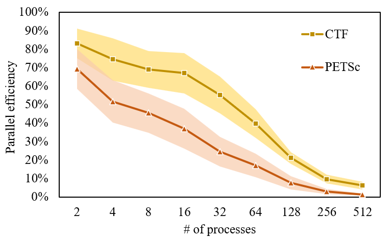

| SpGEMM | PETSc | CTF | |||||||||||||||||
| Processes | 2 | 4 | 8 | 16 | 32 | 64 | 128 | 256 | 512 | 1 | 2 | 4 | 8 | 16 | 32 | 64 | 128 | 256 | 512 |
| single | 1.39 | 2.07 | 3.64 | 5.91 | 7.83 | 10.91 | 9.81 | 7.52 | 7.02 | 0.29 | 0.40 | 0.65 | 1.27 | 2.37 | 4.65 | 7.37 | 7.11 | 4.90 | 5.36 |
| double | 1.40 | 2.15 | 3.59 | 5.74 | 7.98 | 10.69 | 11.06 | 7.79 | 6.72 | 0.34 | 0.52 | 0.91 | 1.59 | 3.14 | 6.00 | 10.41 | 10.88 | 7.50 | 7.72 |
7.5. Evaluation Results on Distributed System
The performance of CTF and PETSc on distributed system is evaluated in this section. Figure 20 summarizes their parallel efficiency, and their run time is compared in Table 11, which lists the average speedup to 1-process PETSc. It can be observed that CTF achieves higher parallel efficiency than PETSc in almost all processes settings, but its average performance is inferior to that of PETSc. For single precision, the average speedup of PETSc with all processes settings is higher than that of CTF. For double precision, however, the average speedup of CTF is close to that of PETSc at 64, 128, and 256 processes, and higher at 512 processes. Moreover, we find that CTF achieves a higher maximum speedup than PETSc for single-precision SpGEMM when the number of processes is larger than 32. For double-precision SpGEMM, it holds for all tested settings. In summary, PETSc achieves the better average performance than CTF, but CTF shows a better parallel efficiency and is expected to outperform PETSc when a large number of processes are available. Besides, we also compare the performance of CTF and PETSc with different floating-point precision. The experimental results from CTF show that the average speedup of single to double over all processes settings falls within the interval [1.04,1.11]. The interval becomes [1.21,1.40] for PETSc.
7.6. Evaluation Results of Preprocessing Overhead
Since other SpGEMM algorithms do not has a preprocessing stage, we only present the preprocessing overhead of MKL-CSR, MKL-BSR, and TileSpGEMM in this section. MKL-CSR includes two preprocessing operations: storing an input CSR matrix using the internal data structure (referred to as import), exporting the output matrix from the internal structure to the CSR (referred to as export). Although MKL-BSR is superior to MKL-CSR on a considerable number of matrices, it also requires extra preprocessing operation: format converting between CSR and BSR (referred to as convert). In TileSpGEMM, two input sparse matrices encoded with the CSR are required to be compressed using the tile structure (referred to as CSR2Tile), and the output matrix compressed with the tile structure is also required to be converted to the CSR (referred to as Tile2CSR).
Experimental results show that, for both MKL-CSR and MKL-BSR, the overhead of export is negligible, and import takes less than one SpGEMM on average. The convert in MKL-BSR is more time-consuming than other operations, taking about 8 SpGEMM on average. In TileSpGEMM, the format conversion between the tile structure and the CSR requires careful consideration, especially CSR2Tile, because it costs tens of single TileSpGEMM for some matrices. Tile2CSR has less time overhead than CSR2Tile, about 5 SpGEMM on average.
From the above discussion, we can conclude that most of the preprocessing overhead of SpGEMM comes from the format conversion. MKL-BSR, TileSpGEMM, and CUSP use BSR, tile structure, and COO format, respectively. All other SpGEMM algorithms use the popular CSR. Our evaluation on preprocessing overhead shows that the proposal of a new format requires careful consideration. It is necessary to evaluate the performance of SpGEMM in specific applications, simultaneously considering the overhead of format conversion.
8. Challenges and Future Work
SpGEMM has gained a lot of attention in recent decades, and the work has been conducted in many directions. We believe that it will be used in many other fields as the development of IoT, big data, and AI. We summarize some potential research directions and challenges as follows.
Optimization based on machine learning (ML). One of the challenges of SpGEMM is exploring the sparsity of sparse matrices. Researchers find that the non-zeros’ distribution dominates the performance of SpMV and SpGEMM on the same architecture. Over the past years, the parameter auto-tuning and automatic selection of sparse formats and SpMV algorithms based on ML models have been designed for SpMV optimization, and significant performance improvement has been observed. However, ML-based SpGEMM optimization is more challenging due to the sparsity consideration of three input sparse matrices, complicated matrix partitioning, and load balancing.
Optimization of size prediction. Among the four size prediction methods, upper-bound prediction may result in memory over-allocation, and progressive and probabilistic prediction may lead to memory re-allocation. Both over- and re-allocation are time-consuming for acceleration devices, such as GPU, DSP, FPGA, and TPU. On one hand, on-device memory capacity is limited and may not accommodate such a large amount of data. On the other head, it takes time to copy data to and from device memory because of separated memory space. Precise prediction is the most popular method. It not only reduces the overhead of memory management, but also indirectly improves the performance of result accumulating. However, we compared the run time of each stage in two-stage SpGEMM algorithms and found that the symbolic stage is even more expensive than the numerical stage for some matrices. Therefore, more efficient size prediction is required.
Heterogeneous architecture-oriented optimization. CPU is good at processing complicated logic, while the GPU is good at dense computations. Besides, DSP and FPGA may be used in different systems. One of the critical questions of porting SpGEMM to the heterogeneous system is how to achieve load balance and minimize communication traffic. Moreover, sub-matrices may have different non-zeros’ distribution. Ideally, relatively dense blocks should be mapped to acceleration devices, while ultra sparse blocks can be assigned to CPU. Only in this way can each device give full play to its architecture and optimize the overall computing performance of SpGEMM.
Application specific optimization. Application specific optimization of SpGEMM tends to be more useful and effective. Taking unsmoothed aggregation-based AMG for example, the sparse matrix of Galerkin product is a binary matrix with at most one non-zero entry per row. Therefore, the library AmgX (Naumov et al., 2015) develops a custom kernel to speed up the product. However, in classical AMG, is a tall-skinny sparse matrix. The calculating order of the Galerkin product, or , is important to the performance of hash accumulator-based SpGEMM. Specifically, tends to have less intermediate results accumulating overhead per row than (Naumov et al., 2015). Although the SpGEMM optimization based on application characteristics may reduce its extensibility, it is worthwhile if significant performance gains can be achieved. We expect more application characteristics to be fully exploited and utilized in the future.
SpMM is well-supported by existing hardware accelerators and GPU devices, as it is an important kernel of many convolutional algorithms. However, the sparsity of the matrices in convolution is much lower than that in HPC. Moreover, most high-performance computing units (such as tensor cores) only support the calculation of low floating-point precision (e.g. 16-bit half precision) because the precision is not so important in AI applications. This is not true for scientific and engineering computing, in which double precision is usually used for the convergence of solvers. Converting a sparse matrix to a dense one and running it on tensor cores are not promising as there are too much wasting work and extra overhead. SpGEMM is useful in the convolution algorithm if both the input and model are sparse. As the development of AI techniques, model pruning and optimization techniques, SpGEMM is expected to be supported in HPC devices.
9. Conclusion
The design of an efficient SpGEMM algorithm, as well as its implementation, is critical to many large-scale scientific applications. Therefore, it is not surprising that SpGEMM has attracted much attention from researchers over the years. In this survey, we highlight some developments in recent years and emphasize the applications, formulations, challenging problems, architecture-oriented optimizations, programming models, and performance evaluation. Some interesting conclusions can be summarized. Row-by-row is the most commonly used formulation because of its high parallelism and low cache requirement. CSR is the most frequently used storage format, as it is widely used in various fields and thus avoids expensive format conversion. SpGEMM in MKL presents the best performance on CPU. On GPU, spECK and NSparse outperform others and achieve the best performance on a large number of matrices. TileSpGEMM also shows excellent performance for regular and square matrices. On distributed system, PETSc is the winner when the number of processes is small. However, CTF presents better performance as the number of processes increases.
In conclusion, we stress the fact that despite recent progress, there are still important areas where much work remains to be done, such as different formats supporting, application and architecture-oriented optimization, and efficient size prediction. On the other hand, the heterogeneous architecture may give rise to new optimization opportunities, and efficient implementation in the specific architecture is within reach and can be expected to continue in the future.
Acknowledgements.
The authors would like to thank Zhaonian Tan and Yueyan Zhao for their early work. We would also like to extend our thanks to all reviewers for their constructive comments and suggestions. This work is supported by the Sponsor National Natural Science Foundation of China https://doi.org/10.13039/501100001809 under Grant No. Grant #61972033.References
- (1)
- Akbudak and Aykanat (2014) Kadir Akbudak and Cevdet Aykanat. 2014. Simultaneous Input and Output Matrix Partitioning for Outer-Product-Parallel Sparse Matrix-Matrix Multiplication. SIAM J. Sci. Comput. 36, 5 (2014), C568–C590. https://doi.org/10.1137/13092589X
- Akbudak and Aykanat (2017) Kadir Akbudak and Cevdet Aykanat. 2017. Exploiting Locality in Sparse Matrix-Matrix Multiplication on Many-Core Architectures. IEEE Trans. Parallel Distributed Syst. 28, 8 (2017), 2258–2271. https://doi.org/10.1109/TPDS.2017.2656893
- Akbudak et al. (2018) Kadir Akbudak, Oguz Selvitopi, and Cevdet Aykanat. 2018. Partitioning Models for Scaling Parallel Sparse Matrix-Matrix Multiplication. ACM Trans. Parallel Comput. 4, 3 (2018), 13:1–13:34. https://doi.org/10.1145/3155292
- Amossen et al. (2014) Rasmus Resen Amossen, Andrea Campagna, and Rasmus Pagh. 2014. Better Size Estimation for Sparse Matrix Products. Algorithmica 69, 3 (2014), 741–757. https://doi.org/10.1007/s00453-012-9692-9
- Anh et al. (2016) Pham Nguyen Quang Anh, Rui Fan, and Yonggang Wen. 2016. Balanced Hashing and Efficient GPU Sparse General Matrix-Matrix Multiplication. In Proceedings of the 2016 International Conference on Supercomputing, ICS 2016, Istanbul, Turkey, June 1-3, 2016, Ozcan Ozturk, Kemal Ebcioglu, Mahmut T. Kandemir, and Onur Mutlu (Eds.). ACM, 36:1–36:12. https://doi.org/10.1145/2925426.2926273
- ARB (2021) OpenMP ARB. 2021. OpenMP: The OpenMP API specification for parallel programming. https://www.openmp.org/
- Asanović et al. (2006) Krste Asanović, Ras Bodik, Bryan Christopher Catanzaro, Joseph James Gebis, Parry Husbands, Kurt Keutzer, David A. Patterson, William Lester Plishker, John Shalf, Samuel Webb Williams, and Katherine A. Yelick. 2006. The Landscape of Parallel Computing Research: A View from Berkeley. Technical Report UCB/EECS-2006-183. EECS Department, University of California, Berkeley. http://www2.eecs.berkeley.edu/Pubs/TechRpts/2006/EECS-2006-183.html
- Azad et al. (2016) Ariful Azad, Grey Ballard, Aydin Buluç, James Demmel, Laura Grigori, Oded Schwartz, Sivan Toledo, and Samuel Williams. 2016. Exploiting Multiple Levels of Parallelism in Sparse Matrix-Matrix Multiplication. SIAM J. Sci. Comput. 38, 6 (2016), C624–C651. https://doi.org/10.1137/15M104253X
- Azad et al. (2015) Ariful Azad, Aydin Buluç, and John R. Gilbert. 2015. Parallel Triangle Counting and Enumeration Using Matrix Algebra. In 2015 IEEE International Parallel and Distributed Processing Symposium Workshop, IPDPS 2015, Hyderabad, India, May 25-29, 2015. IEEE Computer Society, 804–811. https://doi.org/10.1109/IPDPSW.2015.75
- Azad et al. (2022) Ariful Azad, Oguz Selvitopi, Md Taufique Hussain, John R. Gilbert, and Aydin Buluç. 2022. Combinatorial BLAS 2.0: Scaling Combinatorial Algorithms on Distributed-Memory Systems. IEEE Trans. Parallel Distributed Syst. 33, 4 (2022), 989–1001. https://doi.org/10.1109/TPDS.2021.3094091
- Ballard et al. (2013) Grey Ballard, Aydin Buluç, James Demmel, Laura Grigori, Benjamin Lipshitz, Oded Schwartz, and Sivan Toledo. 2013. Communication optimal parallel multiplication of sparse random matrices. In 25th ACM Symposium on Parallelism in Algorithms and Architectures, SPAA ’13, Montreal, QC, Canada - July 23 - 25, 2013, Guy E. Blelloch and Berthold Vöcking (Eds.). ACM, 222–231. https://doi.org/10.1145/2486159.2486196
- Ballard et al. (2016a) Grey Ballard, Alex Druinsky, Nicholas Knight, and Oded Schwartz. 2016a. Hypergraph Partitioning for Sparse Matrix-Matrix Multiplication. ACM Trans. Parallel Comput. 3, 3 (2016), 18:1–18:34. https://doi.org/10.1145/3015144
- Ballard et al. (2016b) Grey Ballard, Christopher M. Siefert, and Jonathan J. Hu. 2016b. Reducing Communication Costs for Sparse Matrix Multiplication within Algebraic Multigrid. SIAM J. Sci. Comput. 38, 3 (2016), C203–C231. https://doi.org/10.1137/15M1028807
- Bell et al. (2012) Nathan Bell, Steven Dalton, and Luke N. Olson. 2012. Exposing Fine-Grained Parallelism in Algebraic Multigrid Methods. SIAM J. Scientific Computing 34, 4 (2012), C123–C152. https://doi.org/10.1137/110838844
- Borstnik et al. (2014) Urban Borstnik, Joost VandeVondele, Valéry Weber, and Jürg Hutter. 2014. Sparse matrix multiplication: The distributed block-compressed sparse row library. Parallel Comput. 40, 5-6 (2014), 47–58. https://doi.org/10.1016/j.parco.2014.03.012
- Briggs et al. (2000) William L. Briggs, Van Emden Henson, and Stephen F. McCormick. 2000. A multigrid tutorial, Second Edition. SIAM.
- Buluç and Gilbert (2008a) Aydin Buluç and John R. Gilbert. 2008a. Challenges and Advances in Parallel Sparse Matrix-Matrix Multiplication. In 2008 International Conference on Parallel Processing, ICPP 2008, September 8-12, 2008, Portland, Oregon, USA. IEEE Computer Society, 503–510. https://doi.org/10.1109/ICPP.2008.45
- Buluç and Gilbert (2008b) Aydin Buluç and John R. Gilbert. 2008b. On the representation and multiplication of hypersparse matrices. In 22nd IEEE International Symposium on Parallel and Distributed Processing, IPDPS 2008, Miami, Florida USA, April 14-18, 2008. IEEE, 1–11. https://doi.org/10.1109/IPDPS.2008.4536313
- Buluç and Gilbert (2010) Aydin Buluç and John R. Gilbert. 2010. Highly Parallel Sparse Matrix-Matrix Multiplication. CoRR abs/1006.2183 (2010). arXiv:1006.2183 http://arxiv.org/abs/1006.2183
- Buluç and Gilbert (2011) Aydin Buluç and John R. Gilbert. 2011. The Combinatorial BLAS: design, implementation, and applications. International Journal of High Performance Computing Applications 25, 4 (2011), 496–509. https://doi.org/10.1177/1094342011403516
- Buluç and Gilbert (2012) Aydin Buluç and John R. Gilbert. 2012. Parallel Sparse Matrix-Matrix Multiplication and Indexing: Implementation and Experiments. SIAM J. Sci. Comput. 34, 4 (2012), C170–C191. https://doi.org/10.1137/110848244
- Buluç and Madduri (2011) Aydin Buluç and Kamesh Madduri. 2011. Parallel breadth-first search on distributed memory systems. In Conference on High Performance Computing Networking, Storage and Analysis, SC 2011, Seattle, WA, USA, November 12-18, 2011, Scott A. Lathrop, Jim Costa, and William Kramer (Eds.). ACM, 65:1–65:12. https://doi.org/10.1145/2063384.2063471
- Cannon (1969) Lynn Elliot Cannon. 1969. A cellular computer to implement the Kalman filter algorithm. Montana State University.
- Çatalyürek et al. (2011) Ümit V. Çatalyürek, Bora Uçar, and Cevdet Aykanat. 2011. Hypergraph Partitioning. In Encyclopedia of Parallel Computing, David Padua (Ed.). Springer US, Boston, MA, 871–881. https://doi.org/10.1007/978-0-387-09766-4_1
- Censor-Hillel et al. (2015) Keren Censor-Hillel, Petteri Kaski, Janne H. Korhonen, Christoph Lenzen, Ami Paz, and Jukka Suomela. 2015. Algebraic Methods in the Congested Clique. In Proceedings of the 2015 ACM Symposium on Principles of Distributed Computing, PODC 2015, Donostia-San Sebastián, Spain, July 21 - 23, 2015, Chryssis Georgiou and Paul G. Spirakis (Eds.). ACM, 143–152. https://doi.org/10.1145/2767386.2767414
- Chan (2007) Timothy M. Chan. 2007. More Algorithms for All-pairs Shortest Paths in Weighted Graphs. In Proceedings of the Thirty-ninth Annual ACM Symposium on Theory of Computing (San Diego, California, USA) (STOC ’07). ACM, New York, NY, USA, 590–598. https://doi.org/10.1145/1250790.1250877
- Chen et al. (2017) Yu-Hsin Chen, Tushar Krishna, Joel S. Emer, and Vivienne Sze. 2017. Eyeriss: An Energy-Efficient Reconfigurable Accelerator for Deep Convolutional Neural Networks. IEEE J. Solid State Circuits 52, 1 (2017), 127–138. https://doi.org/10.1109/JSSC.2016.2616357
- Chen et al. (2019) Yuedan Chen, Kenli Li, Wangdong Yang, Guoqing Xiao, Xianghui Xie, and Tao Li. 2019. Performance-Aware Model for Sparse Matrix-Matrix Multiplication on the Sunway TaihuLight Supercomputer. IEEE Trans. Parallel Distributed Syst. 30, 4 (2019), 923–938. https://doi.org/10.1109/TPDS.2018.2871189
- Chen et al. (2020) Yuedan Chen, Guoqing Xiao, and Wangdong Yang. 2020. Optimizing partitioned CSR-based SpGEMM on the Sunway TaihuLight. Neural Comput. Appl. 32, 10 (2020), 5571–5582. https://doi.org/10.1007/s00521-019-04121-z
- Cohen (1997) Edith Cohen. 1997. Size-Estimation Framework with Applications to Transitive Closure and Reachability. J. Comput. Syst. Sci. 55, 3 (1997), 441–453. https://doi.org/10.1006/jcss.1997.1534
- Cohen (1998) Edith Cohen. 1998. Structure Prediction and Computation of Sparse Matrix Products. J. Comb. Optim. 2, 4 (1998), 307–332. https://doi.org/10.1023/A:1009716300509
- Cohen et al. (2009) Jeffrey Cohen, Brian Dolan, Mark Dunlap, Joseph M. Hellerstein, and Caleb Welton. 2009. MAD Skills: New Analysis Practices for Big Data. Proc. VLDB Endow. 2, 2 (2009), 1481–1492. https://doi.org/10.14778/1687553.1687576
- Cohen (2009) Jonathan D. Cohen. 2009. Graph Twiddling in a MapReduce World. Comput. Sci. Eng. 11, 4 (2009), 29–41. https://doi.org/10.1109/MCSE.2009.120
- Dalton et al. (2014) Steven Dalton, Nathan Bell, Luke Olson, and Michael Garland. 2014. Cusp: Generic Parallel Algorithms for Sparse Matrix and Graph Computations. http://cusplibrary.github.io/ , v0.5.0.
- Dalton et al. (2015) Steven Dalton, Luke N. Olson, and Nathan Bell. 2015. Optimizing Sparse Matrix - Matrix Multiplication for the GPU. ACM Trans. Math. Softw. 41, 4 (2015), 25:1–25:20. https://doi.org/10.1145/2699470
- Davis (2018) Timothy A. Davis. 2018. Graph algorithms via SuiteSparse: GraphBLAS: triangle counting and K-truss. In 2018 IEEE High Performance Extreme Computing Conference, HPEC 2018, Waltham, MA, USA, September 25-27, 2018. IEEE, 1–6. https://doi.org/10.1109/HPEC.2018.8547538
- Davis (2019) Timothy A. Davis. 2019. Algorithm 1000: SuiteSparse: GraphBLAS: Graph Algorithms in the Language of Sparse Linear Algebra. ACM Trans. Math. Softw. 45, 4 (2019), 44:1–44:25. https://doi.org/10.1145/3322125
- Davis and Hu (2011) Timothy A. Davis and Yifan Hu. 2011. The university of Florida sparse matrix collection. ACM Trans. Math. Softw. 38, 1 (2011), 1:1–1:25. https://doi.org/10.1145/2049662.2049663
- Demirci and Aykanat (2020a) Gunduz Vehbi Demirci and Cevdet Aykanat. 2020a. Cartesian Partitioning Models for 2D and 3D Parallel SpGEMM Algorithms. IEEE Trans. Parallel Distributed Syst. 31, 12 (2020), 2763–2775. https://doi.org/10.1109/TPDS.2020.3000708
- Demirci and Aykanat (2020b) Gunduz Vehbi Demirci and Cevdet Aykanat. 2020b. Scaling sparse matrix-matrix multiplication in the accumulo database. Distributed Parallel Databases 38, 1 (2020), 31–62. https://doi.org/10.1007/s10619-019-07257-y
- Demouth (2012) Julien Demouth. 2012. Sparse matrix-matrix multiplication on the GPU. In GPU Technology Conference 2012.
- Deveci et al. (2016) Mehmet Deveci, Erik G. Boman, Karen D. Devine, and Sivasankaran Rajamanickam. 2016. Parallel Graph Coloring for Manycore Architectures. In 2016 IEEE International Parallel and Distributed Processing Symposium, IPDPS 2016, Chicago, IL, USA, May 23-27, 2016. IEEE Computer Society, 892–901. https://doi.org/10.1109/IPDPS.2016.54
- Deveci et al. (2018a) Mehmet Deveci, Simon D. Hammond, Michael M. Wolf, and Sivasankaran Rajamanickam. 2018a. Sparse Matrix-Matrix Multiplication on Multilevel Memory Architectures : Algorithms and Experiments. CoRR abs/1804.00695 (2018). arXiv:1804.00695 http://arxiv.org/abs/1804.00695
- Deveci et al. (2013) Mehmet Deveci, Kamer Kaya, and Ümit V. Çatalyürek. 2013. Hypergraph Sparsification and Its Application to Partitioning. In 42nd International Conference on Parallel Processing, ICPP 2013, Lyon, France, October 1-4, 2013. IEEE Computer Society, 200–209. https://doi.org/10.1109/ICPP.2013.29
- Deveci et al. (2017) Mehmet Deveci, Christian Trott, and Sivasankaran Rajamanickam. 2017. Performance-Portable Sparse Matrix-Matrix Multiplication for Many-Core Architectures. In 2017 IEEE International Parallel and Distributed Processing Symposium Workshops, IPDPS Workshops 2017, Orlando / Buena Vista, FL, USA, May 29 - June 2, 2017. 693–702. https://doi.org/10.1109/IPDPSW.2017.8
- Deveci et al. (2018b) Mehmet Deveci, Christian Trott, and Sivasankaran Rajamanickam. 2018b. Multi-threaded Sparse Matrix-Matrix Multiplication for Many-Core and GPU Architectures. CoRR abs/1801.03065 (2018). arXiv:1801.03065 http://arxiv.org/abs/1801.03065
- Edwards et al. (2014) H. Carter Edwards, Christian R. Trott, and Daniel Sunderland. 2014. Kokkos: Enabling manycore performance portability through polymorphic memory access patterns. J. Parallel Distributed Comput. 74, 12 (2014), 3202–3216. https://doi.org/10.1016/j.jpdc.2014.07.003
- Elliott and Siefert (2018) James J Elliott and Christopher M Siefert. 2018. Low Thread-Count Gustavson: A Multithreaded Algorithm for Sparse Matrix-Matrix Multiplication Using Perfect Hashing. In 2018 IEEE/ACM 9th Workshop on Latest Advances in Scalable Algorithms for Large-Scale Systems (scalA). 57–64. https://doi.org/10.1109/ScalA.2018.00011
- Falgout (2006) Robert D. Falgout. 2006. An Introduction to Algebraic Multigrid. Comput. Sci. Eng. 8, 6 (2006), 24–33. https://doi.org/10.1109/MCSE.2006.105
- Filippone et al. (2017) Salvatore Filippone, Valeria Cardellini, Davide Barbieri, and Alessandro Fanfarillo. 2017. Sparse Matrix-Vector Multiplication on GPGPUs. ACM Trans. Math. Softw. 43, 4 (2017), 30:1–30:49. https://doi.org/10.1145/3017994
- Gadepally et al. (2015) Vijay Gadepally, Jake Bolewski, Dan Hook, Dylan Hutchison, Benjamin A. Miller, and Jeremy Kepner. 2015. Graphulo: Linear Algebra Graph Kernels for NoSQL Databases. CoRR abs/1508.07372 (2015). arXiv:1508.07372 http://arxiv.org/abs/1508.07372
- Gilbert et al. (1992) John R. Gilbert, Cleve Moler, and Robert Schreiber. 1992. Sparse Matrices in MATLAB: Design and Implementation. SIAM J. Matrix Anal. Appl. 13, 1 (1992), 333–356. https://doi.org/10.1137/0613024
- Gilbert et al. (2006) John R. Gilbert, Steven P. Reinhardt, and Viral B. Shah. 2006. High-Performance Graph Algorithms from Parallel Sparse Matrices. In Applied Parallel Computing. State of the Art in Scientific Computing, 8th International Workshop, PARA 2006, Umeå, Sweden, June 18-21, 2006, Revised Selected Papers (Lecture Notes in Computer Science, Vol. 4699), Bo Kågström, Erik Elmroth, Jack J. Dongarra, and Jerzy Wasniewski (Eds.). Springer, 260–269. https://doi.org/10.1007/978-3-540-75755-9_32
- Gilbert et al. (2008) John R. Gilbert, Steven P. Reinhardt, and Viral B. Shah. 2008. A Unified Framework for Numerical and Combinatorial Computing. Comput. Sci. Eng. 10, 2 (2008), 20–25. https://doi.org/10.1109/MCSE.2008.45
- Gondimalla et al. (2019) Ashish Gondimalla, Noah Chesnut, Mithuna Thottethodi, and T. N. Vijaykumar. 2019. SparTen: A Sparse Tensor Accelerator for Convolutional Neural Networks. In Proceedings of the 52nd Annual IEEE/ACM International Symposium on Microarchitecture, MICRO 2019, Columbus, OH, USA, October 12-16, 2019. ACM, 151–165. https://doi.org/10.1145/3352460.3358291
- Graphegon (2021) Graphegon. 2021. Pygraphblas. https://github.com/Graphegon/pygraphblas. Online; accessed 8 July 2022.
- Gremse et al. (2015) Felix Gremse, Andreas Höfter, Lars Ole Schwen, Fabian Kiessling, and Uwe Naumann. 2015. GPU-Accelerated Sparse Matrix-Matrix Multiplication by Iterative Row Merging. SIAM J. Sci. Comput. 37, 1 (2015). https://doi.org/10.1137/130948811
- Gu et al. (2020) Zhixiang Gu, Jose Moreira, David Edelsohn, and Ariful Azad. 2020. Bandwidth Optimized Parallel Algorithms for Sparse Matrix-Matrix Multiplication using Propagation Blocking. In SPAA ’20: 32nd ACM Symposium on Parallelism in Algorithms and Architectures, Virtual Event, USA, July 15-17, 2020, Christian Scheideler and Michael Spear (Eds.). ACM, 293–303. https://doi.org/10.1145/3350755.3400216
- Guidi et al. (2021a) Giulia Guidi, Marquita Ellis, Daniel Rokhsar, Katherine A. Yelick, and Aydin Buluç. 2021a. BELLA: Berkeley Efficient Long-Read to Long-Read Aligner and Overlapper. In Proceedings of the 2021 SIAM Conference on Applied and Computational Discrete Algorithms, ACDA 2021, Virtual Conference, July 19-21, 2021, Michael Bender, John Gilbert, Bruce Hendrickson, and Blair D. Sullivan (Eds.). SIAM, 123–134. https://doi.org/10.1137/1.9781611976830.12
- Guidi et al. (2021b) Giulia Guidi, Oguz Selvitopi, Marquita Ellis, Leonid Oliker, Katherine A. Yelick, and Aydin Buluç. 2021b. Parallel String Graph Construction and Transitive Reduction for De Novo Genome Assembly. In 35th IEEE International Parallel and Distributed Processing Symposium, IPDPS 2021, Portland, OR, USA, May 17-21, 2021. IEEE, 517–526. https://doi.org/10.1109/IPDPS49936.2021.00060
- Gustavson (1978) Fred G. Gustavson. 1978. Two Fast Algorithms for Sparse Matrices: Multiplication and Permuted Transposition. ACM Trans. Math. Softw. 4, 3 (1978), 250–269. https://doi.org/10.1145/355791.355796
- Haghi et al. (2020) Pouya Haghi, Tong Geng, Anqi Guo, Tianqi Wang, and Martin C. Herbordt. 2020. FP-AMG: FPGA-Based Acceleration Framework for Algebraic Multigrid Solvers. In 28th IEEE Annual International Symposium on Field-Programmable Custom Computing Machines, FCCM 2020, Fayetteville, AR, USA, May 3-6, 2020. IEEE, 148–156. https://doi.org/10.1109/FCCM48280.2020.00028
- Han et al. (2016) Song Han, Xingyu Liu, Huizi Mao, Jing Pu, Ardavan Pedram, Mark A. Horowitz, and William J. Dally. 2016. EIE: Efficient Inference Engine on Compressed Deep Neural Network. In 43rd ACM/IEEE Annual International Symposium on Computer Architecture, ISCA 2016, Seoul, South Korea, June 18-22, 2016. IEEE Computer Society, 243–254. https://doi.org/10.1109/ISCA.2016.30
- Hegde et al. (2019) Kartik Hegde, Hadi Asghari Moghaddam, Michael Pellauer, Neal Clayton Crago, Aamer Jaleel, Edgar Solomonik, Joel S. Emer, and Christopher W. Fletcher. 2019. ExTensor: An Accelerator for Sparse Tensor Algebra. In Proceedings of the 52nd Annual IEEE/ACM International Symposium on Microarchitecture, MICRO 2019, Columbus, OH, USA, October 12-16, 2019. ACM, 319–333. https://doi.org/10.1145/3352460.3358275
- Heroux et al. (2005) Michael A. Heroux, Roscoe A. Bartlett, Vicki E. Howle, Robert J. Hoekstra, Jonathan J. Hu, Tamara G. Kolda, Richard B. Lehoucq, Kevin R. Long, Roger P. Pawlowski, Eric T. Phipps, Andrew G. Salinger, Heidi Thornquist, Ray S. Tuminaro, James M. Willenbring, Alan B. Williams, and Kendall S. Stanley. 2005. An overview of the Trilinos project. ACM Trans. Math. Softw. 31, 3 (2005), 397–423. https://doi.org/10.1145/1089014.1089021
- Hussain et al. (2021) Md Taufique Hussain, Oguz Selvitopi, Aydin Buluç, and Ariful Azad. 2021. Communication-Avoiding and Memory-Constrained Sparse Matrix-Matrix Multiplication at Extreme Scale. In 35th IEEE International Parallel and Distributed Processing Symposium, IPDPS 2021, Portland, OR, USA, May 17-21, 2021. IEEE, 90–100. https://doi.org/10.1109/IPDPS49936.2021.00018
- Hutchison et al. (2015) Dylan Hutchison, Jeremy Kepner, Vijay Gadepally, and Adam Fuchs. 2015. Graphulo implementation of server-side sparse matrix multiply in the Accumulo database. In 2015 IEEE High Performance Extreme Computing Conference, HPEC 2015, Waltham, MA, USA, September 15-17, 2015. IEEE, 1–7. https://doi.org/10.1109/HPEC.2015.7322448
- Intel (2021) Intel. 2021. Intel Math Kernel Library. https://software.intel.com/en-us/mkl
- Ishiguro et al. (2020) Fumiya Ishiguro, Takahiro Katagiri, Satoshi Ohshima, and Toru Nagai. 2020. Performance Evaluation of Accurate Matrix-Matrix Multiplication on GPU Using Sparse Matrix Multiplications. In Eighth International Symposium on Computing and Networking Workshops, CANDAR 2020 Workshops, Naha, Japan, November 24-27, 2020. IEEE, 178–184. https://doi.org/10.1109/CANDARW51189.2020.00044
- Jamro et al. (2014) Ernest Jamro, Tomasz Pabis, Pawel Russek, and Kazimierz Wiatr. 2014. The Algorithms for FPGA Implementation of Sparse Matrices Multiplication. Comput. Informatics 33, 3 (2014), 667–684. http://www.cai.sk/ojs/index.php/cai/article/view/2795
- Jin and Ziavras (2004) Dejiang Jin and Sotirios G. Ziavras. 2004. A Super-Programming Technique for Large Sparse Matrix Multiplication on PC Clusters. IEICE Trans. Inf. Syst. 87-D, 7 (2004), 1774–1781. http://search.ieice.org/bin/summary.php?id=e87-d_7_1774
- Kanellopoulos et al. (2019) Konstantinos Kanellopoulos, Nandita Vijaykumar, Christina Giannoula, Roknoddin Azizi, Skanda Koppula, Nika Mansouri-Ghiasi, Taha Shahroodi, Juan Gómez-Luna, and Onur Mutlu. 2019. SMASH: Co-designing Software Compression and Hardware-Accelerated Indexing for Efficient Sparse Matrix Operations. In Proceedings of the 52nd Annual IEEE/ACM International Symposium on Microarchitecture, MICRO 2019, Columbus, OH, USA, October 12-16, 2019. ACM, 600–614. https://doi.org/10.1145/3352460.3358286
- Kaplan et al. (2006) Haim Kaplan, Micha Sharir, and Elad Verbin. 2006. Colored intersection searching via sparse rectangular matrix multiplication. In Proceedings of the 22nd ACM Symposium on Computational Geometry, Sedona, Arizona, USA, June 5-7, 2006, Nina Amenta and Otfried Cheong (Eds.). ACM, 52–60. https://doi.org/10.1145/1137856.1137866
- Kitchenham (2004) Barbara Ann Kitchenham. 2004. Procedures for Performing Systematic Reviews. Technical Report. Keele University, Department of Computer Science, Keele University, Kelee, UK. http://www.it.hiof.no/~haraldh/misc/2016-08-22-smat/Kitchenham-Systematic-Review-2004.pdf
- Kurt et al. (2017) Süreyya Emre Kurt, Vineeth Thumma, Changwan Hong, Aravind Sukumaran-Rajam, and P. Sadayappan. 2017. Characterization of Data Movement Requirements for Sparse Matrix Computations on GPUs. In 24th IEEE International Conference on High Performance Computing, HiPC 2017, Jaipur, India, December 18-21, 2017. IEEE Computer Society, 283–293. https://doi.org/10.1109/HiPC.2017.00040
- Lämmel (2008) Ralf Lämmel. 2008. Google’s MapReduce programming model - Revisited. Sci. Comput. Program. 70, 1 (2008), 1–30. https://doi.org/10.1016/j.scico.2007.07.001
- Lee et al. (2020) Jeongmyung Lee, Seokwon Kang, Yongseung Yu, Yong-Yeon Jo, Sang-Wook Kim, and Yongjun Park. 2020. Optimization of GPU-based Sparse Matrix Multiplication for Large Sparse Networks. In 36th IEEE International Conference on Data Engineering, ICDE 2020, Dallas, TX, USA, April 20-24, 2020. IEEE, 925–936. https://doi.org/10.1109/ICDE48307.2020.00085
- Li et al. (2019) Jiayu Li, Fugang Wang, Takuya Araki, and Judy Qiu. 2019. Generalized Sparse Matrix-Matrix Multiplication for Vector Engines and Graph Applications. In 2019 IEEE/ACM Workshop on Memory Centric High Performance Computing, MCHPC@SC 2019, Denver, CO, USA, November 18, 2019. IEEE, 33–42. https://doi.org/10.1109/MCHPC49590.2019.00012
- Lin et al. (2013) Colin Yu Lin, Ngai Wong, and Hayden Kwok-Hay So. 2013. Design space exploration for sparse matrix-matrix multiplication on FPGAs. Int. J. Circuit Theory Appl. 41, 2 (2013), 205–219. https://doi.org/10.1002/cta.796
- Liu et al. (2019) Junhong Liu, Xin He, Weifeng Liu, and Guangming Tan. 2019. Register-Aware Optimizations for Parallel Sparse Matrix-Matrix Multiplication. Int. J. Parallel Program. 47, 3 (2019), 403–417. https://doi.org/10.1007/s10766-018-0604-8
- Liu et al. (2021) Jiawen Liu, Jie Ren, Roberto Gioiosa, Dong Li, and Jiajia Li. 2021. Sparta: high-performance, element-wise sparse tensor contraction on heterogeneous memory. In PPoPP ’21: 26th ACM SIGPLAN Symposium on Principles and Practice of Parallel Programming, Virtual Event, Republic of Korea, February 27- March 3, 2021, Jaejin Lee and Erez Petrank (Eds.). ACM, 318–333. https://doi.org/10.1145/3437801.3441581
- Liu and Vinter (2014) Weifeng Liu and Brian Vinter. 2014. An Efficient GPU General Sparse Matrix-Matrix Multiplication for Irregular Data. In 2014 IEEE 28th International Parallel and Distributed Processing Symposium, Phoenix, AZ, USA, May 19-23, 2014. IEEE Computer Society, 370–381. https://doi.org/10.1109/IPDPS.2014.47
- Liu and Vinter (2015) Weifeng Liu and Brian Vinter. 2015. A framework for general sparse matrix-matrix multiplication on GPUs and heterogeneous processors. J. Parallel Distributed Comput. 85 (2015), 47–61. https://doi.org/10.1016/j.jpdc.2015.06.010
- Matam et al. (2012) Kiran Kumar Matam, Siva Rama Krishna Bharadwaj Indarapu, and Kishore Kothapalli. 2012. Sparse matrix-matrix multiplication on modern architectures. In 19th International Conference on High Performance Computing, HiPC 2012, Pune, India, December 18-22, 2012. IEEE Computer Society, 1–10. https://doi.org/10.1109/HiPC.2012.6507483
- Merrill and Grimshaw (2011) Duane Merrill and Andrew S. Grimshaw. 2011. High Performance and Scalable Radix Sorting: a Case Study of Implementing Dynamic Parallelism for GPU Computing. Parallel Process. Lett. 21, 2 (2011), 245–272. https://doi.org/10.1142/S0129626411000187
- Nagasaka et al. (2019) Yusuke Nagasaka, Satoshi Matsuoka, Ariful Azad, and Aydin Buluç. 2019. Performance optimization, modeling and analysis of sparse matrix-matrix products on multi-core and many-core processors. Parallel Comput. 90 (2019). https://doi.org/10.1016/j.parco.2019.102545
- Nagasaka et al. (2017) Yusuke Nagasaka, Akira Nukada, and Satoshi Matsuoka. 2017. High-Performance and Memory-Saving Sparse General Matrix-Matrix Multiplication for NVIDIA Pascal GPU. In 46th International Conference on Parallel Processing, ICPP 2017, Bristol, United Kingdom, August 14-17, 2017. IEEE Computer Society, 101–110. https://doi.org/10.1109/ICPP.2017.19
- Naumov et al. (2015) Maxim Naumov, M. Arsaev, Patrice Castonguay, Jonathan M. Cohen, Julien Demouth, Joe Eaton, Simon K. Layton, N. Markovskiy, István Z. Reguly, Nikolai Sakharnykh, V. Sellappan, and Robert Strzodka. 2015. AmgX: A Library for GPU Accelerated Algebraic Multigrid and Preconditioned Iterative Methods. SIAM J. Sci. Comput. 37, 5 (2015), S602–S626. https://doi.org/10.1137/140980260
- Niu et al. (2022) Yuyao Niu, Zhengyang Lu, Haonan Ji, Shuhui Song, Zhou Jin, and Weifeng Liu. 2022. TileSpGEMM: a tiled algorithm for parallel sparse general matrix-matrix multiplication on GPUs. In PPoPP ’22: 27th ACM SIGPLAN Symposium on Principles and Practice of Parallel Programming, Seoul, Republic of Korea, April 2 - 6, 2022, Jaejin Lee, Kunal Agrawal, and Michael F. Spear (Eds.). ACM, 90–106. https://doi.org/10.1145/3503221.3508431
- NVIDIA (2021) NVIDIA. 2021. Nvidia cuSPARSE library. https://developer.nvidia.com/cusparse
- Pal et al. (2018) Subhankar Pal, Jonathan Beaumont, Dong-Hyeon Park, Aporva Amarnath, Siying Feng, Chaitali Chakrabarti, Hun-Seok Kim, David T. Blaauw, Trevor N. Mudge, and Ronald G. Dreslinski. 2018. OuterSPACE: An Outer Product Based Sparse Matrix Multiplication Accelerator. In IEEE International Symposium on High Performance Computer Architecture, HPCA 2018, Vienna, Austria, February 24-28, 2018. IEEE Computer Society, 724–736. https://doi.org/10.1109/HPCA.2018.00067
- Parger et al. (2020) Mathias Parger, Martin Winter, Daniel Mlakar, and Markus Steinberger. 2020. spECK: accelerating GPU sparse matrix-matrix multiplication through lightweight analysis. In PPoPP ’20: 25th ACM SIGPLAN Symposium on Principles and Practice of Parallel Programming, San Diego, California, USA, February 22-26, 2020, Rajiv Gupta and Xipeng Shen (Eds.). ACM, 362–375. https://doi.org/10.1145/3332466.3374521
- Park et al. (2022) Sehun Park, Jae-Joon Kim, and Jaeha Kung. 2022. AutoRelax: HW-SW Co-Optimization for Efficient SpGEMM Operations With Automated Relaxation in Deep Learning. IEEE Trans. Emerg. Top. Comput. 10, 3 (2022), 1428–1442. https://doi.org/10.1109/TETC.2021.3089848
- Patwary et al. (2015) Md. Mostofa Ali Patwary, Nadathur Rajagopalan Satish, Narayanan Sundaram, Jongsoo Park, Michael J. Anderson, Satya Gautam Vadlamudi, Dipankar Das, Sergey G. Pudov, Vadim O. Pirogov, and Pradeep Dubey. 2015. Parallel Efficient Sparse Matrix-Matrix Multiplication on Multicore Platforms. In High Performance Computing - 30th International Conference, ISC High Performance 2015, Frankfurt, Germany, July 12-16, 2015, Proceedings (Lecture Notes in Computer Science, Vol. 9137), Julian M. Kunkel and Thomas Ludwig (Eds.). Springer, 48–57. https://doi.org/10.1007/978-3-319-20119-1_4
- Pentecost et al. (2019) Lillian Pentecost, Marco Donato, Brandon Reagen, Udit Gupta, Siming Ma, Gu-Yeon Wei, and David Brooks. 2019. MaxNVM: Maximizing DNN Storage Density and Inference Efficiency with Sparse Encoding and Error Mitigation. In Proceedings of the 52nd Annual IEEE/ACM International Symposium on Microarchitecture, MICRO 2019, Columbus, OH, USA, October 12-16, 2019. ACM, 769–781. https://doi.org/10.1145/3352460.3358258
- Pheatt (2008) Chuck Pheatt. 2008. Intel® threading building blocks. Journal of Computing Sciences in Colleges 23, 4 (2008), 298–298.
- Qin et al. (2021) Eric Qin, Geonhwa Jeong, William Won, Sheng-Chun Kao, Hyoukjun Kwon, Sudarshan Srinivasan, Dipankar Das, Gordon Euhyun Moon, Sivasankaran Rajamanickam, and Tushar Krishna. 2021. Extending Sparse Tensor Accelerators to Support Multiple Compression Formats. In 35th IEEE International Parallel and Distributed Processing Symposium, IPDPS 2021, Portland, OR, USA, May 17-21, 2021. IEEE, 1014–1024. https://doi.org/10.1109/IPDPS49936.2021.00110
- Qin et al. (2020) Eric Qin, Ananda Samajdar, Hyoukjun Kwon, Vineet Nadella, Sudarshan Srinivasan, Dipankar Das, Bharat Kaul, and Tushar Krishna. 2020. SIGMA: A Sparse and Irregular GEMM Accelerator with Flexible Interconnects for DNN Training. In IEEE International Symposium on High Performance Computer Architecture, HPCA 2020, San Diego, CA, USA, February 22-26, 2020. IEEE, 58–70. https://doi.org/10.1109/HPCA47549.2020.00015
- Rajamanickam et al. (2021) Sivasankaran Rajamanickam, Seher Acer, Luc Berger-Vergiat, Vinh Q. Dang, Nathan D. Ellingwood, Evan Harvey, Brian Kelley, Christian R. Trott, Jeremiah J. Wilke, and Ichitaro Yamazaki. 2021. Kokkos Kernels: Performance Portable Sparse/Dense Linear Algebra and Graph Kernels. CoRR abs/2103.11991 (2021). arXiv:2103.11991 https://arxiv.org/abs/2103.11991
- Ramanathan et al. (2021) Akshay Krishna Ramanathan, Srivatsa Srinivasa Rangachar, Hariram Thirucherai Govindarajan, Je-Min Hung, Chun-Ying Lee, Cheng-Xin Xue, Sheng-Po Huang, Fu-Kuo Hsueh, Chang-Hong Shen, Jia-Min Shieh, Wen-Kuan Yeh, Mon-Shu Ho, Jack Sampson, Meng-Fan Chang, and Vijaykrishnan Narayanan. 2021. CiM3D: Comparator-in-Memory Designs Using Monolithic 3-D Technology for Accelerating Data-Intensive Applications. IEEE Journal on Exploratory Solid-State Computational Devices and Circuits 7, 1 (2021), 79–87. https://doi.org/10.1109/JXCDC.2021.3087745
- Ramanathan et al. (2020) Akshay Krishna Ramanathan, Srivatsa Srinivasa Rangachar, Je-Min Hung, Chun-Ying Lee, Cheng-Xin Xue, Sheng-Po Huang, Fu-Kuo Hsueh, Chang-Hong Shen, Jia-Min Shieh, Wen-Kuan Yeh, Mon-Shu Ho, Hariram Thirucherai Govindarajan, Jack Sampson, Meng-Fan Chang, and Vijaykrishnan Narayanan. 2020. Monolithic 3D+-IC Based Massively Parallel Compute-in-Memory Macro for Accelerating Database and Machine Learning Primitives. In 2020 IEEE International Electron Devices Meeting (IEDM). 28.5.1–28.5.4. https://doi.org/10.1109/IEDM13553.2020.9372111
- Rasouli et al. (2021) Majid Rasouli, Robert M. Kirby, and Hari Sundar. 2021. A Compressed, Divide and Conquer Algorithm for Scalable Distributed Matrix-Matrix Multiplication. In HPC Asia 2021: The International Conference on High Performance Computing in Asia-Pacific Region, Virtual Event, Republic of Korea, January 20-21, 2021, Soonwook Hwang and Heon Young Yeom (Eds.). ACM, 110–119. https://doi.org/10.1145/3432261.3432271
- Rolinger et al. (2021) Thomas B. Rolinger, Christopher D. Krieger, and Alan Sussman. 2021. Optimizing Memory-Compute Colocation for Irregular Applications on a Migratory Thread Architecture. In 35th IEEE International Parallel and Distributed Processing Symposium, IPDPS 2021, Portland, OR, USA, May 17-21, 2021. IEEE, 58–67. https://doi.org/10.1109/IPDPS49936.2021.00015
- Rubensson and Rudberg (2014) Emanuel H. Rubensson and Elias Rudberg. 2014. Chunks and Tasks: A programming model for parallelization of dynamic algorithms. Parallel Comput. 40, 7 (2014), 328–343. https://doi.org/10.1016/j.parco.2013.09.006
- Rubensson and Rudberg (2016) Emanuel H. Rubensson and Elias Rudberg. 2016. Locality-aware parallel block-sparse matrix-matrix multiplication using the Chunks and Tasks programming model. Parallel Comput. 57 (2016), 87–106. https://doi.org/10.1016/j.parco.2016.06.005
- Sala et al. (2008) Marzio Sala, William F. Spotz, and Michael A. Heroux. 2008. PyTrilinos: High-performance distributed-memory solvers for Python. ACM Trans. Math. Softw. 34, 2 (2008), 7:1–7:33. https://doi.org/10.1145/1326548.1326549
- Selvitopi et al. (2019) Oguz Selvitopi, Gunduz Vehbi Demirci, Ata Turk, and Cevdet Aykanat. 2019. Locality-aware and load-balanced static task scheduling for MapReduce. Future Gener. Comput. Syst. 90 (2019), 49–61. https://doi.org/10.1016/j.future.2018.06.035
- Selvitopi et al. (2020a) Oguz Selvitopi, Saliya Ekanayake, Giulia Guidi, Georgios A. Pavlopoulos, Ariful Azad, and Aydin Buluç. 2020a. Distributed many-to-many protein sequence alignment using sparse matrices. In Proceedings of the International Conference for High Performance Computing, Networking, Storage and Analysis, SC 2020, Virtual Event / Atlanta, Georgia, USA, November 9-19, 2020, Christine Cuicchi, Irene Qualters, and William T. Kramer (Eds.). IEEE/ACM, 75. https://doi.org/10.1109/SC41405.2020.00079
- Selvitopi et al. (2020b) Oguz Selvitopi, Md Taufique Hussain, Ariful Azad, and Aydin Buluç. 2020b. Optimizing High Performance Markov Clustering for Pre-Exascale Architectures. In 2020 IEEE International Parallel and Distributed Processing Symposium (IPDPS), New Orleans, LA, USA, May 18-22, 2020. IEEE, 116–126. https://doi.org/10.1109/IPDPS47924.2020.00022
- Shivdikar (2021) Kaustubh Shivdikar. 2021. SMASH: Sparse Matrix Atomic Scratchpad Hashing. CoRR abs/2105.14156 (2021). arXiv:2105.14156 https://arxiv.org/abs/2105.14156
- Siegel et al. (2010) Jakob Siegel, Oreste Villa, Sriram Krishnamoorthy, Antonino Tumeo, and Xiaoming Li. 2010. Efficient sparse matrix-matrix multiplication on heterogeneous high performance systems. In 2010 IEEE International Conference On Cluster Computing Workshops and Posters (CLUSTER WORKSHOPS). 1–8. https://doi.org/10.1109/CLUSTERWKSP.2010.5613109
- Solomonik et al. (2014) Edgar Solomonik, Devin Matthews, Jeff R. Hammond, John F. Stanton, and James Demmel. 2014. A massively parallel tensor contraction framework for coupled-cluster computations. J. Parallel Distributed Comput. 74, 12 (2014), 3176–3190. https://doi.org/10.1016/j.jpdc.2014.06.002
- Soltaniyeh et al. (2020) Mohammadreza Soltaniyeh, Richard P. Martin, and Santosh Nagarakatte. 2020. Synergistic CPU-FPGA Acceleration of Sparse Linear Algebra. CoRR abs/2004.13907 (2020). arXiv:2004.13907 https://arxiv.org/abs/2004.13907
- Srikanth et al. (2020) Sriseshan Srikanth, Anirudh Jain, Joseph M. Lennon, Thomas M. Conte, Erik DeBenedictis, and Jeanine E. Cook. 2020. MetaStrider: Architectures for Scalable Memory-centric Reduction of Sparse Data Streams. ACM Trans. Archit. Code Optim. 16, 4 (2020), 35:1–35:26. https://doi.org/10.1145/3355396
- Srivastava et al. (2020) Nitish Kumar Srivastava, Hanchen Jin, Jie Liu, David H. Albonesi, and Zhiru Zhang. 2020. MatRaptor: A Sparse-Sparse Matrix Multiplication Accelerator Based on Row-Wise Product. In 53rd Annual IEEE/ACM International Symposium on Microarchitecture, MICRO 2020, Athens, Greece, October 17-21, 2020. IEEE, 766–780. https://doi.org/10.1109/MICRO50266.2020.00068
- Then et al. (2014) Manuel Then, Moritz Kaufmann, Fernando Chirigati, Tuan-Anh Hoang-Vu, Kien Pham, Alfons Kemper, Thomas Neumann, and Huy T. Vo. 2014. The More the Merrier: Efficient Multi-Source Graph Traversal. Proc. VLDB Endow. 8, 4 (2014), 449–460. https://doi.org/10.14778/2735496.2735507
- Trilinos Project Team (2020) The Trilinos Project Team. 2020. The Trilinos Home Page. https://trilinos.github.io. Online; (acccessed July 8, 2022).
- van de Geijn and Watts (1997) Robert A. van de Geijn and Jerrell Watts. 1997. SUMMA: scalable universal matrix multiplication algorithm. Concurr. Pract. Exp. 9, 4 (1997), 255–274. https://doi.org/10.1002/(SICI)1096-9128(199704)9:4<255::AID-CPE250>3.0.CO;2-2
- Vassilevska et al. (2006) Virginia Vassilevska, Ryan Williams, and Raphael Yuster. 2006. Finding heaviest H-subgraphs in real weighted graphs, with applications. CoRR abs/cs/0609009 (2006). arXiv:cs/0609009 http://arxiv.org/abs/cs/0609009
- Wang et al. (2019) Xiaoyun Wang, Zhongyi Lin, Carl Yang, and John D. Owens. 2019. Accelerating DNN Inference with GraphBLAS and the GPU. In 2019 IEEE High Performance Extreme Computing Conference, HPEC 2019, Waltham, MA, USA, September 24-26, 2019. IEEE, 1–6. https://doi.org/10.1109/HPEC.2019.8916498
- Weber et al. (2015) Valéry Weber, Teodoro Laino, Alexander Pozdneev, Irina Fedulova, and Alessandro Curioni. 2015. Semiempirical Molecular Dynamics (SEMD) I: Midpoint-Based Parallel Sparse Matrix-Matrix Multiplication Algorithm for Matrices with Decay. Journal of Chemical Theory and Computation 11, 7 (2015), 3145–3152. https://doi.org/10.1021/acs.jctc.5b00382 arXiv:https://doi.org/10.1021/acs.jctc.5b00382 PMID: 26575751.
- Winter et al. (2019) Martin Winter, Daniel Mlakar, Rhaleb Zayer, Hans-Peter Seidel, and Markus Steinberger. 2019. Adaptive sparse matrix-matrix multiplication on the GPU. In Proceedings of the 24th ACM SIGPLAN Symposium on Principles and Practice of Parallel Programming, PPoPP 2019, Washington, DC, USA, February 16-20, 2019, Jeffrey K. Hollingsworth and Idit Keidar (Eds.). ACM, 68–81. https://doi.org/10.1145/3293883.3295701
- Wolf et al. (2015) Michael M. Wolf, Jonathan W. Berry, and Dylan T. Stark. 2015. A task-based linear algebra Building Blocks approach for scalable graph analytics. In 2015 IEEE High Performance Extreme Computing Conference, HPEC 2015, Waltham, MA, USA, September 15-17, 2015. IEEE, 1–6. https://doi.org/10.1109/HPEC.2015.7322450
- Wolf et al. (2017) Michael M. Wolf, Mehmet Deveci, Jonathan W. Berry, Simon D. Hammond, and Sivasankaran Rajamanickam. 2017. Fast linear algebra-based triangle counting with KokkosKernels. In 2017 IEEE High Performance Extreme Computing Conference, HPEC 2017, Waltham, MA, USA, September 12-14, 2017. IEEE, 1–7. https://doi.org/10.1109/HPEC.2017.8091043
- Xia et al. (2021) Yang Xia, Peng Jiang, Gagan Agrawal, and Rajiv Ramnath. 2021. Scaling Sparse Matrix Multiplication on CPU-GPU Nodes. In 35th IEEE International Parallel and Distributed Processing Symposium, IPDPS 2021, Portland, OR, USA, May 17-21, 2021. IEEE, 392–401. https://doi.org/10.1109/IPDPS49936.2021.00047
- Xie and Liang (2019) Jiaming Xie and Yun Liang. 2019. SPART: Optimizing CNNs by Utilizing Both Sparsity of Weights and Feature Maps. In Advanced Parallel Processing Technologies - 13th International Symposium, APPT 2019, Tianjin, China, August 15-16, 2019, Proceedings (Lecture Notes in Computer Science, Vol. 11719), Pen-Chung Yew, Per Stenström, Junjie Wu, Xiaoli Gong, and Tao Li (Eds.). Springer, 71–85. https://doi.org/10.1007/978-3-030-29611-7_6
- Yasar et al. (2018) Abdurrahman Yasar, Sivasankaran Rajamanickam, Michael M. Wolf, Jonathan W. Berry, and Ümit V. Çatalyürek. 2018. Fast Triangle Counting Using Cilk. In 2018 IEEE High Performance Extreme Computing Conference, HPEC 2018, Waltham, MA, USA, September 25-27, 2018. IEEE, 1–7. https://doi.org/10.1109/HPEC.2018.8547563
- Yuster and Zwick (2005) Raphael Yuster and Uri Zwick. 2005. Fast sparse matrix multiplication. ACM Trans. Algorithms 1, 1 (2005), 2–13. https://doi.org/10.1145/1077464.1077466
- Zachariadis et al. (2020) Orestis Zachariadis, Nitin Satpute, Juan Gómez-Luna, and Joaquín Olivares. 2020. Accelerating sparse matrix-matrix multiplication with GPU Tensor Cores. Comput. Electr. Eng. 88 (2020), 106848. https://doi.org/10.1016/j.compeleceng.2020.106848
- Zhang et al. (2019) Feng Zhang, Weifeng Liu, Ningxuan Feng, Jidong Zhai, and Xiaoyong Du. 2019. Performance evaluation and analysis of sparse matrix and graph kernels on heterogeneous processors. CCF Trans. High Perform. Comput. 1, 2 (2019), 131–143. https://doi.org/10.1007/s42514-019-00008-6
- Zhang et al. (2021) Guowei Zhang, Nithya Attaluri, Joel S. Emer, and Daniel Sánchez. 2021. Gamma: leveraging Gustavson’s algorithm to accelerate sparse matrix multiplication. In ASPLOS ’21: 26th ACM International Conference on Architectural Support for Programming Languages and Operating Systems, Virtual Event, USA, April 19-23, 2021, Tim Sherwood, Emery D. Berger, and Christos Kozyrakis (Eds.). ACM, 687–701. https://doi.org/10.1145/3445814.3446702
- Zhang et al. (2011) Yudong Zhang, Lenan Wu, Geng Wei, and Shuihua Wang. 2011. A novel algorithm for all pairs shortest path problem based on matrix multiplication and pulse coupled neural network. Digit. Signal Process. 21, 4 (2011), 517–521. https://doi.org/10.1016/j.dsp.2011.02.004
- Zhang et al. (2020) Zhekai Zhang, Hanrui Wang, Song Han, and William J. Dally. 2020. SpArch: Efficient Architecture for Sparse Matrix Multiplication. In IEEE International Symposium on High Performance Computer Architecture, HPCA 2020, San Diego, CA, USA, February 22-26, 2020. IEEE, 261–274. https://doi.org/10.1109/HPCA47549.2020.00030