A Symbolic Regression Method for Dynamic Modeling
and Control
of Quadrotor UAVs
Abstract
This paper presents a mathematic dynamic model of a quadrotor unmanned aerial vehicle (QUAV) by using the symbolic regression approach and then proposes a hierarchical control scheme for trajectory tracking. The symbolic regression approach is capable of constructing analytical quadrotor dynamic equations only through the collected data, which relieves the burden of first principle modeling. To facilitate position tracking control of a QUAV, the design of controller can be decomposed into two parts: a proportional-integral controller for the position subsystem is first designed to obtain the desired horizontal position and the backstepping method for the attitude subsystem is developed to ensure that the Euler angles and the altitude can fast converge to the reference values. The effectiveness is verified through experiments on a benchmark multicopter simulator.
I Introduction
The study of unmanned aerial vehicles (UAVs) has attracted considerable attentions due to their wide applications in many areas including formation control, disaster assistance, monitoring patrol, environmental detection, and so on. The main advantages of a quadrotor lie in its simple mechanical structure, capability of taking off and landing vertically and favorable maneuverability. However, its dynamic characteristics, due to strong coupling, underactuated property and nonlinearity, make designing a controller for position tracking become complicated.
An accurate model is a significant factor that determines the performance of a controller. First principle modeling and data driven modeling are the two main approaches for dynamic modeling; see, e.g., [1, 2, 3, 4, 5, 6, 7]. The first principle modeling approach uses physical principles to derive a dynamic model. In particular, it analyzes the forces applied on the aircraft rotors and other modules, and derives the quadrotor dynamic equations utilizing mechanics and aerodynamics laws. For example, significant aerodynamic effects caused by the deformation of rotor blades were considered in [2]. The dynamic model constructed by this approach is capable of reflecting the flight behavior for more situations. However, the derivation process and the analytical form of the dynamic equations are usually complicated and hence the controller design becomes challenging.
The other modeling approach is to identify a dynamic model based on the collected input excitation and output response data from a real system. It is worth nothing that the accuracy of an identified model particularly depends on the identification algorithms and the collected data. Various identification techniques have been proposed in literature such as neural networks [4, 5], fuzzy-logic [6], reinforcement learning [7], and local linear regression [8], etc. However, these methods usually suffer from drawbacks including local linearization (local linear regression), complicated calculation and low interpretability (neural networks). In particular, the purely data driven methods can accurately fit system dynamics, however, they only offer a black box model rather than analytical dynamic equations. Therefore, many advanced control theories based on analytical models cannot be used.
In this paper, we adopt symbolic regression to construct a dynamic quadrotor model, which can somehow overcome the aforementioned disadvantages. In particular, this data driven approach gives an analytical model that captures the physical characteristics of the quadrotor dynamics and hence model based control theories can be applied.
Symbolic regression is an automated calculation approach that attempts to explore the inherent relationships only from data and establishes an interpretable model. A model constructed by symbolic regression does not require a pre-specified structure, which offers symbolic regression various potential applications [9, 10, 11, 12, 13, 14]. For instance, a meta-heuristic algorithm was developed in [9] to distill experimental data captured from various physical systems into analytical natural laws, including Hamiltonians, Lagrangians and other laws of geometric. Symbolic regression was adopted to find potential relation under the oil production data and made predictions for the peak of oil production in [10]. The work in [11] discovered an underlying multi-parameter model of a system and that in [12] revealed the important factors of the carbon emissions intensity using symbolic regression
In terms of tracking control for a quadrotor, researchers have presented various control techniques, such as dynamic inversion control [15], adaptive control [16, 17], backstepping control [18], sliding-mode control [19, 20], LMI-based linear control [21], and so on. These controllers have their features. To the best of our knowledge, few works have mentioned utilizing symbolic regression to construct an analytic model and a model-based control law. Therefore, we propose a tracking control scheme based on the analytic model obtained by symbolic regression.
From the above discussion, the main contribution of this paper is to use symbolic regression to build an accurate analytic QUAV model, based on which a hierarchical control scheme is designed for position tracking incorporating backstepping and dual-loop control techniques. Extensive experimental results on a benchmark multicopter simulator demonstrate the effectiveness of the proposed symbolic regression based model and the associated controller.
II Dynamic Modeling
In this section, we provide some background of a quadrotor dynamic model, discuss how symbolic regression is used for dynamic modeling, and then verify the effectiveness of the approach. The Matlab and PixHawk based multicopter simulator developed by the BUAA Reliable Flight Control Group [22] is used throughout the paper as the benchmark experiment platform.
II-A A Quadrotor UAV Model
A QUAV model represents a nonlinear system of four inputs and six degrees of freedom. It is composed of four individual electric motors and an X-shape airframe, as shown in Fig. 1. The torque and thrust can be changed by adjusting the rotation speed of each propeller, thereby further accomplishing different motions.
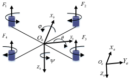
The dynamics of a quadrotor are explained using two reference frames. The inertial frame -- is defined relative to the ground, with the gravity pointing along the positive direction of the inertial axis. Let the vector denote the position of the center of mass in the inertial frame. The velocity and Euler angles of the quadrotor with respect to the inertial frame are represented by the vector and , respectively. The body frame -- is associated with the orientation of the quadrotor, with the thrust direction always consistent with the negative direction of the body axis. And the vector represents the angular velocity in the body frame. It is worthwhile pointing out that the roll and pitch angles are limited to () and the yaw angle is limited to (), which is physically meaningful. Then, the complete 12 dimensional state vector is denoted as
Let , , be the -th element of the vector . The control input represents the rotation speed of each motor, for . Denote . The dynamic model is of the following form
| (1) |
with the some functions , to be determined.
II-B Symbolic Regression Modeling
Symbolic regression (SR) is an established method that can effectively generate theories of causation in the form of mathematical equations from a collected data set. Unlike the traditional regression methods that require a fixed-form model derived from priori knowledge, SR automatically searches both the parameters and the form of equations. The expression of equations is composed of common functions (, , ), algebraic operators (, , , ), constants and relative variables. The selection of equations depends on its complexity and fitness. And the fitness function is widely used in SR, where denotes the input variable and the output variable, is the amount of pairs of input-output data , and is the equation learned by SR. Since the computation complexity caused by a large search space, genetic programming (GP) [23] is typically implemented in SR. GP is a meta-heuristic algorithm that adopts the principle of biological evolution to update candidate solutions.
In the initial phase of modeling, we generate multiple groups of random propeller rotation speeds within different ranges as the input data set. Then, by applying the input data set on the UAV simulator, we collect the output data set which includes velocity, acceleration, angular velocity, and angular acceleration. To perform symbolic regression modeling, we import the input and output data into the Eureqa software, select the formula building-blocks, e.g., and the absolute error metric for training. As a result, the analytic equations through efficient training and sifting are obtained as follows,
In particular, the functions , , represent the conversion relationship between and , which are considered as known transform equations. The remaining functions are obtained from different training data via symbolic regression. For instance, in order to acquire the function , we generate four groups of training data (2,000 samples) using the inputs in different ranges of 0-300rad/s, 0-700rad/s, 0-800rad/s and 0-1000rad/s. Both model validation and controller design are implemented on the equations learned from different training data, and the equation that performs the best is selected in the final model. The other functions in (1) are obtained in a similar way. It is worth mentioning that the propeller speeds for are constrained between 0 and 1000rad/s.
II-C Model Validation
To validate the learned dynamic model, a test data set is generated using the following excitation inputs for 10 seconds,
The reliability of the model is evaluated by comparing the six target variables ( obtained from the actual system and the SR model, respectively, and the result is shown in Fig. 2.
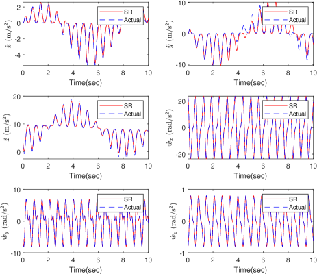
Generally speaking, symbolic regression can discover the accurate model equations beneath data, especially for angular acceleration , which indicates that symbolic regression is an effective modeling approach. Moreover, the RMSE, MAE and indexes are applied to quantitively reflect the approximation ability of SR; the results are summarized in Table I. The accuracy of the analytic model is negatively correlated with the values of RMSE, MAE and .
| Variable | RMSE | MAE | |
|---|---|---|---|
| 0.2632 | 0.2053 | 0.9707 | |
| 1.2655 | 0.8021 | 0.8781 | |
| 0.4011 | 0.2745 | 0.9907 | |
| 0.0034 | 0.0028 | 1.0000 | |
| 0.0013 | 0.0011 | 1.0000 | |
| 1.0000 |
III Control Design Scheme
In this section, we focus on the controller design for position and attitude tracking simutaneously. However, due to the underactuated property of a quadrotor, it is difficult to directly control the six state variables simultaneously. Therefore, the state variables to be controlled are chosen as and .
Let be the desired trajectories for , respectively. With
the control target is to achieve the following asymptotic tracking behaviors
| (2) |
and
| (3) |
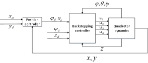
Given the reference position trajectory and the attitude angle , we can derive the reference attitude angles and hence the control laws for from a backstepping control scheme. To avoid complex calculation, we employ a hierarchical control strategy consisting of the outer-loop control for horizontal position as well as the inner-loop control for attitude and altitude. The block diagram of the overall control system is shown in Fig 3.
III-A Outer-loop controller design
The objective of this part is to design a proportional-integral (PI) controller for the outer loop subsystem to ensure the roll and pitch angles to be automatically tuned to drive the quadrotor to the desired horizontal position . Based on (1), the horizontal position subsystem is described as follows:
| (4) |
where and are regarded as the virtual controls to this subsystem.
More specifically, we aim to solve the desired angle trajectories for and , i.e., and , from the following equations
| (5) |
The solutions to (6) can be explicitly expressed as follows
| (6) |
When and achieve and , respectively, (to be elaborated in the next subsection), the closed-loop system (4) with and becomes
| (7) |
With proper selection of the parameters , , and , the control objective (2) can be achieved.
The design of and , as a virtual controller to the system (4), is of a PI structure containing the proportional terms and and the integral terms and , as well as feedforward compensation.
III-B Inner-loop controller design
In this part, a backstepping controller is designed to ensure and achieve and , respectively, for the objective (2) as explained in the previous subsection, that is,
| (8) |
for
Also, it is to ensure the objective (3). In other words, this subsection is concerned about the subsystem governing
| (10) | ||||
| (12) |
and the control objectives are (3) and (8) where are the desired trajectories and and designed in (6).
We introduce the following coordinate transformation
| (13) |
with
then the variables can be obtained as follows:
| (14) |
Now, the subsystem governing the states (12) can be equivalently transformed to a systems governing the following new state vector
| (16) |
Let be the -th element of , for . Now, the dynamics for can be reorganized as follows
| (17) |
where
and can be derived in a similar manner (with the details omitted). The vector represents the new control variables defined as follows
| (18) |
Let
Now, the objectives (3) and (8) are converted to design of for (17) such that
| (19) |
The design follows a backstepping procedure, see, e.g., [24]. First, we consider the Lyapunov function candidates
| (20) |
The derivative of along the trajectory of (17) satisfies
| (21) |
Here, is the virtual control whose desired value is
| (22) |
Let
| (23) |
Now, we consider the Lyapunov function candidates involving both and as follows
| (24) |
whose time derivative satisfies
Letting
| (25) |
gives
If the two parameters and are selected as positive constants, one has the target (19) achieved.
IV Numerical Experiments
In this section, the feasibility of symbolic regression modeling and the effectiveness of the proposed control scheme are validated on the benchmark quadrotor simulator developed in [22]. Ttwo cases of experiments are conducted. The main parameters of the QUAV are listed in Table II.
| Param | Value | Units | Definition |
|---|---|---|---|
| 1.4 | kg | Mass | |
| 9.8 | m/s2 | Gravity | |
| 0.0211 | kgm2 | Inertia moment | |
| 0.0219 | kgm2 | Inertia moment | |
| 0.0366 | kgm2 | Inertia moment | |
| 0.2250 | m | Fuselage radius | |
| N/(rad/s)2 | Thrust coefficient | ||
| Nm/(rad/s)2 | Moment coefficient |
Case I: The reference trajectories of the position and yaw angle are chosen as , , , and . With the initial condition: , , , The backstepping gains are specified as
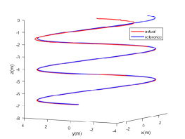
The position and yaw angle tracking trajectories are shown in Fig. 5, from which we can conclude that the QUAV can track the references with satisfactory performance. Moreover, the actual and desired position trajectories in 3-D space are shown in Fig. 5, which also demonstrate the accuracy of the model and the effectiveness of associated controller.
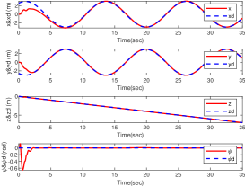
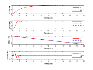
Case II: The control objective in this case is to achieve vertical take-off at a fixed horizontal position for the QUAV. The initial condition and the control gains are same as Case I. The reference trajectories are considered as , , , The experimental result is presented in Fig. 6. It is observed that the tracking errors asymptotically converge to a small range within 4 seconds, and the final steady-state errors are approximately zero.
V Conclusions
In this paper, we have proposed a novel modeling approach utilizing symbolic regression to construct the dynamic model of a QUAV. Based on the model constructed by symbolic regression, the PI and backstepping techniques were adopted to design a controller for time-varying position tracking. We have demonstrated the stability of the control system through theoretical analysis. Subsequently, simulation studies have shown that the proposed control scheme can achieve superior tracking performance, and symbolic regression is especially effective. Future work can focus on considering external disturbance, e.g., [25], and developing a robust control scheme based on symbolic regression.
References
- [1] N. S. Vanitha, L. Manivannan, T. Meenakshi, and K. Radhika, “Stability analysis of quadrotor using state space mathematical modeling,” Materials Today: Proceedings, 2020.
- [2] Y. R. Tang, X. Xiao, and Y. Li, “Nonlinear dynamic modeling and hybrid control design with dynamic compensator for a small-scale UAV quadrotor,” Measurement, p. S026322411730324X, 2017.
- [3] N. Abas, A. Legowo, Z. Ibrahim, N. Rahim, and A. M. Kassim, “Modeling and system identification using extended Kalman filter for a quadrotor system,” Applied Mechanics and Materials, vol. 313-314, pp. 976–981, 2013.
- [4] T. Dierks and S. Jagannathan, “Output feedback control of a quadrotor UAV using neural networks.,” IEEE Transactions on Neural Networks, vol. 21, no. 1, pp. 50–66, 2009.
- [5] S. Bansal, A. K. Akametalu, F. J. Jiang, F. Laine, and C. J. Tomlin, “Learning quadrotor dynamics using neural network for flight control,” in 2016 IEEE 55th Conference on Decision and Control (CDC), pp. 4653–4660, 2016.
- [6] S. A. Salman, V. R. Puttige, and S. G. Anavatti, “Real-time validation and comparison of fuzzy identification and state-space identification for a UAV platform,” in IEEE International Symposium on Computer Aided Control System Design, 2006.
- [7] J. L. Junell, T. Mannucci, Y. Zhou, and E. Van Kampen, “Self-tuning gains of a quadrotor using a simple model for policy gradient reinforcement learning,” in AIAA Guidance, Navigation, & Control Conference, 2016.
- [8] I. Grondman, M. Vaandrager, L. Busoniu, R. Babuska, and E. Schuitema, “Efficient model learning methods for actoc-critic control,” IEEE Transactions on Systems Man & Cybernetics Part B, vol. 42, no. 3, pp. 591–602, 2012.
- [9] M. Schmidt and H. Lipson, “Distilling free-form natural laws from experimental data,” Science, vol. 324, no. 5923, pp. 81–85, 2009.
- [10] G. Yang, X. Li, J. Wang, L. Lian, and T. Ma, “Modeling oil production based on symbolic regression,” Energy Policy, vol. 82, no. jul., pp. 48–61, 2015.
- [11] S. P. Chenna, G. Stitt, and H. Lam, “Multi-parameter performance modeling using symbolic regression,” in 2019 International Conference on High Performance Computing & Simulation (HPCS), 2019.
- [12] X. Pan, M. K. Uddin, B. Ai, X. Pan, and U. Saima, “Influential factors of carbon emissions intensity in oecd countries: Evidence from symbolic regression,” Journal of Cleaner Production, vol. 220, no. MAY 20, pp. 1194–1201, 2019.
- [13] E. Vladislavleva, T. Friedrich, F. Neumann, and M. Wagner, “Predicting the energy output of wind farms based on weather data: Important variables and their correlation,” Renewable Energy, vol. 50, no. FEB., pp. 236–243, 2013.
- [14] X. Wu, B. Xiao, and Y. Qu, “Modeling and sliding mode-based attitude tracking control of a quadrotor UAV with time-varying mass,” ISA Transactions, 2019.
- [15] A. Das, K. Subbarao, and F. Lewis, “Dynamic inversion with zero-dynamics stabilisation for quadrotor control,” Iet Control Theory & Applications, vol. 3, no. 3, pp. 303–314, 2009.
- [16] Z. Chen and J. Huang, “Attitude tracking and disturbance rejection of rigid spacecraft by adaptive control,” IEEE Transactions on Automatic Control, vol. 54, no. 3, pp. 600–605, 2009.
- [17] Z. Chen and J. Huang, “Attitude tracking of rigid spacecraft subject to disturbances of unknown frequencies,” International Journal of Robust & Nonlinear Control, vol. 24, no. 16, pp. 2231–2242, 2015.
- [18] F. Chen, R. Jiang, K. Zhang, B. Jiang, and G. Tao, “Robust backstepping sliding-mode control and observer-based fault estimation for a quadrotor UAV,” IEEE Transactions on Industrial Electronics, vol. 63, no. 8, pp. 5044–5056, 2016.
- [19] L. Luque-Vega, B. Castillo-Toledo, and A. G. Loukianov, “Robust block second order sliding mode control for a quadrotor,” Journal of the Franklin Institute, vol. 349, no. 2, pp. 719–739, 2012.
- [20] B. Zhao, B. Xian, Y. Zhang, and X. Zhang, “Nonlinear robust sliding mode control of a quadrotor unmanned aerial vehicle based on immersion and invariance method,” International Journal of Robust & Nonlinear Control, vol. 25, 2016.
- [21] T. Ryan and H. Jin Kim, “LMI-based gain synthesis for simple robust quadrotor control,” IEEE Transactions on Automation Science & Engineering, vol. 10, no. 4, pp. 1173–1178, 2013.
- [22] Q. Quan, Introduction to Multicopter Design and Control. Springer Singapore, 2017.
- [23] B.-T. Zhang and H. Mühlenbein, “Balancing accuracy and parsimony in genetic programming,” Evolutionary Computation, vol. 3, no. 1, pp. 17–38, 1995.
- [24] Z. Chen and J. Huang, “Global robust stabilization of cascaded polynomial systems,” Systems & control letters, vol. 47, no. 5, pp. 445–453, 2002.
- [25] Z. Chen, “A remark on sensor disturbance rejection of nonlinear systems,” IEEE Transactions on Automatic Control, vol. 54, no. 9, pp. 2206–2210, 2009.