A sub-pc BBH system in SDSS J1609+1756 through optical QPOs in ZTF light curves
Abstract
Optical quasi-periodic oscillations (QPOs) are the most preferred signs of sub-pc binary black hole (BBH) systems in AGN. In this manuscript, robust optical QPOs are reported in quasar SDSS J1609+1756 at . In order to detect reliable optical QPOs, four different methods are applied to analyze the 4.45 years-long ZTF g/r/i-band light curves of SDSS J1609+1756, direct fitting results by sine function, Generalized Lomb-Scargle periodogram, Auto-Cross Correlation Function and Weighted Wavelet Z-transform method. The Four different methods can lead to well determined reliable optical QPOs with periodicities days with confidence levels higher than 5, to guarantee the robustness of the optical QPOs in SDSS J1609+1756. Meanwhile, based on simulated light curves through CAR process to trace intrinsic AGN activities, confidence level higher than can be confirmed that the optical QPOs are not mis-detected in intrinsic AGN activities, re-confirming the robust optical QPOs and strongly indicating a central sub-pc BBH system in SDSS J1609+1756. Furthermore, based on apparent red-shifted shoulders in broad Balmer emission lines in SDSS J1609+1756, space separation of the expected central BBH system can be estimated to be smaller than light-days, accepted upper limit of total BH mass . Therefore, to detect and report BBH system expected optical QPOs with periodicities around 1 year is efficiently practicable through ZTF light curves, and combining with peculiar broad line emission features, further clues should be given on space separations of BBH systems in broad line AGN in the near future.
keywords:
galaxies:active - galaxies:nuclei - quasars:emission lines - quasars:individual (SDSS J1609+1756)1 Introduction
Binary black hole (BBH) systems on scale of sub-parsecs in central regions of active galactic nuclei (AGN), as well as dual core systems on scale of kpcs (or AGN pairs), are common as discussed in Begelman et al. (1980); Mayer et al. (2010); Fragione et al. (2019); Mannerkoski et al. (2022); Wang et al. (2023), considering galaxy merging as an essential process of galaxy formation and evolution (Kauffmann et al., 1993; Silk & Rees, 1998; Lin et al., 2004; Merritt, 2006; Bundy et al., 2009; Satyapal et al., 2014; Rodriguez-Gomez et al., 2017; Bottrell et al., 2019; Martin et al., 2021; Yoon et al., 2022). Meanwhile, in the manuscript, through discussions in more recent reviews in De Rosa et al. (2019); Chen et al. (2022), a kpc dual core system means central two BHs are getting closer due to dynamical frictions, but a sub-pc BBH system means central two BHs are getting closer mainly due to emission of gravitational waves. Besides indicators for BBH systems and/or dual core systems by spectroscopic features as discussed in Zhou et al. (2004); Komossa et al. (2008); Boroson & Lauer (2009); Smith et al. (2009); Shen & Loeb (2010); Eracleous et al. (2012); Comerford et al. (2013); Liu et al. (2016); Wang et al. (2017); De Rosa et al. (2019); Zhang (2021d) and by spatial resolved image properties as discussed in Komossa et al. (2003); Rodriguez et al. (2009); Piconcelli et al. (2010); Nardini (2017); Kollatschny et al. (2020), long-standing optical Quasi-Periodic Oscillations (QPOs) with periodicities around hundreds to thousands of days have been commonly accepted as the most preferred indicators for central BBH systems in AGN.
Long-standing optical QPOs have been reported in AGN related to central BBH systems in the literature. In the known quasar PG 1302-102, Graham et al. (2015a); Liu et al. (2018); Kovacevic et al. (2019) have shown detailed discussions on reliable 1800 days optical QPOs. Meanwhile, strong evidence have been reported to support optical QPOs in other individual AGN, such as 540 days QPOs in PSO J334.2028+01.4075 in Liu et al. (2015), 1500 days QPOs in SDSS J0159 in Zheng et al. (2016), 1150 days QPOs in Mrk915 in Serafinelli et al. (2020), 1.2 years QPOs in Mrk 231 in Kovacevic et al. (2020), 1607 days QPOs in SDSS J0252 in Liao et al. (2021), 6.4 years optical QPOs in SDSS J0752 in Zhang (2022a), 3.8 years optical QPOs in SDSS J1321 in Zhang (2022c), etc. Moreover, besides the optical QPOs reported in individual AGN, a sample of 111 candidates with optical QPOs have been reported in Graham et al. (2015) based on strong Keplerian periodic signals over a baseline of nine years, and a sample of 50 candidates with optical QPOs have been reported in Charisi et al. (2016).
While detecting BBH systems through optical QPOs, two important points have serious effects on reliability of BBH system expected QPOs. First, comparing with periodicities of detected optical QPOs, time durations of light curves are not longer enough to support reliabilities of the QPOs. Second, central AGN activities should lead to false optical QPOs, as well discussed in Vaughan et al. (2016); Sesana et al. (2018); Zhang (2022a, c). Thus, the reported confidence levels for reported optical QPOs through mathematical methods should be carefully re-checked. Currently, there are many public Sky Survey projects conveniently applied to search for long-standing optical QPOs. However, as the shown results in the largest sample of optical QPOs in Graham et al. (2015) and the other reported optical QPOs in individual AGN, the reported optical QPOs have periodicities commonly around 3.5 years (1500 days). Therefore, the Catalina Sky Survey (CSS, Drake et al. 2009) with longer time durations and moderate data quality of light curves is the preferred Sky Survey project for conveniently and systematically searching for optical QPOs with a few years long periodicities as the brilliant works in Graham et al. (2015). Meanwhile, comparing with the CSS project, the other Sky Survey projects have some disadvantages for searching for optical QPOs with ears-long periodicities, the Zwicky Transient Facility (ZTF, Bellm et al. 2019; Dekany et al. 2020) sky survey has light curves with short time durations (only around 4.5 years), the Panoramic Survey Telescope And Rapid Response System (PanSTARRS, Flewelling et al. 2020; Magnier et al. 2020) and the Sloan Digital Sky Survey Stripe82 (SDSS Stripe82, Bramich et al. 2008; Thanjavur et al. 2021) sky survey has light curves with large time steps, the All-Sky Automated Survey for Supernovae (ASAS-SN, Shappee et al. 2014; Kochanek et al. 2017) has light curves with limits for bright galaxies, etc. However, considering the high quality light curves in ZTF sky survey, optical QPOs with shorter periodicities (smaller than or around 1 year) should be preferred to be detected only through ZTF light curves, which is the main objective of the manuscript.
In this manuscript, a new BBH candidate is reported in SDSS J160911.25+175616.22 (=SDSS J1609+1756), a blue quasar at redshift 0.347, due to detected optical QPOs with periodicities about 340 days through more recent ZTF g/r/i-band light curves. Moreover, due to apparent red-shifted shoulders in broad Balmer emission lines, properties of peak separations of broad emission lines can be applied to determine limits of space separation of central BBH system in SDSS J1609+1756. The manuscript is organized as follows. Section 2 presents main results on the long-term optical variabilities of SDSS J1609+1756, and four different methods to detect robust optical QPOs in SDSS J1609+1756. Section 3 gives the main discussions including statistical results to support the optical QPOs not from central intrinsic AGN activities in SDSS J1609+1756, also including discussions on spectroscopic properties of SDSS J1609+1756, and discussions on basic structure information of space separation of central BBH system in SDSS J1609+1756. Section 4 gives final summary and main conclusions. In the manuscript, the cosmological parameters well discussed in Hinshaw et al. (2013) have been adopted as , and .

2 Optical QPOs in SDSS J1609+1756
2.1 Long-term optical light curves of SDSS J1609+1756
SDSS J1609+1756 is collected as target of the manuscript, due to two main reasons. First, as a candidate of off-nucleus AGN in Ward et al. (2021), SDSS J1609+1756 has peculiar broad Balmer lines with shifted red shoulders which can be well explained by broad line emissions from central two independent BLRs related to a central BBH system, quite similar as what we have recently discussed in Zhang (2021d). Second, after checking long-term variabilities of SDSS J1609+1756, apparent optical QPOs can be detected to support an expected BBH system.

The 4.45 years-long ZTF g/r/i-band light curves of SDSS J1609+1756 are collected and shown in top left panel of Fig 1, with MJD-58000 from 203 (Mar. 2018) to 1828 (Jul. 2022). Meanwhile, long-term light curves of SDSS J1609+1756 are also checked in CSS, PanSTARRS and ASAS-SN, and shown in Fig. 2 without apparent variabilities. There are 390 reliable data points included in the CSS light curve, however, as shown in left panel of Fig. 2, more than 92% of the 390 data points are lying between the range of mean magnitude plus/minus corresponding 1RMS scatters, indicating not apparent variabilities in the CSS light curve, probably due to lower quality of light curves. There are 1 reliable data point and 20 reliable data points included in the ASAS-SN V/g-band light curves shown in middle panel of Fig. 2. However, due to he quite large time steps with mean value about 200 days, it is not appropriate to search QPOs in ASAS-SN light curves. Similar as ASAS-SN g-band light curve, there are only 10 data points, 14 data points, 21 data points, 11 data points and 13 data points included in the PanSTARRS g/r/i/z/y-band light curves shown in right panel of Fig. 2, respectively, with large mean time steps about 266 days, 217 days, 184 days, 20 days and 182 days. Therefore, the PanSTARRS light curves are not considered in the manuscript.
Finally, the long-term ZTF light curves are mainly considered and there are no further discussions on variabilities from the other Sky Survey projects.

2.2 Methods to determine optical QPOs in SDSS J1609+1756
Based on the high-quality long-term optical light curves from ZTF, the following four methods are applied to detect optical QPOs in SDSS J1609+1756, similar as what have been done in Penil1 et al. (2020).
2.2.1 Direct fitting results by sine function
Based on a sine function plus a five-degree polynomial function applied to each ZTF light curve ( in units of days as time information, as )
| (1) |
, the ZTF g/r/i-band light curves can be well simultaneously described through the maximum likelihood method combining with MCMC (Markov Chain Monte Carlo) (Foreman-Mackey et al., 2013) technique with accepted well prior uniform distributions of the model parameters. Here, the only objective of applications of the model functions above is to check whether are there sine-like variability patterns (related to probable QPOs) included in the ZTF light curves, not to discuss physical origin of the sine-like variability patterns.
| g-band | 21.170.12 | -12.560.87 | 22.772.25 | -20.582.62 | 10.251.41 | -2.150.28 | 0.2330.006 | 2.5410.002 | 1.160.87 |
| r-band | 20.030.07 | -8.600.51 | 14.961.31 | -12.251.53 | 5.260.83 | -0.960.16 | 0.1500.005 | 2.5320.002 | 0.850.05 |
| i-band | 21.440.58 | -25.734.99 | 75.7515.81 | -107.2923.49 | 72.8316.42 | -18.794.33 | 0.1520.012 | 2.5530.004 | 1.900.21 |
Notice: The first column shows which band ZTF light curve is considered. The ninth column shows the determined model parameter periodicity with in units of days.
Then, based on the MCMC technique determined posterior distributions of the model parameters, the accepted model parameters and corresponding uncertainties are listed in Table 1. Here, we do not show posterior distributions of all the model parameters, but Fig 3 shows the MCMC technique determined two-dimensional posterior distributions of and periodicity of the ZTF g/r/i-band light curves. Meanwhile, based on the same functions, the Levenberg-Marquardt least-squares minimization technique (the known MPFIT package, Markwardt 2009) can lead to similar uncertainties of the model parameters, estimated through covariance matrix related to the determined model parameters, especially for . Therefore, the determined uncertainties of are reliable enough in SDSS J1609+1756. Moreover, in order to show more clearer sine variability patterns, the determined sine-like component is shown in dashed line in each ZTF light curve in top left panel of Fig. 1.
Based on the determined model parameters, left panels of Fig. 1 show the best fitting results and corresponding residuals (light curve minus the best fitting results) to each ZTF band light curve, leading (dof=885 as degree of freedom) to be 5.76. Meanwhile, after removing the five-degree polynomial component in each band light curve, accepted the determined periodicities , corresponding phase-folded light curves can also be well described by sine function with as phase information. The best fitting results and corresponding residuals to the folded ZTF g/r/i-band light curves are shown in right panels of Fig. 1, leading to .
Based on the results in Fig. 1, there are apparent optical QPOs with periodicities about days, days, days in the ZTF g/r/i-band light curves, respectively. The totally similar periodicities in the ZTF g/r/i-band light curves provide strong evidence to support the optical QPOs in SDSS J1609+1756. Moreover, considering shorter time duration of the ZTF i-band light curve, a bit difference between the periodicity in i-band light curve and the periodicities in g/r-band light curves can be accepted.

In order to confirm the apparent optical QPOs in ZTF light curves, rather than the model function shown in Equation (1), a N-degree (N=5, …, 30) polynomial function without any restrictions to model parameters is applied to re-describe each ZTF light curve. Fig. 4 shows dependence of re-determined by polynomial function on the degree of the polynomial function. It is clear that N26 can also lead to well accepted descriptions with to ZTF light curves of SDSS J1609+1756. Then, similar as what we have recently done in Zhang & Zhao (2022b), through determined different for model function (M1) in Equation (1) and for the 26-degree polynomial function (M2) applied, the calculated value is about
| (2) |
Based on and as number of dofs of the F distribution numerator and denominator, the expected confidence level is quite smaller than to support the 26-degree polynomial function. In other words, confidence level quite higher than 6 to support that the model function in Equation (1) is more preferred.
Therefore, based on the direct fitting results by sine function, there are apparent and reliable optical QPOs with periodicities about days, days, days in the ZTF g/r/i-band light curves, respectively. And, through the F-test technique, the sine component included in the ZTF light curves of SDSS J1609+1756 is more preferred with confidence level higher than 6.
2.2.2 Results from Generalized Lomb-Scargle (GLS) periodogram
In order to provide further evidence to support the optical QPOs in SDSS J1609+1756, besides the direct fitting results by sine function in Fig. 1, the widely accepted Generalized Lomb-Scargle (GLS) periodogram (Lomb, 1976; Scargle, 1982; Zechmeister & Kurster, 2009; VanderPlas, 2018) (included in the python package of astroML.time_series) is applied to check the periodicities in the observed ZTF g/r-band light curves in SDSS J1609+1756. Here, due to small number of data points and short time duration of the ZTF i-band light curve, the GLS periodogram is not applied to the i-band light curve. Top panel of Fig. 5 shows the GLS power properties. It is clear that there is one periodicity around 330 days with confidence level higher than (the false-alarm probability of 5e-7) determined by the bootstrap method as discussed in Ivezic et al. (2019).
Moreover, in order to determine uncertainties of GLS periodogram determined periodicity, the well-known bootstrap method is applied as follows. Through the observed ZTF g/r-band light curves, more than half of data points are randomly collected to re-build a new light curve. Then, within 20000 rebuild light curves after 20000 loops, the same GLS power properties are applied to determine new periodicities related to the rebuild light curves. Bottom panel of Fig. 5 shows distributions of corresponding 20000 GLS periodogram determined periodicities related to the 20000 rebuild light curves. And through the Gaussian-like distributions, the determined periodicities and corresponding uncertainties are 3192 days and 3445 days in the rebuild light curves through the g-band and r-band light curves, respectively, strongly reconfirming the smaller uncertainties of the periodicities determined by the MCMC technique. Moreover, through properties of g-band light curve, the tiny difference in the periodicity determined through different methods could be due to probably large uncertainties in g-band light curves leading the applied polynomial component to be not so appropriate. The GLS periodogram determined periodicities are consistent with results shown in Fig. 1, to confirm the optical QPOs in SDSS J1609+1756.


2.2.3 Results through the Auto-cross Correlation Function
Moreover, similar as what we have recently done on optical QPOs in Zhang (2022a, c), the Auto-cross Correlation Function (ACF) is applied to check optical QPOs in observed ZTF g/r-band light curves of SDSS J1609+1756. Corresponding results are shown in top panel of Fig. 6, totally similar periodicities around 340 days can be confirmed, to support the optical QPOs in SDSS J1609+1756. Here, direct linear interpolation is applied to the ZTF light curves, leading to evenly sampled light curves, and then the IDL procedure djs_correlate.pro (written by David Schlegel, Princeton) is applied to determine the correlation coefficients at different time lags.
Furthermore, the common Monte Carlo method is applied as follows to determine confidence level for ACF results. Accepted the time information of the observed ZTF g/r-band light curves of SDSS J1609+1756, 3.2 million light curves are randomly created by white noise process. For the th randomly created light curve of white noise, similar procedure is applied to determine the correlation coefficients, to determine the maximum coefficient (i=1, …, ) with time lags between 200 days and 500 days. Then, among all the 3.2 million values of , the maximum value of 0.4866 (0.46686) is determined as corresponding value for the 5 confidence level (probability of ) for the ACF results through the ZTF r-band (g-band) light curve. Therefore, the determined confidence level is higher than 5 for the ACF determined optical QPOs in SDSS J1609+1756.
Here, as well known that 5 corresponds to a probability of corresponding to about 1 in 3.2 million, therefore, 3.2 million light curves are created by white noise process, in order to determine 5 confidence level for ACF results (and also for the following WWZ results in the subsection 2.2.4). Furthermore, due to the following two main reasons, applications of red noise time series are not appropriate to determine 5 confidence levels of ACF results (and for the following WWZ results). On the one hand, ACF results for red noise time series can be described by an exponential function depending on intrinsic time intervals and correlation coefficients between adjacent data points. On the other hand, as more recent discussions in Krishnan et al. (2021), there are detections of fake periodic signals in red noise time series. Therefore, rather than red noise time series, white noise time series are preferred to be applied to determine confidence levels of ACF results (and the following WWZ results).
Meanwhile, similar bootstrap method is applied to determine uncertainties of ACF method determined periodicities in SDSS J1609+1756. Through the observed ZTF g/r-band light curves, more than half of data points are randomly collected to re-build a new light curve. Then, within 2000 rebuild light curves after 2000 loops, the ACF method is applied to determine new periodicities related to the rebuild light curves. Bottom panel of Fig. 6 shows distributions of corresponding 2000 ACF method determined periodicities related to the 2000 rebuild light curves. However, due to unevenly sampled ZTF light curves and applications linear interpolation, distributions in bottom panel of Fig. 6 are not well Gaussian-like, but standard deviations about 12 days and 10 days of the distributions can be safely accepted as uncertainties of ACF method determined periodicities through ZTF g-band and r-band light curves.
2.2.4 Results through the WWZ method
Moreover, similar as what we have recently done on optical QPOs in Zhang (2022a, c), the WWZ method (Foster, 1996; An et al., 2016; Gupta et al., 2018; Kushwaha et al., 2020; Li et al., 2021) is also applied to check the optical periodicities in the observed ZTF g/r-band light curves of SDSS J1609+1756. Corresponding results on both two dimensional power map properties and time-averaged power properties are shown in top and middle panels of Fig. 7, totally similar periodicities around 340 days can be confirmed, to support the optical QPOs in SDSS J1609+1756. Here, the python code wwz.py written by M. Emre Aydin is applied in the manuscript.
Meanwhile, the similar common Monte Carlo method is applied to determine confidence level for the WWZ determined results. Among the 3.2 million randomly created light curves for white noises, for the th randomly created light curve of white noise, maximum value of the WWZ method determined time-averaged power spectra can be well determined. Then, among all the 3.2 million values of , the maximum value of 26.64 (21.68) is determined as corresponding value for the 5 confidence level for the WWZ method determined time-averaged power properties through the ZTF g-band (r-band) light curve, which are shown in middle panel of Fig. 7. Therefore, the determined confidence level is higher than 5 for the WWZ method determined QPOs in SDSS J1609+1756.
Furthermore, the similar bootstrap method is applied to determine uncertainties of the WWZ method determined periodicities in SDSS J1609+1756. Through the observed ZTF g/r-band light curves, more than half of data points are randomly collected to re-build a new light curve. Then, within 800 rebuild light curves after 800 loops, the same WWZ method determined time-averaged power properties are applied to measure the new periodicities related to the rebuild light curves. Bottom panel of Fig. 7 shows distributions of corresponding WWZ method determined periodicities related to the 800 rebuild light curves. Through the Gaussian-like distributions, the determined periodicities and corresponding uncertainties are 3085 days and 35210 days in the rebuild light curves through the g-band and r-band light curves, respectively, to re-confirm the reliable optical QPOs in SDSS J1609+1756.
| Method | band | CL | |
|---|---|---|---|
| DF | g-band | 3482 | |
| r-band | 3402 | ||
| i-band | 3574 | ||
| GLS | g-band | 3192 | |
| r-band | 3445 | ||
| ACF | g-band | 32712 | |
| r-band | 30910 | ||
| WWZ | g-band | 3085 | |
| r-band | 35210 |
Notice: The first column shows which method is applied to determine optical QPOs in SDSS J1609+1756, DF means the ’direct fitting results to ZTF light curves’ as discussed in subsection 2.2.1. The second column shows which ZTF band light is considered. The third column shows the determined periodicity in units of days, the last column shows the determined corresponding confidence level.

2.2.5 Conclusion on the robustness of the optical QPOs in SDSS J1609+1756
Based on the different methods discussed above to detect reliable optical QPOs, Table 2 lists the necessary information of the periodicities and confidence levels. Therefore, the robust optical QPOs with periodicities around 340 days (0.93 years) in SDSS J1609+1756 can be detected and well confirmed from the 4.45 years-long ZTF light curves (time duration about 4.7 times longer than the detected periodicities) with confidence level higher than , based on the best-fitting results directly by the sine function shown in the left panels of Fig. 1, on the sine-like phase-folded light curve shown in the right panels of Fig. 1, on the results of GLS periodogram shown in Fig. 5, and on properties of ACF coefficients shown in Fig. 6 and on the power properties determined by the WWZ method shown in Fig. 7. The results cab be well applied to guarantee the robustness of the optical QPOs in SDSS J1609+1756.
Based on the well determined reliable and robust optical QPOs in SDSS J1609+1756, we can find that the periodicity around 340 days in SDSS J1609+1756 is so-far the smallest periodicity among the reported long-standing optical QPOs in normal broad line AGN in the literature as described in Introduction. The results are strongly indicating that BBH systems with shorter periodicities could be well detected through the ZTF sky survey project. More interestingly, to detect more optical QPOs related to BBH systems with shorter periodicities through ZTF light curves could provide more stronger BBH candidates for expected background gravitational wave signals at nano-Hz frequencies.


3 Main Discussions
3.1 Mis-detected optical QPOs related to central intrinsic AGN activities in SDSS J1609+1756?
Due to short time durations of ZTF light curves, it is necessary and interesting to check whether the determined optical QPOs was mis-detected QPOs tightly related to central intrinsic AGN activities of SDSS J1609+1756, although four different mathematical methods applied in the section above can provide robust evidence to support the detected optical QPOs in SDSS J1609+1756. Similar as what we have recently done in Zhang (2022a, c) to check probability of mis-detected QPOs in AGN activities in SDSS J0752 and in SDSS J1321, the following procedure is applied.
As well discussed in Kelly, Bechtold & Siemiginowska (2009); Kozlowski et al. (2010); MacLeod et al. (2010); Zu et al. (2013, 2016); Zhang & Feng (2017); Takata, Mukuta & Mizumoto (2018); Moreno et al. (2019); Sheng, Ross & Nicholl (2022), the known Continuous AutoRegressive (CAR) process and/or the improved Damped Random Walk (DRW) process can be applied to describe the fundamental AGN activities (Rees, 1984; Ulrich et al., 1997; Madejski & Sikora, 2016; Baldassare et al., 2020; Burke et al., 2021). Here, based on the DRW process, the public code JAVELIN (Just Another Vehicle for Estimating Lags In Nuclei) (Kozlowski et al., 2010; Zu et al., 2013) is firstly applied to describe the ZTF r-band light curve, with two process parameters of intrinsic characteristic variability amplitude and timescale of and . The best descriptions are shown in left panel of Fig. 8. And corresponding MCMC determined two dimensional posterior distributions of and are shown in right panel of Fig. 8, with the determined ( days) and . Here, because of the totally same periodicities through the ZTF r-band light curve by different methods in the section above, the r-band rather than the g-band light curve is considered in the section. Certainly, Fig. 8 also shows corresponding results through the g-band light curve.
Then, probability of mis-detected QPOs from DRW process described intrinsic AGN variabilities can be estimated as follows, through applications of the CAR process discussed in Kelly, Bechtold & Siemiginowska (2009):
| (3) |
with as a white noise process with zero mean and variance equal to 1. Here, the value 19.21, the mean value of the ZTF r-band light curve of SDSS J1609+1756, is set to be the mean value of . Then, a series of 100000 simulating light curves [, ] are created, with randomly selected from 100 days to 200 days (range of the determined of SDSS J1609+1756, after considering uncertainties). Then, variance of CAR process created light curve is set to be 0.168 which is the variance of ZTF r-band light curve of SDSS J1609+1756. And, time information are the same as the observational time information of ZTF r-band light curve of SDSS J1609+1756. And similar uncertainties are simply added to the simulating light curves , with and as the ZTF r-band light curve and corresponding uncertainties of SDSS J1609+1756.
Among the 100000 simulated light curves, there are 263 light curves collected with reliable mathematical determined periodicities according to the following four simple criteria. First, the simulated light curve can be well described by equation (1) with corresponding smaller than 8 ( in Fig. 1). Second, the simulated light curve has apparent GLS periodogram determined peak with corresponding periodicity smaller than 500 days with confidence level higher than . Third, the simulated light curve has apparent ACF and WWZ method determined peak with corresponding periodicity smaller than 500 days with confidence level higher than . Fourth, the determined periodicity by equation (1) is consistent with the GLS periodogram determined periodicity (which are similar as the ACF and WWZ method determined periodicities) within 10 times of the determined uncertainties by applications of equation (1). Left panel of Fig. 9 shows properties of the determined related to the best fitting results determined by equation (1) and the GLS periodogram determined periodicities (which are similar as the ACF and WWZ method determined periodicities) of the 263 simulated light curves. And right panel of Fig. 9 shows one of the 263 light curves with best fitting results by equation (1).
Therefore, even without any further considerations, it can be confirmed that the probability is only 0.26% (263/100000) (confidence level higher than ) to support mis-detected QPOs in CAR process simulated light curves related to AGN activities. Furthermore, accepted uncertainty days of optical periodicity in ZTF r-band light curve, if to limit periodicities within range from in the simulated light curves, there are only 112 simulated light curves collected, leading to the probability only about 0.11% (112/100000) (confidence level higher than ) to support mis-detected QPOs in AGN activities. In other words, the confidence level higher than to confirm the optical QPOs not from intrinsic AGN activities in SDSS J1609+1756, although short time durations in ZTF light curves, after well considering effects of AGN activities described by CAR process.


| line | flux | ||
|---|---|---|---|
| Broad H | 6556.512.19 | 54.201.43 | 1490.4963.93 |
| 6612.261.79 | 14.032.68 | 146.9937.27 | |
| Broad H | 4856.681.62 | 34.211.76 | 276.3117.27 |
| 4897.981.33 | 14.902.11 | 55.2212.05 | |
| He ii | 4686.630.64 | 3.200.64 | 14.362.60 |
| Narrow H | 6563.320.29 | 6.070.31 | 312.4516.95 |
| Narrow H | 4861.920.29 | 4.620.32 | 61.324.74 |
| [O iii]Å | 5007.720.03 | 3.570.05 | 580.0813.21 |
| 5005.390.59 | 8.650.69 | 99.3112.64 | |
| [O i]Å | 6300.880.88 | 5.200.84 | 34.905.07 |
| [O i]Å | 6365.121.56 | 8.851.67 | 38.026.48 |
| [N ii]Å | 6584.720.24 | 5.430.26 | 279.2116.53 |
| [S ii]Å | 6716.131.01 | 3.820.82 | 51.2316.54 |
| [S ii]Å | 6729.441.83 | 6.631.68 | 71.9317.82 |
Notice: The first column shows which line is measured. The Second, third, fourth columns show the measured Gaussian parameters: center wavelength in units of Å, line width (second moment) in units of Å and line flux in units of .
3.2 Spectroscopic properties of SDSS J1609+1756
Fig. 10 shows the SDSS spectrum with PLATE-MJD-FIBERID=2200-53875-0526 of SDSS J1609+1756 collected from SDSS DR16 (Ahumada et al., 2021). The apparent red-shifted shoulders, marked in Fig. 10, can be found in broad Balmer emission lines, as shown in Ward et al. (2021). And the shoulders should be more apparently determined after measurements of emission lines in SDSS J1609+1756 by the following emission line fitting procedure.
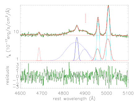
Multiple Gaussian functions can be applied to well simultaneously measure the emission lines around H within rest wavelength from 4600Å to 5100Å and around H within rest wavelength from 6150Å to 6850Å in SDSS J1609+1756, similar as what we have recently done in Zhang (2021a, b, c); Zhang & Zhao (2022b). Three broad and one narrow Gaussian functions are applied to describe broad and narrow components in H (H). And two narrow and two broad Gaussian functions are applied to describe [O iii]Å doublet, for the core components and for the components related to shifted wings. And one Gaussian function is applied to describe He iiÅ emission line. And six Gaussian functions are applied to describe the [O i]Å, [N ii]Å and [S ii]Å doublets. As the following shown best fitting results, it is not necessary to consider components related shifted wings in the [O i], [N ii] and [S ii] doublets. And, a power law function is applied to describe the AGN continuum emissions underneath the emission lines around H (H).
When the model functions are applied, only three restrictions are accepted. First, emission flux of each Gaussian emission component is not smaller than zero. Second, Gaussian components of each doublet have the same redshift. Third, corresponding Gaussian components in broad Balmer line have the same redshift. Then, through the Levenberg-Marquardt least-squares minimization technique (the known MPFIT package), best fitting results to emission lines can be determined and shown in Fig. 11 with . The measured parameters of each Gaussian component are listed in Table 3. Here, although three Gaussian functions are applied to describe each broad Balmer line, only two Gaussian components have reliable measured parameters which are at least 3times larger than their corresponding uncertainties, indicating two broad Gaussian components are enough to describe each broad Balmer line. Moreover, it is clear that there are red shifted shoulders in each broad Balmer emission line, especially based on the red-shifted broad Gaussian component in each broad Balmer line.
The main objective to discuss emission line properties of broad Balmer lines is that the shoulders can provide information on peak separation of two broad components coming from two BLRs related to an expected central BBH system, which will provide further clues on maximum space separation of the two black holes in the expected BBH system in SDSS J1609+1756. The red-shifted velocity of the shoulder in broad Balmer lines are about , based on the red-shift broad Gaussian component in each broad Balmer line. Meanwhile, peak separation in units of km/s related to a BBH system with space separation and with BH masses of and of the two BHs can be simply described as
| (4) |
with as inclination angle of the orbital plane to line-of-sight and as orientation angle of orbital phase. Therefore, considering the observed ( as blue-shifted velocity of undetected blue-shifted shoulders in broad Balmer lines in SDSS J1609+1756), the maximum space separation can be simply determined as
| (5) |
. Once there are clear information of central total BH mass which will be discussed in the next section, the maximum space separation can be well estimated.
3.3 Basic structure information of the expected BBH system in SDSS J1609+1756
For a broad line AGN, the virialization assumption accepted to broad line emission clouds is the most convenient method to estimate central virial BH mass as discussed in Peterson et al. (2004); Greene & Ho (2005); Vestergaard & Peterson (2006); Shen et al. (2011). However, considering mixed broad Balmer line emissions, it is difficult to determine the two clear components from central two independent BLRs related to central BBH system in SDSS J1609+1756, after checking the following point.
If the determined two broad Gaussian components in each broad Balmer line shown in Fig. 11 were truly related to a central BBH system, the virial BH mass as discussed in Greene & Ho (2005) of each BH in central region can be estimated as
| (6) |
with and ( and ) as line flux and line width (second moment) of red-shifted (blue-shifted) broad component in broad H, after considering the more recent empirical R-L relation to estimate BLRs sizes through line luminosity in Bentz et al. (2013). Then, under assumption of a BBH system, shift velocity ratio of red-shifted broad component to blue-shifted broad component in broad H can be estimated as
| (7) |
accepted the measured line widths and line fluxes and uncertainties listed in Table 3.
However, according to measured central wavelengths of the two broad components in broad H listed in Table 3, the observed shift velocity ratio is
| (8) |
with 6564.61 in units of Å as the theoretical value of central wavelength of broad H in rest frame, which is quite different from the . Therefore, although there are two broad Gaussian components determined in broad H, the two components are not appropriate to be applied to determine virial BH masses of central two black holes in the expected BBH system. Similar results can also be found through the two components in broad H.
Therefore, rather than virial BH mass estimated through broad line luminosity and broad line width, BH mass estimated by continuum luminosity as shown in Peterson et al. (2004) is determined as
| (9) |
with and in units of as continuum luminosity at 5100Å coming from central two BH accreting systems, then upper limit of central total BH mass can be estimated as
| (10) |
. Then, based on the fitting results shown in right panels of Fig. 11, total continuum luminosity at 5100Å in rest frame is . Simply accepted , upper limit of central total BH mass is about .
Accepted the estimated upper limit of total BH mass, the upper limit of space separation of the expected central BBH system in SDSS J1609+1756 is about
| (11) |
. Meanwhile, considering optical periodicity 340 days, as discussed in Eracleous et al. (2012), the space separation of the central BBH system can be estimated as
| (12) |
with accepted total BH mass . The space separation determined by periodicity is well below the upper limit of space separation determined by peak separation , not leading to clues against assumptions of the central BBH system in SDSS J1609+1756.
Before end of the subsection, one point should be noted. As simply discussed above, through optical periodicity 340 days, estimated space separation of the central BBH system is about 2.6 light-days in SDSS J1609+1756. Meanwhile, continuum luminosity about in SDSS J1609+1756 can lead BLRs sizes to be about 36 light-days through the R-L relation in Bentz et al. (2013), quite larger than light-days. Therefore, there should be few effects of dynamics of central BBH system on emission clouds of probably mixed BLRs in SDSS J1609+1756, or only apparent effects on emission clouds in inner regions of central mixed BLRs of SDSS J1609+1756. The results can provide further clues to support that it is not appropriate to estimate central BH mass by properties of broad emission lines in SDSS J1609+1756 as well discussed above, and also to support that the shifted velocity ratio discussed above should be not totally confirmed to be related to dynamics of central BBH system. Multi-epoch monitoring of variabilities of broad emission lines should provide further and accurate properties of dynamic structures of central expected BBH system in SDSS J1609+1756 in the near future.
3.4 Further discussions on the origin of optical QPOs in SDSS J1609+1756
Meanwhile, besides the expected central BBH system, precessions of emission regions with probable hot spots for the optical continuum emissions can also be applied to describe the detected optical QPOs in SDSS J1609+1756. As discussed in Eracleous et al. (1995) and in Storchi-Bergmann et al. (2003), the expected disk precession period can be estimated as
| (13) |
, with as distance of optical emission regions to central BH in units of 1000 Schwarzschild radii () and as the BH mass in units of . Considering optical periodicity about days and BH mass about above estimated through the continuum luminosity, the expected could be around 0.06 in SDSS J1609+1756.
However, based on the discussed distance of NUV emission regions to central BHs in Morgan et al. (2010) through the microlensing variability properties of eleven gravitationally lensed quasars, the NUV 2500Å continuum emission regions in SDSS J1609+1756 have distance from central BH as
| (14) |
leading size of NUV emission regions to be about . The estimated NUV emission regions have similar distances as the optical continuum emission regions in SDSS J1609+1756 under the disk precession assumption, strongly indicating that the disk precessions of emission regions are not preferred to be applied to explain the detected optical QPOs in SDSS J1609+1756.
Moreover, long-term QPOs can be detected in blazars due to jet precessions as discussed in Sandrinelli et al. (2018); Bhatta (2019); Otero-Santos et al. (2020). However, SDSS J1609+1756 is covered in Faint Images of the Radio Sky at Twenty-cm (Becker, White & Helfand, 1995; Helfand et al., 2015), but no apparent radio emissions. Therefore, jet precessions can be well ruled out to explain the optical QPOs in SDSS J1609+1756.
Furthermore, it is interesting to discuss whether the known relativistic Lense-Thirring precession (Cui, Zhang & Chen, 1998; Wagoner, 2012) can be applied to explain the detected optical QPOs in SDSS J1609+1756. As well discussed in Cui, Zhang & Chen (1998), observed periodicity related to the Lense-Thirring precession is about
| (15) |
with as redshift, as BH mass in units of , in units of as distance of emission regions in central accretion disk to central BH and (between 1) as dimensionless BH spin parameter. If accepted central BH mass as , minimum value of as (the estimated value for NUV emission regions above) for optical emission regions and maximum value , the minimum can be estimated to be about 5200days, about 13 times larger than the detected optical periodicity about 340days in SDSS J1609+1756. Therefore, the detected optical QPOs in SDSS J1609+1756 are not related to relativistic Lense-Thirring precessions.
Before ending of the manuscript, one point is noted. The SDSS J1609+1756 is collected from the candidates of off-nucleus AGN reported in the literature. However, it is not unclear whether are there tight connections between optical QPOs and off-nucleus AGN, studying on a sample of off-nucleus AGN with apparent optical QPOs could provide further clues on probable intrinsic connections in the near future.
4 Summary and Conclusions
The final summary and main conclusions are as follows.
-
•
The 4.45 years long-term ZTF g/r/i-band light curves can be well described by a sine function with periodicities about 340 days (about 0.9 years) with uncertainties about 4-5 days in SDSS J1609+1756, which can be further confirmed by the corresponding sine-like phase folded light curve with accepted periodicities, indicating apparent optical QPOs in SDSS J1609+1756.
-
•
Confidence level higher than can be confirmed to support the optical QPOs in SDSS J1609+1756 through applications of the Generalized Lomb-Scargle periodogram. Moreover, bootstrap method can be applied to re-determine small uncertainties about 5 days of the periodicities.
-
•
The reliable optical QPOs with periodicities 340 days with confidence level higher than 5 in SDSS J1609+1756 can also be confirmed by properties of ACF and WWZ methods, through the ZTF g/r-band light curves.
-
•
Robustness of the optical QPOs in SDSS J1609+1756 can be confirmed by the four different methods leading to totally similar periodicities with confidence level higher than 5.
-
•
Based on intrinsic AGN variabilities traced by the CAR process, confidence level higher than can be well determined to support the detect optical QPOs in SDSS J1609+1756 are not from intrinsic AGN activities, through a sample of 100000 CAR process simulated light curves. Therefore, the optical QPOs in SDSS J1609+1756 are more confident and robust, leading to an expected central BBH system in SDSS J1609+1756.
-
•
Although each broad Balmer emission line can be described by two Gaussian components, shifted velocity ratio determined through virial BH mass properties are totally different from the observed shifted velocity ratio through the measured central wavelengths of the two broad Gaussian components, indicating that applications of line parameters of the two broad Gaussian components are not preferred to estimate virial BH masses of central BHs, under the assumptions of an expected central BBH system in SDSS J1609+1756.
-
•
based on measured continuum luminosity at 5100Å in SDSS J1609+1756, central total BH mass can be estimated as . Then, based on the apparent shoulders in broad Balmer emission lines, upper limit of space separation of the expected central BBH system can be estimated as light-days in SDSS J1609+1756. And based on the optical periodicities, the space separation of the central BBH system can be estimated as light-days in SDSS J1609+1756, well below the estimated upper limit of space separation.
-
•
Based on the estimated size (distance to central BH) about of the NUV emission regions similar to the disk precession expected size about of the optical emission regions, the disk precessions can be not preferred to explain the detected optical QPOs in SDSS J1609+1756.
-
•
There are no apparent radio emissions in SDSS J1609+1756, strongly supporting that the jet precessions can be totally ruled out to explain the detected optical QPOs in SDSS J1609+1756.
Acknowledgements
Zhang gratefully acknowledge the anonymous referee for giving us constructive comments and suggestions to greatly improve our paper. Zhang gratefully acknowledges the kind grant support from NSFC-12173020 and NSFC-12373014. This paper has made use of the data from the SDSS projects, http://www.sdss3.org/, managed by the Astrophysical Research Consortium for the Participating Institutions of the SDSS-III Collaboration. This paper has made use of the data from the ZTF https://www.ztf.caltech.edu. The paper has made use of the public JAVELIN code (http://www.astronomy.ohio-state.edu/~yingzu/codes.html#javelin), and the MPFIT package https://pages.physics.wisc.edu/~craigm/idl/cmpfit.html, and the emcee package https://emcee.readthedocs.io/en/stable/, and the wwz.py code http://github.com/eaydin written by M. Emre Aydin. This research has made use of the NASA/IPAC Extragalactic Database (NED, http://ned.ipac.caltech.edu) which is operated by the California Institute of Technology, under contract with the National Aeronautics and Space Administration.
Data Availability
The data underlying this article will be shared on reasonable request to the corresponding author ([email protected]).
References
- Ahumada et al. (2021) Ahumada, R.; Prieto, C. A.; Almeida, A.; et al., 2021, ApJS, 249, 3
- An et al. (2016) An, T.; Lu, X.; Wang, J., 2016, A&A, 585, 89
- Baldassare et al. (2020) Baldassare, V. F.; Geha, M.; Greene, J., 2020, ApJ, 896, 10
- Becker, White & Helfand (1995) Becker, R. H., White, R. L., Helfand, D. J. 1995, ApJ, 450, 559
- Begelman et al. (1980) Begelman, M. C., Blandford, R. D., Rees, M. J., 1980, Natur, 287, 307
- Bellm et al. (2019) Bellm E. C., Kulkarni, S. R.; Barlow, T., et al., 2019, PASP, 131, 068003
- Bentz et al. (2013) Bentz M. C., Denney, K. D.; Grier, C. J.; et al., 2013, ApJ, 767, 149
- Bhatta (2019) Bhatta, G., 2019, Universe Proceedings, 17, 15, arXiv:1909.10268
- Boroson & Lauer (2009) Boroson, T. A., Lauer, T. R. 2009, Nature, 458, 53
- Bottrell et al. (2019) Bottrell, C.; Hani, M. H.; Teimoorinia, H.; et al., 2019, MNRAS, 490, 5390
- Bramich et al. (2008) Bramich, D. M.; Vidrih, S.; Wyrzykowski, L.; et al., 2008, MNRAS, 386, 887
- Bundy et al. (2009) Bundy, K.; Fukugita, M.; Ellis, R. S.; Targett, T. A.; Belli, S.; Kodama, T., 2009, ApJ, 697, 1369
- Burke et al. (2021) Burke, C. J.; Shen, Y.; Blaes, O., et al., 2021, Sci, 373, 789
- Charisi et al. (2016) Charisi, M.; Bartos, I.; Haiman, Z.; et al., 2016, MNRAS, 463, 2145
- Chen et al. (2022) Chen, Y. C.; Hwang, H. C.; Shen, Y.; Liu, X.; Zakamska, N. L.. Yang, Q.; Li, J. I., 2022, ApJ, 925, 162
- Comerford et al. (2013) Comerford, J. M., Schluns, K., Greene, J. E., Cool, R. J., 2013, ApJ, 777, 64
- Cui, Zhang & Chen (1998) Cui, W.; Zhang, S. N.; Chen, W., 1998, ApJL, 492, L53
- Dekany et al. (2020) Dekany, R.; Smith, R. M.; Riddle, R., et al., 2020, PASP, 132, 038001
- De Rosa et al. (2019) De Rosa, A.; Vignali, C.; Bogdanovic, T., et al., 2019, NewAR, 86, 101525
- Drake et al. (2009) Drake, A. J.; Djorgovski, S. G.; Mahabal, A., et al., 2009, ApJ, 696, 870
- Eracleous et al. (1995) Eracleous, M.; Livio M.; Halpern, J. P., 1995, ApJ, 438, 610
- Eracleous et al. (2012) Eracleous, M.; Boroson, T. A.; Halpern, J. P.; Liu, J., 2012, ApJS, 201, 23
- Flewelling et al. (2020) Flewelling, H. A.; Magnier, E. A.; Chambers, K. C.; et al., 2020, ApJS, 251, 7
- Foreman-Mackey et al. (2013) Foreman-Mackey, D.; Hogg, D. W.; Lang, D.; Goodman, J., 2016, PASP, 125, 306
- Foster (1996) Foster, G., 1996, AJ, 112, 1709
- Fragione et al. (2019) Fragione, G.; Grishin, E.; Leigh, N. W. C.; Perets, H. B.; Perna, R., 2019, MNRAS, 488, 47
- Graham et al. (2015a) Graham, M. J.; Djorgovski, S. G.; Stern, D., et al., 2015a, Natur, 518, 74
- Graham et al. (2015) Graham, M. J., Djorgovski, S. G., Stern, D., et al., 2015, MNRAS, 453, 1562
- Greene & Ho (2005) Green, J. E., Ho, L. C., 2005, ApJ, 630, 122
- Gupta et al. (2018) Gupta, A. C.; Tripathi, A.; Wiita, P. J.; et al., 2018, A&A, 616, 6
- Helfand et al. (2015) Helfand, D. J.; White, R. L.; Becker, R. H., 2015, ApJ, 801, 26
- Hinshaw et al. (2013) Hinshaw, G.; Larson, D.; Komatsu, E.; et al., 2013, ApJS, 208, 19
- Ivezic et al. (2019) Ivezic, Z.; Connolly, A. J.; VanderPlas, J. T.; Gray, A. 2019, Statistics, Data Mining, and Machine Learning in Astronomy: A Practical Python Guide for the Analysis of Survey Data, ISBN: 9780691197050, Princeton University Press
- Kauffmann et al. (1993) Kauffmann, G.; White, S. D. M.; Guiderdoni, B., 1993, MNRAS, 264, 201
- Kelly, Bechtold & Siemiginowska (2009) Kelly, B. C.; Bechtold, J.; Siemiginowska, A., 2009, ApJ, 698, 895
- Kochanek et al. (2017) Kochanek, C. S.; Shappee, B. J.; Stanek, K. Z.; et al., 2017, PASP, 129, 4502
- Kollatschny et al. (2020) Kollatschny, W.; Weilbacher, P. M.; Ochmann, M. W.; Chelouche, D.; Monreal-Ibero, A.; Bacon, R.; Contini, T., 2020, A&A, 633, 79
- Komossa et al. (2003) Komossa, S., Burwitz, V., Hasinger, G., Predehl, P., Kaastra, J. S., Ikebe, Y., 2003, ApJL, 582, L15
- Komossa et al. (2008) Komossa, S., Zhou, H., Lu, H. 2008, ApJ, 678, L81
- Kovacevic et al. (2019) Kovacevic, A. B., Popovic, L. C., Simic, S., Ilic, D., 2019, ApJ, 871, 32
- Kovacevic et al. (2020) Kovacevic, A. B.; Yi, T.; Dai, X.; et al., 2020, MNRAS, 494, 4069
- Kozlowski et al. (2010) Kozlowski, S.; Kochanek, C. S.; Udalski, A., et al., 2010, ApJ, 708, 927
- Krishnan et al. (2021) Krishnan, S.; Markowitz, A. G.; Schwarzenberg-Czerny, A.; Middleton, M. J., 2021, MNRAS, 508, 3975
- Kushwaha et al. (2020) Kushwaha, P.; Sarkar, A.; Gupta, Alok C.; Tripathi, A.; Wiita, P. J., 2020, MNRAS, 499, 653
- Li et al. (2021) Li, X.; Cai, Y.; Yang, H.; Luo, Y.; Yan, Y.; He, J.; Wang, L., 2021, MNRAS, 506, 2540
- Liao et al. (2021) Liao, W.; Chen, Y.; Liu, X.; et al., 2021, MNRAS, 500, 4025
- Lin et al. (2004) Lin, L.; Koo, D. C.; Willmer, C. N. A.; et al., 2004, ApJL, 617, 9
- Liu et al. (2016) Liu, J., Eracleous, M., Halpern, J. P., 2016, ApJ, 817, 42
- Liu et al. (2015) Liu, T., Gezari, S., Heinis, S., et al., 2015, ApJL, 803, L16
- Liu et al. (2018) Liu, T., Gezari, S., Miller M. C., 2018, ApJL, 859, L12
- Lomb (1976) Lomb, N. R. 1976, Ap&SS, 39, 447
- MacLeod et al. (2010) MacLeod, C. L., Ivezic, Z., Kochanek, C. S., et al., 2010, ApJ, 721, 1014
- Madejski & Sikora (2016) Madejski, G.; Sikora, M., 2016, ARA&A, 54, 725
- Magnier et al. (2020) Magnier, E. A.; Chambers, K. C.; Flewelling, H. A.; et al., 2020, ApJS, 251, 3
- Mannerkoski et al. (2022) Mannerkoski, M.; Johansson, P. H.; Rantala, A.; Naab, T.; Liao, S.; Rawlings, A., 2022, ApJ, 929, 167
- Markwardt (2009) Markwardt, C. B., 2009, Astronomical Data Analysis Software and Systems XVIII ASP Conference Series, Vol. 411, proceedings of the conference held 2-5 November 2008 at Hotel Loews Le Concorde, Quebec City, QC, Canada. Edited by David A. Bohlender, Daniel Durand, and Patrick Dowler. San Francisco: Astronomical Society of the Pacific, p.251
- Martin et al. (2021) Martin, G.; Jackson, R. A.; Kaviraj, S., et al., 2021, MNRAS, 500, 4937
- Mayer et al. (2010) Mayer, L., Kazantzidis, S., Escala, A., Callegari, S., 2010, Natur, 466, 1082
- Merritt (2006) Merritt, D., 2006, ApJ, 648, 976
- Morgan et al. (2010) Morgan, C. W.; Kochanek, C. S.; Morgan, N. D.; Falco, E. E., 2010, ApJ, 712, 1129
- Moreno et al. (2019) Moreno, J.; Vogeley, M. S.; Richards, G. T.; Yu, W., 2019, PASP, 131, 3001
- Nardini (2017) Nardini, E., 2017, MNRAS, 471, 3483
- Otero-Santos et al. (2020) Otero-Santos, J.; Acosta-Pulido, J. A.; Becerra Gonzalez, J.; et al., 2020, MNRAS, 492, 5524
- Penil1 et al. (2020) Penil1, P.; Dominguez1, A.; Buson, S.; et al., 2020, ApJ, 896, 134
- Peterson et al. (2004) Peterson B. M.; Ferrarese, L.; Gilbert, K. M., et al., 2004, ApJ, 613, 682
- Piconcelli et al. (2010) Piconcelli, E., Vignali, C., Bianchi, S., et al., 2010, ApJL 722, L147
- Rees (1984) Rees, M. J., 1984, ARA&A, 22, 471
- Rodriguez et al. (2009) Rodriguez, C., Taylor, G. B., Zavala, R. T., Pihlstrom, Y. M., Peck, A. B., 2009, ApJ, 697, 37
- Rodriguez-Gomez et al. (2017) Rodriguez-Gomez, V.; Sales, L. V.; Genel, S., et al., 2017, MNRAS, 467, 3083
- Sandrinelli et al. (2018) Sandrinelli, A.; Covino, S.; Treves, A.; et al., 2018, A&A, 615, 118
- Satyapal et al. (2014) Satyapal, S.; Ellison, S. L.; McAlpine, W.; Hickox, R. C.; Patton, D. R.; Mendel, J. T., 2014, MNRAS, 441, 1297
- Scargle (1982) Scargle, J. D. 1982, ApJ, 263, 835
- Sesana et al. (2018) Sesana, A.; Haiman, Z.; Kocsis, B.; Kelley, L. Z., 2018, ApJ, 856, 42
- Serafinelli et al. (2020) Serafinelli, R.; Severgnini, P.; Braito, V., et al., 2020, ApJ, 902, 10
- Shappee et al. (2014) Shappee, B. J.; Prieto, J. L.; Grupe, D.; et al., 2014, ApJ, 788, 48
- Shen & Loeb (2010) Shen, Y.; Loeb, A., 2010, ApJ, 725, 249
- Shen et al. (2011) Shen, Y.; Richards, G. T.; Strauss, M. A; et al., 2011, ApJS, 194, 4
- Sheng, Ross & Nicholl (2022) Sheng, X.; Ross, N.; Nicholl, M., 2022, MNRAS, 512, 5580
- Silk & Rees (1998) Silk, J.; Rees, M. J. 1998, A&A, 331, L1
- Smith et al. (2009) Smith, K. L., Shields, G. A., Bonning, E. W., McMullen, C. C., Salviander, S. 2009, ApJ, 716, 866
- Storchi-Bergmann et al. (2003) Storchi-Bergmann, T.; Nemmen da Silva, R., Eracleous, M., et al., 2003, ApJ, 598, 956
- Takata, Mukuta & Mizumoto (2018) Takata, T.; Mukuta, Y.; Mizumoto, Y., 2018, ApJ, 869, 178
- Thanjavur et al. (2021) Thanjavur, K.; Ivezic, Z.; Allam, S. S.; Tucker, D. L.; Smith, J. A.; Gwyn, S., 2021, MNRAS, 505, 5941
- Ulrich et al. (1997) Ulrich, M. H.; Maraschi, L.; Urry, C. M., 1997, ARA&A, 35, 445
- VanderPlas (2018) VanderPlas, J. T., 2018, ApJS, 236, 16
- Vaughan et al. (2016) Vaughan, S.; Uttley, P.; Markowitz, A. G.; et al., 2016, MNRAS, 461, 3145
- Vestergaard & Peterson (2006) Vestergaard, M., Peterson, B. M. 2006, ApJ, 641, 689
- Ward et al. (2021) Ward, C.; Gezari, S.; Frederick, S., et al., 2021, ApJ, 913, 102
- Wang et al. (2017) Wang, L., Greene, J. E., Ju, W., Rafikov, R. R., Ruan J. J., Schneider, D. P., 2017, ApJ, 834, 129
- Wang et al. (2023) Wang, J.; Songsheng, Y.; Li, Y.; Du, P., 2023, MNRAS, 518, 3397
- Wagoner (2012) Wagoner, R. V., 2012, ApJL, 752, L18
- Yoon et al. (2022) Yoon, Y.; Park, C.; Chung, H.; Lane, R. R., 2022, ApJ, 925, 168
- Zechmeister & Kurster (2009) Zechmeister, M.; Kurster, M., 2009, A&A, 496, 577
- Zhang & Feng (2017) Zhang, X. G., Feng L. L., 2017, MNRAS, 464, 2203
- Zhang (2021a) Zhang, X. G., 2021a, MNRAS, 502, 2508
- Zhang (2021b) Zhang, X. G., 2021b, ApJ, 909, 16, arXiv2101.02465
- Zhang (2021c) Zhang, X. G., 2021c, ApJ accepted, arXiv2107.09214
- Zhang (2021d) Zhang, X. G., 2021d, MNRAS, 507, 5205, arXiv:2108.09714
- Zhang (2022a) Zhang, X. G., 2022a, MNRAS, 512, 1003, arXiv:2202.11995
- Zhang & Zhao (2022b) Zhang, X. G., Zhao S., 2022b, ApJ, 937, 105, ArXiv:2209.02164
- Zhang (2022c) Zhang, X. G., 2022c, MNRAS, 516, 3650, arXiv:2209.01923
- Zheng et al. (2016) Zheng, Z.; Butler, N. R.; Shen, Y.; et al., 2016, ApJ, 827, 56
- Zhou et al. (2004) Zhou, H., Wang, T., Zhang, X., Dong, X., Li, C. 2004, ApJL, 604, L33
- Zu et al. (2013) Zu, Y.; Kochanek, C. S.; Kozlowski, S.; Udalski, A., 2013, ApJ, 765, 106
- Zu et al. (2016) Zu, Y.; Kochanek, C. S.; Kozlowski, S.; Peterson, B. M., 2016, ApJ, 819, 122