A Study of Quantitative Correlations Between Crucial Bio-markers and the Optimal Drug Regimen of Type-I Lepra Reaction

CH Ramanjaneyulu First Author. Email: [email protected] Dinesh Nayak Second author. Email: [email protected] D K K Vamsi Centre for Excellence in Mathematical Biology, Sri Sathya Sai Institute of Higher Learning, India. Corresponding author. Email: [email protected]

Abstract

Leprosy (Hansen’s) is a disease caused by Mycobacterium leprae. This disease slowly leads to occurrence of leprae reactions which mainly damage peripheral nervous system which cause loss of organs. We can prevent occurring leprae reactions by monitoring the bio-markers involved in it. Motivated by these observations in this research work we do a exhaustive study dealing with the quantitative correlations between crucial bio-markers and the Multi Drug Thearphy (MDT) used in treating the type I lepra reaction. We frame and study a complex 11 compartment model dealing with the the concentrations of plasma $c_{1}(t)$ and effective drug action $c_{2}(t)$ , susceptible schwann cells $S(t)$ , infected schwann cells $I(t)$ , bacterial load $B(t)$ , and five cytokines pivotal in Type-1 Lepra reaction: IFN- $\gamma$ , TNF- $\alpha$ , IL- $10$ , IL- $12$ , IL- $15$ , and IL- $17$ . We explore exhaustively and establish the quantitative correlations with respect to the optimal drug dosage of the MDT drugs such as rifampin, clofazimine & dapsone and the crucial bio-markers involved in type I lepra reaction. We conclude this work by reitrating the fact that the optimal drug dosage of the MDT drugs found through these optimal control studies and the dosage prescribed as per WHO guidelines are almost the same.

keywords: Hansen’s disease, Type I lepra reaction, bio-markers, multidrug therapy, Newton’s gradient method, optimal drug regimen

MSC 2020 codes: 37Nxx, 92BXX, 92Cxx

1 Introduction

Leprosy, one of the oldest diseases has remained a neglected tropical disease long since. It is caused primarily by slow-growing bacterium Mycobacterium leprae (M. leprae). This bacterium primarily affects Schwann cells, leading to skin damage and impacting the peripheral nervous system, as well as affecting the eyes and mucosa of the upper respiratory tract. According to the World Health Organization (WHO), over 200,000 new cases of leprosy are reported annually in approximately 120 countries [1]. In 2022, India alone recorded about 103,819 new cases [2]. Leprosy is transmitted via droplets from the nose and mouth during close and frequent contact with untreated cases. Leprosy can progress to a chronic phase known as Lepra reaction, resulting in permanent disabilities and organ loss. Early detection of the disease through monitoring key changes in biomarker levels is crucial for preventing these consequences.

The modeling of leprosy began in the 1970s with simple compartmental models, such as the susceptible-infectious-recovered framework [3]. Subsequently, more complex models were developed to assess the effectiveness of long-term control and elimination strategies, including mass drug administration, contact tracing, and vaccination [4]. Several investigations focusing on the population-level dynamics of the disease are discussed in studies [5, 6]. Additionally, the work [7] deal with the cellular dynamics within the host.

The alterations in the chemical and metabolic properties of the cytosolic environment within host cells due to the presence of M. leprae were first elucidated by Rudolf Virchow (1821–1902) in the late nineteenth century [8]. Subsequent clinical studies have delineated the pathways of cytokine responses, leading to the identification of two main types of Lepra reactions. Type-1 Lepra reactions are associated with cellular immune responses, while Type-2 reactions are linked to humoral immune responses [9, 10]. Both pathways involve crucial biomarkers/cytokines such as $IFN-\gamma$ , $TNF-\alpha$ , $IL-10$ , $IL-12$ , $IL-15$ , and $IL-17$ [11]. Numerous biochemical studies have investigated the pathogenesis of lepra reaction [12], as well as the growth of the bacteria and its chemical consequences [11].

Motivated by these observations, the authors have done a comprehensive studies dealing with the qualitative correlations between crucial bio-markers and the Multi Drug Thearphy (MDT) used in treating the type I lepra reaction. More details of the same can be found in the references [13, 14].

In the present work we explore and do a exhaustive study of quantitative correlations between crucial bio-markers and the Multi Drug Thearphy (MDT) used in treating the type I lepra reaction. Since these quantitative studies involves concentration levels of the biomarkers and dosages of the drugs, a novel model has been developed and the corresponding dynamics and findings have been dealt in this work.

The organization of this paper is as follows. In the next section we formulate and describe the single dosage model and in section 3 we frame the corresponding optimal control problem and discuss the existence of optimal control followed by the numerical studies in section 4. In section 5 we do the detailed optimal control studies incorporating second drug dosage. We end this work with the discussions and conclusions in section 6.

2 Mathematical model formulation

2.1 Single Dosage Model Formulation

Based on the discussion earlier and the clinical literature and medical guidelines [15] for drug regimen for Lepra reaction 1, as mentioned in tables 1 and 2 below, we consider a model incorporating 11 compartments, which deal with the concentrations of plasma $c_{1}(t)$ and effective drug action $c_{2}(t)$ , susceptible schwann cells $S(t)$ , infected schwann cells $I(t)$ , bacterial load $B(t)$ , and five cytokines pivotal in Type-1 Lepra reaction: IFN- $\gamma$ , TNF- $\alpha$ , IL- $10$ , IL- $12$ , IL- $15$ , and IL- $17$ . We analyze the concentration dynamics of these cytokines in Type-1 Lepra reaction by capturing their dynamics in our model compartments. We incorporate compartment $c_{1},c_{2}$ in similar lines to [16].

Drugs	Frequency	Dosage 15 years & above	Dosage 10-14 years	Dosage below 10 years
Rifampicin	monthly	600 mg	450mg	300mg
Clofazimine	monthly	300 mg	150 mg	100mg
Dapsone	Daily	100 mg	50 mg	25mg

Table 1: Leprosy Treatment for Multibacillary (MB) Type Leprosy with RFT (Release from Treatment) Criteria: Completion of 12 Monthly Pulses in 18 Consecutive Months

Drugs	Frequency	Dosage 15 years & above	Dosage 10-14 years	Dosage below 10 years
Rifampicin	monthly	600 mg	450mg	300mg
Dapsone	Daily	100 mg	50 mg	25mg

Table 2: Leprosy Treatment for Paucibacillary (PB) Type Leprosy with RFT (Release from Treatment) Criteria: Completion of 6 Monthly Pulses in 9 Consecutive Months

The 2018 WHO guidelines advocate for a Multi Drug Therapy (MDT) regimen for leprosy comprising three drugs: Rifampin, Dapsone, and Clofazimine [15, 17]. The influence of each of these drugs and their mathematical representation as control variables are incorporated as follows:

U=\Big{\{}D_{i}(t)\ \big{|}\ D_{i}(t)\in[0,D_{i}max],1\leq i\leq 3,t\in[0,T]\Big{\}}

$\displaystyle\frac{dc_{1}}{dt}\$	$\displaystyle=\ \frac{D_{1}(t)+D_{2}(t)+D_{3}(t)}{V_{1}}\ -\big{(}k_{12}+k_{1}\big{)}c_{1}$	(1)
$\displaystyle\frac{dc_{2}}{dt}\$	$\displaystyle=\ k_{12}\frac{V_{1}}{V_{2}}c_{1}\ -k_{2}c_{2}$	(2)
$\displaystyle\frac{dS}{dt}\$	$\displaystyle=\ \omega\ -\beta SB-\gamma S-\mu_{1}S-(\mu_{d_{1}}+\mu_{d_{2}}+\mu_{d_{3}})c_{1}(t-\tau_{d})S$	(3)
$\displaystyle\frac{dI}{dt}\$	$\displaystyle=\ \beta SB\ -\delta I-\mu_{1}I-\eta(k_{d_{1}}+k_{d_{2}}+k_{d_{3}})\cdot(c_{2}-C_{min})\cdot H\left[(c_{2}-C_{min})\right]\cdot I$	(4)
$\displaystyle\frac{dB}{dt}\$	$\displaystyle=\ \alpha I\ -yB-\mu_{2}B-(k_{d_{1}}+k_{d_{2}}+k_{d_{3}})\cdot(c_{2}-C_{min})\cdot H\left[(c_{2}-C_{min})\right]\cdot B$	(5)
$\displaystyle\frac{dI_{\gamma}}{dt}\$	$\displaystyle=\ \alpha_{I_{\gamma}}I\ -\left[\delta_{T_{\alpha}}^{I_{\gamma}}T_{\alpha}+\delta_{I_{12}}^{I_{\gamma}}I_{12}+\delta_{I_{15}}^{I_{\gamma}}I_{15}+\delta_{I_{17}}^{I_{\gamma}}I_{17}\right]I-\mu_{I_{\gamma}}\big{(}I_{\gamma}-Q_{I_{\gamma}}\big{)}$	(6)
$\displaystyle\frac{dT_{\alpha}}{dt}\$	$\displaystyle=\ \beta_{T_{\alpha}}I_{\gamma}I\ -\mu_{T_{\alpha}}\big{(}T_{\alpha}-Q_{T_{\alpha}}\big{)}$	(7)
$\displaystyle\frac{dI_{10}}{dt}\$	$\displaystyle=\ \alpha_{I_{10}}I\ -\delta_{I_{\gamma}}^{I_{10}}I_{\gamma}-\mu_{I_{10}}\big{(}I_{10}-Q_{I_{10}}\big{)}$	(8)
$\displaystyle\frac{dI_{12}}{dt}\$	$\displaystyle=\ \beta_{I_{12}}I_{\gamma}I\ -\mu_{I_{12}}\big{(}I_{12}-Q_{I_{12}}\big{)}$	(9)
$\displaystyle\frac{dI_{15}}{dt}\$	$\displaystyle=\ \beta_{I_{15}}I_{\gamma}I\ -\mu_{I_{15}}\big{(}I_{15}-Q_{I_{15}}\big{)}$	(10)
$\displaystyle\frac{dI_{17}}{dt}\$	$\displaystyle=\ \beta_{I_{17}}I_{\gamma}I\ -\mu_{I_{17}}\big{(}I_{17}-Q_{I_{17}}\big{)}$	(11)

The biological meaning of all symbols involved in the above system of differential equations (1) - (11) is described in tables 3 and 4.

Symbols	Biological Meaning
$c_{1}$	Concentration of plasma compartment
$c_{2}$	Concentration of site of action compartment
$S$	Susceptible schwann cells
$I$	Infected schwann cells
$B$	Bacterial load
$I_{\gamma}$	Concentration of IFN- $\gamma$
$T_{\alpha}$	Concentration of TNF- $\alpha$
$I_{10}$	Concentration of IL-10
$I_{12}$	Concentration of IL-12
$I_{15}$	Concentration of IL-15
$I_{17}$	Concentration of IL-17
$D_{1}$	Amount of rifampin drug introduced
$D_{2}$	Amount of dapsone drug introduced
$D_{3}$	Amount of clofazimine drug introduced
$V_{1}$	Volume of plasma compartment
$k_{12}$	Exchange rate of drugs from plasma to site of action
$k_{1}$	Rate of elimination of drugs from plasma compartment
$V_{2}$	Volume of plasma action compartment
$k_{2}$	Rate of elimination of drugs from action compartment
$\omega$	Natural birth rate of the susceptible cells
$\tau$	Delay time
$\beta$	Rate at which schwann cells are infected
$\gamma$	Death rate of the susceptible cells due to cytokines
$\mu_{1}$	Natural death rate of schwann cells and infected schwann cells
$\delta$	Death rate of infected schwann cells due to cytokines
$\tau_{d}$	Delay due to toxicity of the drug
$\mu_{d}$	Delayed toxicity of drug concentrations
$\mu_{d_{1}}$	Delayed toxicity of rifampin drug concentration
$\mu_{d_{2}}$	Delayed toxicity of dapsone drug concentration
$\mu_{d_{3}}$	Delayed toxicity of clofazimine drug concentration
$\eta$	Coefficient ratio of bacteria and infected cell
$H$	Heaviside step function

Table 3: Description of variables and parameters present in the system of ODE’s (1) - (11)

Symbols	Biological Meaning
$\alpha$	Burst rate of infected schwann cells realising the bacteria
$y$	Rates at which M. Leprae is removed by cytokines
$\mu_{2}$	Natural death rate of M. Leprae
$\alpha_{I_{\gamma}}$	Production rate of IFN- $\gamma$
$\delta_{T_{\alpha}}^{I_{\gamma}}$	Inhibition of IFN- $\gamma$ due to TNF- $\alpha$
$\delta_{I_{12}}^{I_{\gamma}}$	Inhibition of IFN- $\gamma$ due to IL-12
$\delta_{I_{15}}^{I_{\gamma}}$	Inhibition of IFN- $\gamma$ due to IL-15
$\delta_{I_{17}}^{I_{\gamma}}$	Inhibition of IFN- $\gamma$ due to IL-17
$\mu_{I_{\gamma}}$	Decay rate of IFN- $\gamma$
$\beta_{T_{\alpha}}$	Production rate of TNF- $\alpha$
$\mu_{T_{\alpha}}$	Decay rate of TNF- $\alpha$
$\alpha_{I_{10}}$	Production rate of IL-10
$\delta_{I_{\gamma}}^{I_{10}}$	Inhibition IL-10 of due to IFN- $\gamma$
$\mu_{I_{10}}$	Decay rate of IL-10
$\beta_{I_{12}}$	Production rate of IL-12
$\mu_{I_{12}}$	Decay rate of IL-12
$\beta_{I_{15}}$	Production rate of IL-15
$\mu_{I_{15}}$	Decay rate of IL-15
$\beta_{I_{17}}$	Production rate of IL-17
$\mu_{I_{17}}$	Decay rate of IL-17
$Q_{I_{\gamma}}$	Quantity of IFN- $\gamma$ before infection
$Q_{T_{\alpha}}$	Quantity of TNF- $\alpha$ before infection
$Q_{I_{10}}$	Quantity of IL-10 before infection
$Q_{I_{12}}$	Quantity of IL-12 before infection
$Q_{I_{15}}$	Quantity of IL-15 before infection
$Q_{I_{17}}$	Quantity of IL-17 before infection

Table 4: Description of variables and parameters present in the system of ODE’s (1) - (11)

2.2 Single Dosage Model Description

We now give a brief overview of each compartment in the model.

$\mathbf{c_{1}(t)}$ compartment: In equation (1), the first term $\frac{D_{1}(t)+D_{2}(t)+D_{3}(t)}{V_{1}}$ , represents the administration of the drugs, which is then divided by the volume of the plasma to yield the drug concentration in the plasma. The term $-k_{12}c_{1}$ accounts for the transfer of drug concentration from the plasma to the site of drug action compartment, while $-k_{1}c_{1}$ represents the elimination of drug concentration directly from the plasma.

$\mathbf{c_{2}(t)}$ compartment: In equation (2), the first term accounts for the transferred drug concentration from the plasma compartment into it. The second term, $-k_{2}c_{2}$ , represents the elimination of the drug from this compartment.

$\mathbf{S(t)}$ compartment: In equation (3), the first term corresponds to the natural birth rate of susceptible Schwann cells. The subsequent term accounts for the reduction in the number of susceptible cells S(t) at a rate $\beta$ due to infection by the bacteria, following the law of mass action. The parameter $\gamma$ represents the death of susceptible cells due to the cytokines response, while $\mu_{1}$ represents the natural death rate of susceptible cells. Lastly, the final term illustrates the death of schwann cells due to the drugs present in the host body’s plasma, with a delay $\tau_{d}$ .

$\mathbf{I(t)}$ compartment: The growth of infected cells is represented by the term $\beta SB$ in equation (4). These cells decrease due to the cytokines response at a rate $\delta$ , and also experience natural death at a rate $\mu_{1}$ . The final term represents the decay of infected cells due to $c_{2}$ . Within this specific term, $H$ denotes the Heaviside step function [18], and $\eta$ is the coefficient ratio of bacteria to infected cells. This ratio signifies that the death of one infected cell will eliminate all bacteria present within it.

$\mathbf{B(t)}$ compartment: The bacterial load increases indirectly due to an increase in $I(t)$ , as the burst of more cells with bacteria leads to increased replication. This rate, denoted by $\alpha$ , is accounted for in the first term of equation (5). $y$ represents the rate of clearance of $B(t)$ due to cytokines responses, while $\mu_{2}$ is the natural death rate of bacteria. The last term of this equation represents the reduction of the bacterial load due to the concentration $c_{2}$ , owing to its bactericidal and bacteriostatic properties.

The compartments $\mathbf{I_{\gamma}(t)},\mathbf{T_{\alpha}(t)},\mathbf{I_{10}(t)},\mathbf{I_{12}(t)},\mathbf{I_{15}(t)},\mathbf{I_{17}(t)}$ are influenced similarly as in [13].

3 Optimal Control Studies for Single Dosage Model

Based on above model we define the

Cost functional:

\displaystyle\mathcal{J}_{min}\big{(}I,B,D_{1},D_{2},D_{3}\big{)}

\displaystyle=\int_{0}^{T}\Big{(}I(t)+B(t)+P\cdot D^{2}_{1}(t)+Q\cdot D^{2}_{2}(t)+R\cdot D_{3}^{2}(t)\Big{)}dt

(12)

Lagrangian of the cost functional is given by

\displaystyle L\big{(}I,B,D_{1},D_{2},D_{3}\big{)}

\displaystyle=\ I(t)+B(t)+P\cdot D^{2}_{1}(t)+Q\cdot D^{2}_{2}(t)+R\cdot D_{3}^{2}(t)

(13)

Admissible solution set given as follows

\Omega=\Big{\{}(I,B,D_{1},D_{2},D_{3})\big{|}I,B\text{ are satisfying system of O.D.E's (\ref{sec2equ1}) - (\ref{sec2equ11})},D_{i}(t)\in[0,D_{i\max}],1\leq i\leq 3,t\in[0,T]\Big{\}}

Existence of Optimal Control

In this section, we prove the existence of solution to the optimal control to the system (1) - (12) by using theorem 2.2 in [19].

Theorem 1.

For the control system (1) - (11) with admissible control set $U$ and the cost functional (12) there exist an 3-tuple of optimal control $\big{(}D_{1}^{*},D_{2}^{*},D_{3}^{*}\big{)}\in U.$ Further more optimal state variables of system (1) - (11), which minimize the cost functional are given as

\mathcal{J}_{min}\big{(}I^{*},B^{*},D_{1}^{*},D_{2}^{*},D_{3}^{*}\big{)}\ =\underset{(D_{1},D_{2},D_{3})\in U}{\min}\mathcal{J}_{min}\big{(}I,B,D_{1},D_{2},D_{3}\big{)}.

Proof.

Let us consider $\frac{dc_{1}}{dt}=f_{1}(t,x,D)$ , $\frac{dc_{2}}{dt}=f_{2}(t,x,D)$ , $\frac{dS}{dt}=f_{3}(t,x,D)$ , $\frac{dI}{dt}=f_{4}(t,x,D)$ ,
$\frac{dB}{dt}=f_{5}(t,x,D)$ , $\frac{dI_{\gamma}}{dt}=f_{6}(t,x,D)$ , $\frac{dT_{\alpha}}{dt}=f_{7}(t,x,D)$ , $\frac{dI_{10}}{dt}=f_{8}(t,x,D)$ , $\frac{dI_{12}}{dt}=f_{9}(t,x,D)$ ,
$\frac{dI_{15}}{dt}=f_{10}(t,x,D)$ , $\frac{dI_{17}}{dt}=f_{11}(t,x,D)$ . of the control system (1) - (11) where $x\in X$ denotes state variables $\big{(}c_{1},c_{2},S,I,B,I_{\gamma},T_{\alpha},I_{10},I_{12},I_{15},I_{17}\big{)}$ , and $D\in U$ denotes control variables $\big{(}D_{1},D_{2},D_{3}\big{)}$ .
Take $f=\big{(}f_{1},f_{2},f_{3},f_{4},f_{5},f_{6},f_{7},f_{8},f_{9},f_{10},f_{11}\big{)}$ ,we have $X\in\mathbb{R}^{11}$ and

f:[0,T]\times X\times U\rightarrow\mathbb{R}^{11}

since $f_{j}^{\prime}s$ are polynomials so $f$ is a continuous function with respect to $t$ and $x$ for each $D_{i}^{\prime}s$ .
where $1\leq i\leq 3$ , $1\leq j\leq 11.$
Now we try to show that $(\mathbf{F1})$ to $(\mathbf{F3})$ conditions in theorem 2.2 of [19] holds true for all $f_{j}$ ’s.

F1: Here each of the $f_{j}$ ’s has a continuous and bounded partial derivative implying that $f$ is Lipschitz’s continuous.

F2: let define $g_{1}(D_{1},D_{2},D_{3})=\frac{D_{1}(t)+D_{2}(t)+D_{3}(t)}{V_{1}}$ which is bounded on $U$ .
so

$\displaystyle\frac{f_{1}(t,x,D^{(1)})-f_{1}(t,x,D^{(2)})}{\big{[}g_{1}(D^{(1)})-g_{1}(D^{(2)})\big{]}}$	$\displaystyle=\frac{\big{[}D^{(1)}_{1}+D^{(1)}_{2}+D^{(1)}_{3}-D^{(2)}_{1}-D^{(2)}_{2}-D^{(2)}_{3}\big{]}}{\big{[}D^{(1)}_{1}+D^{(1)}_{2}+D^{(1)}_{3}-D^{(2)}_{1}-D^{(2)}_{2}-D^{(2)}_{3}\big{]}}$	(14)
	$\displaystyle\leq n=F_{1}(t,x)$
$\displaystyle f_{1}(t,x,D^{(1)})-f_{1}(t,x,D^{(2)})$	$\displaystyle\leq F_{1}(t,x)\cdot\big{[}g_{1}(D^{(1)})-g_{1}(D^{(2)})\big{]}$

where n is a real number and $n\geq 1$ . Since $U$ is compact and $g_{1}$ is continuous by result that if a function is continuous and domain is compact then the range of function is compact so $g_{1}(U)$ will be compact.
Also since the function $g_{1}$ is linear so it range $g_{1}(U)$ will be convex. Since $U$ is non-negative set so $g_{1}^{-1}$ will be non-negative.
For satisfy this condition for remaining $f_{j}$ ’s we use corollary 2.1 of [19] which show that we can use condition F4 instead of F2.Hence considering $g_{2}(D_{1},D_{2},D_{3})=0$ , which is bounded measurable function and $F_{2}(t,x)=1$ we have relation

f_{2}(t,x,D^{(1)})-f_{2}(t,x,D^{(2)})=0=1\cdot 0=F_{2}(t,x)\cdot\big{[}g_{2}(D^{(1)}-D^{(2)})\big{]}

Similarly taking $F_{j}(t,x)=1$ and $g_{j}(D_{1},D_{2},D_{3})=0$ for j = 3,4,5,6,7,8,9,10,11 we have relations

f_{j}(t,x,D^{(1)})-f_{j}(t,x,D^{(2)})=F_{j}(t,x)\cdot\big{[}g_{j}(D^{(1)}-D^{(2)})\big{]}

Therefore $f$ satisfied condition F2.

F3: Since $c_{1},c_{2},S,I,B,I_{\gamma},T_{\alpha},I_{10},I_{12},I_{15},I_{17}$ are bounded on $[0,T]$
hence $F_{j}(\bullet,x^{u}(\bullet))\in\mathscr{L}_{1}$ for $1\leq j\leq 11$ . Now we have to show that the running cost function
$C:[0,T]\times X\times U\rightarrow\mathbb{R}$ as

C(t,x,D)=I(t)+B(t)+P\cdot D^{2}_{1}(t)+Q\cdot D^{2}_{2}(t)+R\cdot D_{3}^{2}(t)

satisfy the conditions C1-C5 of theorem 2.2 of [19].
C1: Since $C(t,\cdot,\cdot)$ is sum of all continuous functions of t so it is a continuous function for all $t\in[0,T]$ .
C2: $I,B$ and all $D_{i}$ ’s are bounded implying that $C(\cdot,x,D)$ is bounded and hence measurable for each $x\in X$ and $D_{i}\in U$ .
C3: Consider $\Psi(t)=\kappa$ such that $\kappa=\min\{I(0),B(0)\}$ then $\Psi$ will bounded such that for all $t\in[0,T]$ , $x\in X$ and $D_{i}\in U,$ we have

C(t,x,D)\geq\Psi(t)

C4: Since $C(t,x,D)$ is sum of the function which are convex in $U$ for each fixed $(t,x)\in[0,T]\times X$
therefore $C(t,x,D)$ follows the same.
C5: Using similar type of argument, we can easily show that for each fixed $(t,x)\in[0,T]\times X$ , $C(t,x,D)$ is a monotonically increasing function.
Hence by using theorem 2.2 of [19] for the system (1) - (11) we have showed that it satisfies hypothesis. this implies that an Optimal Control and Optimal State variables for the system (1) - (11) exists and minimizes the cost functional. ∎

4 Numerical Studies with Reference to Single Dosage Model

4.1 Theory

In this section, we elaborate on the methodology employed to assess the optimal control problem (1) - (12) described earlier. The evaluation of optimal control variables and state variables is conducted using the forward-backward sweep method [20] in conjunction with the Pontryagin maximum principle [21].

The Hamiltonian of the control system (1) - (11) is given by

\displaystyle\begin{split}\mathcal{H}(I,B,D_{1},D_{2},D_{3},\lambda)&=I(t)+B(t)+PD^{2}_{1}(t)+QD^{2}_{2}(t)+RD_{3}^{2}(t)+\lambda_{1}\frac{dc_{1}}{dt}+\lambda_{2}\frac{dc_{2}}{dt}+\lambda_{3}\frac{dS}{dt}+\lambda_{4}\frac{dI}{dt}+\lambda_{5}\frac{dB}{dt}\\ \ &+\lambda_{6}\frac{dI_{\gamma}}{dt}+\lambda_{7}\frac{dT_{\alpha}}{dt}+\lambda_{8}\frac{dI_{10}}{dt}+\lambda_{9}\frac{dI_{12}}{dt}+\lambda_{10}\frac{dI_{15}}{dt}+\lambda_{11}\frac{dI_{17}}{dt}\end{split}

(15)

where $\lambda=(\lambda_{1},\lambda_{2},\lambda_{3},\lambda_{4},\lambda_{5},\lambda_{6},\lambda_{7},\lambda_{8},\lambda_{9},\lambda_{10},\lambda_{11})$ is co-state variable or adjoint vector. Since we have $D^{*}=(D_{1}^{*},D_{2}^{*},D_{3}^{*})$ and $X^{*}=(x_{1},x_{2},x_{3},x_{4},x_{5},x_{6},x_{7},x_{8},x_{9},x_{10},x_{11})$ as optimal control and state variable respectively, using Pontryagin maximum principle there exists an optimal co-state variable say $\lambda^{*}$
which satisfy the canonical equation

\frac{d\lambda_{j}}{dt}=-\frac{\partial\mathcal{H}(X^{*},D^{*},\lambda^{*})}{\partial x_{j}}

(16)

where $j=1,2,3,...,11$

Using above equation we get system of ODE’s for co-state variables as follows

$\displaystyle\frac{d\lambda_{1}}{dt}$	$\displaystyle=(k_{12}+k_{1})\lambda_{1}-k_{12}\left(\frac{V_{1}}{V_{2}}\right)\lambda_{2}+(\mu_{d_{1}}+\mu_{d_{2}}+\mu_{d_{3}})S\lambda_{3}$	(17)
$\displaystyle\frac{d\lambda_{2}}{dt}$	$\displaystyle=k_{2}\lambda_{2}+\eta(k_{d_{1}}+k_{d_{2}}+k_{d_{3}})H[(c_{2}-c_{min})]\cdot I\lambda_{4}+(k_{d_{1}}+k_{d_{2}}+k_{d_{3}})H[(c_{2}-c_{min})]\cdot B\lambda_{5}$	(18)
$\displaystyle\frac{d\lambda_{3}}{dt}$	$\displaystyle=\big{(}\beta B+\mu_{1}+\gamma+(\mu_{d_{1}}+\mu_{d_{2}}+\mu_{d_{3}})c_{1}(t-\tau_{d})\big{)}\lambda_{3}-\beta B\lambda_{4}$	(19)
$\displaystyle\begin{split}\frac{d\lambda_{4}}{dt}&=\big{(}\delta+\mu_{1}+(\eta k_{d_{1}}+\eta k_{d_{2}}+\eta k_{d_{3}})(c_{2}-C_{min})H[(c_{2}-C_{min})])\lambda_{4}-\alpha\lambda_{5}-\alpha_{I_{\gamma}}\lambda_{6}\\ \ &+\left(\delta_{T_{\alpha}}^{I_{\gamma}}T_{\alpha}+\delta_{I_{12}}^{I_{\gamma}}I_{12}+\delta_{I_{15}}^{I_{\gamma}}I_{15}+\delta_{I_{17}}^{I_{\gamma}}I_{17}\right)\lambda_{6}\beta_{T_{\alpha}}I_{\gamma}\lambda_{7}-\alpha_{I_{10}}\lambda_{8}-\beta_{I_{12}}I_{\gamma}\lambda_{9}-\beta_{I_{15}}I_{\gamma}\lambda_{10}-\beta_{I_{17}}I_{\gamma}\lambda_{11}-1\end{split}$		(20)
$\displaystyle\frac{d\lambda_{5}}{dt}$	$\displaystyle=\beta S\lambda_{3}-\beta S\lambda_{4}+\left(y+\mu_{2}+(k_{d_{1}}+k_{d_{2}}+k_{d_{3}})(c_{2}-C_{min})H[(c_{2}-C_{min})]\right)\lambda_{5}-1$	(21)
$\displaystyle\frac{d\lambda_{6}}{dt}$	$\displaystyle=\mu_{I_{\gamma}}\lambda_{6}-\beta_{T_{\alpha}}I\lambda_{7}+\delta_{I_{10}}^{I_{\gamma}}I\lambda_{8}-\beta_{I_{12}}I\lambda_{9}-\beta_{I_{15}}I\lambda_{10}-\beta_{I_{17}}I\lambda_{11}$	(22)
$\displaystyle\frac{d\lambda_{7}}{dt}$	$\displaystyle=\delta_{T_{\alpha}}^{I_{\gamma}}I\lambda_{6}+\mu_{T_{\alpha}}\lambda_{7}$	(23)
$\displaystyle\frac{d\lambda_{8}}{dt}$	$\displaystyle=\mu_{I_{10}}\lambda_{8}$	(24)
$\displaystyle\frac{d\lambda_{9}}{dt}$	$\displaystyle=\delta_{I_{12}}^{I_{\gamma}}I\lambda_{6}+\mu_{I_{12}}\lambda_{9}$	(25)
$\displaystyle\frac{d\lambda_{10}}{dt}$	$\displaystyle=\delta_{I_{15}}^{I_{\gamma}}I\lambda_{6}+\mu_{I_{15}}\lambda_{10}$	(26)
$\displaystyle\frac{d\lambda_{11}}{dt}$	$\displaystyle=\delta_{I_{17}}^{I_{\gamma}}I\lambda_{6}+\mu_{I_{17}}\lambda_{11}$	(27)

and the transversality condition $\lambda_{i}(T)=\frac{\partial\phi}{\partial x_{i}}\big{|}_{t=T}=0$ for all $i=1,2,3,...,11$ where in this case, the terminal cost function, represented by $\phi$ , is constantly zero.

Now we use $Newton^{\prime}s\ Gradient\ method$ from [22] to obtain the optimal value of the controls.

For this recursive formula is employed to update the control at each step of the numerical simulation as follows

\displaystyle D_{i}^{k+1}(t)=D_{i}^{k}(t)+\theta_{k}d_{k}

(28)

Here, $D_{i}^{k}(t)$ represents the control value at the $k^{th}$ iteration at a given time $t$ , $d_{k}$ signifies the direction, and $\theta_{k}$ denotes the step size. The direction $d_{k}$ can be evaluated as negative of gradient of the objective function i.e $d_{k}=-g_{i}(D_{i}^{k})$ ,where $g_{i}(D_{i}^{k})=\frac{\partial\mathcal{H}}{\partial D_{i}}\big{|}_{D_{i}^{k}(t)}$ as mentioned in[22].The step size $\theta_{k}$ is determined at each iteration using a linear search technique aimed at minimizing the Hamiltonian, $\mathcal{H}$ . Therefore (28) can become as

\displaystyle D_{i}^{k+1}(t)=D_{i}^{k}(t)-\theta_{k}\frac{\partial\mathcal{H}}{\partial D_{i}}\Big{|}_{D_{i}^{k}(t)}

(29)

To implement the aforementioned approach, we need to compute the gradient for each control, denoted as $g_{i}(D_{i}^{k})$ , which are listed as follows

	$\displaystyle g_{1}(D_{1})=2PD_{1}(t)+\frac{\lambda_{1}}{V_{1}}$
	$\displaystyle g_{2}(D_{2})=2QD_{2}(t)+\frac{\lambda_{2}}{V_{1}}$
	$\displaystyle g_{3}(D_{3})=2RD_{3}(t)+\frac{\lambda_{1}}{V_{1}}$

4.2 Numerical simulations

In this section, we conduct numerical simulations to quantitatively examine the correlation between cytokine levels in Type-1 Lepra reaction and the drugs utilized in MDT.

The parameters’ values utilized are sourced from diverse clinical articles, with corresponding references provided in table 5.

Doubling time information was accessible for certain parameters like $\beta$ , $\gamma$ , $\alpha$ and $\delta$ , allowing estimation through the following formula:

rate\ \%=\frac{ln(2)}{doubling\ time}\cdot 100

We subsequently divide these percentage rates by 100 to derive the values of these parameters.

In certain instances, we calculated the average of the resulting yields from various mediums, including 7-AAD and TUNEL, as outlined in [11]. We have taken $\tau_{d}=30.$

Certain parameters are meticulously adjusted to meet specific hypotheses or assumptions, facilitating the numerical simulation process.

For these simulations, we utilize a time duration of 30 days (T = 30), and most of the parameter values are selected from table 5 and other values are chosen as

V_{1}=1200,\ V_{2}=500,\ \omega=20.90,\ \beta=0.000030,\ \mu_{1}=0.00018,\ \gamma=0.01795,\ \alpha=0.2,\ y=0.03,\ \alpha_{I_{10}(t)}=0.5282.

Initially, we solved the system numerically without any drug intervention. All numerical computations were performed using MATLAB, and we employed the fourth-order Runge-Kutta method to solve the system of ODEs. To determine the value of $\theta$ in each iteration, we utilized MATLAB’s fminsearch() function. In this context, we regard the initial values of the state variables as $c_{1}(0)=0$ , $c_{2}(0)=0$ , $S(0)=520$ , $I(0)=250$ , $B(0)=2500$ , $I_{\gamma}(0)=50$ , $T_{\alpha}(0)=50$ , $I_{10}(0)=75$ , $I_{12}(0)=125$ , $I_{15}(0)=125$ , and $I_{17}(0)=100$ as in [7, 23].

Moreover, to simulate the system with controls, we employ the forward-backward sweep method, commencing with the initial control values set to $20,100,10$ for $D_{1},D_{2},D_{3}$ respectively and estimate the state variables forward in time. Subsequently, since the transversality conditions involve the adjoint vector’s value at the end time T, we compute the adjoint vector backward in time.

Utilizing the state variables and adjoint vector values, we compute the control variables at each time step, which are subsequently updated in each iteration. The control update strategy involves implementing Newton’s gradient method, as described by equation (29). We iterate this process until the convergence criterion, as outlined in reference [22], is satisfied.

The weights $P$ , $Q$ , and $R$ in the cost function $\mathcal{J}_{min}$ are chosen for numerical simulation, with each weight set to 1.5.

We proceed to numerically simulate the populations of $c_{1}$ , $c_{2}$ , S, I, and B, along with cytokines levels, employing single, double, and triple control interventions of MDT for 30 days.

Symbols	Values	Units
$V_{1}$	25 [16]	$litr$
$k_{12}$	0.4 [16]	$day^{-1}$
$k_{1}$	1.6 [16]	$day^{-1}$
$V_{2}$	20 [16]	$litr$
$k_{2}$	0.8 [16]	$day^{-1}$
$\mu_{d_{1}}$	1 table:6	$day^{-1}conc^{-1}$
$\mu_{d_{2}}$	3.81, table:6	$day^{-1}conc^{-1}$
$\mu_{d_{3}}$	7.1 table:6	$day^{-1}conc^{-1}$
$\eta$	0.01*	$dimensionless$
$k_{d_{1}}$	0.26 table:6	$day^{-1}conc^{-1}$
$k_{d_{2}}$	0.99 table:6	$day^{-1}conc^{-1}$
$k_{d_{3}}$	1.85 table:6	$day^{-1}conc^{-1}$
$\omega$	0.0220 [24]	$pg.ml^{-1}.day^{-1}$
$\beta$	3.4400 [25]	$pg.ml^{-1}.day^{-1}$
$\gamma$	0.1795 [11]	$day^{-1}$
$\mu_{1}$	0.0018 [11]	$day^{-1}$
$\delta$	0.2681 [11]	$day^{-1}$
$\alpha$	0.0630 [26]	$pg.ml^{-1}.day^{-1}$
$y$	$0.0003$ [7]	$day^{-1}$
$\mu_{2}$	0.5700 [27]	$day^{-1}$
$\alpha_{I_{\gamma}}$	0.0003 [28]	$pg.ml^{-1}.day^{-1}$
$\delta^{I_{\gamma}}_{T_{\alpha}}$	0.005540*	$pg.ml^{-1}$
$\delta^{I_{\gamma}}_{I_{12}}$	0.009030*	$pg.ml^{-1}$
$\delta^{I_{\gamma}}_{I_{15}}$	0.006250*	$pg.ml^{-1}$
$\delta^{I_{\gamma}}_{I_{17}}$	0.004990*	$pg.ml^{-1}$
$\mu_{I_{\gamma}}$	2.1600 [28]	$day^{-1}$
$\beta_{T_{\alpha}}$	0.0040 [28]	$pg.ml^{-1}.day^{-1}$
$\mu_{T_{\alpha}}$	1.1120 [28]	$day^{-1}$
$\alpha_{I_{10}}$	0.0440 [23]	$pg.ml^{-1}.day^{-1}$
$\delta^{I_{10}}_{I_{\gamma}}$	0.001460*	$pg.ml^{-1}$
$\mu_{I_{10}}$	16.000 [23]	$day^{-1}$
$\beta_{I_{12}}$	0.0110 [23]	$pg.ml^{-1}.day^{-1}$
$\mu_{I_{12}}$	1.8800 [28]	$day^{-1}$
$\beta_{I_{15}}$	0.0250 [29]	$pg.ml^{-1}.day^{-1}$
$\mu_{I_{15}}$	2.1600 [29]	$day^{-1}$
$\beta_{I_{17}}$	0.0290 [29]	$pg.ml^{-1}.day^{-1}$
$\mu_{I_{17}}$	2.3400 [29]	$day^{-1}$
$Q_{I_{\gamma}}$	0.1000 [30]	Relative concentration
$Q_{T_{\alpha}}$	0.1400 [31]	Relative concentration
$Q_{I_{10}}$	0.1500 [30]	Relative concentration
$Q_{I_{12}}$	1.1100 [31]	Relative concentration
$Q_{I_{15}}$	0.2000 [31]	Relative concentration
$Q_{I_{17}}$	0.3170 [31]	Relative concentration

Table 5: The parameter values have been compiled from clinical literature, with (*) indicating assumed values for certain parameters.

Drugs	Hazard ratio	Source
Rifampin	0.26	[32]
Dapsone	0.99	[33]
Clofazimine	1.85	[33]

Table 6: The hazard ratio associated with the drugs

4.3 Findings

In this section, we analyze the results from the simulations described earlier. Figures 1 - 7 depict the dynamics of the $S$ , $I$ , $B$ , $I_{\gamma}$ , $T_{\alpha}$ , $I_{10}$ , $I_{12}$ , $I_{15}$ , and $I_{17}$ compartments in our model (3)–(11) under different drug administration scenarios for 30 days. Each panel represents a compartment and compares its dynamics with and without drug intervention.

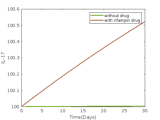
Figure 1 depicts the dynamics under rifampin administration, while figures 2 and 3 show the dynamics under dapsone and clofazimine administration, respectively. Average and 30th-day values of each compartment without control and with single drug intervention such as rifampin, dapsone, and clofazimine are presented in tables 10 and 11 respectively.

In all cases of single drug intervention, such as with drugs rifampin, dapsone and clofazimine, we observe from figures 1, 2, and 3 that the compartments susceptible cells $S(t)$ , infected cells $I(t)$ , and bacterial load $B(t)$ , as well as for IFN- $\gamma$ ( $I_{\gamma}(t)$ ), TNF- ${\alpha}$ ( $T_{\alpha}(t)$ ), IL-10 ( $I_{10}(t)$ ), and IL-12 ( $I_{12}(t)$ ), all show a decreasing trend compared to the scenario without drug intervention. Conversely, compartments IL-15 ( $I_{15}(t)$ ) and IL-17 ( $I_{17}(t)$ ), show an increasing trend.

The most significant reduction in susceptible cells is observed with dapsone, while the least reduction is observed with rifampin as a single drug intervention. Figure results for infected cells show consistency across all single drug interventions, but differences are noticeable in the values presented in tables 10 and 11. These tables indicate a decrease in infected cells, consistent with the trend observed for susceptible cells.

However, there is no discernible difference in the compartments bacterial load $B(t)$ , IFN- $\gamma$ ( $I_{\gamma}(t)$ ), TNF- ${\alpha}$ ( $T_{\alpha}(t)$ ), IL-10 ( $I_{10}(t)$ ), IL-12 ( $I_{12}(t)$ ), IL-15 ( $I_{15}(t)$ ), and IL-17 ( $I_{17}(t)$ ) when comparing the effects of all single drug interventions, as shown in both the figures 1 - 3 and tables 10, 11.

Figures 4, 5 and 6 illustrate the dynamics under combinations of drugs: rifampin & dapsone, clofazimin & dapsone and rifampin & clofazimine respectively. Average and 30th-day values of each compartment without control and with a two-drug combined intervention such as rifampin & dapsone, clofazimine & dapsone and rifampin & clofazimine are presented in tables 12 and 13 respectively.

In all cases of two-drug combination intervention, such as with combinations of rifampin and dapsone, dapsone and clofazimine, and rifampin and clofazimine, we observe from figures 4, 5, and 6 that the compartments exhibit trends similar to single drug intervention.

The most significant reduction in susceptible cells is observed with a combination of dapsone and clofazimine, while the least reduction is observed with a combination of rifampin and clofazimine as two-drug combined intervention. Results for infected cells show consistency across all combined two-drug interventions, but differences are noticeable in the values presented in tables 12 and 13. These tables indicate a decrease in infected cells, consistent with the trend observed for susceptible cells.

However, there is no discernible difference in the compartments bacterial load $B(t)$ , $I_{\gamma}(t)$ , $T_{\alpha}(t)$ , $I_{10}(t)$ , $I_{12}(t),$ $I_{15}(t)$ , and $I_{17}(t)$ when comparing the effects of all combined two-drug interventions, as shown in both figures 4 - 6 and table 12. However, there is a very slight increment in the compartment $I_{\gamma}(t)$ , and decrement in the compartments $T_{\alpha}(t)$ , $I_{10}(t)$ , and $I_{12}(t)$ with dapsone and clofazimine when comparing the effects of all combined two-drug interventions, as shown in table 13.

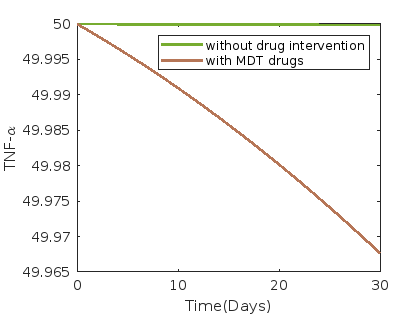
Figure 7 illustrates the dynamics under the administration of MDT drugs, comprising rifampin, clofazimine, and dapsone. Average and 30th-day values of each compartment without control and with MDT drug intervention such as rifampin, dapsone, and clofazimine are presented in table 14.

In case of MDT drugs (rifampin, clofazimine, and dapsone) intervention we observe from figure 7 that the compartments susceptible cells $S(t)$ , infected cells $I(t)$ , and bacterial load $B(t)$ , as well as for $I_{\gamma}(t)$ , $T_{\alpha}(t)$ , $I_{10}(t)$ , and $I_{12}(t)$ , show a decreasing trend compared to the scenario without drug intervention. Conversely, compartments $I_{15}(t)$ , and $I_{17}(t)$ , show an increasing trend.

Optimal drug values for individual drug administration, combination of two drugs, and MDT drug administration are presented in tables 7, 8, and 9 respectively.

Our findings indicate that current MDT drugs dosage for leprosy, as prescribed by physicians [15], are optimal according to our model.

Single Drug	Dosage monthly(in mg)	Initial drug dosage(in mg)	Optimal drug dosage(in mg)
Rifampin	600	20	19.999
Dapsone	3000	100	100.01
Clofazimine	300	10	10.001

Table 7: Dosage levels for individual drug administration for 30-days

Two Drugs	Monthly drug Dosage(in mg)	Combined dosage of two drugs(in mg)
Two Drugs	Monthly drug Dosage(in mg)	Initial	Optimal
Dapsone and Clofazimine	3000 + 300	100, 10	100.01, 9.999
Rifampin and Clofazimine	600 + 300	20, 10	19.999, 9.999
Rifampin and Dapsone	600 + 3000	20, 100	20.002, 99.999

Table 8: Dosage levels for combination of two drugs administration for 30-days

Three Drugs	Monthly drug Dosage(in mg)	MDT drug dosage (in mg)
Three Drugs	Monthly drug Dosage(in mg)	Initial	Optimal
Rifampin, Dapsone, Clofazimine	600+3000+300	20, 100, 10	20, 100, 10.001

Table 9: Dosage levels for the administration of all three drugs in MDT for 30-days

compartments	without drugs	with rifampin	with dapsone	with clofazimine
$S(t)$	519.999587	519.869137	518.629671	519.692631
$I(t)$	249.999579	249.936781	249.936732	249.936774
$B(t)$	2499.978250	2496.740464	2496.740464	2496.740464
$I_{\gamma}(t)$	49.988312	48.252862	48.252862	48.252862
$T_{\alpha}(t)$	49.999918	49.985089	49.985089	49.985089
$I_{10}(t)$	74.984018	72.659750	72.659750	72.659750
$I_{12}(t)$	124.998569	124.778566	124.778566	124.778566
$I_{15}(t)$	125.000643	125.079538	125.079538	125.079538
$I_{17}(t)$	100.001938	100.270343	100.270343	100.270343

Table 10: Average compartments values on individual administration of rifampin, dapsone, clofazimine over a 30-days period.

compartments	without drugs	with rifampin	with dapsone	with clofazimine
$S(t)$	519.999202	519.530281	513.249360	518.634813
$I(t)$	249.999186	249.877716	249.877398	249.877671
$B(t)$	2499.957950	2493.700671	2493.700671	2493.700671
$I_{\gamma}(t)$	49.977404	46.627260	46.627260	46.627260
$T_{\alpha}(t)$	49.999842	49.968988	49.968988	49.968988
$I_{10}(t)$	74.969104	70.522049	70.522049	70.522049
$I_{12}(t)$	124.997232	124.566354	124.566354	124.566354
$I_{15}(t)$	125.001243	125.139782	125.139782	125.139782
$I_{17}(t)$	100.003745	100.505891	100.505891	100.505891

Table 11: 30th-day compartments values on individual administration of rifampin, dapsone, clofazimine over a 30-days period.

compartments	without drugs	rifampin, dapsone	dapsone, clofazamine	clofazimine, rifampin
$S(t)$	519.999587	517.960166	515.850690	519.099803
$I(t)$	249.999579	249.936706	249.936623	249.936751
$B(t)$	2499.978250	2496.740464	2496.740464	2496.740464
$I_{\gamma}(t)$	49.988312	48.252862	48.252862	48.252862
$T_{\alpha}(t)$	49.999918	49.985089	49.985089	49.985089
$I_{10}(t)$	74.984018	72.659750	72.659750	72.659750
$I_{12}(t)$	124.998569	124.778566	124.778566	124.778566
$I_{15}(t)$	125.000643	125.079538	125.079538	125.079538
$I_{17}(t)$	100.001938	100.270343	100.270342	100.270343

Table 12: Average compartments values on combined administration of rifampin+dapsone, dapsone+clofazamine and clofazamine+rifampin over a 30-days period.

compartments	without drugs	rifampin, dapsone	dapsone, clofazamine	clofazimine, rifampin
$S(t)$	519.999202	509.865071	499.232056	515.630278
$I(t)$	249.999186	249.877226	249.876684	249.877519
$B(t)$	2499.957950	2493.700671	2493.700671	2493.700671
$I_{\gamma}(t)$	49.977404	46.627260	46.627261	46.627260
$T_{\alpha}(t)$	49.999842	49.968988	49.968987	49.968988
$I_{10}(t)$	74.969104	70.522049	70.522049	70.522049
$I_{12}(t)$	124.997232	124.566354	124.566354	124.566354
$I_{15}(t)$	125.001243	125.139782	125.139781	125.139782
$I_{17}(t)$	100.003745	100.505891	100.505890	100.505891

Table 13: 30th-day compartments values on combined administration of rifampin+dapsone, dapsone+clofazamine and clofazamine+rifampin over a 30-days period.

compartments	without drugs		rifampin, dapsone and clofazimine
compartments	Average	30th day	Average	30th day
$S(t)$	519.999587	519.999202	514.688830	493.397175
$I(t)$	249.999579	249.999186	249.936577	249.876385
$B(t)$	2499.978250	2499.957950	2496.740464	2493.700671
$I_{\gamma}(t)$	49.988312	49.977404	48.252862	46.627261
$T_{\alpha}(t)$	49.999918	49.999842	49.985089	49.968987
$I_{10}(t)$	74.984018	74.969104	72.659750	70.522049
$I_{12}(t)$	124.998569	124.997232	124.778566	124.566354
$I_{15}(t)$	125.000643	125.001243	125.079538	125.139781
$I_{17}(t)$	100.001938	100.003745	100.270342	100.505890

Table 14: Average and 30th day compartments values on MDT drug administration over a 30 days period.

5 Optimal Control studies incorporating second drug dosage

In this section, we introduce a delay into our model (1) - (11) to simulate a two-month duration for administering the drug, with the second dosage given 30 days after the first dosage based on tables 1 and 2 as per the clinical and medical guidelines. This model however can be extrapolated to real-administration scenario based on the WHO 2018 guidelines for Multi Drug therapy (MDT) consisting of drugs rifampin, dapsone and clofazimine with certain dosage administered every 30 days over a period of 12 months for the treatment of leprosy. The duration may vary based on whether it’s paucibacillary leprosy (6 months) or multibacillary leprosy (12 months). Request to kindly refer tables 1 and 2.

Motivated by the above now in our model (31) - (41), we introduce a delay of $\tau$ = 30 days.

We consider controls $D_{11}$ , $D_{21}$ , $D_{31}$ at $(t-\tau)$ for the first 30 days and controls $D_{12}$ , $D_{22}$ , $D_{32}$ associated with the next 30 days over a period of 60 days.

5.1 The Delay Model

The control set for this is given by

U=\Big{\{}D_{ij}(t)\ \big{|}\ D_{ij}(t)\in[0,D_{ij}max],1\leq i\leq 3,1\leq j\leq 2,t\in[0,T]\Big{\}},

and the revised objective function and the control system are provided as follows:
Cost functional:

\displaystyle\begin{split}\mathcal{J}_{min}\big{(}I,B,D_{11},D_{21},D_{31},D_{12},D_{22},D_{32}\big{)}\ &=\int_{0}^{T}\Big{(}I(t)+B(t)+P(D^{2}_{11}(t-\tau)+D^{2}_{12}(t))\\ \ &+Q(D^{2}_{21}(t-\tau)+D^{2}_{22}(t))+R(D_{31}^{2}(t-\tau)+D_{32}^{2}(t))\Big{)}dt\end{split}

(30)

Control system:

$\displaystyle\frac{dc_{1}}{dt}\$	$\displaystyle=\ \frac{D_{11}(t-\tau)+D_{21}(t-\tau)+D_{31}(t-\tau)}{V_{1}}+\frac{D_{12}(t)+D_{2}(t)+D_{3}(t)}{V_{1}}\ -\big{(}k_{12}+k_{1}\big{)}c_{1}$	(31)
$\displaystyle\frac{dc_{2}}{dt}\$	$\displaystyle=\ k_{12}\frac{V_{1}}{V_{2}}c_{1}\ -k_{2}c_{2}$	(32)
$\displaystyle\frac{dS}{dt}\$	$\displaystyle=\ \omega\ -\beta SB-\gamma S-\mu_{1}S-(\mu_{d_{1}}+\mu_{d_{2}}+\mu_{d_{3}})c_{1}(t-\tau-\tau_{d})S-(\mu_{d_{1}}+\mu_{d_{2}}+\mu_{d_{3}})c_{1}(t-\tau_{d})S$	(33)
$\displaystyle\frac{dI}{dt}\$	$\displaystyle=\ \beta SB\ -\delta I-\mu_{1}I-(\eta k_{d_{1}}+\eta k_{d_{2}}+\eta k_{d_{3}})\cdot(c_{2}-C_{min})\cdot H\left[(c_{2}-C_{min})\right]\cdot I$	(34)
$\displaystyle\frac{dB}{dt}\$	$\displaystyle=\ \alpha I\ -yB-\mu_{2}B-(k_{d_{1}}+k_{d_{2}}+k_{d_{3}})\cdot(c_{2}-C_{min})\cdot H\left[(c_{2}-C_{min})\right]\cdot B$	(35)
$\displaystyle\frac{dI_{\gamma}}{dt}\$	$\displaystyle=\ \alpha_{I_{\gamma}}I\ -\left[\delta_{T_{\alpha}}^{I_{\gamma}}T_{\alpha}+\delta_{I_{12}}^{I_{\gamma}}I_{12}+\delta_{I_{15}}^{I_{\gamma}}I_{15}+\delta_{I_{17}}^{I_{\gamma}}I_{17}\right]I-\mu_{I_{\gamma}}\big{(}I_{\gamma}-Q_{I_{\gamma}}\big{)}$	(36)
$\displaystyle\frac{dT_{\alpha}}{dt}\$	$\displaystyle=\ \beta_{T_{\alpha}}I_{\gamma}I\ -\mu_{T_{\alpha}}\big{(}T_{\alpha}-Q_{T_{\alpha}}\big{)}$	(37)
$\displaystyle\frac{dI_{10}}{dt}\$	$\displaystyle=\ \alpha_{I_{10}}I\ -\delta_{I_{\gamma}}^{I_{10}}I_{\gamma}-\mu_{I_{10}}\big{(}I_{10}-Q_{I_{10}}\big{)}$	(38)
$\displaystyle\frac{dI_{12}}{dt}\$	$\displaystyle=\ \beta_{I_{12}}I_{\gamma}I\ -\mu_{I_{12}}\big{(}I_{12}-Q_{I_{12}}\big{)}$	(39)
$\displaystyle\frac{dI_{15}}{dt}\$	$\displaystyle=\ \beta_{I_{15}}I_{\gamma}I\ -\mu_{I_{15}}\big{(}I_{15}-Q_{I_{15}}\big{)}$	(40)
$\displaystyle\frac{dI_{17}}{dt}\$	$\displaystyle=\ \beta_{I_{17}}I_{\gamma}I\ -\mu_{I_{17}}\big{(}I_{17}-Q_{I_{17}}\big{)}$	(41)

Here, the Lagrangian is the integrand of the cost functional (30) and is given by

\displaystyle\begin{split}L(I,B,D_{11},D_{21},D_{31},D_{12},D_{22},D_{32})\ &=I(t)+B(t)+P(D^{2}_{11}(t-\tau)+D^{2}_{12}(t))\\ \ &+Q(D^{2}_{21}(t-\tau)+D^{2}_{22}(t))+R(D_{31}^{2}(t-\tau)+D_{32}^{2}(t))\end{split}

(42)

The set of admissible solutions for the above optimal control problem will be

\Omega=\Big{\{}(I,B,D_{11},D_{21},D_{31},D_{12},D_{22},D_{32})\ \big{|}I,B\ satisfy\ (\ref{sec5equ1})-(\ref{sec5equ11})\ \forall(D_{11},D_{21},D_{31},D_{12},D_{22},D_{32})\in U\Big{\}}.

The existence of optimal control can be shown similarly as in section 4.
The Hamiltonian of the control system (31) - (41) is as follows

\displaystyle\begin{split}\mathcal{H}(I,B,D_{11},D_{21},D_{31},D_{12},D_{22},D_{32},\lambda)&=L(I,B,D_{11},D_{21},D_{31},D_{12},D_{22},D_{32})+\lambda_{1}\frac{dc_{1}}{dt}+\lambda_{2}\frac{dc_{2}}{dt}\\ \ &+\lambda_{3}\frac{dS}{dt}+\lambda_{4}\frac{dI}{dt}+\lambda_{5}\frac{dB}{dt}+\lambda_{6}\frac{dI_{\gamma}}{dt}+\lambda_{7}\frac{dT_{\alpha}}{dt}+\lambda_{8}\frac{dI_{10}}{dt}\\ \ &+\lambda_{9}\frac{dI_{12}}{dt}+\lambda_{10}\frac{dI_{15}}{dt}+\lambda_{11}\frac{dI_{17}}{dt}\end{split}

(43)

where $\lambda=(\lambda_{1},\lambda_{2},\lambda_{3},\lambda_{4},\lambda_{5},\lambda_{6},\lambda_{7},\lambda_{8},\lambda_{9},\lambda_{10},\lambda_{11})$ is co-state variable or adjoint vector.

Since we have $D^{*}=(D_{11}^{*},D_{12}^{*},D_{21}^{*},D_{22}^{*},D_{31}^{*},D_{32}^{*})$ and $X^{*}=(x_{1},x_{2},x_{3},x_{4},x_{5},x_{6},x_{7},x_{8},x_{9},x_{10},x_{11})$ as optimal control and state variable respectively, using Pontryagin maximum principle there exists an optimal co-state variable say $\lambda^{*}$ which satisfies the canonical equation

\frac{d\lambda_{j}}{dt}=-\frac{\partial\mathcal{H}(X^{*},D^{*},\lambda^{*})}{\partial x_{j}}

(44)

Using the above equation we get the below system of ODE’s for co-state variables as follows

$\displaystyle\frac{d\lambda_{1}}{dt}$	$\displaystyle=(k_{12}+k_{1})\lambda_{1}-k_{12}\left(\frac{V_{1}}{V_{2}}\right)\lambda_{2}+2(\mu_{d_{1}}+\mu_{d_{2}}+\mu_{d_{3}})S\lambda_{3}$	(45)
$\displaystyle\frac{d\lambda_{2}}{dt}$	$\displaystyle=k_{2}\lambda_{2}+\eta(k_{d_{1}}+k_{d_{2}}+k_{d_{3}})H[(c_{2}-c_{min})]\cdot I\lambda_{4}+(k_{d_{1}}+k_{d_{2}}+k_{d_{3}})H[(c_{2}-c_{min})]\cdot B\lambda_{5}$	(46)
$\displaystyle\frac{d\lambda_{3}}{dt}$	$\displaystyle=\big{(}\beta B+\mu_{1}+\gamma+(\mu_{d_{1}}+\mu_{d_{2}}+\mu_{d_{3}})c_{1}(t-\tau-\tau_{d})+(\mu_{d_{1}}+\mu_{d_{2}}+\mu_{d_{3}})c_{1}(t-\tau_{d})\big{)}\lambda_{3}-\beta B\lambda_{4}$	(47)
$\displaystyle\begin{split}\frac{d\lambda_{4}}{dt}&=\big{(}\delta+\mu_{1}+(\eta k_{d_{1}}+\eta k_{d_{2}}+\eta k_{d_{3}})(c_{2}-C_{min})H[(c_{2}-C_{min})]\big{)}\lambda_{4}-\alpha\lambda_{5}-\alpha_{I_{\gamma}}\lambda_{6}\\ \ &+\left(\delta_{T_{\alpha}}^{I_{\gamma}}T_{\alpha}+\delta_{I_{12}}^{I_{\gamma}}I_{12}+\delta_{I_{15}}^{I_{\gamma}}I_{15}+\delta_{I_{17}}^{I_{\gamma}}I_{17}\right)\lambda_{6}+\beta_{T_{\alpha}}I_{\gamma}\lambda_{7}-\alpha_{I_{10}}\lambda_{8}-\beta_{I_{12}}I_{\gamma}\lambda_{9}-\beta_{I_{15}}I_{\gamma}\lambda_{10}-\beta_{I_{17}}I_{\gamma}\lambda_{11}-1\end{split}$		(48)
$\displaystyle\frac{d\lambda_{5}}{dt}$	$\displaystyle=\beta S\lambda_{3}-\beta S\lambda_{4}+\big{(}y+\mu_{2}+(k_{d_{1}}+k_{d_{2}}+k_{d_{3}})(c_{2}-C_{min})H[(c_{2}-C_{min})]\big{)}\lambda_{5}-1$	(49)
$\displaystyle\frac{d\lambda_{6}}{dt}$	$\displaystyle=\mu_{I_{\gamma}}\lambda_{6}-\beta_{T_{\alpha}}I\lambda_{7}+\delta_{I_{10}}^{I_{\gamma}}I\lambda_{8}-\beta_{I_{12}}I\lambda_{9}-\beta_{I_{15}}I\lambda_{10}-\beta_{I_{17}}I\lambda_{11}$	(50)
$\displaystyle\frac{d\lambda_{7}}{dt}$	$\displaystyle=\delta_{T_{\alpha}}^{I_{\gamma}}I\lambda_{6}+\mu_{T_{\alpha}}\lambda_{7}$	(51)
$\displaystyle\frac{d\lambda_{8}}{dt}$	$\displaystyle=\mu_{I_{10}}\lambda_{8}$	(52)
$\displaystyle\frac{d\lambda_{9}}{dt}$	$\displaystyle=\delta_{I_{12}}^{I_{\gamma}}I\lambda_{6}+\mu_{I_{12}}\lambda_{9}$	(53)
$\displaystyle\frac{d\lambda_{10}}{dt}$	$\displaystyle=\delta_{I_{15}}^{I_{\gamma}}I\lambda_{6}+\mu_{I_{15}}\lambda_{10}$	(54)
$\displaystyle\frac{d\lambda_{11}}{dt}$	$\displaystyle=\delta_{I_{17}}^{I_{\gamma}}I\lambda_{6}+\mu_{I_{17}}\lambda_{11}$	(55)

Now we use $Newton^{\prime}s\ Gradient\ method$ from [22] to obtain the optimal value of the controls. For this recursive formula is employed to update the control at each step of the numerical simulation as follows

\displaystyle D_{ij}^{k+1}(t)=D_{ij}^{k}(t)+\theta_{k}d_{k}

(56)

Here, $D_{ij}^{k}(t)$ represents the control value at the $k^{th}$ iteration at a given time $t$ , $d_{k}$ signifies the direction, and $\theta_{k}$ denotes the step size. The direction $d_{k}$ can be evaluated as negative of gradient of the objective function i.e $d_{k}=-g_{ij}(D_{ij}^{k})$ ,where $g_{ij}(D_{ij}^{k})=\frac{\partial\mathcal{H}}{\partial D_{ij}}\big{|}_{D_{ij}^{k}(t)}$ as mentioned in[22].The step size $\theta_{k}$ is determined at each iteration using a linear search technique aimed at minimizing the Hamiltonian, $\mathcal{H}$ .Therefore (56) can become as

\displaystyle D_{ij}^{k+1}(t)=D_{ij}^{k}(t)-\theta_{k}\frac{\partial\mathcal{H}}{\partial D_{ij}}\Big{|}_{D_{ij}^{k}(t)}

(57)

To implement the aforementioned approach, we need to compute the gradient for each control, denoted as $g_{ij}(D_{ij}^{k})$ , which are listed as follows

	$\displaystyle g_{11}(D_{11})\$	$\displaystyle=2PD_{11}(t-\tau)+\frac{\lambda_{1}}{V_{1}}$
	$\displaystyle g_{12}(D_{12})\$	$\displaystyle=2PD_{12}(t)+\frac{\lambda_{1}}{V_{1}}$
	$\displaystyle g_{21}(D_{21})\$	$\displaystyle=2QD_{21}(t-\tau)+\frac{\lambda_{1}}{V_{1}}$
	$\displaystyle g_{22}(D_{22})\$	$\displaystyle=2QD_{22}(t)+\frac{\lambda_{1}}{V_{1}}$
	$\displaystyle g_{31}(D_{31})\$	$\displaystyle=2RD_{31}(t-\tau)+\frac{\lambda_{1}}{V_{1}}$
	$\displaystyle g_{32}(D_{32})\$	$\displaystyle=2RD_{32}(t)+\frac{\lambda_{1}}{V_{1}}$

5.2 Numerical simulations

Here, we employ the parameter values, initial conditions, and numerical simulation methods identical to those used in section 4.2. Additionally, we introduce one extra control associated with each drug, with a delay of $\tau=30$ days. Therefore, the values of weights associated with these controls remain the same as in section 4.2. We proceed to numerically simulate the populations of $c_{1},$ $c_{2},$ $S,$ $I,$ and $B$ along with cytokines levels, employing single, double and triple control interventions of MDT for 60 days with a delay of 30 days for second dosage.

5.3 Findings

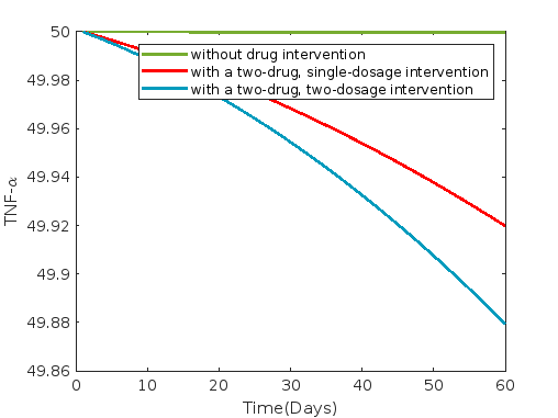
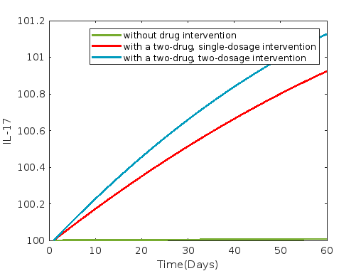
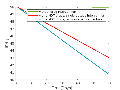
In this section, we analyze the results from the simulations described earlier. Figures 8 - 14 depict the dynamics of the $S$ , $I$ , $B$ , $I_{\gamma}$ , $T_{\alpha}$ , $I_{10}$ , $I_{12}$ , $I_{15}$ , and $I_{17}$ compartments in our model (33)–(41). Additionally, these figures illustrate the control flow associated with under different drug administration scenarios over a 60-day period with a single delay of 30 days. Each panel represents a compartment and compares its dynamics without drug intervention, with single dosgae drug interventions and two dosage drug interventions.

Figure 8 depicts the dynamics under rifampin administration, while figures 9 and 10 show the dynamics under dapsone and clofazimine administration, respectively. Average and 60th-day values of each compartment without control and with single drug intervention such as rifampin, dapsone, and clofazimine are presented in tables 18 and 19 respectively, with a 30-day delay for second dosage.

In all instances of single drug intervention, involving the administration of rifampin, dapsone, and clofazimine, it is evident from figures 8, 9, and 10 that various compartments, including susceptible cells $S(t)$ , infected cells $I(t)$ , and bacterial load $B(t)$ , as well as $I_{\gamma}(t)$ , $T_{\alpha}(t)$ , $I_{10}(t)$ , and $I_{12}(t)$ , exhibit a decreasing trend when compared to scenarios without drug intervention and delay. Conversely, compartments $I_{15}(t)$ and $I_{17}(t)$ demonstrate an increasing trend.

Dapsone exhibits the most substantial reduction in both susceptible and infected cells whereas rifampin shows the least reduction when administered as a single drug intervention.

The results from the figures 8, 9, and 10 depictit that the compartments bacterial load, IFN- $\gamma$ , TNF- ${\alpha}$ , IL-10, IL-12, IL-15, and IL-17 show consistency across all single drug interventions. However, differences are noticeable in the values presented in tables 10 and 11. Additionally, these tables clearly indicate a reduction in infected cells.

From tables 10 and 11, 18, 19 it is evident that, similar to susceptible and infected cells, dapsone is also more effective in reducing bacterial load, TNF- ${\alpha}$ , IL-10, and IL-12, whereas rifampin shows the least reduction when administered as a single drug intervention.

IFN- $\gamma$ experiences the most significant reduction with rifampin and the least with dapsone. Additionally, the increment of IL-15 and IL-17 is greater with rifampin and least with dapsone.

Figures 11, 12 and 13 illustrate the dynamics under combinations of two drugs: rifampin and dapsone, clofazimine and dapsone, and rifampin and clofazimine, respectively. Average and 60th-day values of each compartment without control and with a two-drug combined intervention such as rifampin and dapsone, clofazimine and dapsone, and rifampin and clofazimine are presented in tables 20 and 21 respectively, where a 30-day delay is incorporated for second dosage.

In all instances of two-drug combination intervention, involving the administration of drug combinations such as rifampin and dapsone, dapsone and clofazimine, and rifampin and clofazimine, it is evident from figures 11, 12, and 13 that various compartments, including susceptible cells $S(t)$ , infected cells $I(t)$ , and bacterial load $B(t)$ , as well as $I_{\gamma}(t)$ , $T_{\alpha}(t)$ , $I_{10}(t)$ , and $I_{12}(t)$ , exhibit a decreasing trend when compared to scenarios without drug intervention and delay. Conversely, compartments $I_{15}(t)$ and $I_{17}(t)$ demonstrate an increasing trend.

The two-drug combination of dapsone and clofazimine exhibits the most substantial reduction in both susceptible and infected cells, whereas the two-drug combination of rifampin and clofazimine shows the least reduction when administered as a two-drug intervention.

The results from figures 11, 12, and 13 depicting the compartments bacterial load, IFN- $\gamma$ , TNF- ${\alpha}$ , IL-10, IL-12, IL-15, and IL-17, show consistency across all two-drug interventions. However, differences are noticeable in the values presented in tables 20 and 21. Additionally, these tables clearly indicate a reduction in infected cells.

From tables 20 and 21, it is evident that, similar to susceptible and infected cells, dapsone and clofazimine is also more effective in reducing bacterial load, TNF- ${\alpha}$ , IL-10, and IL-12, whereas rifampin and clofazimine shows the least reduction when administered as a two-drug intervention.

IFN- $\gamma$ experiences the most significant reduction with rifampin and clofazimine, and the least with dapsone and clofazimine. Additionally, the increment of IL-15 and IL-17 is greater with rifampin and clofazimine, and less with dapsone and clofazimine in two-drug combination.

Figure 14 illustrates the dynamics under the administration of MDT drugs, comprising rifampin, clofazimine, and dapsone.

Average and 60th-day values of each compartment without control and with MDT drug intervention such as rifampin, dapsone, and clofazimine are presented in table 22, where a 30-day delay is incorporated for second drug dosage.

In case of MDT drug (rifampin, clofazimine, and dapsone) interventions, we observe from figure 14 that the compartments susceptible cells $S(t)$ , infected cells $I(t)$ , and bacterial load $B(t)$ , as well as for $I_{\gamma}(t)$ , $T_{\alpha}(t)$ , $I_{10}(t)$ , and $I_{12}(t)$ , show a decreasing trend compared to the scenarios without drug intervention and delay. Conversely, compartments $I_{15}(t)$ , and $I_{17}(t)$ , show an increasing trend.

Optimal drug values for individual drug administration, combination of two drugs, and MDT drug administration with two dosages at the first day and next at the 31th day over a 60-day period are presented in tables 15, 16 and 17, respectively.

Single Drug	Monthly dosage(mg)	First dosage for 60 days(mg)		Second dosage at 31th-day(mg)
Single Drug	Monthly dosage(mg)	Initial	Optimal	Initial	Optimal
Rifampin	600	10	10	20	20.013
Dapsone	3000	50	50.002	100	100.009
Clofazimine	300	5	5.001	10	10.005

Table 15: Dosage levels for individual drug administration for 60-days with delay of 30 days for second drug dosage

Two Drugs	Monthly dosage(mg)	1st dose for 60 days(mg)		2nd dose at 31th-day(mg)
Two Drugs	Monthly dosage(mg)	Initial(mg)	Optimal(mg)	Initial(mg)	Optimal(mg)
Rifampin and Dapsone	600 + 3000	10, 50	10.001, 50.001	20, 100	20.049, 99.949
Dapsone and Clofazimine	3000 + 300	50, 5	49.998, 5.00	100, 10	99.785, 9.996
Rifampin and Clofazimine	600 + 300	10, 5	10.001, 4.999	20, 10	19.994, 10.037

Table 16: Dosage levels for combination of two drugs administration for 60-days with delay of 30 days for second drug dosage

Three Drugs	Monthly dosage(mg)	1st dose for 60 days(mg)		2nd dose at 31th-day(mg)
Three Drugs	Monthly dosage(mg)	Initial(mg)	Optimal(mg)	Initial(mg)	Optimal(mg)
MDT	600+3000+300	10, 50, 5	10.001, 50.002, 5.001	20, 100, 10	19.872, 99.985, 9.939

Table 17: Drug dosage levels for three drugs administrtion in MDT for 60-days with delay of 30 days for second drug dosage

compartments	without drugs	with rifampin	with dapsone	with clofazimine
$S(t)$	519.999174	516.754182	465.067903	508.975006
$I(t)$	249.999158	249.830213	249.813952	249.827797
$B(t)$	2499.956501	2491.320879	2491.320869	2491.320878
$I_{\gamma}(t)$	49.976625	45.368405	45.368540	45.368425
$T_{\alpha}(t)$	49.999836	49.948694	49.948685	49.948693
$I_{10}(t)$	74.968042	68.999333	68.999308	68.999329
$I_{12}(t)$	124.997136	124.380295	124.380272	124.380292
$I_{15}(t)$	125.001285	125.138320	125.138267	125.138313
$I_{17}(t)$	100.003874	100.632488	100.632426	100.632479

Table 18: Average compartments values on administration of two dosages of rifampin, dapsone, clofazimine over 60-days period with second dosage administered on 31st day.

compartments	without drugs	with rifampin	with dapsone	with clofazimine
$S(t)$	519.998376	513.676795	416.540017	498.630305
$I(t)$	249.998344	249.664919	249.620094	249.658183
$B(t)$	2499.914452	2482.950034	2482.949997	2482.950028
$I_{\gamma}(t)$	49.954030	40.931982	40.932477	40.932056
$T_{\alpha}(t)$	49.999677	49.882312	49.882282	49.882308
$I_{10}(t)$	74.937158	63.540457	63.540364	63.540443
$I_{12}(t)$	124.994367	123.738840	123.738757	123.738828
$I_{15}(t)$	125.002524	125.164927	125.164738	125.164899
$I_{17}(t)$	100.007615	101.115553	101.115334	101.115521

Table 19: 60th-day compartments values on administration of two dosages of rifampin, dapsone, clofazimine over 60-days period with second dosage administered on 31st day.

compartments	without drugs	rifampin, dapsone	dapsone, clofazamine	clofazimine, rifampin
$S(t)$	519.999174	439.854184	370.958732	483.892621
$I(t)$	249.999158	249.805823	249.782830	249.819934
$B(t)$	2499.956501	2491.320864	2491.320850	2491.320873
$I_{\gamma}(t)$	49.976625	45.368608	45.368805	45.368490
$T_{\alpha}(t)$	49.999836	49.948681	49.948669	49.948689
$I_{10}(t)$	74.968042	68.999295	68.999257	68.999317
$I_{12}(t)$	124.997136	124.380260	124.380225	124.380280
$I_{15}(t)$	125.001285	125.138240	125.138162	125.138287
$I_{17}(t)$	100.003874	100.632395	100.632304	100.632449

Table 20: Average compartments values on administration of two dosages of rifampin & dapsone, dapsone & clofazamine and clofazamine & rifampin over 60-days period with second dosage administered on 31st day.

compartments	without drugs	rifampin, dapsone	dapsone, clofazamine	clofazimine, rifampin
$S(t)$	519.998376	371.691390	258.561537	451.132838
$I(t)$	249.998344	249.598166	249.538020	249.636439
$B(t)$	2499.914452	2482.949978	2482.949926	2482.950010
$I_{\gamma}(t)$	49.954030	40.932724	40.933426	40.932295
$T_{\alpha}(t)$	49.999677	49.882267	49.882224	49.882293
$I_{10}(t)$	74.937158	63.540317	63.540186	63.540398
$I_{12}(t)$	124.994367	123.738715	123.738597	123.738787
$I_{15}(t)$	125.002524	125.164643	125.164375	125.164808
$I_{17}(t)$	100.007615	101.115224	101.114913	101.115415

Table 21: 60th-day compartments values on administration of two dosages of rifampin & dapsone, dapsone & clofazamine and clofazamine & rifampin over 60-days period with second dosage administered on 31st day.

compartments	without drugs		rifampin, dapsone and clofazimine
compartments	Average	60th day	Average	60th day
$S(t)$	519.999174	519.998376	338.956016	211.188822
$I(t)$	249.999158	249.998344	249.771687	249.509958
$B(t)$	2499.956501	2499.914452	2491.320842	2482.949901
$I_{\gamma}(t)$	49.976625	49.954030	45.368903	40.933768
$T_{\alpha}(t)$	49.999836	49.999677	49.948662	49.882203
$I_{10}(t)$	74.968042	74.937158	68.999239	63.540122
$I_{12}(t)$	124.997136	124.994367	124.380208	123.738539
$I_{15}(t)$	125.001285	125.002524	125.138123	125.164245
$I_{17}(t)$	100.003874	100.007615	100.632259	101.114762

Table 22: Average and 60th day compartments values on administration of two dosages of all MDT drug over 60-days period with second dosage administered on 31st day.

6 Discussions and Conclusions

The present work is novel and first of its kind dealing with the dynamics dealing with the levels of crucial bio-markers that are involved in Type 1 lepra reaction and their quantitative correlations with the MDT drugs along with the optimal dosages.

We have explored these correlations for administration of drugs in two dosages for the MDT drugs namely rifampin, clofazimine & dapsone with respect to individual and combined implementation. These scenarios have been numerically simulated and the findings have been extensively discussed. These study also explored the optimal drug dosages for administration and it was found out that the optimal drug dosage of the MDT drugs found through these optimal control studies and the dosage prescribed as per WHO guidelines are almost the same.

In conclusion we suggest that the present research work can be extrapolated to real-administration scenario based on the WHO 2018 guidelines for Multi Drug therapy (MDT) consisting of drugs rifampin, dapsone and clofazimine with certain dosage administered every 30 days over a period of 12 months for the treatment of lepra type I and type II reactions. The duration may vary based on whether it’s paucibacillary leprosy (6 months) or multibacillary leprosy (12 months).

Also this study can be of important help to the clinician in early detection of the leprosy and avoid and control the disease from going to Lepra reactions and help in averting major damages.

Funding

This research was supported by Council of Scientific and Industrial Research (CSIR) under project grant - Role and Interactions of Biological Markers in Causation of Type1/Type 2 Lepra Reactions: A In Vivo Mathematical Modelling with Clinical Validation (Sanction Letter No. 25(0317)/20/EMR-II).

Data Availability Statement (DAS)

We do not analyse or generate any datasets, because our work proceeds within a theoretical and mathematical approach.

Declarations

The authors declare no Conflict of Interest for this research work.

Ethics Statement

This research did not require any ethical approval.

Acknowledgments

The authors dedicate this paper to the founder chancellor of SSSIHL, Bhagawan Sri Sathya Sai Baba. The corresponding author also dedicates this paper to his loving elder brother D. A. C. Prakash who still lives in his heart.

References

[1] WHO “Leprosy”, 2023 URL: https://www.who.int/news-room/fact-sheets/detail/leprosy
[2] WHO “Number of new Leprosy cases in 2022”, 2024 URL: https://apps.who.int/neglected_diseases/ntddata/leprosy/leprosy.html
[3] M Lechat et al. “An epidemetric model of leprosy” In Bulletin of the World Health Organization, 1974
[4] Michel F Lechat et al. “Simulation of vaccination and resistance in leprosy using an epidemiometric model” In Int. J. Lepr, 1985
[5] David J Blok, Sake J Vlas, Egil AJ Fischer and Jan Hendrik Richardus “Mathematical modelling of leprosy and its control” In Advances in Parasitology Elsevier, 2015
[6] LAH Giraldo et al. “Multibacillary and paucibacillary leprosy dynamics: a simulation model including a delay” In Appl Math Sci, 2018
[7] S Ghosh et al. “Mathematical Modeling and Control of the Cell Dynamics in Leprosy” In Computational Mathematics and Modeling Springer, 2021
[8] Rudolf Virchow “Die krankhaften Geschwülste: 30 Vorlesungen, geh. während d. Wintersemesters 1862-1863 an d. Univ. zu Berlin” Hirschwald, 1865
[9] Yuqian Luo et al. “Host-related laboratory parameters for leprosy reactions” In Frontiers in Medicine Frontiers Media SA, 2021
[10] Leyla Bilik, Betul Demir and Demet Cicek “Leprosy reactions” In Hansen’s Disease-The Forgotten and Neglected Disease, 2019
[11] Rosane B Oliveira et al. “Cytokines and Mycobacterium leprae induce apoptosis in human Schwann cells” In Journal of Neuropathology & Experimental Neurology American Association of Neuropathologists, Inc., 2005
[12] Olabisi Ojo, Diana L Williams, Linda B Adams and Ramanuj Lahiri “Mycobacterium leprae transcriptome during in vivo growth and ex vivo stationary phases” In Frontiers in cellular and infection microbiology Frontiers, 2022
[13] Dinesh Nayak, Anamalamudi Vilvanathan Sangeetha and Dasu Krishna Kiran Vamsi “A study of qualitative correlations between crucial bio-markers and the optimal drug regimen of Type I lepra reaction: A deterministic approach” In Computational and Mathematical Biophysics De Gruyter, 2023
[14] D Nayak et al. “A comprehensive and detailed within-host modeling study involving crucial biomarkers and optimal drug regimen for type i lepra reaction: A deterministic approach” In Computational and Mathematical Biophysics, 2023
[15] Mayra BC Maymone et al. “Leprosy: Treatment and management of complications” In Journal of the American Academy of Dermatology Elsevier, 2020
[16] D. A. “Optimizing drug regimens in cancer chemother- apy by an efficacy–toxicity mathematical model” In Computers and Biomed- ical Research Academic Press, 2000
[17] KD Tripathi “Essentials of medical pharmacology” JP Medical Ltd, 2013
[18] W.. world “Heaviside step function” URL: https://mathworld.wolfram.com/HeavisideStepFunction.html
[19] A Boyarsky “On the existence of optimal controls for nonlinear systems” In Journal of Optimization Theory and Applications Plenum Press New York, NY, USA, 1976
[20] Michael McAsey, Libin Mou and Weimin Han “Convergence of the forward-backward sweep method in optimal control” In Computational Optimization and Applications Springer, 2012
[21] Daniel Liberzon “Calculus of variations and optimal control theory: a concise introduction” Princeton university press, 2011
[22] Ernest R Edge and William Francis Powers “Function-space quasi-Newton algorithms for optimal control problems with bounded controls and singular arcs” In Journal of Optimization Theory and Applications Springer, 1976
[23] Kang-Ling Liao, Xue-Feng Bai and Avner Friedman “The role of CD200–CD200R in tumor immune evasion” In Journal of theoretical biology Elsevier, 2013
[24] Han-Seop Kim et al. “Schwann cell precursors from human pluripotent stem cells as a potential therapeutic target for myelin repair” In Stem cell reports Elsevier, 2017
[25] Song-Hyo Jin, Sung-Kwan An and Seong-Beom Lee “The formation of lipid droplets favors intracellular Mycobacterium leprae survival in SW-10, non-myelinating Schwann cells” In PLoS neglected tropical diseases Public Library of Science San Francisco, CA USA, 2017
[26] Louis Levy and JI Baohong “The mouse foot-pad technique for cultivation of Mycobacterium leprae” In Leprosy review 77.1, 2006, pp. 5–24
[27] International Leprosy Association “International Journal of Leprosy and Other Mycobacterial Diseases”, 2020
[28] Usman Pagalay “A mathematical model for interaction macrophages, T Lymphocytes and Cytokines at infection of mycobacterium tuberculosis with age influence” In International Journal of Science and Technology IEESE Institute of Excellent Engineer Science, 2014
[29] Bo Su, Wen Zhou, KS Dorman and DE Jones “Mathematical modelling of immune response in tissues” In Computational and Mathematical Methods in Medicine Taylor & Francis, 2009
[30] Kian Talaei et al. “A mathematical model of the dynamics of cytokine expression and human immune cell activation in response to the pathogen staphylococcus aureus” In Frontiers in Cellular and Infection Microbiology Frontiers, 2021
[31] Renee Brady et al. “Personalized Mathematical Model Predicting Endotoxin-Induced Inflammatory Responses in Young Men” In arXiv preprint arXiv:1609.01570, 2016
[32] Mirjam I Bakker et al. “Prevention of leprosy using rifampicin as chemoprophylaxis” In The American journal of tropical medicine and hygiene American Society of Tropical MedicineHygiene, 2005
[33] Selma Regina Penha Silva Cerqueira et al. “The influence of leprosy-related clinical and epidemiological variables in the occurrence and severity of COVID-19: A prospective real-world cohort study” In PLoS neglected tropical diseases Public Library of Science San Francisco, CA USA, 2021