This paper was converted on www.awesomepapers.org from LaTeX by an anonymous user.
Want to know more? Visit the Converter page.

11institutetext: W. Bao 22institutetext: Department of Mathematics, National University of Singapore, Singapore 119076
Fax: +65-6779-5452, Tel.: +65-6516-2765,
URL: https://blog.nus.edu.sg/matbwz/
22email: [email protected]
Y. Li
33institutetext: Department of Mathematics, National University of Singapore, Singapore 119076
33email: [email protected]

A structure-preserving parametric finite element method for geometric flows with anisotropic surface energy

Weizhu Bao    Yifei Li
(Received: date / Accepted: date)
Abstract

We propose and analyze structure-preserving parametric finite element methods (SP-PFEM) for evolution of a closed curve under different geometric flows with arbitrary anisotropic surface energy γ(𝒏)\gamma(\boldsymbol{n}) for 𝒏𝕊1\boldsymbol{n}\in\mathbb{S}^{1} representing the outward unit normal vector. By introducing a novel surface energy matrix 𝑮k(𝒏)\boldsymbol{G}_{k}(\boldsymbol{n}) depending on γ(𝒏)\gamma(\boldsymbol{n}) and the Cahn-Hoffman 𝝃\boldsymbol{\xi}-vector as well as a nonnegative stabilizing function k(𝒏):𝕊1k(\boldsymbol{n}):\ \mathbb{S}^{1}\to\mathbb{R}, which is a sum of a symmetric positive definite matrix and an anti-symmetric matrix, we obtain a new geometric partial differential equation and its corresponding variational formulation for the evolution of a closed curve under anisotropic surface diffusion. Based on the new weak formulation, we propose a parametric finite element method for the anisotropic surface diffusion and show that it is area conservation and energy dissipation under a very mild condition on γ(𝒏)\gamma(\boldsymbol{n}). The SP-PFEM is then extended to simulate evolution of a close curve under other anisotropic geometric flows including anisotropic curvature flow and area-conserved anisotropic curvature flow. Extensive numerical results are reported to demonstrate the efficiency and unconditional energy stability as well as good mesh quality property of the proposed SP-PFEM for simulating anisotropic geometric flows.

Keywords:
geometric flows parametric finite element method anisotropy surface energy structure-preserving area conservation energy-stable
MSC:
65M60, 65M12, 35K55, 53C44
journal: Numer. Math.

1 Introduction

Anisotropic surface energy along surface/interface is ubiquitous in solids and materials science due to the lattice orientational difference gurtin2002interface ; Cahn94 . It thus generates anisotropic evolution process of interface/surface (or geometric flows with anisotropic surface energy) in material sciences Sutton95 ; Thompson12 ; jiang2012 , imaging sciences niessen1997general ; clarenz2000anisotropic ; dolcetta2002area , and computational geometry wang2015sharp ; Cahn94 ; deckelnick2005computation . In fact, anisotropic geometric flows have significant and broader applications in materials science, solid-state physics and computational geometry, such as grain boundary growth barrett2010finite , foam bubble/film shen2004direct , surface phase formation Ye10a , epitaxial growth Fonseca14 ; gurtin2002interface , heterogeneous catalysis randolph2007controlling , solid-state dewetting Thompson12 ; bao2017parametric ; https://doi.org/10.48550/arxiv.2012.11404 , computational graphics niessen1997general ; clarenz2000anisotropic ; dolcetta2002area .

Assume Γ\Gamma be a closed curve in two dimensions (2D) associated with a given anisotropic surface energy γ(𝒏)\gamma(\boldsymbol{n}), where 𝒏=(n1,n2)T𝕊1\boldsymbol{n}=(n_{1},n_{2})^{T}\in\mathbb{S}^{1} representing the unit outward normal vector, and define the free energy functional of the closed curve Γ\Gamma associate with anisotropic surface energy γ(𝒏)\gamma(\boldsymbol{n}) as

W(Γ):=Γγ(𝒏)𝑑s,W(\Gamma):=\int_{\Gamma}\gamma(\boldsymbol{n})ds, (1.1)

where ss denotes the arc-length parameter of Γ\Gamma. By applying the thermodynamic variation, one can obtain the chemical potential μ:=μ(s)\mu:=\mu(s) (or weighted curvature denoted as κγ:=κγ(s)\kappa_{\gamma}:=\kappa_{\gamma}(s)) generated from the energy functional W(Γ)W(\Gamma) as jiang2019sharp ; taylor1992ii

μ=κγ:=δW(Γ)δΓ=limε0W(Γε)W(Γ)ε,\mu=\kappa_{\gamma}:=\frac{\delta W(\Gamma)}{\delta\Gamma}=\lim_{\varepsilon\to 0}\frac{W(\Gamma^{\varepsilon})-W(\Gamma)}{\varepsilon}, (1.2)

where Γε\Gamma^{\varepsilon} is a small perturbation of Γ\Gamma. Different geometric flows associate with the anisotropic surface energy γ(𝒏)\gamma(\boldsymbol{n}) can be easily defined by providing the normal velocity VnV_{n} for evolution of Γ\Gamma. Typical geometric flows widely used in different applications including anisotropic curvature flow, area-conserved anisotropic curvature flow and anisotropic surface diffusion with the corresponding normal velocity VnV_{n} given as cahn1991stability ; taylor1992overview ; chen1999uniqueness ; andrews2001volume ; Barrett2020

Vn={μ,anisotropic curvature flow,μ+λ,area-conserved anisotropic curvature flow,ssμ,anisotropic surface diffusion,V_{n}=\left\{\begin{array}[]{ll}-\mu,&\qquad\hbox{anisotropic curvature flow},\\ -\mu+\lambda,&\qquad\hbox{area-conserved anisotropic curvature flow},\\ \partial_{ss}\mu,&\qquad\hbox{anisotropic surface diffusion},\\ \end{array}\right. (1.3)

where λ\lambda is chosen such that the area of the region enclosed by Γ\Gamma is conserved, which is given as

λ=Γμ𝑑sΓ1𝑑s,ΓVn𝑑s=Γ(μ+λ)𝑑s=0.\lambda=\frac{\int_{\Gamma}\mu\,ds}{\int_{\Gamma}1\,ds},\quad\Leftrightarrow\quad\int_{\Gamma}V_{n}\,ds=\int_{\Gamma}(-\mu+\lambda)ds=0. (1.4)

We remark here that if γ(𝒏)1\gamma(\boldsymbol{n})\equiv 1 for 𝒏𝕊1\boldsymbol{n}\in\mathbb{S}^{1}, i.e. isotropic surface energy, then the chemical potential defined in (1.2) collapses to the curvature κ\kappa of Γ\Gamma, and then the geometric flows defined in (1.3) collapse to curvature flow (or curve-shortening flow), area-conserved curvature flow and surface diffusion, respectively, we refer to the review paper Barrett2020 .

Based on different parametrizations of Γ\Gamma and mathematical formulations for the geometric flows (1.3), several numerical methods have been proposed for simulating the geometric flows (1.3) with isotropic and anisotropic surface energy corresponding to γ(𝒏)1\gamma(\boldsymbol{n})\equiv 1 and γ(𝒏)const\gamma(\boldsymbol{n})\neq{\rm const}, respectively. These numerical methods include the level set method and the phase-field method du2020phase , the marker particle method wong2000periodic ; du2010tangent , the finite element method based on graph formulation deckelnick2005computation ; deckelnick2005fully , the discontinuous Galerkin method xu2009local , the crystalline method carter1995shape ; girao1996crystalline , the evolving surface finite element method (ESFEM) kovacs2019convergent , and the parametric finite element method (PFEM) barrett2007parametric ; barrett2008parametric . Due to that only the normal velocity is given in the anisotropic geometric flows (1.3), different artificial tangential velocities are introduced in different numerical methods, which cause different accuracies and mesh qualities, and thus some methods need to carry out re-mesh frequently during evolution to avoid the collision of mesh points. Among those numerical methods, the PFEM proposed by Barrett, Garcke, and Nürnberg (also called as BGN scheme in the literature) demonstrates several good properties including efficiency and accuracy, unconditional energy stability and asymptotic equal-mesh distribution for isotropic geometric flows. Recently, by introducing a clever approximation of the normal vector, Bao and Zhao proposed a structure-preserving PFEM (SP-PFEM) bao2021structurepreserving ; bao2022volume for surface diffusion. Different techniques have been proposed to extend PFEM or SP-PFEM from isotropic geometric flows to anisotropic geometric flows in the literatures barrett2008numerical ; barrett2008variational ; wang2015sharp ; jiang2016solid ; jiang2019sharp ; li2020energy . Very recently, by introducing a symmetric positive definite surface matrix 𝒁k(𝒏)\boldsymbol{Z}_{k}(\boldsymbol{n}) depending on γ(𝒏)\gamma(\boldsymbol{n}) and the Cahn-Hoffman 𝝃\boldsymbol{\xi}-vector as well as a stabilizing function k(𝒏):𝕊1+k(\boldsymbol{n}):\ \mathbb{S}^{1}\to\mathbb{R}^{+} bao2021symmetrized ; bao2022symmetrized , we successfully and systematically extended the SP-PFEM method from isotropic surface diffusion to anisotropic surface diffusion under a symmetric (and necessary) condition on γ(𝒏)\gamma(\boldsymbol{n}) as: γ(𝒏)=γ(𝒏)\gamma(\boldsymbol{n})=\gamma(-\boldsymbol{n}) for 𝒏𝕊1\boldsymbol{n}\in\mathbb{S}^{1}. Unfortunately, there are different anisotropic surface energy γ(𝒏)\gamma(\boldsymbol{n}) which is not symmetric, e.g. the 33-fold anisotropic surface energy wang2015sharp ; bao2017parametric , in different applications. Thus the proposed SP-PFEM in bao2021symmetrized ; bao2022symmetrized cannot be applied to handle anisotropic geometric flows with non-symmetric surface energy γ(𝒏)\gamma(\boldsymbol{n}).

In fact, it is still open to design a structure-preserving parametric finite element method (SP-PFEM) for anisotropic geometric flows (1.3) with general anisotropy γ(𝒏)\gamma(\boldsymbol{n}), especially when γ(𝒏)γ(𝒏)\gamma(\boldsymbol{n})\neq\gamma(-\boldsymbol{n}). The main aim of this paper is to attack this important and challenging problem. The main ingredients in the proposed methods are based on: (i) the introduction of a novel surface energy matrix 𝑮k(𝒏)\boldsymbol{G}_{k}(\boldsymbol{n}) depending on γ(𝒏)\gamma(\boldsymbol{n}) and the Cahn-Hoffman 𝝃\boldsymbol{\xi}-vector as well as a stabilizing function k(𝒏):𝕊1+k(\boldsymbol{n}):\ \mathbb{S}^{1}\to\mathbb{R}^{+}, which can be explicitly decoupled into a symmetric positive definite matrix and an anti-symmetric matrix, (ii) a new conservative geometric partial differential equation (PDE), (iii) a new variational formulation, and (iv) a proper approximation of the normal vector. We prove that the proposed SP-PFEM is structure-preserving, i.e. area conservation and energy dissipation, for anisotropic surface diffusion under a very mild condition

3γ(𝒏)>γ(𝒏),𝒏𝕊1.3\gamma(\boldsymbol{n})>\gamma(-\boldsymbol{n}),\qquad\boldsymbol{n}\in\mathbb{S}^{1}. (1.5)

Finally we extend the proposed SP-PFEM to simulate evolution of a closed curve under other anisotropic geometric flows including anisotropic curvature flow and area-conserved anisotropic curvature flow.

The remainder of this paper is organized as follows: In section 2, by introducing the surface energy matrix 𝑮k(𝒏)\boldsymbol{G}_{k}(\boldsymbol{n}), we derive a new conservative PDE and its corresponding variational formulation for anisotropic surface diffusion, and propose the semi-discretization in space and the full-discretization by SP-PFEM. In section 3, we establish the unconditional energy dissipation of the proposed SP-PFEM for anisotropic surface diffusion. In section 4, we extend the proposed SP-PFEM to the anisotropic curvature flow and area-conserved anisotropic curvature flow. Extensive numerical results are reported in section 5 to illustrate the efficiency and accuracy as well as structure-preserving properties of the proposed SP-PFEM. Finally, some concluding remarks are drawn in section 6.

2 The structure-preserving PFEM for anisotropic surface diffusion

In this section, by taking the anisotropic surface diffusion in (1.3), we introduce a surface energy matrix 𝑮k(𝒏)\boldsymbol{G}_{k}(\boldsymbol{n}), obtain a conservative geometric PDE and derive its corresponding variational formulation. An SP-PFEM for the variational problem is presented and its structral-preserving property is stated under a very mild condition on the anistropic surface energy γ(𝒏)\gamma(\boldsymbol{n}).

2.1 The geometric PDE

Let Γ:=Γ(t)\Gamma:=\Gamma(t) be parameterized by 𝑿:=𝑿(s,t)=(x(s,t),y(s,t))T2\boldsymbol{X}:=\boldsymbol{X}(s,t)=(x(s,t),y(s,t))^{T}\in{\mathbb{R}}^{2} with ss denoting the time-dependent arc-length parametrization (or ‘Lagrangian coordinate’) of Γ\Gamma and tt representing the time. Then the anisotropic surface diffusion of Γ\Gamma can be described by

t𝑿=ssμ𝒏,\partial_{t}\boldsymbol{X}=\partial_{ss}\mu\,\boldsymbol{n}, (2.1)

where 𝒏=(n1,n2)T𝕊1\boldsymbol{n}=(n_{1},n_{2})^{T}\in{\mathbb{S}}^{1} represents the unit outward normal vector of Γ\Gamma. In practice, another popular way (or ‘Eulerian coordinate’) is to adopt ρ𝕋=/=[0,1]\rho\in\mathbb{T}=\mathbb{R}/\mathbb{Z}=[0,1] being the periodic interval and then parameterize Γ(t)\Gamma(t) on 𝕋\mathbb{T} by 𝑿(ρ,t)\boldsymbol{X}(\rho,t), which is given as

Γ(t):=𝑿(,t)𝑿(,t):𝕋2,(ρ,t)(x(ρ,t),y(ρ,t))T.\Gamma(t):=\boldsymbol{X}(\cdot,t)\quad\boldsymbol{X}(\cdot,t):\mathbb{T}\to\mathbb{R}^{2},(\rho,t)\mapsto(x(\rho,t),y(\rho,t))^{T}. (2.2)

Then the arc-length parameter ss is given as s(ρ,t)=0ρ|ρ𝑿(ρ,t)|𝑑ρs(\rho,t)=\int_{0}^{\rho}|\partial_{\rho}\boldsymbol{X}(\rho,t)|\,d\rho satisfying ρs=|ρ𝑿|\partial_{\rho}s=|\partial_{\rho}\boldsymbol{X}|. We assume that the parametrization by ρ\rho is regular during the evolution, i.e., there is a constant C>1C>1 such that 1C|ρs(ρ,t)|C\frac{1}{C}\leq|\partial_{\rho}s(\rho,t)|\leq C. The normal velocity VnV_{n} can be given by this parametrization as

Vn=𝒏t𝑿.V_{n}=\boldsymbol{n}\cdot\partial_{t}\boldsymbol{X}. (2.3)

In order to get an explicit formula of μ\mu from γ(𝒏)\gamma(\boldsymbol{n}), let γ(𝒑)\gamma(\boldsymbol{p}) be a one-homogeneous extension of γ(𝒏)\gamma(\boldsymbol{n}) from 𝕊1{\mathbb{S}}^{1} to 2{\mathbb{R}}^{2}, e.g.

γ(𝒑):={|𝒑|γ(𝒑|𝒑|),𝒑=(p1,p2)T2:=2{𝟎},0,𝒑=𝟎,\gamma(\boldsymbol{p}):=\begin{cases}|\boldsymbol{p}|\,\gamma\left(\frac{\boldsymbol{p}}{|\boldsymbol{p}|}\right),\qquad&\forall\boldsymbol{p}=(p_{1},p_{2})^{T}\in\mathbb{R}^{2}_{*}:=\mathbb{R}^{2}\setminus\{\boldsymbol{0}\},\\ 0,&\boldsymbol{p}=\boldsymbol{0},\end{cases} (2.4)

where |𝒑|=p12+p22|\boldsymbol{p}|=\sqrt{p_{1}^{2}+p_{2}^{2}}. Based on this homogeneous extension γ(𝒑)\gamma(\boldsymbol{p}), we can talk the regularity of γ(𝒏)\gamma(\boldsymbol{n}) by referring to the regularity of γ(𝒑)\gamma(\boldsymbol{p}), i.e., γ(𝒏)C2(𝕊1)γ(𝒑)C2(2{𝟎})\gamma(\boldsymbol{n})\in C^{2}(\mathbb{S}^{1})\iff\gamma(\boldsymbol{p})\in C^{2}(\mathbb{R}^{2}\setminus\{\boldsymbol{0}\}). Then we introduce the Cahn-Hoffman 𝝃\boldsymbol{\xi}-vector hoffman1972vector ; wheeler1999cahn as

𝝃:=𝝃(𝒏):𝕊12,𝒏𝝃=(ξ1,ξ2)T:=γ(𝒑)|𝒑=𝒏=γ(𝒏)𝒏+(𝝃𝝉)𝝉,\boldsymbol{\xi}:=\boldsymbol{\xi}(\boldsymbol{n}):\mathbb{S}^{1}\to\mathbb{R}^{2},\quad\boldsymbol{n}\mapsto\boldsymbol{\xi}=(\xi_{1},\xi_{2})^{T}:=\nabla\gamma(\boldsymbol{p})|_{\boldsymbol{p}=\boldsymbol{n}}=\gamma(\boldsymbol{n})\boldsymbol{n}+(\boldsymbol{\xi}\cdot\boldsymbol{\tau})\boldsymbol{\tau}, (2.5)

here 𝝉=s𝑿=𝒏\boldsymbol{\tau}=\partial_{s}\boldsymbol{X}=\boldsymbol{n}^{\perp} is the unit tangential vector of Γ\Gamma, and \perp denoting the clockwise rotation by π2\frac{\pi}{2}. Then an explicit formulation of μ\mu can be expressed as the 𝝃\boldsymbol{\xi}-vector as jiang2019sharp

μ:=μ(𝒏)=𝒏s𝝃.\mu:=\mu(\boldsymbol{n})=-\boldsymbol{n}\cdot\partial_{s}\boldsymbol{\xi}^{\perp}. (2.6)

Thus another equivalent geometric PDE for anisotropic surface diffusion can given as

𝒏t𝑿=ssμ,\displaystyle\boldsymbol{n}\cdot\partial_{t}\boldsymbol{X}=\partial_{ss}\mu, (2.7a)
μ=𝒏s𝝃,𝝃(𝒏)=γ(𝒑)|𝒑=𝒏.\displaystyle\mu=-\boldsymbol{n}\cdot\partial_{s}\boldsymbol{\xi}^{\perp},\qquad\boldsymbol{\xi}(\boldsymbol{n})=\nabla\gamma(\boldsymbol{p})|_{\boldsymbol{p}=\boldsymbol{n}}. (2.7b)

2.2 The surface energy matrix

Introduce the surface energy matrix 𝑮k(𝒏)\boldsymbol{G}_{k}(\boldsymbol{n}) as

𝑮k(𝒏):=γ(𝒏)I2𝒏𝝃T+𝝃𝒏T+k(𝒏)𝒏𝒏T:=𝑮k(s)(𝒏)+𝑮(a)(𝒏),𝒏𝕊1,\boldsymbol{G}_{k}(\boldsymbol{n}):=\gamma(\boldsymbol{n})I_{2}-\boldsymbol{n}\boldsymbol{\xi}^{T}+\boldsymbol{\xi}\boldsymbol{n}^{T}+k(\boldsymbol{n})\boldsymbol{n}\boldsymbol{n}^{T}:=\boldsymbol{G}_{k}^{(s)}(\boldsymbol{n})+\boldsymbol{G}^{(a)}(\boldsymbol{n}),\quad\forall\boldsymbol{n}\in\mathbb{S}^{1}, (2.8)

where I2I_{2} is the 2×22\times 2 identity matrix, k(𝒏):𝕊1k(\boldsymbol{n}):\mathbb{S}^{1}\to\mathbb{R} is a nonnegative stabilizing function to be determined later, and 𝑮k(s)(𝒏)\boldsymbol{G}_{k}^{(s)}(\boldsymbol{n}) and 𝑮(a)(𝒏)\boldsymbol{G}^{(a)}(\boldsymbol{n}) are a symmetric positive matrix and an anti-symmetric matrix, respectively, which are given as

𝑮k(s)(𝒏):=γ(𝒏)I2+k(𝒏)𝒏𝒏T,𝑮(a)(𝒏):=𝒏𝝃T+𝝃𝒏T,𝒏𝕊1.\boldsymbol{G}_{k}^{(s)}(\boldsymbol{n}):=\gamma(\boldsymbol{n})I_{2}+k(\boldsymbol{n})\boldsymbol{n}\boldsymbol{n}^{T},\quad\boldsymbol{G}^{(a)}(\boldsymbol{n}):=-\boldsymbol{n}\boldsymbol{\xi}^{T}+\boldsymbol{\xi}\boldsymbol{n}^{T},\quad\forall\boldsymbol{n}\in\mathbb{S}^{1}. (2.9)

Then we get the relationship between the weighted curvature μ\mu and the newly constructed 𝑮k(𝒏)\boldsymbol{G}_{k}(\boldsymbol{n}) as

Lemma 1

The weighted curvature μ\mu defined in (2.6) has the following alternative explicit expression

μ𝒏=s(𝑮k(𝒏)s𝑿).\mu\boldsymbol{n}=-\partial_{s}(\boldsymbol{G}_{k}(\boldsymbol{n})\partial_{s}\boldsymbol{X}). (2.10)
Proof

From (bao2021symmetrized, , Lemma 2.1), we know that

μ𝒏=s𝝃,𝝃=γ(𝒏)𝝉(𝝃𝝉)𝒏.\mu\boldsymbol{n}=-\partial_{s}\boldsymbol{\xi}^{\perp},\quad\boldsymbol{\xi}^{\perp}=\gamma(\boldsymbol{n})\boldsymbol{\tau}-(\boldsymbol{\xi}\cdot\boldsymbol{\tau})\boldsymbol{n}. (2.11)

Thus it suffices to show 𝑮k(𝒏)s𝑿=𝝃\boldsymbol{G}_{k}(\boldsymbol{n})\partial_{s}\boldsymbol{X}=\boldsymbol{\xi}^{\perp}. Since s𝑿=𝝉\partial_{s}\boldsymbol{X}=\boldsymbol{\tau}, by using the definition of 𝑮k(𝒏)\boldsymbol{G}_{k}(\boldsymbol{n}) in (2.8), we can simplify 𝑮k(𝒏)s𝑿\boldsymbol{G}_{k}(\boldsymbol{n})\partial_{s}\boldsymbol{X} as

𝑮k(𝒏)s𝑿\displaystyle\boldsymbol{G}_{k}(\boldsymbol{n})\partial_{s}\boldsymbol{X} =𝑮k(𝒏)𝝉=(γ(𝒏)I2𝒏𝝃T+𝝃𝒏T+k(𝒏)𝒏𝒏T)𝝉\displaystyle=\boldsymbol{G}_{k}(\boldsymbol{n})\boldsymbol{\tau}=(\gamma(\boldsymbol{n})I_{2}-\boldsymbol{n}\boldsymbol{\xi}^{T}+\boldsymbol{\xi}\boldsymbol{n}^{T}+k(\boldsymbol{n})\boldsymbol{n}\boldsymbol{n}^{T})\boldsymbol{\tau}
=γ(𝒏)𝝉(𝝃𝝉)𝒏+(𝒏𝝉)𝝃+k(𝒏)(𝒏𝝉)𝒏\displaystyle=\gamma(\boldsymbol{n})\boldsymbol{\tau}-(\boldsymbol{\xi}\cdot\boldsymbol{\tau})\boldsymbol{n}+(\boldsymbol{n}\cdot\boldsymbol{\tau})\boldsymbol{\xi}+k(\boldsymbol{n})(\boldsymbol{n}\cdot\boldsymbol{\tau})\boldsymbol{n}
=γ(𝒏)𝝉(𝝃𝝉)𝒏=𝝃.\displaystyle=\gamma(\boldsymbol{n})\boldsymbol{\tau}-(\boldsymbol{\xi}\cdot\boldsymbol{\tau})\boldsymbol{n}=\boldsymbol{\xi}^{\perp}. (2.12)

Combining (1) and (2.11), we get the desired equality (2.10).∎

Remark 1

The surface energy matrix 𝑮k(𝒏)\boldsymbol{G}_{k}(\boldsymbol{n}) given here can not be symmetric unless 𝒏𝝃T=𝝃𝒏T\boldsymbol{n}\boldsymbol{\xi}^{T}=\boldsymbol{\xi}\boldsymbol{n}^{T}, which implies γ(𝒏)𝒏=𝒏𝝃T𝒏=𝝃𝒏T=𝝃\gamma(\boldsymbol{n})\boldsymbol{n}=\boldsymbol{n}\boldsymbol{\xi}^{T}\boldsymbol{n}=\boldsymbol{\xi}\boldsymbol{n}^{T}=\boldsymbol{\xi}. This can only happen when γ(𝒏)\gamma(\boldsymbol{n}) is isotropic. For anisotropic γ(𝒏)\gamma(\boldsymbol{n}), 𝑮k(𝒏)\boldsymbol{G}_{k}(\boldsymbol{n}) is essentially different from the symmetric surface energy matrix Zk(𝒏)Z_{k}(\boldsymbol{n}) introduced in bao2021symmetrized ; bao2022symmetrized . Moreover, if we choose k(𝒏)k(\boldsymbol{n}) to be 0, then 𝑮0(𝒏)\boldsymbol{G}_{0}(\boldsymbol{n}) will collapse to the surface energy matrix G(θ)G(\theta) given in li2020energy . This fact also means different from the stabilizing function in bao2021symmetrized , in this paper we do not need the stabilizing function k(𝒏)k(\boldsymbol{n}) to be strictly positive.

By applying (2.10), the geometric PDE for anisotropic surface diffusion (2.7) can be rewritten as the following conservative form

𝒏t𝑿=ssμ,\displaystyle\boldsymbol{n}\cdot\partial_{t}\boldsymbol{X}=\partial_{ss}\mu, (2.13a)
μ𝒏=s(𝑮k(𝒏)s𝑿).\displaystyle\mu\boldsymbol{n}=-\partial_{s}(\boldsymbol{G}_{k}(\boldsymbol{n})\partial_{s}\boldsymbol{X}). (2.13b)

2.3 A variational formulation and its properties

We then derive the variational formulation for the conservative form (2.13). The functional space with respect to Γ(t)\Gamma(t) can be given as

L2(𝕋):={u:𝕋|𝕋|u(ρ)|2dρ<},L^{2}(\mathbb{T}):=\left\{u:\mathbb{T}\to\mathbb{R}\;|\;\int_{\mathbb{T}}|u(\rho)|^{2}d\rho<\infty\right\}, (2.14)

with the following weighted L2L^{2}-inner product (,)Γ(t)(\cdot,\cdot)_{\Gamma(t)}

(u,v)Γ(t):=Γ(t)u(s)v(s)𝑑s=𝕋u(ρ)v(ρ)ρs(ρ,t)dρ,u,vL2(𝕋).\Bigl{(}u,v\Bigr{)}_{\Gamma(t)}:=\int_{\Gamma(t)}u(s)v(s)ds=\int_{\mathbb{T}}u(\rho)v(\rho)\partial_{\rho}s(\rho,t)\,d\rho,\quad\forall u,v\in L^{2}(\mathbb{T}). (2.15)

Since we assume the parameterization is regular; the weighted L2L^{2}-inner product and the L2L^{2} space are equivalent to the usual one, which is independent of tt. The Sobolev space H1(𝕋)H^{1}(\mathbb{T}) is defined as

H1(𝕋):={u:𝕋|uL2(𝕋),suL2(𝕋)}.H^{1}(\mathbb{T}):=\left\{u:\mathbb{T}\to\mathbb{R}\;|\;u\in L^{2}(\mathbb{T}),\partial_{s}u\in L^{2}(\mathbb{T})\right\}. (2.16)

Moreover, we can extend the above definitions to the functions in [L2(𝕋)]2[L^{2}(\mathbb{T})]^{2} and [H1(𝕋)]2[H^{1}(\mathbb{T})]^{2}.

Multiplying a test function ϕH1(𝕋)\phi\in H^{1}(\mathbb{T}) to (2.13a), integrating over Γ(t)\Gamma(t) and taking integration by parts, we obtain

(𝒏t𝑿,ϕ)Γ(t)=(sμ,sϕ)Γ(t).\Bigl{(}\boldsymbol{n}\cdot\partial_{t}\boldsymbol{X},\phi\Bigr{)}_{\Gamma(t)}=-\Bigl{(}\partial_{s}\mu,\partial_{s}\phi\Bigr{)}_{\Gamma(t)}. (2.17)

Similarly, by multiplying a test function 𝝎=(ω1,ω2)T[H1(𝕋)]2\boldsymbol{\omega}=(\omega_{1},\omega_{2})^{T}\in[H^{1}(\mathbb{T})]^{2} to (2.13b), we deduce that

(μ𝒏,𝝎)Γ(t)=(𝑮k(𝒏)s𝑿,s𝝎)Γ(t).\Bigl{(}\mu\boldsymbol{n},\boldsymbol{\omega}\Bigr{)}_{\Gamma(t)}=\Bigl{(}\boldsymbol{G}_{k}(\boldsymbol{n})\partial_{s}\boldsymbol{X},\partial_{s}\boldsymbol{\omega}\Bigr{)}_{\Gamma(t)}. (2.18)

Based on the two equations (2.17) and (2.18), the new variational formulation for the conservative form (2.13) can be stated as follows: Suppose the initial curve Γ0:=𝑿(,0)=(x(,0),y(,0))T[H1(𝕋)]2\Gamma_{0}:=\boldsymbol{X}(\cdot,0)=(x(\cdot,0),y(\cdot,0))^{T}\in[H^{1}(\mathbb{T})]^{2} and the initial weighted curvature μ(,0):=μ0()H1(𝕋)\mu(\cdot,0):=\mu_{0}(\cdot)\in H^{1}(\mathbb{T}), then for any t>0t>0, find the solution (𝑿(,t),μ(,t))[H1(𝕋)]2×H1(𝕋)(\boldsymbol{X}(\cdot,t),\mu(\cdot,t))\in[H^{1}(\mathbb{T})]^{2}\times H^{1}(\mathbb{T}) satisfying

(𝒏t𝑿,φ)Γ(t)+(sμ,sφ)Γ(t)=0,φH1(𝕋),\displaystyle\Bigl{(}\boldsymbol{n}\cdot\partial_{t}\boldsymbol{X},\varphi\Bigr{)}_{\Gamma(t)}+\Bigl{(}\partial_{s}\mu,\partial_{s}\varphi\Bigr{)}_{\Gamma(t)}=0,\qquad\forall\varphi\in H^{1}(\mathbb{T}), (2.19a)
(μ𝒏,𝝎)Γ(t)(𝑮k(𝒏)s𝑿,s𝝎)Γ(t)=0,𝝎[H1(𝕋)]2.\displaystyle\Bigl{(}\mu\boldsymbol{n},\boldsymbol{\omega}\Bigr{)}_{\Gamma(t)}-\Bigl{(}\boldsymbol{G}_{k}(\boldsymbol{n})\partial_{s}\boldsymbol{X},\partial_{s}\boldsymbol{\omega}\Bigr{)}_{\Gamma(t)}=0,\quad\forall\boldsymbol{\omega}\in[H^{1}(\mathbb{T})]^{2}. (2.19b)

Denote the area of the region enclosed by Γ(t)\Gamma(t) as A(t)A(t) and the free interfacial energy of Γ(t)\Gamma(t) as W(t)W(t), which are given by

A(t):=Γ(t)y(ρ,t)ρx(ρ,t)dρ,W(t):=Γ(t)γ(𝒏)𝑑s,t0.A(t):=\int_{\Gamma(t)}y(\rho,t)\partial_{\rho}x(\rho,t)d\rho,\quad W(t):=\int_{\Gamma(t)}\gamma(\boldsymbol{n})\,ds,\qquad t\geq 0. (2.20)

We can show that the two geometric properties, i.e. area conservation and energy dissipation, still hold for the weak formulation (2.19).

Proposition 2.1 (area conservation and energy dissiption)

Suppose Γ(t)\Gamma(t) is given by the solution (𝐗(,t),μ(,t))(\boldsymbol{X}(\cdot,t),\mu(\cdot,t)) of the variational formulation (2.19), we have

A(t)A(0),W(t)W(t1)W(0),tt10.A(t)\equiv A(0),\qquad W(t)\leq W(t_{1})\leq W(0),\qquad\forall t\geq t_{1}\geq 0. (2.21)

The proof is similar to (li2020energy, , Proposition 2.1) and details are omitted for brevity.

2.4 A semi-discretization in space

To obtain the spatial discretization, suppose N>2N>2 be an integer, h=1Nh=\frac{1}{N} is the mesh size, 𝕋=[0,1]=j=1NIj:=j=1N[ρj1,ρj]\mathbb{T}=[0,1]=\cup_{j=1}^{N}I_{j}:=\cup_{j=1}^{N}[\rho_{j-1},\rho_{j}] with ρj=jh,j=0,1,N\rho_{j}=jh,j=0,1,\ldots N, and we know ρN=ρ0\rho_{N}=\rho_{0} by periodic. The closed curve Γ(t)=𝑿(,t)\Gamma(t)=\boldsymbol{X}(\cdot,t) is approximated by the closed line segments Γh(t)=𝑿h(,t)=(xh(,t),yh(,t))T\Gamma^{h}(t)=\boldsymbol{X}^{h}(\cdot,t)=(x^{h}(\cdot,t),y^{h}(\cdot,t))^{T} satisfying 𝑿h(ρj,0)=𝑿(ρj,0)\boldsymbol{X}^{h}(\rho_{j},0)=\boldsymbol{X}(\rho_{j},0). And the discretization for test function space H1(𝕋)H^{1}(\mathbb{T}) with respect to Γh(t)\Gamma^{h}(t) is given by the following space of piecewise linear finite element functions

𝕂h=𝕂h(𝕋):={uC(𝕋)|u|Ij𝒫1(Ij),1jN},\mathbb{K}^{h}=\mathbb{K}^{h}(\mathbb{T}):=\left\{u\in C(\mathbb{T})|\quad u|_{I_{j}}\in\mathcal{P}^{1}(I_{j}),\forall 1\leq j\leq N\right\}, (2.22)

where 𝒫1(Ij)\mathcal{P}^{1}(I_{j}) is the set of polynomials defined on IjI_{j} of degree 1\leq 1. The mass lumped inner product for two function u,v𝕂h(𝕋)u,v\in\mathbb{K}^{h}(\mathbb{T}) with respect to Γh(t)\Gamma^{h}(t) is defined as

(u,v)Γh(t)h:=12j=1N|𝒉j(t)|((uv)(ρj1+)+(uv)(ρj)).\left(u,v\right)^{h}_{\Gamma^{h}(t)}:=\frac{1}{2}\sum_{j=1}^{N}|\boldsymbol{h}_{j}(t)|\,\left((u\cdot v)(\rho_{j-1}^{+})+(u\cdot v)(\rho_{j}^{-})\right). (2.23)

where 𝒉j(t)=𝑿h(ρj,t)𝑿h(ρj1,t)\boldsymbol{h}_{j}(t)=\boldsymbol{X}^{h}(\rho_{j},t)-\boldsymbol{X}^{h}(\rho_{j-1},t), and u(ρj±)=limρρj±u(ρ)u(\rho_{j}^{\pm})=\lim\limits_{\rho\to\rho_{j}^{\pm}}u(\rho). We note this mass lumped inner product is also valid for [𝕂h]2[\mathbb{K}^{h}]^{2} and the piecewise constant vector-valued functions with possible jump discontinuities at ρj\rho_{j} for 0jN0\leq j\leq N.

The discretized unit normal vector 𝒏h(t)\boldsymbol{n}^{h}(t), unit tangential vector 𝝉h(t)\boldsymbol{\tau}^{h}(t), and the 𝝃\boldsymbol{\xi}-vector 𝝃h(t)\boldsymbol{\xi}^{h}(t) are such piecewise constant vectors on Γh(t)\Gamma^{h}(t), which are given as

𝒏jh:=𝒏h|Ij=𝒉j|𝒉j|,𝝉jh:=𝝉h|Ij=(𝒏jh),𝝃jh:=𝝃h|Ij=γ(𝒑)|𝒑=𝒏jh.\boldsymbol{n}_{j}^{h}:=\boldsymbol{n}^{h}|_{I_{j}}=-\frac{\boldsymbol{h}_{j}^{\perp}}{|\boldsymbol{h}_{j}|},\quad\boldsymbol{\tau}_{j}^{h}:=\boldsymbol{\tau}^{h}|_{I_{j}}=(\boldsymbol{n}_{j}^{h})^{\perp},\quad\boldsymbol{\xi}_{j}^{h}:=\boldsymbol{\xi}^{h}|_{I_{j}}=\nabla\gamma(\boldsymbol{p})|_{\boldsymbol{p}=\boldsymbol{n}_{j}^{h}}. (2.24)

Here we use 𝒏h\boldsymbol{n}^{h} to represent 𝒏h(t)\boldsymbol{n}^{h}(t) for short. To make sure 𝒏h,𝝉h,𝝃h\boldsymbol{n}^{h},\boldsymbol{\tau}^{h},\boldsymbol{\xi}^{h} are well defined, we need the following assumption on 𝒉j(t)\boldsymbol{h}_{j}(t)

min1jN|𝒉j(t)|>0,t0.\min_{1\leq j\leq N}|\boldsymbol{h}_{j}(t)|>0,\quad\forall t\geq 0. (2.25)

After giving all the continuous objects their discretized versions, we can state the spatial semi-discretization as follows: Let Γ0h:=𝑿h(,0)[𝕂h]2,μh(,0)𝕂h\Gamma^{h}_{0}:=\boldsymbol{X}^{h}(\cdot,0)\in[\mathbb{K}^{h}]^{2},\mu^{h}(\cdot,0)\in\mathbb{K}^{h} be the approximations of Γ0:=𝑿0(),μ0()\Gamma_{0}:=\boldsymbol{X}_{0}(\cdot),\mu_{0}(\cdot), respectively, with 𝑿h(ρj,0)=𝑿(ρj,0),μh(ρj,0)=μ0(ρj)\boldsymbol{X}^{h}(\rho_{j},0)=\boldsymbol{X}(\rho_{j},0),\\ \mu^{h}(\rho_{j},0)=\mu_{0}(\rho_{j}) for 0jN0\leq j\leq N, find the solution (𝑿h(,t),μh(,t))[𝕂h]2×𝕂h(\boldsymbol{X}^{h}(\cdot,t),\mu^{h}(\cdot,t))\in[\mathbb{K}^{h}]^{2}\times\mathbb{K}^{h}, such that

(𝒏ht𝑿h,φh)Γh(t)h+(sμh,sφh)Γh(t)h=0,φh𝕂h,\displaystyle\Bigl{(}\boldsymbol{n}^{h}\cdot\partial_{t}\boldsymbol{X}^{h},\varphi^{h}\Bigr{)}_{\Gamma^{h}(t)}^{h}+\Bigl{(}\partial_{s}\mu^{h},\partial_{s}\varphi^{h}\Bigr{)}_{\Gamma^{h}(t)}^{h}=0,\qquad\forall\varphi^{h}\in\mathbb{K}^{h}, (2.26a)
(μh𝒏h,𝝎h)Γh(t)h(𝑮k(𝒏h)s𝑿h,s𝝎h)Γh(t)h=0,𝝎h[𝕂h]2,\displaystyle\Bigl{(}\mu^{h}\boldsymbol{n}^{h},\boldsymbol{\omega}^{h}\Bigr{)}_{\Gamma^{h}(t)}^{h}-\Bigl{(}\boldsymbol{G}_{k}(\boldsymbol{n}^{h})\partial_{s}\boldsymbol{X}^{h},\partial_{s}\boldsymbol{\omega}^{h}\Bigr{)}_{\Gamma^{h}(t)}^{h}=0,\quad\forall\boldsymbol{\omega}^{h}\in[\mathbb{K}^{h}]^{2}, (2.26b)

where

𝑮k(𝒏h)|Ij=γ(𝒏jh)I2𝒏jh(𝝃jh)T+𝝃jh(𝒏jh)T+k(𝒏jh)𝒏jh(𝒏jh)T,\boldsymbol{G}_{k}(\boldsymbol{n}^{h})|_{I_{j}}=\gamma(\boldsymbol{n}^{h}_{j})I_{2}-\boldsymbol{n}_{j}^{h}(\boldsymbol{\xi}_{j}^{h})^{T}+\boldsymbol{\xi}_{j}^{h}(\boldsymbol{n}^{h}_{j})^{T}+k(\boldsymbol{n}^{h}_{j})\,\boldsymbol{n}_{j}^{h}(\boldsymbol{n}_{j}^{h})^{T}, (2.27)

and the discretized derivative s\partial_{s} for a scalar and vector valued functions ff and 𝒇\boldsymbol{f}, respectively, are given as

sf|Ij:=f(ρj)f(ρj1)|𝒉j|,s𝒇|Ij:=𝒇(ρj)𝒇(ρj1)|𝒉j|,\partial_{s}f|_{I_{j}}:=\frac{f(\rho_{j})-f(\rho_{j-1})}{|\boldsymbol{h}_{j}|},\quad\partial_{s}\boldsymbol{f}|_{I_{j}}:=\frac{\boldsymbol{f}(\rho_{j})-\boldsymbol{f}(\rho_{j-1})}{|\boldsymbol{h}_{j}|}, (2.28)

and assumption (2.25) ensures sf\partial_{s}f and s𝒇\partial_{s}\boldsymbol{f} are piecewise constant functions with possible jump discontinuities at ρj\rho_{j} for 0jN0\leq j\leq N, thus the mass lumped inner product terms like (sμh,sφh)Γh(t)h\Bigl{(}\partial_{s}\mu^{h},\partial_{s}\varphi^{h}\Bigr{)}_{\Gamma^{h}(t)}^{h} in (2.26) are well defined.

Denote the enclosed area and the total energy of the closed line segments Γh(t)\Gamma^{h}(t) as Ah(t)A^{h}(t) and Wh(t)W^{h}(t), respectively, which are given by

Ah(t)=12j=1N(xjh(t)xj1h(t))(yjh(t)+yj1h(t)),Wh(t)=j=1N|𝒉j(t)|γ(𝒏jh),A^{h}(t)=\frac{1}{2}\sum_{j=1}^{N}(x_{j}^{h}(t)-x_{j-1}^{h}(t))(y_{j}^{h}(t)+y_{j-1}^{h}(t)),\quad W^{h}(t)=\sum_{j=1}^{N}|\boldsymbol{h}_{j}(t)|\gamma(\boldsymbol{n}^{h}_{j}), (2.29)

where xjh(t):=xh(ρj,t),yjh(t):=yh(ρj,t),0jNx_{j}^{h}(t):=x^{h}(\rho_{j},t),y_{j}^{h}(t):=y^{h}(\rho_{j},t),\forall 0\leq j\leq N. Then following the same statement in the proof of (li2020energy, , Proposition 3.1), we know that the spatial discretization (2.26) still preserves the two geometric properties.

Proposition 2.2 (area conservation and energy dissiption)

Suppose Γh(t)\Gamma^{h}(t) is given by the solution (𝐗h(,t),μh(,t))(\boldsymbol{X}^{h}(\cdot,t),\mu^{h}(\cdot,t)) of (2.26), then we have

Ah(t)Ah(0),Wh(t)Wh(t1)Wh(0),tt10.A^{h}(t)\equiv A^{h}(0),\quad W^{h}(t)\leq W^{h}(t_{1})\leq W^{h}(0),\quad\forall t\geq t_{1}\geq 0. (2.30)

2.5 A structure-preserving PFEM

We then consider the full discretization. Let τ\tau be the uniform time step, and Γm=𝑿m()[𝕂h]2\Gamma^{m}=\boldsymbol{X}^{m}(\cdot)\in[\mathbb{K}^{h}]^{2} be the approximation of Γh(tm)=𝑿h(,tm),m0\Gamma^{h}(t_{m})=\boldsymbol{X}^{h}(\cdot,t_{m}),\forall m\geq 0, where tm:=mτt_{m}:=m\tau. Suppose 𝒉jm:=𝑿m(ρj)𝑿m(ρj1)\boldsymbol{h}^{m}_{j}:=\boldsymbol{X}^{m}(\rho_{j})-\boldsymbol{X}^{m}(\rho_{j-1}), we can similarly give the definitions for the mass lumped inner product (,)Γmh\left(\cdot,\cdot\right)^{h}_{\Gamma^{m}} as well as the unit normal vector 𝒏m\boldsymbol{n}^{m}, the unit tangential vector 𝝉m\boldsymbol{\tau}^{m}, and the 𝝃\boldsymbol{\xi}-vector 𝝃m\boldsymbol{\xi}^{m} with respect to Γm\Gamma^{m}. By adopting the backward Euler method, the fully-implicit structure-preserving discretization of PFEM for anisotropic surface diffusion (2.7) can then be given as:

Suppose the initial approximation Γ0()[𝕂h]2\Gamma^{0}(\cdot)\in[\mathbb{K}^{h}]^{2} is given by 𝑿0(ρj)=𝑿0(ρj),0jN\boldsymbol{X}^{0}(\rho_{j})=\boldsymbol{X}_{0}(\rho_{j}),\forall 0\leq j\leq N. For any m=0,1,2,m=0,1,2,\ldots, find the solution (𝑿m()=(xm(),ym())T,μm())[𝕂h]2×𝕂h(\boldsymbol{X}^{m}(\cdot)=(x^{m}(\cdot),y^{m}(\cdot))^{T},\mu^{m}(\cdot))\in[\mathbb{K}^{h}]^{2}\times\mathbb{K}^{h}, such that

(𝒏m+12𝑿m+1𝑿mτ,φh)Γmh+(sμm+1,sφh)Γmh=0,φh𝕂h,\displaystyle\Bigl{(}\boldsymbol{n}^{m+\frac{1}{2}}\cdot\frac{\boldsymbol{X}^{m+1}-\boldsymbol{X}^{m}}{\tau},\varphi^{h}\Bigr{)}_{\Gamma^{m}}^{h}+\Bigl{(}\partial_{s}\mu^{m+1},\partial_{s}\varphi^{h}\Bigr{)}_{\Gamma^{m}}^{h}=0,\quad\forall\varphi^{h}\in\mathbb{K}^{h}, (2.31a)
(μm+1𝒏m+12,𝝎h)Γmh(𝑮k(𝒏m)s𝑿m+1,s𝝎h)Γmh=0,𝝎h[𝕂h]2,\displaystyle\Bigl{(}\mu^{m+1}\boldsymbol{n}^{m+\frac{1}{2}},\boldsymbol{\omega}^{h}\Bigr{)}_{\Gamma^{m}}^{h}-\Bigl{(}\boldsymbol{G}_{k}(\boldsymbol{n}^{m})\partial_{s}\boldsymbol{X}^{m+1},\partial_{s}\boldsymbol{\omega}^{h}\Bigr{)}_{\Gamma^{m}}^{h}=0,\quad\forall\boldsymbol{\omega}^{h}\in[\mathbb{K}^{h}]^{2}, (2.31b)

where

𝑮k(𝒏m)|Ij=γ(𝒏jm)I2𝒏jm(𝝃jm)T+𝝃jm(𝒏jm)T+k(𝒏jm)𝒏jm(𝒏jm)T,\boldsymbol{G}_{k}(\boldsymbol{n}^{m})|_{I_{j}}=\gamma(\boldsymbol{n}^{m}_{j})I_{2}-\boldsymbol{n}_{j}^{m}(\boldsymbol{\xi}_{j}^{m})^{T}+\boldsymbol{\xi}_{j}^{m}(\boldsymbol{n}^{m}_{j})^{T}+k(\boldsymbol{n}^{m}_{j})\,\boldsymbol{n}_{j}^{m}(\boldsymbol{n}_{j}^{m})^{T}, (2.32)

and

𝒏m+12:=121|ρ𝑿m|(ρ𝑿m+ρ𝑿m+1).\boldsymbol{n}^{m+\frac{1}{2}}:=-\frac{1}{2}\frac{1}{|\partial_{\rho}\boldsymbol{X}^{m}|}(\partial_{\rho}\boldsymbol{X}^{m}+\partial_{\rho}\boldsymbol{X}^{m+1})^{\perp}. (2.33)

The SP-PFEM (2.31) is fully-implicit, and we can apply Newton’s iterative method proposed in bao2021structurepreserving to solve it numerically. If 𝒏m+12\boldsymbol{n}^{m+\frac{1}{2}} is replaced by 𝒏m\boldsymbol{n}^{m}, then (2.31) becomes semi-implicit. However, the clever choice 𝒏m+12\boldsymbol{n}^{m+\frac{1}{2}} is critical in preserving the area conservation, and the semi-implicit PFEM can only preserve the energy dissipation property.

2.6 Main results

Denote the enclosed area and the total energy of the closed line segments Γm\Gamma^{m} as AmA^{m} and WmW^{m}, respectively, which are given by

Am\displaystyle A^{m} =12j=1N(xm(ρj)xm(ρj1)(ym(ρj)+ym(ρj1)),\displaystyle=\frac{1}{2}\sum_{j=1}^{N}(x^{m}(\rho_{j})-x^{m}(\rho_{j-1})(y^{m}(\rho_{j})+y^{m}(\rho_{j-1})), (2.34a)
Wm\displaystyle W^{m} =j=1N|𝒉jm|γ(𝒏jm).\displaystyle=\sum_{j=1}^{N}|\boldsymbol{h}_{j}^{m}|\gamma(\boldsymbol{n}^{m}_{j}). (2.34b)

Introduce two auxiliary functions Pα(𝒏,𝒏^),Q(𝒏,𝒏^)P_{\alpha}(\boldsymbol{n},\hat{\boldsymbol{n}}),Q(\boldsymbol{n},\hat{\boldsymbol{n}}) as

Pα(𝒏,𝒏^):=2(γ(𝒏)+α(𝒏^𝒏)2)γ(𝒏),𝒏𝕊1,α0,\displaystyle P_{\alpha}(\boldsymbol{n},\hat{\boldsymbol{n}}):=2\sqrt{(\gamma(\boldsymbol{n})+\alpha(\hat{\boldsymbol{n}}\cdot\boldsymbol{n}^{\perp})^{2})\gamma(\boldsymbol{n})},\quad\forall\boldsymbol{n}\in\mathbb{S}^{1},\quad\alpha\geq 0, (2.35a)
Q(𝒏,𝒏^):=γ(𝒏^)+γ(𝒏)(𝒏𝒏^)(𝝃𝒏)(𝒏^𝒏),𝒏,𝒏^𝕊1,\displaystyle Q(\boldsymbol{n},\hat{\boldsymbol{n}}):=\gamma(\hat{\boldsymbol{n}})+\gamma(\boldsymbol{n})(\boldsymbol{n}\cdot\hat{\boldsymbol{n}})-(\boldsymbol{\xi}\cdot\boldsymbol{n}^{\perp})(\hat{\boldsymbol{n}}\cdot\boldsymbol{n}^{\perp}),\quad\forall\boldsymbol{n},\hat{\boldsymbol{n}}\in\mathbb{S}^{1}, (2.35b)

we define the minimal stabilizing function k0(𝒏)k_{0}(\boldsymbol{n}) as (its existence will be given in next section)

k0(𝒏):=inf{α0:Pα(𝒏,𝒏^)Q(𝒏,𝒏^)0,𝒏^𝕊1},𝒏𝕊1.k_{0}(\boldsymbol{n}):=\inf\{\alpha\geq 0:P_{\alpha}(\boldsymbol{n},\hat{\boldsymbol{n}})-Q(\boldsymbol{n},\hat{\boldsymbol{n}})\geq 0,\ \forall\hat{\boldsymbol{n}}\in\mathbb{S}^{1}\},\quad\forall\boldsymbol{n}\in\mathbb{S}^{1}. (2.36)

For the SP-PFEM (2.31), we have

Theorem 2.1 (structure-preserving)

Suppose γ(𝐧)\gamma(\boldsymbol{n}) satisfies

3γ(𝒏)>γ(𝒏),𝒏𝕊1,γ(𝒑)C2(2{𝟎}),3\gamma(\boldsymbol{n})>\gamma(-\boldsymbol{n}),\quad\forall\boldsymbol{n}\in\mathbb{S}^{1},\quad\gamma(\boldsymbol{p})\in C^{2}\left(\mathbb{R}^{2}\setminus\{\boldsymbol{0}\}\right), (2.37)

and take the stabilizing function k(𝐧)k0(𝐧)k(\boldsymbol{n})\geq k_{0}(\boldsymbol{n}) for 𝐧𝕊1\boldsymbol{n}\in\mathbb{S}^{1}, then the SP-PFEM (2.31) preserves the two geometric properties in the discrete level, i.e.,

Am+1A0,Wm+1WmW0,m0.A^{m+1}\equiv A^{0},\qquad W^{m+1}\leq W^{m}\leq\ldots\leq W^{0},\qquad\forall m\geq 0. (2.38)

The area conservation part is a direct result of (bao2021structurepreserving, , Theorem 2.1). And the energy dissipation will be proved in the next section.

3 Energy dissipation of the SP-PFEM (2.31)

In this section, we first show if γ(𝒏)\gamma(\boldsymbol{n}) satisfies (2.37), the minimal stabilizing function k0(𝒏)k_{0}(\boldsymbol{n}) defined in (2.36) is well-defined, thus we can always choose a nonnegative stabilizing function k(𝒏)k0(𝒏)k(\boldsymbol{n})\geq k_{0}(\boldsymbol{n}) for 𝒏𝕊1\boldsymbol{n}\in\mathbb{S}^{1}. After that, we will use k0(𝒏)k_{0}(\boldsymbol{n}) to give the proof of the unconditional energy stability part of the main theorem 2.1.

3.1 Existence of the minimal stabilizing function k0(𝒏)k_{0}(\boldsymbol{n}) defined in (2.36)

From the definition of k0(𝒏)k_{0}(\boldsymbol{n}) in (2.36), we observe that if (𝒏^𝒏)2>0(\hat{\boldsymbol{n}}\cdot\boldsymbol{n}^{\perp})^{2}>0, then intuitively for sufficiently large α\alpha, we know the Pα(𝒏,𝒏^)Q(𝒏,𝒏^)P_{\alpha}(\boldsymbol{n},\hat{\boldsymbol{n}})\geq Q(\boldsymbol{n},\hat{\boldsymbol{n}}). But this approach will fail when (𝒏^𝒏)2=0(\hat{\boldsymbol{n}}\cdot\boldsymbol{n}^{\perp})^{2}=0, and this can happen if 𝒏^=±𝒏\hat{\boldsymbol{n}}=\pm\boldsymbol{n}, which suggests us to treat the two cases 𝒏^𝒏0\hat{\boldsymbol{n}}\cdot\boldsymbol{n}\geq 0 and 𝒏^𝒏0\hat{\boldsymbol{n}}\cdot\boldsymbol{n}\leq 0 separately. To simplify the notations, we introduce a compact set 𝕊𝒏1\mathbb{S}^{1}_{\boldsymbol{n}} as

𝕊𝒏1:={𝒏^𝕊1|𝒏𝒏^0},𝒏𝕊1.\mathbb{S}^{1}_{\boldsymbol{n}}:=\{\hat{\boldsymbol{n}}\in\mathbb{S}^{1}|\boldsymbol{n}\cdot\hat{\boldsymbol{n}}\geq 0\},\quad\boldsymbol{n}\in\mathbb{S}^{1}. (3.1)

Then 𝒏𝒏^0𝒏^𝕊𝒏1\boldsymbol{n}\cdot\hat{\boldsymbol{n}}\geq 0\iff\hat{\boldsymbol{n}}\in\mathbb{S}^{1}_{\boldsymbol{n}}, and 𝒏𝒏^0𝒏^𝕊𝒏1\boldsymbol{n}\cdot\hat{\boldsymbol{n}}\leq 0\iff\hat{\boldsymbol{n}}\in\mathbb{S}^{1}_{-\boldsymbol{n}}.

Theorem 3.1

The k0(𝐧)k_{0}(\boldsymbol{n}) defined as (2.36) is bounded if the condition (2.37) on γ(𝐧)\gamma(\boldsymbol{n}) is satisfied.

Proof

First we consider the case 𝒏^𝕊𝒏1\hat{\boldsymbol{n}}\in\mathbb{S}^{1}_{\boldsymbol{n}}. Since γ(𝒏)\gamma(\boldsymbol{n}) satisfies (2.37), we know γ(𝒑)C2(2{𝟎})\gamma(\boldsymbol{p})\in C^{2}(\mathbb{R}^{2}\setminus\{\boldsymbol{0}\}). Thus there exists a constant C1>0C_{1}>0, such that

𝐇γ(𝒑)2C1,12|𝒑|21,\left\|{\bf H}_{\gamma}(\boldsymbol{p})\right\|_{2}\leq C_{1},\quad\forall\frac{1}{2}\leq|\boldsymbol{p}|^{2}\leq 1, (3.2)

here 𝐇γ\bf{H}_{\gamma} is the Hessian matrix of γ(𝒑)\gamma(\boldsymbol{p}), and 2\left\|\cdot\right\|_{2} denotes the 22-norm.

By mean value theorem, we know for all 𝒏^𝕊𝒏1\hat{\boldsymbol{n}}\in\mathbb{S}^{1}_{\boldsymbol{n}}, there exists a constant 0<c<10<c<1 such that

γ(𝒏^)=γ(𝒏)+𝝃(𝒏^𝒏)+12(𝒏^𝒏)T𝐇γ(c𝒏+(1c)𝒏^)(𝒏^𝒏).\gamma(\hat{\boldsymbol{n}})=\gamma(\boldsymbol{n})+\boldsymbol{\xi}\cdot(\hat{\boldsymbol{n}}-\boldsymbol{n})+\frac{1}{2}(\hat{\boldsymbol{n}}-\boldsymbol{n})^{T}\,{\bf H}_{\gamma}\left(c\boldsymbol{n}+(1-c)\hat{\boldsymbol{n}}\right)\,(\hat{\boldsymbol{n}}-\boldsymbol{n}). (3.3)

It is easy to see that |c𝒏+(1c)𝒏^|1|c\boldsymbol{n}+(1-c)\hat{\boldsymbol{n}}|\leq 1 and |c𝒏+(1c)𝒏^|2c2+(1c)212|c\boldsymbol{n}+(1-c)\hat{\boldsymbol{n}}|^{2}\geq c^{2}+(1-c)^{2}\geq\frac{1}{2}. Hence we know

γ(𝒏^)γ(𝒏)+𝝃(𝒏^𝒏)+C12|𝒏^𝒏|2.\gamma(\hat{\boldsymbol{n}})\leq\gamma(\boldsymbol{n})+\boldsymbol{\xi}\cdot(\hat{\boldsymbol{n}}-\boldsymbol{n})+\frac{C_{1}}{2}|\hat{\boldsymbol{n}}-\boldsymbol{n}|^{2}. (3.4)

And notice that 𝝃𝒏=γ(𝒏)\boldsymbol{\xi}\cdot\boldsymbol{n}=\gamma(\boldsymbol{n}), we can then get the following estimate of Q(𝒏,𝒏^)Q(\boldsymbol{n},\hat{\boldsymbol{n}}):

Q(𝒏,𝒏^)2γ(𝒏)\displaystyle Q(\boldsymbol{n},\hat{\boldsymbol{n}})-2\gamma(\boldsymbol{n})
(γ(𝒏)+𝝃(𝒏^𝒏)+C12|𝒏^𝒏|2)(𝝃𝒏^(𝝃𝒏)(𝒏^𝒏))\displaystyle\leq\left(\gamma(\boldsymbol{n})+\boldsymbol{\xi}\cdot(\hat{\boldsymbol{n}}-\boldsymbol{n})+\frac{C_{1}}{2}|\hat{\boldsymbol{n}}-\boldsymbol{n}|^{2}\right)-\Bigl{(}\boldsymbol{\xi}\cdot\hat{\boldsymbol{n}}-(\boldsymbol{\xi}\cdot\boldsymbol{n})(\hat{\boldsymbol{n}}\cdot\boldsymbol{n})\Bigr{)}
+γ(𝒏)(𝒏𝒏^)2γ(𝒏)\displaystyle\qquad+\gamma(\boldsymbol{n})(\boldsymbol{n}\cdot\hat{\boldsymbol{n}})-2\gamma(\boldsymbol{n})
=2γ(𝒏)((𝒏𝒏^)1)+C12|𝒏^𝒏|2\displaystyle=2\gamma(\boldsymbol{n})((\boldsymbol{n}\cdot\hat{\boldsymbol{n}})-1)+\frac{C_{1}}{2}|\hat{\boldsymbol{n}}-\boldsymbol{n}|^{2}
=(C12γ(𝒏))|𝒏^𝒏|2.\displaystyle=\left(\frac{C_{1}}{2}-\gamma(\boldsymbol{n})\right)|\hat{\boldsymbol{n}}-\boldsymbol{n}|^{2}. (3.5)

Here we use the fact 𝝃𝒏^=(𝝃𝒏)(𝒏^𝒏)+(𝝃𝒏)(𝒏^𝒏)\boldsymbol{\xi}\cdot\hat{\boldsymbol{n}}=(\boldsymbol{\xi}\cdot\boldsymbol{n})(\hat{\boldsymbol{n}}\cdot\boldsymbol{n})+(\boldsymbol{\xi}\cdot\boldsymbol{n}^{\perp})(\hat{\boldsymbol{n}}\cdot\boldsymbol{n}^{\perp}) and |𝒏^𝒏|2=22𝒏𝒏^|\hat{\boldsymbol{n}}-\boldsymbol{n}|^{2}=2-2\boldsymbol{n}\cdot\hat{\boldsymbol{n}}.

On the other hand, using the fact (𝒏^𝒏)2=1(𝒏^𝒏)2=|𝒏^𝒏|22(1+𝒏𝒏^)(\hat{\boldsymbol{n}}\cdot\boldsymbol{n}^{\perp})^{2}=1-(\hat{\boldsymbol{n}}\cdot\boldsymbol{n})^{2}=\frac{|\hat{\boldsymbol{n}}-\boldsymbol{n}|^{2}}{2}(1+\boldsymbol{n}\cdot\hat{\boldsymbol{n}}), we know that for α>γ(𝒏)\alpha>\gamma(\boldsymbol{n}), it holds

Pα(𝒏,𝒏^)2γ(𝒏)\displaystyle P_{\alpha}(\boldsymbol{n},\hat{\boldsymbol{n}})-2\gamma(\boldsymbol{n}) =2α(𝒏^𝒏)21+αγ(𝒏)(𝒏^𝒏)2+1\displaystyle=\frac{2\alpha(\hat{\boldsymbol{n}}\cdot\boldsymbol{n}^{\perp})^{2}}{\sqrt{1+\frac{\alpha}{\gamma(\boldsymbol{n})}(\hat{\boldsymbol{n}}\cdot\boldsymbol{n}^{\perp})^{2}}+1}
2α(𝒏^𝒏)221+αγ(𝒏)=α(1+𝒏^𝒏)21+αγ(𝒏)|𝒏^𝒏|2\displaystyle\geq\frac{2\alpha(\hat{\boldsymbol{n}}\cdot\boldsymbol{n}^{\perp})^{2}}{2\sqrt{1+\frac{\alpha}{\gamma(\boldsymbol{n})}}}=\frac{\alpha(1+\hat{\boldsymbol{n}}\cdot\boldsymbol{n})}{2\sqrt{1+\frac{\alpha}{\gamma(\boldsymbol{n})}}}|\hat{\boldsymbol{n}}-\boldsymbol{n}|^{2}
γ(𝒏)(αγ(𝒏))2|𝒏^𝒏|2.\displaystyle\geq\frac{\sqrt{\gamma(\boldsymbol{n})(\alpha-\gamma(\boldsymbol{n}))}}{2}|\hat{\boldsymbol{n}}-\boldsymbol{n}|^{2}. (3.6)

Combining (3.1) and (3.1), we know that for αα1:=(C12γ(𝒏))2+γ2(𝒏)γ(𝒏)<\alpha\geq\alpha_{1}:=\frac{(C_{1}-2\gamma(\boldsymbol{n}))^{2}+\gamma^{2}(\boldsymbol{n})}{\gamma(\boldsymbol{n})}<\infty, it holds Pα(𝒏,𝒏^)Q(𝒏,𝒏^),𝒏^𝕊𝒏1P_{\alpha}(\boldsymbol{n},\hat{\boldsymbol{n}})\geq Q(\boldsymbol{n},\hat{\boldsymbol{n}}),\forall\hat{\boldsymbol{n}}\in\mathbb{S}^{1}_{\boldsymbol{n}}.

For the case 𝒏^𝕊𝒏1\hat{\boldsymbol{n}}\in\mathbb{S}^{1}_{-\boldsymbol{n}}, by (2.37), when 𝒏^=𝒏\hat{\boldsymbol{n}}=-\boldsymbol{n}, we know that

Q(𝒏,𝒏)\displaystyle Q(\boldsymbol{n},-\boldsymbol{n}) =γ(𝒏)+γ(𝒏)(𝒏(𝒏))(𝝃𝒏)(𝒏𝒏)\displaystyle=\gamma(-\boldsymbol{n})+\gamma(\boldsymbol{n})(\boldsymbol{n}\cdot(-\boldsymbol{n}))-(\boldsymbol{\xi}\cdot\boldsymbol{n}^{\perp})(-\boldsymbol{n}\cdot\boldsymbol{n}^{\perp})
<3γ(𝒏)γ(𝒏)=2γ(𝒏).\displaystyle<3\gamma(\boldsymbol{n})-\gamma(\boldsymbol{n})=2\gamma(\boldsymbol{n}). (3.7)

Thus for α=0:=α𝒏<\alpha=0:=\alpha_{-\boldsymbol{n}}<\infty, we know P0(𝒏,𝒏)=2γ(𝒏)>Q(𝒏,𝒏)P_{0}(\boldsymbol{n},-\boldsymbol{n})=2\gamma(\boldsymbol{n})>Q(\boldsymbol{n},-\boldsymbol{n}). By continuity of PαP_{\alpha} and QQ, there exits an open set 𝒪𝒏,0𝕊1\mathcal{O}_{-\boldsymbol{n},0}\subset\mathbb{S}^{1} such that 𝒏𝒪𝒏,0-\boldsymbol{n}\in\mathcal{O}_{-\boldsymbol{n},0}, and for all 𝒏^𝒪𝒏,0\hat{\boldsymbol{n}}\in\mathcal{O}_{-\boldsymbol{n},0} and α0\alpha\geq 0, we have Pα(𝒏,𝒏^)Q(𝒏,𝒏^)0P_{\alpha}(\boldsymbol{n},\hat{\boldsymbol{n}})-Q(\boldsymbol{n},\hat{\boldsymbol{n}})\geq 0. For a given 𝒑𝕊𝒏1,𝒑𝒏\boldsymbol{p}\in\mathbb{S}^{1}_{-\boldsymbol{n}},\boldsymbol{p}\neq-\boldsymbol{n}, we know that (𝒑𝒏)2>0(\boldsymbol{p}\cdot\boldsymbol{n}^{\perp})^{2}>0. Therefore we can choose a sufficiently large but finite α𝒑<\alpha_{\boldsymbol{p}}<\infty, such that Pα𝒑(𝒏,𝒑)Q(𝒏,𝒑)>0P_{\alpha_{\boldsymbol{p}}}(\boldsymbol{n},\boldsymbol{p})-Q(\boldsymbol{n},\boldsymbol{p})>0. And by the same argument, there exists an open set 𝒪𝒑,α𝒑𝕊1\mathcal{O}_{\boldsymbol{p},\alpha_{\boldsymbol{p}}}\subset\mathbb{S}^{1}, such that 𝒑𝒪𝒑,α𝒑\boldsymbol{p}\in\mathcal{O}_{\boldsymbol{p},\alpha_{\boldsymbol{p}}} and Pα(𝒏,𝒏^)Q(𝒏,𝒏^)0,𝒏^𝒪𝒑,α𝒑,αα𝒑P_{\alpha}(\boldsymbol{n},\hat{\boldsymbol{n}})-Q(\boldsymbol{n},\hat{\boldsymbol{n}})\geq 0,\forall\hat{\boldsymbol{n}}\in\mathcal{O}_{\boldsymbol{p},\alpha_{\boldsymbol{p}}},\alpha\geq\alpha_{\boldsymbol{p}}. And we obtain an open cover for 𝕊𝒏1\mathbb{S}_{-\boldsymbol{n}}^{1} as

𝕊𝒏1𝒑𝕊𝒏1𝒪𝒑,α𝒑.\mathbb{S}^{1}_{-\boldsymbol{n}}\subset\bigcup\limits_{\boldsymbol{p}\in\mathbb{S}^{1}_{-\boldsymbol{n}}}\mathcal{O}_{\boldsymbol{p},\alpha_{\boldsymbol{p}}}. (3.8)

Since 𝕊𝒏1\mathbb{S}^{1}_{-\boldsymbol{n}} is compact, by open cover theorem, there is a finite set of vectors 𝒑1,,𝒑M𝕊𝒏1\boldsymbol{p}_{1},\ldots,\boldsymbol{p}_{M}\in\mathbb{S}^{1}_{-\boldsymbol{n}}, such that

𝕊𝒏1i=1M𝒪𝒑i,α𝒑i.\mathbb{S}^{1}_{-\boldsymbol{n}}\subset\bigcup\limits_{i=1}^{M}\mathcal{O}_{\boldsymbol{p}_{i},\alpha_{\boldsymbol{p}_{i}}}. (3.9)

If we take α2:=max1iMα𝒑i<\alpha_{2}:=\max\limits_{1\leq i\leq M}\alpha_{\boldsymbol{p}_{i}}<\infty, we have Pα(𝒏,𝒏^)Q(𝒏,𝒏^)0,𝒏^𝕊𝒏1,αα2P_{\alpha}(\boldsymbol{n},\hat{\boldsymbol{n}})-Q(\boldsymbol{n},\hat{\boldsymbol{n}})\geq 0,\forall\hat{\boldsymbol{n}}\in\mathbb{S}^{1}_{-\boldsymbol{n}},\alpha\geq\alpha_{2}, hence

>max(α1,α2){α0:Pα(𝒏,𝒏^)Q(𝒏,𝒏^)0,𝒏^𝕊1}.\infty>\max(\alpha_{1},\alpha_{2})\in\left\{\alpha\geq 0:P_{\alpha}(\boldsymbol{n},\hat{\boldsymbol{n}})-Q(\boldsymbol{n},\hat{\boldsymbol{n}})\geq 0,\ \forall\hat{\boldsymbol{n}}\in\mathbb{S}^{1}\right\}. (3.10)

Which means k0(𝒏)=inf{α0:Pα(𝒏,𝒏^)Q(𝒏,𝒏^)0,𝒏^𝕊1}<k_{0}(\boldsymbol{n})=\inf\left\{\alpha\geq 0:P_{\alpha}(\boldsymbol{n},\hat{\boldsymbol{n}})-Q(\boldsymbol{n},\hat{\boldsymbol{n}})\geq 0,\forall\hat{\boldsymbol{n}}\in\mathbb{S}^{1}\right\}<\infty. ∎

Remark 2

The 𝒏^𝕊𝒏1\hat{\boldsymbol{n}}\in\mathbb{S}^{1}_{\boldsymbol{n}} part only requires inequality (3.4), thus condition γ(𝒑)C2(2{𝟎})\gamma(\boldsymbol{p})\in C^{2}(\mathbb{R}^{2}\setminus\{\boldsymbol{0}\}) can be relaxed to γ(𝒑)\gamma(\boldsymbol{p}) is piecewise C2(2{𝟎})C^{2}(\mathbb{R}^{2}\setminus\{\boldsymbol{0}\}). And the condition 3γ(𝒏)>γ(𝒏)3\gamma(\boldsymbol{n})>\gamma(-\boldsymbol{n}) is to ensure the existence of 𝒪𝒏,0\mathcal{O}_{-\boldsymbol{n},0}, which suggests we may find a larger α𝒏>0\alpha_{-\boldsymbol{n}}>0 such that 𝒪𝒏,α𝒏\mathcal{O}_{-\boldsymbol{n},\alpha_{-\boldsymbol{n}}} exists for γ(𝒏)\gamma(\boldsymbol{n}) satisfies 3γ(𝒏)γ(𝒏)3\gamma(\boldsymbol{n})\geq\gamma(-\boldsymbol{n}). And by the same argument, we can show such 𝒪𝒏,α𝒏\mathcal{O}_{-\boldsymbol{n},\alpha_{-\boldsymbol{n}}} exists if and only if 𝝃(𝒏i)=γ(𝒏i)𝒏i3γ(𝒏i)=γ(𝒏i)\boldsymbol{\xi}(\boldsymbol{n}_{i})=\gamma(\boldsymbol{n}_{i})\boldsymbol{n}_{i}\iff 3\gamma(\boldsymbol{n}_{i})=\gamma(-\boldsymbol{n}_{i}).

By the existence of k0(𝒏)k_{0}(\boldsymbol{n}), once the γ(𝒏)\gamma(\boldsymbol{n}) is given, the minimal stabilizing function k0(𝒏)k_{0}(\boldsymbol{n}) is then determined, i.e. there is a map from γ(𝒏)\gamma(\boldsymbol{n}) to k0(𝒏)k_{0}(\boldsymbol{n}). Similar to the proof when γ(𝒏)\gamma(\boldsymbol{n}) is symmetric, i.e. γ(𝒏)=γ(𝒏)\gamma(\boldsymbol{n})=\gamma(-\boldsymbol{n}) in bao2021structurepreserving ; bao2022volume , we can show such map is a sub-linear with respect to γ(𝒏)\gamma(\boldsymbol{n}) when it satisfies (2.37).

Lemma 2 (positive homogeneity and subadditivity)

Let γ1(𝐧),γ2(𝐧)\gamma_{1}(\boldsymbol{n}),\gamma_{2}(\boldsymbol{n}) and γ3(𝐧)\gamma_{3}(\boldsymbol{n}) be three functions satisfying (2.37) with minimal stabilizing functions k1(𝐧),k2(𝐧)k_{1}(\boldsymbol{n}),k_{2}(\boldsymbol{n}) and k3(𝐧)k_{3}(\boldsymbol{n}), respectively, then we have

(i) if γ2(𝐧)=cγ1(𝐧)\gamma_{2}(\boldsymbol{n})=c\gamma_{1}(\boldsymbol{n}), where c>0c>0 is a positive number, then k2(𝐧)=ck1(𝐧)k_{2}(\boldsymbol{n})=ck_{1}(\boldsymbol{n}); and

(ii) if γ3(𝐧)=γ1(𝐧)+γ2(𝐧)\gamma_{3}(\boldsymbol{n})=\gamma_{1}(\boldsymbol{n})+\gamma_{2}(\boldsymbol{n}), then k3(𝐧)k1(𝐧)+k2(𝐧)k_{3}(\boldsymbol{n})\leq k_{1}(\boldsymbol{n})+k_{2}(\boldsymbol{n}).

The proof is similar to (bao2021symmetrized, , Lemma 4.4), and is omitted for brevity.

3.2 Proof of the energy dissipation in (2.38)

To prove the main result, we first need the following lemma:

Lemma 3

Suppose 𝐡,𝐡^\boldsymbol{h},\hat{\boldsymbol{h}} are two non-zero vectors in 2\mathbb{R}^{2} and 𝐧=𝐡|𝐡|,𝐧^=𝐡^|𝐡^|\boldsymbol{n}=-\frac{\boldsymbol{h}^{\perp}}{|\boldsymbol{h}|},\hat{\boldsymbol{n}}=-\frac{\hat{\boldsymbol{h}}^{\perp}}{|\hat{\boldsymbol{h}}|} to be the corresponding unit normal vectors. Then for any k(𝐧)k0(𝐧)k(\boldsymbol{n})\geq k_{0}(\boldsymbol{n}), the following inequality holds

1|𝒉|(𝑮k(𝒏)𝒉^)(𝒉^𝒉)|𝒉^|γ(𝒏^)|𝒉|γ(𝒏).\frac{1}{|\boldsymbol{h}|}\left(\boldsymbol{G}_{k}(\boldsymbol{n})\hat{\boldsymbol{h}}\right)\cdot(\hat{\boldsymbol{h}}-\boldsymbol{h})\geq|\hat{\boldsymbol{h}}|\gamma(\hat{\boldsymbol{n}})-|\boldsymbol{h}|\,\gamma(\boldsymbol{n}). (3.11)
Proof

By applying the definition of 𝑮k(𝒏)\boldsymbol{G}_{k}(\boldsymbol{n}) in (2.8) and Pα(𝒏,𝒏^)P_{\alpha}(\boldsymbol{n},\hat{\boldsymbol{n}}) in (2.35a), and noticing 𝒉^=𝒏^|𝒉^|,𝒏𝒏^=𝒏^𝒏\hat{\boldsymbol{h}}=\hat{\boldsymbol{n}}^{\perp}|\hat{\boldsymbol{h}}|,\boldsymbol{n}\cdot\hat{\boldsymbol{n}}^{\perp}=-\hat{\boldsymbol{n}}\cdot\boldsymbol{n}^{\perp}, the term 1|𝒉|(𝑮k(𝒏)𝒉^)𝒉^\frac{1}{|\boldsymbol{h}|}\left(\boldsymbol{G}_{k}(\boldsymbol{n})\hat{\boldsymbol{h}}\right)\cdot\hat{\boldsymbol{h}} can be simplified as

1|𝒉|(𝑮k(𝒏)𝒉^)𝒉^\displaystyle\frac{1}{|\boldsymbol{h}|}\left(\boldsymbol{G}_{k}(\boldsymbol{n})\hat{\boldsymbol{h}}\right)\cdot\hat{\boldsymbol{h}}
=1|𝒉|[((γ(𝒏)I2+k(𝒏)𝒏(𝒏)T)+(𝝃(𝒏)T𝒏(𝝃)T))𝒉^]𝒉^\displaystyle=\frac{1}{|\boldsymbol{h}|}\left[\left((\gamma(\boldsymbol{n})I_{2}+k(\boldsymbol{n})\boldsymbol{n}(\boldsymbol{n})^{T})+(\boldsymbol{\xi}(\boldsymbol{n})^{T}-\boldsymbol{n}(\boldsymbol{\xi})^{T})\right)\hat{\boldsymbol{h}}\right]\cdot\hat{\boldsymbol{h}}
=1|𝒉|[(γ(𝒏)I2+k(𝒏)𝒏(𝒏)T)𝒉^]𝒉^\displaystyle=\frac{1}{|\boldsymbol{h}|}\left[\left(\gamma(\boldsymbol{n})I_{2}+k(\boldsymbol{n})\boldsymbol{n}(\boldsymbol{n})^{T}\right)\hat{\boldsymbol{h}}\right]\cdot\hat{\boldsymbol{h}}
=1|𝒉|(γ(𝒏)|𝒉^|2+k(𝒏)(𝒏𝒉^)2)\displaystyle=\frac{1}{|\boldsymbol{h}|}\left(\gamma(\boldsymbol{n})|\hat{\boldsymbol{h}}|^{2}+k(\boldsymbol{n})(\boldsymbol{n}\cdot\hat{\boldsymbol{h}})^{2}\right)
=1|𝒉|(γ(𝒏)|𝒉^|2+k(𝒏)(𝒏^(𝒏))2|𝒉^|2)=|𝒉^|24|𝒉|γ(𝒏)Pk(𝒏)2(𝒏,𝒏^).\displaystyle=\frac{1}{|\boldsymbol{h}|}\left(\gamma(\boldsymbol{n})|\hat{\boldsymbol{h}}|^{2}+k(\boldsymbol{n})(\hat{\boldsymbol{n}}\cdot(\boldsymbol{n})^{\perp})^{2}|\hat{\boldsymbol{h}}|^{2}\right)=\frac{|\hat{\boldsymbol{h}}|^{2}}{4|\boldsymbol{h}|\gamma(\boldsymbol{n})}P^{2}_{k(\boldsymbol{n})}(\boldsymbol{n},\hat{\boldsymbol{n}}). (3.12)

Similarly, by applying the definition of 𝑮k(𝒏)\boldsymbol{G}_{k}(\boldsymbol{n}) in (2.8) and Q(𝒏,𝒏^)Q(\boldsymbol{n},\hat{\boldsymbol{n}}) in (2.35b), and noticing 𝒉=𝒏|𝒉|,𝒉^=𝒏^|𝒉^|,𝒉𝒉^=𝒏𝒏^|𝒉||𝒉^|,𝒏𝒏^=𝒏^𝒏\boldsymbol{h}=\boldsymbol{n}^{\perp}|\boldsymbol{h}|,\hat{\boldsymbol{h}}=\hat{\boldsymbol{n}}^{\perp}|\hat{\boldsymbol{h}}|,\boldsymbol{h}\cdot\hat{\boldsymbol{h}}=\boldsymbol{n}\cdot\hat{\boldsymbol{n}}|\boldsymbol{h}|\,|\hat{\boldsymbol{h}}|,\boldsymbol{n}\cdot\hat{\boldsymbol{n}}^{\perp}=-\hat{\boldsymbol{n}}\cdot\boldsymbol{n}^{\perp}, the term 1|𝒉|(𝑮k(𝒏)𝒉^)𝒉\frac{1}{|\boldsymbol{h}|}\left(\boldsymbol{G}_{k}(\boldsymbol{n})\hat{\boldsymbol{h}}\right)\cdot\boldsymbol{h} can be simplified as

1|𝒉|(𝑮k(𝒏)𝒉^)𝒉=1|𝒉|(𝑮kT(𝒏)𝒉)𝒉^\displaystyle\frac{1}{|\boldsymbol{h}|}\left(\boldsymbol{G}_{k}(\boldsymbol{n})\hat{\boldsymbol{h}}\right)\cdot\boldsymbol{h}=\frac{1}{|\boldsymbol{h}|}\left(\boldsymbol{G}_{k}^{T}(\boldsymbol{n})\boldsymbol{h}\right)\cdot\hat{\boldsymbol{h}}
=1|𝒉|[((γ(𝒏)I2+𝒏(𝝃)T)+(𝝃(𝒏)T+k(𝒏)𝒏(𝒏)T))𝒉]𝒉^\displaystyle=\frac{1}{|\boldsymbol{h}|}\left[\left((\gamma(\boldsymbol{n})I_{2}+\boldsymbol{n}(\boldsymbol{\xi})^{T})+(-\boldsymbol{\xi}(\boldsymbol{n})^{T}+k(\boldsymbol{n})\boldsymbol{n}(\boldsymbol{n})^{T})\right)\boldsymbol{h}\right]\cdot\hat{\boldsymbol{h}}
=1|𝒉|[(γ(𝒏)I2+𝒏(𝝃)T)𝒉]𝒉^\displaystyle=\frac{1}{|\boldsymbol{h}|}\left[\left(\gamma(\boldsymbol{n})I_{2}+\boldsymbol{n}(\boldsymbol{\xi})^{T}\right)\boldsymbol{h}\right]\cdot\hat{\boldsymbol{h}}
=1|𝒉|[γ(𝒏)(𝒉𝒉^)+(𝝃𝒉)(𝒏𝒉^)]\displaystyle=\frac{1}{|\boldsymbol{h}|}\left[\gamma(\boldsymbol{n})(\boldsymbol{h}\cdot\hat{\boldsymbol{h}})+(\boldsymbol{\xi}\cdot\boldsymbol{h})(\boldsymbol{n}\cdot\hat{\boldsymbol{h}})\right]
=|𝒉^|(γ(𝒏)(𝒏𝒏^)+(𝝃𝒏)(𝒏𝒏^))\displaystyle=|\hat{\boldsymbol{h}}|\,\left(\gamma(\boldsymbol{n})(\boldsymbol{n}\cdot\hat{\boldsymbol{n}})+(\boldsymbol{\xi}\cdot\boldsymbol{n}^{\perp})(\boldsymbol{n}\cdot\hat{\boldsymbol{n}}^{\perp})\right)
=|𝒉^|(γ(𝒏)(𝒏𝒏^)(𝝃𝒏)(𝒏^𝒏))=|𝒉^|(Q(𝒏,𝒏^)γ(𝒏^)).\displaystyle=|\hat{\boldsymbol{h}}|\,\left(\gamma(\boldsymbol{n})(\boldsymbol{n}\cdot\hat{\boldsymbol{n}})-(\boldsymbol{\xi}\cdot\boldsymbol{n}^{\perp})(\hat{\boldsymbol{n}}\cdot\boldsymbol{n}^{\perp})\right)=|\hat{\boldsymbol{h}}|\,\left(Q(\boldsymbol{n},\hat{\boldsymbol{n}})-\gamma(\hat{\boldsymbol{n}})\right). (3.13)

Finally, combining the definition of k0(𝒏)k_{0}(\boldsymbol{n}) (2.36), (3.2), (3.2), and the fact a24|𝒉|γ(𝒏)ab+|𝒉|γ(𝒏)b2\frac{a^{2}}{4|\boldsymbol{h}|\gamma(\boldsymbol{n})}\geq-ab+|\boldsymbol{h}|\gamma(\boldsymbol{n})b^{2} yields that

1|𝒉|(𝑮k(𝒏)𝒉^)(𝒉^𝒉)\displaystyle\frac{1}{|\boldsymbol{h}|}\left(\boldsymbol{G}_{k}(\boldsymbol{n})\hat{\boldsymbol{h}}\right)\cdot(\hat{\boldsymbol{h}}-\boldsymbol{h}) =|𝒉^|24|𝒉|γ(𝒏)Pk(𝒏)2(𝒏,𝒏^)|𝒉^|(Q(𝒏,𝒏^)γ(𝒏^))\displaystyle=\frac{|\hat{\boldsymbol{h}}|^{2}}{4|\boldsymbol{h}|\gamma(\boldsymbol{n})}P^{2}_{k(\boldsymbol{n})}(\boldsymbol{n},\hat{\boldsymbol{n}})-|\hat{\boldsymbol{h}}|\,\left(Q(\boldsymbol{n},\hat{\boldsymbol{n}})-\gamma(\hat{\boldsymbol{n}})\right)
|𝒉^|Pk(𝒏)+|𝒉|γ(𝒏)|𝒉^|(Pk(𝒏)(𝒏,𝒏^)γ(𝒏^))\displaystyle\geq-|\hat{\boldsymbol{h}}|P_{k(\boldsymbol{n})}+|\boldsymbol{h}|\gamma(\boldsymbol{n})-|\hat{\boldsymbol{h}}|\,\left(P_{k(\boldsymbol{n})}(\boldsymbol{n},\hat{\boldsymbol{n}})-\gamma(\hat{\boldsymbol{n}})\right)
=|𝒉^|γ(𝒏^)|𝒉|γ(𝒏),\displaystyle=|\hat{\boldsymbol{h}}|\gamma(\hat{\boldsymbol{n}})-|\boldsymbol{h}|\,\gamma(\boldsymbol{n}), (3.14)

which validates (3.11).∎

Now we can prove the energy dissipation part in our main result Theorem 2.1.

Proof

The key point of the proof is to establish the following energy estimation

(𝑮k(𝒏m)s𝑿m+1,s(𝑿m+1𝑿m))ΓmhWm+1Wm,m0.\Bigl{(}\boldsymbol{G}_{k}(\boldsymbol{n}^{m})\partial_{s}\boldsymbol{X}^{m+1},\partial_{s}(\boldsymbol{X}^{m+1}-\boldsymbol{X}^{m})\Bigr{)}_{\Gamma^{m}}^{h}\geq W^{m+1}-W^{m},\quad m\geq 0. (3.15)

For any 1jN1\leq j\leq N, take 𝒉=𝒉jm,𝒉^=𝒉jm+1\boldsymbol{h}=\boldsymbol{h}_{j}^{m},\hat{\boldsymbol{h}}=\boldsymbol{h}_{j}^{m+1} in Lemma 3, we know that 𝒏=𝒉|𝒉|=𝒏jm,𝒏^=𝒏jm+1\boldsymbol{n}=-\frac{\boldsymbol{h}^{\perp}}{|\boldsymbol{h}|}=\boldsymbol{n}^{m}_{j},\hat{\boldsymbol{n}}=\boldsymbol{n}_{j}^{m+1}, and the following inequality holds

1|𝒉jm|(𝑮k(𝒏jm)𝒉jm+1)(𝒉jm+1𝒉jm)|𝒉jm+1|γ(𝒏jm+1)|𝒉jm|γ(𝒏jm).\frac{1}{|\boldsymbol{h}_{j}^{m}|}\left(\boldsymbol{G}_{k}(\boldsymbol{n}_{j}^{m})\boldsymbol{h}_{j}^{m+1}\right)\cdot(\boldsymbol{h}_{j}^{m+1}-\boldsymbol{h}_{j}^{m})\geq|\boldsymbol{h}_{j}^{m+1}|\gamma(\boldsymbol{n}_{j}^{m+1})-|\boldsymbol{h}_{j}^{m}|\,\gamma(\boldsymbol{n}_{j}^{m}). (3.16)

Take summation over 1jN1\leq j\leq N for (3.16) and notice (2.23) and (2.34b), we have

(𝑮k(𝒏m)s𝑿m+1,s(𝑿m+1𝑿m))Γmh\displaystyle\Bigl{(}\boldsymbol{G}_{k}(\boldsymbol{n}^{m})\partial_{s}\boldsymbol{X}^{m+1},\partial_{s}(\boldsymbol{X}^{m+1}-\boldsymbol{X}^{m})\Bigr{)}_{\Gamma^{m}}^{h}
=j=1N[|𝒉jm|(𝑮k(𝒏jm)𝒉jm+1|𝒉jm|)𝒉jm+1𝒉jm|𝒉jm|]\displaystyle=\sum_{j=1}^{N}\left[|\boldsymbol{h}_{j}^{m}|\left(\boldsymbol{G}_{k}(\boldsymbol{n}_{j}^{m})\frac{\boldsymbol{h}_{j}^{m+1}}{|\boldsymbol{h}_{j}^{m}|}\right)\cdot\frac{\boldsymbol{h}_{j}^{m+1}-\boldsymbol{h}_{j}^{m}}{|\boldsymbol{h}_{j}^{m}|}\right]
=j=1N[1|𝒉jm|(𝑮k(𝒏jm)𝒉jm+1)(𝒉jm+1𝒉jm)]\displaystyle=\sum_{j=1}^{N}\left[\frac{1}{|\boldsymbol{h}_{j}^{m}|}\left(\boldsymbol{G}_{k}(\boldsymbol{n}_{j}^{m})\boldsymbol{h}_{j}^{m+1}\right)\cdot(\boldsymbol{h}_{j}^{m+1}-\boldsymbol{h}_{j}^{m})\right]
j=1N[|𝒉jm+1|γ(𝒏jm+1)|𝒉jm|γ(𝒏jm)]\displaystyle\geq\sum_{j=1}^{N}\left[|\boldsymbol{h}_{j}^{m+1}|\gamma(\boldsymbol{n}_{j}^{m+1})-|\boldsymbol{h}_{j}^{m}|\,\gamma(\boldsymbol{n}_{j}^{m})\right]
=Wm+1Wm,m=0,1,\displaystyle=W^{m+1}-W^{m},\qquad\forall m=0,1,\ldots

which proves the energy estimation in (3.15).

Finally, take φh=μm+1\varphi^{h}=\mu^{m+1} in (2.31a) and 𝝎h=𝑿m+1𝑿m\boldsymbol{\omega}^{h}=\boldsymbol{X}^{m+1}-\boldsymbol{X}^{m} in (2.31b), we have

0\displaystyle 0 τ(sμm+1,sμm+1)Γmh\displaystyle\geq-\tau\Bigl{(}\partial_{s}\mu^{m+1},\partial_{s}\mu^{m+1}\Bigr{)}_{\Gamma^{m}}^{h}
=(𝒏m+12(𝑿m+1𝑿m),μm+1)Γmh\displaystyle=\Bigl{(}\boldsymbol{n}^{m+\frac{1}{2}}\cdot\left(\boldsymbol{X}^{m+1}-\boldsymbol{X}^{m}\right),\mu^{m+1}\Bigr{)}_{\Gamma^{m}}^{h}
=(𝑮k(𝒏m)s𝑿m+1,s(𝑿m+1𝑿m))ΓmhWm+1Wm,\displaystyle=\Bigl{(}\boldsymbol{G}_{k}(\boldsymbol{n}^{m})\partial_{s}\boldsymbol{X}^{m+1},\partial_{s}(\boldsymbol{X}^{m+1}-\boldsymbol{X}^{m})\Bigr{)}_{\Gamma^{m}}^{h}\geq W^{m+1}-W^{m},

this is true for any mm; therefore, the energy WmW^{m} decreases monotonically, and the proof is completed. ∎

Remark 3

The condition γ(𝒑)C2(2{𝟎})\gamma(\boldsymbol{p})\in C^{2}(\mathbb{R}^{2}\setminus\{\boldsymbol{0}\}) in (2.37) is natural, but 3γ(𝒏)>γ(𝒏)3\gamma(\boldsymbol{n})>\gamma(-\boldsymbol{n}) looks quite complicated and seems not very sharp. However, the proof shows the condition 3γ(𝒏)>γ(𝒏)3\gamma(\boldsymbol{n})>\gamma(-\boldsymbol{n}) is indeed natural! To see this, inequality (3.11) in Lemma 3 is essential in showing the energy estimate (3.15). And if we take 𝒉^=𝒉\hat{\boldsymbol{h}}=-\boldsymbol{h} in Lemma 3, then 𝒏^=𝒏\hat{\boldsymbol{n}}=-\boldsymbol{n}, and the inequality (3.11) becomes

2γ(𝒏)|𝒉||𝒉|γ(𝒏)γ(𝒏)|𝒉|,2\gamma(\boldsymbol{n})\,|\boldsymbol{h}|\geq|\boldsymbol{h}|\,\gamma(-\boldsymbol{n})-\gamma(\boldsymbol{n})\,|\boldsymbol{h}|, (3.17)

which means 3γ(𝒏)γ(𝒏)3\gamma(\boldsymbol{n})\geq\gamma(-\boldsymbol{n}). Our sufficient energy stable condition (2.37) just replaces \geq with >>, thus is natural and almost necessary.

4 Extension to other anisotropic geometric flows

In fact, the energy stable condition on γ(𝒏)\gamma(\boldsymbol{n}) in (2.37), the definition of 𝑮k(𝒏)\boldsymbol{G}_{k}(\boldsymbol{n}) in (2.8), the alternative expression for μ\mu in (2.10), and the definition of k0(𝒏)k_{0}(\boldsymbol{n}) in (2.36) are independent of the anisotropic surface diffusion flow. Thus these definitions and even the proof of energy stability can be directly extended to other anisotropic geometric flows.

4.1 For anisotropic curvature flow

Similar to (2.13), for the anisotropic curvature flow in (1.3), we have a conservative geometric PDE as

𝒏t𝑿=μ,\displaystyle\boldsymbol{n}\cdot\partial_{t}\boldsymbol{X}=-\mu, (4.1a)
μ𝒏=s(𝑮k(𝒏)s𝑿).\displaystyle\mu\boldsymbol{n}=-\partial_{s}(\boldsymbol{G}_{k}(\boldsymbol{n})\partial_{s}\boldsymbol{X}). (4.1b)

Suppose the initial curve 𝑿(,0)=(x(,0),y(,0))T:=Γ0[H1(𝕋)]2\boldsymbol{X}(\cdot,0)=(x(\cdot,0),y(\cdot,0))^{T}:=\Gamma_{0}\in[H^{1}(\mathbb{T})]^{2} and the initial weighted curvature μ(,0):=μ0()H1(𝕋)\mu(\cdot,0):=\mu_{0}(\cdot)\in H^{1}(\mathbb{T}). Based on the conservative form (4.1), the variational formulation for anisotropic curvature flow is as follows: For any t>0t>0, find the solution (𝑿(,t),μ(,t))[H1(𝕋)]2×H1(𝕋)(\boldsymbol{X}(\cdot,t),\mu(\cdot,t))\in[H^{1}(\mathbb{T})]^{2}\times H^{1}(\mathbb{T}) satisfying

(𝒏t𝑿,φ)Γ(t)+(μ,φ)Γ(t)=0,φH1(𝕋),\displaystyle\Bigl{(}\boldsymbol{n}\cdot\partial_{t}\boldsymbol{X},\varphi\Bigr{)}_{\Gamma(t)}+\Bigl{(}\mu,\varphi\Bigr{)}_{\Gamma(t)}=0,\qquad\forall\varphi\in H^{1}(\mathbb{T}), (4.2a)
(μ𝒏,𝝎)Γ(t)(𝑮k(𝒏)s𝑿,s𝝎)Γ(t)=0,𝝎[H1(𝕋)]2.\displaystyle\Bigl{(}\mu\boldsymbol{n},\boldsymbol{\omega}\Bigr{)}_{\Gamma(t)}-\Bigl{(}\boldsymbol{G}_{k}(\boldsymbol{n})\partial_{s}\boldsymbol{X},\partial_{s}\boldsymbol{\omega}\Bigr{)}_{\Gamma(t)}=0,\quad\forall\boldsymbol{\omega}\in[H^{1}(\mathbb{T})]^{2}. (4.2b)

And the SP-PFEM for the anisotropic curvature flow (4.2) is as follows: Suppose the initial approximation Γ0()[𝕂h]2\Gamma^{0}(\cdot)\in[\mathbb{K}^{h}]^{2} is given by 𝑿0(ρj)=𝑿0(ρj),0jN\boldsymbol{X}^{0}(\rho_{j})=\boldsymbol{X}_{0}(\rho_{j}),\forall 0\leq j\leq N, then for any m=0,1,2,m=0,1,2,\ldots, find the solution (𝑿m(),μm())[𝕂h]2×𝕂h(\boldsymbol{X}^{m}(\cdot),\mu^{m}(\cdot))\in[\mathbb{K}^{h}]^{2}\times\mathbb{K}^{h}, such that

(𝒏m+12𝑿m+1𝑿mτ,φh)Γmh+(μm+1,φh)Γmh=0,φh𝕂h,\displaystyle\Bigl{(}\boldsymbol{n}^{m+\frac{1}{2}}\cdot\frac{\boldsymbol{X}^{m+1}-\boldsymbol{X}^{m}}{\tau},\varphi^{h}\Bigr{)}_{\Gamma^{m}}^{h}+\Bigl{(}\mu^{m+1},\varphi^{h}\Bigr{)}_{\Gamma^{m}}^{h}=0,\quad\forall\varphi^{h}\in\mathbb{K}^{h}, (4.3a)
(μm+1𝒏m+12,𝝎h)Γmh(𝑮k(𝒏m)s𝑿m+1,s𝝎h)Γmh=0,𝝎h[𝕂h]2.\displaystyle\Bigl{(}\mu^{m+1}\boldsymbol{n}^{m+\frac{1}{2}},\boldsymbol{\omega}^{h}\Bigr{)}_{\Gamma^{m}}^{h}-\Bigl{(}\boldsymbol{G}_{k}(\boldsymbol{n}^{m})\partial_{s}\boldsymbol{X}^{m+1},\partial_{s}\boldsymbol{\omega}^{h}\Bigr{)}_{\Gamma^{m}}^{h}=0,\quad\forall\boldsymbol{\omega}^{h}\in[\mathbb{K}^{h}]^{2}. (4.3b)

For the SP-PFEM (4.3), we have

Theorem 4.1 (structure-preserving)

Suppose γ(𝐧)\gamma(\boldsymbol{n}) satisfies (2.37) and take a stabilizing function k(𝐧)k0(𝐧)k(\boldsymbol{n})\geq k_{0}(\boldsymbol{n}), then the SP-PFEM (4.3) preserves area decay rate and energy dissipation, i.e.,

Am+1Amτ=(μm+1,1)Γmh,Wm+1WmW0,m0.\frac{A^{m+1}-A^{m}}{\tau}=-\Bigl{(}\mu^{m+1},1\Bigr{)}_{\Gamma^{m}}^{h},\quad W^{m+1}\leq W^{m}\leq\ldots\leq W^{0},\qquad\forall m\geq 0. (4.4)
Proof

From (bao2021structurepreserving, , Theorem 2.1), we know that

Am+1Am=(𝒏m+12(𝑿m+1𝑿m),1)Γmh.A^{m+1}-A^{m}=\Bigl{(}\boldsymbol{n}^{m+\frac{1}{2}}\cdot(\boldsymbol{X}^{m+1}-\boldsymbol{X}^{m}),1\Bigr{)}_{\Gamma^{m}}^{h}. (4.5)

Thus by taking φh1𝕂h\varphi^{h}\equiv 1\in\mathbb{K}^{h} in (4.3a), we know that

Am+1Amτ=(𝒏m+12𝑿m+1𝑿mτ,1)Γmh=(μm+1,1)Γmh,\frac{A^{m+1}-A^{m}}{\tau}=\Bigl{(}\boldsymbol{n}^{m+\frac{1}{2}}\cdot\frac{\boldsymbol{X}^{m+1}-\boldsymbol{X}^{m}}{\tau},1\Bigr{)}_{\Gamma^{m}}^{h}=-\Bigl{(}\mu^{m+1},1\Bigr{)}_{\Gamma^{m}}^{h}, (4.6)

which is the desired decay rate in (4.4).

For energy dissipation, we have already known that (3.15) is true. Taking φh=μm+1\varphi^{h}=\mu^{m+1} in (4.3a) and 𝝎h=𝑿m+1𝑿m\boldsymbol{\omega}^{h}=\boldsymbol{X}^{m+1}-\boldsymbol{X}^{m} in (4.3b), we know that

0\displaystyle 0 τ(μm+1,μm+1)Γmh\displaystyle\geq-\tau\Bigl{(}\mu^{m+1},\mu^{m+1}\Bigr{)}_{\Gamma^{m}}^{h}
=(𝑮k(𝒏m)s𝑿m+1,s(𝑿m+1𝑿m))ΓmhWm+1Wm.\displaystyle=\Bigl{(}\boldsymbol{G}_{k}(\boldsymbol{n}^{m})\partial_{s}\boldsymbol{X}^{m+1},\partial_{s}(\boldsymbol{X}^{m+1}-\boldsymbol{X}^{m})\Bigr{)}_{\Gamma^{m}}^{h}\geq W^{m+1}-W^{m}.

Hence we complete the proof. ∎

4.2 For area-conserved anisotropic curvature flow

Similarly, for the area-conserved anisotropic curvature flow in (1.3), the conservative geometric PDE is given as

𝒏t𝑿=μ+λ(t),\displaystyle\boldsymbol{n}\cdot\partial_{t}\boldsymbol{X}=-\mu+\lambda(t), (4.7a)
μ𝒏=s(𝑮k(𝒏)s𝑿),\displaystyle\mu\boldsymbol{n}=-\partial_{s}(\boldsymbol{G}_{k}(\boldsymbol{n})\partial_{s}\boldsymbol{X}), (4.7b)

where λ(t)\lambda(t) is given as (1.4) by replacing λ\lambda and Γ\Gamma by λ(t)\lambda(t) and Γ(t)\Gamma(t), respectively. And the variational formulation can be derived in a similar way.

In order to design a structure-preserving full discretization, we need to properly discretize λ(t)\lambda(t). Denote λm+12\lambda^{m+\frac{1}{2}} with respect to Γm\Gamma^{m} as

λm+12:=(μm+1,1)Γmh(1,1)Γmh.\lambda^{m+\frac{1}{2}}:=\frac{\left(\mu^{m+1},1\right)_{\Gamma^{m}}^{h}}{\left(1,1\right)_{\Gamma^{m}}^{h}}. (4.8)

By adopting this λm+12\lambda^{m+\frac{1}{2}}, the SP-PFEM for the area-conserved anisotropic curvature flow in (1.3) is as follows: Suppose the initial approximation Γ0()[𝕂h]2\Gamma^{0}(\cdot)\in[\mathbb{K}^{h}]^{2} is given by 𝑿0(ρj)=𝑿0(ρj),0jN\boldsymbol{X}^{0}(\rho_{j})=\boldsymbol{X}_{0}(\rho_{j}),\forall 0\leq j\leq N; for any m=0,1,2,m=0,1,2,\ldots, find the solution (𝑿m(),μm())[𝕂h]2×𝕂h(\boldsymbol{X}^{m}(\cdot),\mu^{m}(\cdot))\in[\mathbb{K}^{h}]^{2}\times\mathbb{K}^{h}, such that

(𝒏m𝑿m+1𝑿mτ,φh)Γmh+(μm+1λm+12,φh)Γmh=0,φh𝕂h,\displaystyle\Bigl{(}\boldsymbol{n}^{m}\cdot\frac{\boldsymbol{X}^{m+1}-\boldsymbol{X}^{m}}{\tau},\varphi^{h}\Bigr{)}_{\Gamma^{m}}^{h}+\Bigl{(}\mu^{m+1}-\lambda^{m+\frac{1}{2}},\varphi^{h}\Bigr{)}_{\Gamma^{m}}^{h}=0,\quad\forall\varphi^{h}\in\mathbb{K}^{h}, (4.9a)
(μm+1𝒏m,𝝎h)Γmh(𝑮k(𝒏m)s𝑿m+1,s𝝎h)Γmh=0,𝝎h[𝕂h]2.\displaystyle\Bigl{(}\mu^{m+1}\boldsymbol{n}^{m},\boldsymbol{\omega}^{h}\Bigr{)}_{\Gamma^{m}}^{h}-\Bigl{(}\boldsymbol{G}_{k}(\boldsymbol{n}^{m})\partial_{s}\boldsymbol{X}^{m+1},\partial_{s}\boldsymbol{\omega}^{h}\Bigr{)}_{\Gamma^{m}}^{h}=0,\quad\forall\boldsymbol{\omega}^{h}\in[\mathbb{K}^{h}]^{2}. (4.9b)

For the above SP-PFEM (4.9), we have

Theorem 4.2 (structure-preserving)

Suppose γ(𝐧)\gamma(\boldsymbol{n}) satisfies (2.37) and take a finite stabilizing function k(𝐧)k0(𝐧)k(\boldsymbol{n})\geq k_{0}(\boldsymbol{n}), then the SP-PFEM (4.3) is structure-preserving, i.e.,

Am+1A0,Wm+1WmW0,m0.A^{m+1}\equiv A^{0},\quad W^{m+1}\leq W^{m}\leq\ldots\leq W^{0},\qquad\forall m\geq 0. (4.10)
Proof

For the area conservation, taking φh1\varphi^{h}\equiv 1 in (4.9a) yields that

(𝒏m+12(𝑿m+1𝑿m),1)Γmh\displaystyle\Bigl{(}\boldsymbol{n}^{m+\frac{1}{2}}\cdot(\boldsymbol{X}^{m+1}-\boldsymbol{X}^{m}),1\Bigr{)}_{\Gamma^{m}}^{h} =τ(μm+1λm+12,1)Γmh\displaystyle=-\tau\Bigl{(}\mu^{m+1}-\lambda^{m+\frac{1}{2}},1\Bigr{)}_{\Gamma^{m}}^{h}
=τ(μm+1,1)Γmh+τλm+12(1,1)Γmh\displaystyle=-\tau\Bigl{(}\mu^{m+1},1\Bigr{)}_{\Gamma^{m}}^{h}+\tau\lambda^{m+\frac{1}{2}}\Bigl{(}1,1\Bigr{)}_{\Gamma^{m}}^{h}
=τ(μm+1,1)Γmh+τ(μm+1,1)Γmh(1,1)Γmh(1,1)Γmh\displaystyle=-\tau\Bigl{(}\mu^{m+1},1\Bigr{)}_{\Gamma^{m}}^{h}+\tau\frac{\left(\mu^{m+1},1\right)_{\Gamma^{m}}^{h}}{\left(1,1\right)_{\Gamma^{m}}^{h}}\Bigl{(}1,1\Bigr{)}_{\Gamma^{m}}^{h}
=0,m0.\displaystyle=0,\qquad m\geq 0.

By noting (4.4), we deduce that Am+1Am=0A^{m+1}-A^{m}=0, which shows area conservation (2.34a).

For energy dissipation, by Cauchy-Schwarz inequality, we have

(λm+12,μm+1)Γmh\displaystyle\Bigl{(}\lambda^{m+\frac{1}{2}},\mu^{m+1}\Bigr{)}_{\Gamma^{m}}^{h} =λm+12(1,μm+1)Γmh\displaystyle=\lambda^{m+\frac{1}{2}}\Bigl{(}1,\mu^{m+1}\Bigr{)}_{\Gamma^{m}}^{h}
=1(1,1)Γmh((1,μm+1)Γmh)2\displaystyle=\frac{1}{\left(1,1\right)_{\Gamma^{m}}^{h}}\left(\Bigl{(}1,\mu^{m+1}\Bigr{)}_{\Gamma^{m}}^{h}\right)^{2}
1(1,1)Γmh(1,1)Γmh(μm+1,μm+1)Γmh\displaystyle\leq\frac{1}{\left(1,1\right)_{\Gamma^{m}}^{h}}\Bigl{(}1,1\Bigr{)}_{\Gamma^{m}}^{h}\,\Bigl{(}\mu^{m+1},\mu^{m+1}\Bigr{)}_{\Gamma^{m}}^{h}
=(μm+1,μm+1)Γmh,m0.\displaystyle=\Bigl{(}\mu^{m+1},\mu^{m+1}\Bigr{)}_{\Gamma^{m}}^{h},\qquad m\geq 0.

Taking φh=μm+1\varphi^{h}=\mu^{m+1} in (4.9a) and 𝝎h=𝑿m+1𝑿m\boldsymbol{\omega}^{h}=\boldsymbol{X}^{m+1}-\boldsymbol{X}^{m} in (4.9b), and adopting the energy estimation (3.15) yields that

Wm+1Wmτ(μm+1λm+12,μm+1)Γmh0,m0,W^{m+1}-W^{m}\leq-\tau\Bigl{(}\mu^{m+1}-\lambda^{m+\frac{1}{2}},\mu^{m+1}\Bigr{)}_{\Gamma^{m}}^{h}\leq 0,\qquad m\geq 0, (4.11)

which implies the energy dissipation in (4.10). ∎

5 Numerical results

In this section, we present numerical experiments to illustrate the high performance of the proposed SP-PFEMs. The implementations and performances of the three SP-PFEMs are very similar. Thus in section 5.1, we only show test results of the SP-PFEM (2.31) for the anisotropic surface diffusion. The morphological evolutions for three anisotropic geometric flows are shown in section 5.2.

To compute the minimal stabilizing function k0(𝒏)k_{0}(\boldsymbol{n}), we first solve the optimization problem (2.36) for 2020 uniformly distributed points 𝒏j𝕊1\boldsymbol{n}_{j}\in\mathbb{S}^{1}, and then do linear interpolation for the intermediate points. In Newton’s iteration, the tolerance value ε\varepsilon is set as 101210^{-12}.

5.1 Results for the anisotropic surface diffusion

Here we provide convergence tests to show the quadratic convergence rate in space and linear convergence rate in time. To this end, the time step τ\tau is always chosen as τ=h2\tau=h^{2} except it is state otherwise. The distance between two closed curves Γ1,Γ2\Gamma_{1},\Gamma_{2} is given by the manifold distance M(Γ1,Γ2)M(\Gamma_{1},\Gamma_{2}) in bao2020energy as

M(Γ1,Γ2):=2|Ω1Ω2||Ω1||Ω2|,M(\Gamma_{1},\Gamma_{2}):=2|\Omega_{1}\cup\Omega_{2}|-|\Omega_{1}|-|\Omega_{2}|, (5.1)

where Ω1,Ω2\Omega_{1},\Omega_{2} are the interior regions of Γ1,Γ2\Gamma_{1},\Gamma_{2}, respectively, and |Ω||\Omega| denotes the area of Ω\Omega. Let Γm\Gamma^{m} be the numerical approximation of Γh(t=tm:=mτ)\Gamma^{h}(t=t_{m}:=m\tau) with mesh size hh and time step τ\tau, the numerical error is thus given as

eh(t)|t=tm:=M(Γm,Γ(tm)).e^{h}(t)\Big{|}_{t=t_{m}}:=M(\Gamma^{m},\Gamma(t_{m})). (5.2)
Refer to caption
Refer to caption
Figure 1: Convergence rates of the SP-PFEM (2.31) with k(𝒏)=k0(𝒏)k(\boldsymbol{n})=k_{0}(\boldsymbol{n}) for: (a) anisotropy in Case I at different times t=0.125,0.25,0.5t=0.125,0.25,0.5; and (b) anisotropy in Case II at time t=0.5t=0.5 with different β\beta.

To numerically test the energy stability, area conservation and good mesh quality, we introduce the following indicators: the normalized energy Wh(t)Wh(0)|t=tm:=WmW0\frac{W^{h}(t)}{W^{h}(0)}\Big{|}_{t=t_{m}}:=\frac{W^{m}}{W^{0}}, the normalized area loss and the weighted mesh ratio

ΔAh(t)Ah(0)|t=tm:=AmA0A0,Rγh(t)|t=tm:=max1jN|𝒉jm|γ(𝒏jm)min1jN|𝒉jm|γ(𝒏jm).\frac{\Delta A^{h}(t)}{A^{h}(0)}\Big{|}_{t=t_{m}}:=\frac{A^{m}-A^{0}}{A^{0}},\qquad R^{h}_{\gamma}(t)\Big{|}_{t=t_{m}}:=\frac{\max\limits_{1\leq j\leq N}|\boldsymbol{h}_{j}^{m}|\,\gamma(\boldsymbol{n}_{j}^{m})}{\min\limits_{1\leq j\leq N}|\boldsymbol{h}_{j}^{m}|\,\gamma(\boldsymbol{n}_{j}^{m})}. (5.3)

In the following numerical tests, the initial curve Γ0\Gamma_{0} is given as an ellipse with length 44 and width 11. The exact solution Γ(t)\Gamma(t) is approximated by choosing k(𝒏)=k0(𝒏)k(\boldsymbol{n})=k_{0}(\boldsymbol{n}) with h=28h=2^{-8} and τ=216\tau=2^{-16} in (2.31). Here are two typical anisotropic surface energies to be taken in our simulations:

  • Case I: γ(𝒏)=(52+32sgn(n1))n12+n22\gamma(\boldsymbol{n})=\sqrt{\left(\frac{5}{2}+\frac{3}{2}\text{sgn}(n_{1})\right)n_{1}^{2}+n_{2}^{2}} deckelnick2005computation ;

  • Case II: γ(𝒏)=1+βcos(3θ)\gamma(\boldsymbol{n})=1+\beta\cos(3\theta) with 𝒏=(sinθ,cosθ)T\boldsymbol{n}=(\sin\theta,-\cos\theta)^{T} and |β|<1|\beta|<1 jiang2016solid . It is weakly anisotropic when |β|<18|\beta|<\frac{1}{8}, and otherwise it is strongly anisotropic.

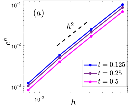
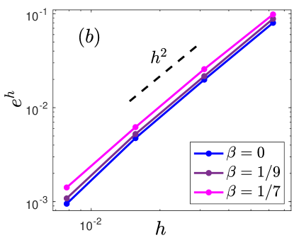
Fig. 1 presents the convergence rates of the proposed SP-PFEM (2.31) at different times and with different anisotropic strengths β\beta under a fixed time t=0.5t=0.5. It is apparent from this figure that the second-order convergence in space is independent of anisotropies and computation times, which indicates the convergence rate is very robust.

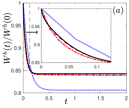
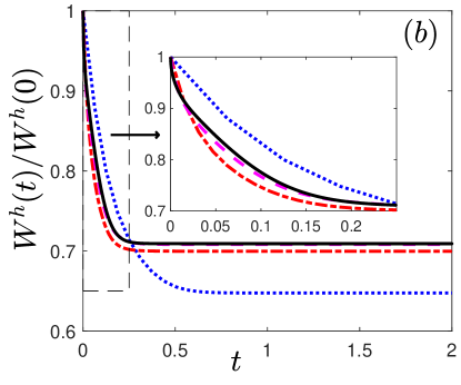
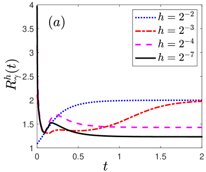
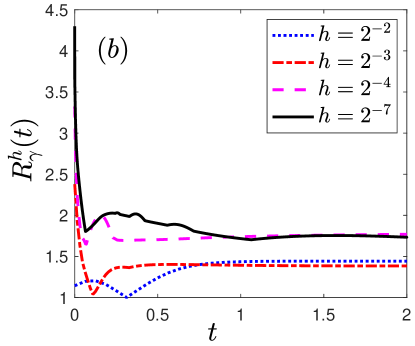
The time evolution of the normalized energy Wh(t)Wh(0)\frac{W^{h}(t)}{W^{h}(0)} with different hh, the normalized area loss ΔAh(t)Ah(0)\frac{\Delta A^{h}(t)}{A^{h}(0)} and the number of Newton iterations with h=27h=2^{-7}, and the weighted mesh quality Rγh(t)R^{h}_{\gamma}(t) with different hh are summarised in Figs. 2-4, respectively.

It can be seen from Figs. 2-4 that

(i) The normalized energy is monotonically decreasing when the surface energy satisfies the energy stable condition (2.37) (cf. Fig. 2);
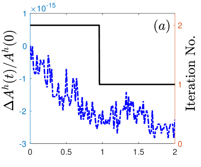
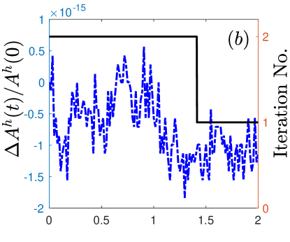
(ii) The normalized area loss is at 101510^{-15} which is almost at the same order as the round-off error (cf. Fig. 2), which confirms the area conservation in practical simulatoions;

(iii) Interestingly, the numbers of iterations in Newton’s method are initially 22 and finally 11 (cf. Fig. 3). This finding suggests that although the proposed SP-PFEM (2.31) is full-implicit, but it can be solved very efficiently with a few iterations;

(iv) In Fig. 4 there is a clear trend of convergence of the weighted mesh ratio RγhR_{\gamma}^{h}. Moreover, in contrast to the symmetrized SP-PFEM for symmetric γ(𝒏)\gamma(\boldsymbol{n}) in bao2021symmetrized , RγhR^{h}_{\gamma} keeps small even with the strongly anisotropy γ(𝒏)=1+13cos3θ\gamma(\boldsymbol{n})=1+\frac{1}{3}\cos 3\theta.

Refer to caption
Refer to caption
Refer to caption
Figure 2: Normalized energy of the SP-PFEM (2.31) with k(𝒏)=k0(𝒏)k(\boldsymbol{n})=k_{0}(\boldsymbol{n}) and different hh for: (a) anisotropy in Case I; (b) anisotropy in Case II with β=13\beta=\frac{1}{3}.
Refer to caption
Refer to caption
Figure 3: Normalized area loss (blue dashed line) and iteration number (black line) of the SP-PFEM (2.31) with k(𝒏)=k0(𝒏)k(\boldsymbol{n})=k_{0}(\boldsymbol{n}) and h=27,τ=h2h=2^{-7},\tau=h^{2} for: (a) anisotropy in Case I; (b) anisotropy in Case II with β=13\beta=\frac{1}{3}.
Refer to caption
Refer to caption
Figure 4: Weighted mesh ratio of the SP-PFEM (2.31) with k(𝒏)=k0(𝒏)k(\boldsymbol{n})=k_{0}(\boldsymbol{n}) and different hh for: (a) anisotropy in Case I; (b) anisotropy in Case II with β=13\beta=\frac{1}{3}.

5.2 Application for morphological evolutions

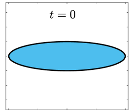
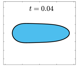
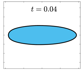
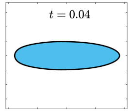
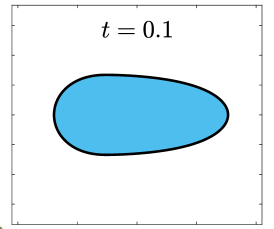
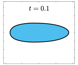
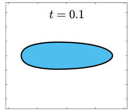
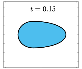
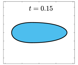
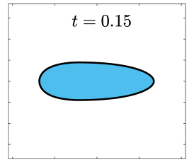
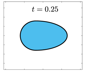
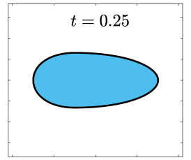
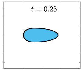
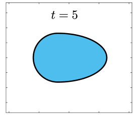
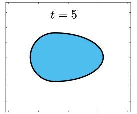
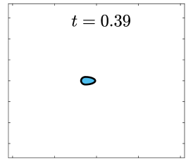
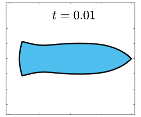
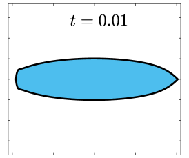
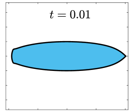
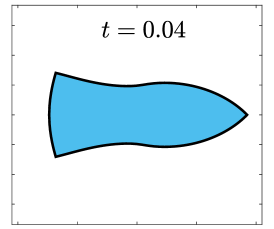
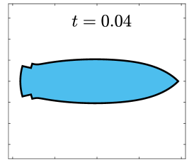
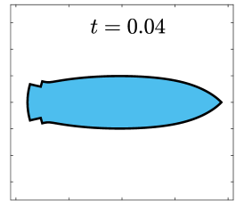
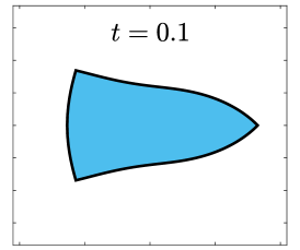
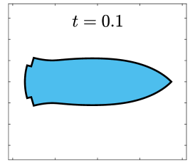
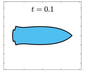
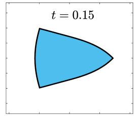
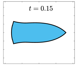
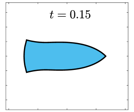
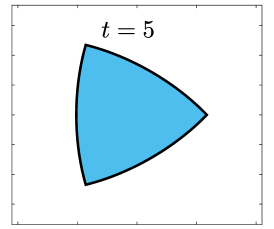
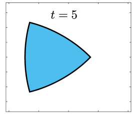
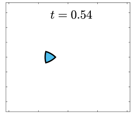
Finally, we apply the proposed SP-PFEMs to simulate the morphological evolutions driven by the three anisotropic geometric flows. Fig 5 plots the morphological evolutions of anisotropic surface diffusion for the four different anisotropic energies: (a) anisotropy in case I; (b)-(d) anisotropies in case II with β=1/9,1/7,1/3\beta=1/9,1/7,1/3, respectively. Fig 6 and Fig 7 depict the anisotropic surface diffusion, area-conserved anisotropic curvature flow, and anisotropic curvature flow at different times with anisotropy in case I and in case II with β=1/3\beta=1/3, respectively.

Refer to caption
Figure 5: Morphological evolutions of a 4×14\times 1 ellipse under anisotropic surface diffusion with four different anisotropic energies: (a) anisotropy in Case I; (b)-(d) anisotropies in case II with β=1/9,1/7,1/3\beta=1/9,1/7,1/3, respectively. The red and blue lines represent the initial curve and the numerical equilibrium, respectively; and the black dashed lines represent the intermediate curves. The mesh size and time step are taken as h=27,τ=h2h=2^{-7},\tau=h^{2}.

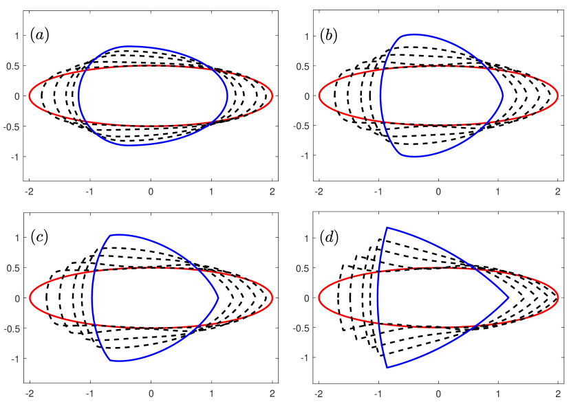
As shown in Fig. 5 (b)-(d), the edges emerge during the evolution and corners become sharper as the strength β\beta increases. In contrast, there are no edges or corners in the morphological evolutions with anisotropy in Case I. This suggests that even if it is not a C2C^{2}-function, it is more like weak anisotropy! From Fig. 6-7, we can see that the anisotropic surface diffusion and the area-conserved anisotropic curvature flow have the same equilibriums in shapes, while they have different dynamics, i.e., the equilibriums are different in positions, and the anisotropic surface diffusion evolves faster than the area-conserved anisotropic curvature flow.

Refer to caption
Refer to caption
Refer to caption
Refer to caption
Refer to caption
Refer to caption
Refer to caption
Refer to caption
Refer to caption
Refer to caption
Refer to caption
Refer to caption
Refer to caption
Refer to caption
Refer to caption
Refer to caption
Refer to caption
Refer to caption
Figure 6: Morphological evolutions of a 4×14\times 1 ellipse under anisotropic surface diffusion (left column), area-conserved anisotropic curvature flow (middle column) and anisotropic curvature flow (right column) with the anisotropic surface energy in Case I at different times. The evolving curves and their enclosed regions are colored by blue and black. The mesh size and time step are taken as h=27,τ=0.001h=2^{-7},\tau=0.001.
Refer to caption
Refer to caption
Refer to caption
Refer to caption
Refer to caption
Refer to caption
Refer to caption
Refer to caption
Refer to caption
Refer to caption
Refer to caption
Refer to caption
Refer to caption
Refer to caption
Refer to caption
Refer to caption
Refer to caption
Refer to caption
Figure 7: Morphological evolutions of a 4×14\times 1 ellipse under anisotropic surface diffusion (left column), area-conserved anisotropic curvature flow (middle column) and anisotropic curvature flow (right column) with the anisotropic surface energy in Case II with β=1/3\beta=1/3 at different times. The evolving curves and their enclosed regions are colored by blue and black. The mesh size and time step are taken as h=27,τ=0.001h=2^{-7},\tau=0.001.

6 Conclusions

By introducing a novel surface energy matrix 𝑮k(𝒏)\boldsymbol{G}_{k}(\boldsymbol{n}) depending on the anisotropic surface energy γ(𝒏)\gamma(\boldsymbol{n}) and the Cahn-Hoffman 𝝃\boldsymbol{\xi}-vector as well as a nonnegative stabilizing function k(𝒏)k(\boldsymbol{n}), we proposed conservative geometric partial differential equations for several geometric flows with anisotropic surface energy γ(𝒏)\gamma(\boldsymbol{n}). We derived their weak formulations and applied PFEM to get their full discretizations. Then we proved these PFEMs are structure-preserving under a very mild condition on γ(𝒏)\gamma(\boldsymbol{n}) with proper choice of the stabilizing function k(𝒏)k(\boldsymbol{n}). Though our surface energy matrix 𝑮k(𝒏)\boldsymbol{G}_{k}(\boldsymbol{n}) is no longer symmetric, our experiments had shown a robust second-order convergence rate in space and linear convergence rate in time and unconditional energy stability. Specifically, the mesh quality of the proposed SP-PFEM, i.e. the weighted mesh ratio is much smaller, is much better than that in the symmetrized SP-PFEM proposed recently for anisotropic surface diffusion with a symmetric surface energy bao2021symmetrized ; bao2022symmetrized . Moreover, our SP-PFEMs work well for the piecewise C2C^{2} anisotropy, which is a significant achievement compared with other PFEMs. In the future, we will generalize the surface energy matrix 𝑮k(𝒏)\boldsymbol{G}_{k}(\boldsymbol{n}) to three dimensions (3D) and propose efficient and accurate SP-PFEM for anisotropic geometric flows in 3D.

References

  • (1) B. Andrews, Volume-preserving anisotropic mean curvature flow, Indiana Univ. Math. J., (2001), pp. 783-827.
  • (2) W. Bao, H. Garcke, R. Nürnberg, and Q. Zhao, Volume-preserving parametric finite element methods for axisymmetric geometric evolution equations, J. Comput. Phys., 460 (2022), pp. 111180.
  • (3) W. Bao, W. Jiang, and Y. Li, A symmetrized parametric finite element method for anisotropic surface diffusion of closed curves, SIAM J. Numer. Anal., to appear (arXiv preprint arXiv:2112.00508), (2021).
  • (4) W. Bao, W. Jiang, Y. Wang, and Q. Zhao, A parametric finite element method for solid-state dewetting problems with anisotropic surface energies, J. Comput. Phys., 330 (2017), pp. 380-400.
  • (5) W. Bao and Y. Li, A symmetrized parametric finite element method for anisotropic surface diffusion in 3D, arXiv preprint arXiv:2206.01883, (2022).
  • (6) W. Bao and Q. Zhao, An energy-stable parametric finite element method for simulating solid-state dewetting problems in three dimensions, J. Comput. Math., to appear (arXiv preprint arXiv:2012.11404), (2020).
  • (7) W. Bao and Q. Zhao, A structure-preserving parametric finite element method for surface diffusion, SIAM J. Numer. Anal., 59 (2021), pp. 2775-2799.
  • (8) J. W. Barrett, H. Garcke, and R. Nürnberg, A parametric finite element method for fourth order geometric evolution equations, J. Comput. Phys., 222 (2007), pp. 441-467.
  • (9) J. W. Barrett, H. Garcke, and R. Nürnberg, Numerical approximation of anisotropic geometric evolution equations in the plane, IMA J. Numer. Anal., 28 (2008), pp. 292-330.
  • (10) J. W. Barrett, H. Garcke, and R. Nürnberg, On the parametric finite element approximation of evolving hypersurfaces in R3, J. Comput. Phys., 227 (2008),
  • (11) J. W. Barrett, H. Garcke, and R. Nürnberg, A variational formulation of anisotropic geometric evolution equations in higher dimensions, Numer. Math., 109 (2008), pp. 1-44.
  • (12) J. W. Barrett, H. Garcke, and R. Nürnberg, A variational formulation of anisotropic geometric evolution equations in higher dimensions, Eur. J. Appl. Math., 21 (2010), pp. 519-556.
  • (13) J. W. Barrett, H. Garcke, and R. Nürnberg, Parametric finite element approximations of curvature-driven interface evolutions, in Handb. Numer. Anal, 21 (2020), pp. 275-423.
  • (14) J. Cahn, Stability, microstructural evolution, grain growth, and coarsening in a two-dimensional two-phase microstructure, Acta Metall. Mater., 39 (1991), pp. 2189-2199.
  • (15) J. W. Cahn and J. E. Taylor Overview no. 113 surface motion by surface diffusion, Acta Metall. Mater., 42 (1994), pp. 1045-1063.
  • (16) W. C. Carter, A. Roosen, J. W. Cahn, and J. E. Taylor, Shape evolution by surface diffusion and surface attachment limited kinetics on completely faceted surfaces, Acta Metall. Mater., 43 (1995), pp. 4309-4323.
  • (17) Y. Chen, Y. Giga, and S. Goto, Uniqueness and existence of viscosity solutions of generalized mean curvature flow equations, in Fundamental Contributions to the Continuum Theory of Evolving Phase Interfaces in Solids, Springer, 1999, pp. 375-412.
  • (18) U. Clarenz, U. Diewald, and M. Rumpf, Anisotropic geometric diffusion in surface processing, IEEE Vis. 2000, 2000.
  • (19) K. Deckelnick, G. Dziuk, and C. M. Elliott, Computation of geometric partial differential equations and mean curvature flow, Acta Numer., 14 (2005), pp. 139-232.
  • (20) K. Deckelnick, G. Dziuk, and C. M. Elliott, Fully discrete finite element approximation for anisotropic surface diffusion of graphs, SIAM J. Numer. Anal., 43 (2005), pp. 1112-1138.
  • (21) I. C. Dolcetta, S. F. Vita, and R. March, Area-preserving curve-shortening flows: from phase separation to image processing, IFB, (2002), pp. 325-343.
  • (22) P. Du, M. Khenner, and H. Wong, A tangent-plane marker-particle method for the computation of three-dimensional solid surfaces evolving by surface diffusion on a substrate, J. Comput. Phys., 229 (2010), pp. 813-827.
  • (23) Q. Du and X. Feng, The phase field method for geometric moving interfaces and their numerical approximations, in Handb. Numer. Anal, 21 (2020), pp. 425-508.
  • (24) I. Fonseca, A. Pratelli and B. Zwicknagl, Shapes of epitaxially grown quantum dots, Arch. Ration. Mech. Anal., 214 (2014), pp. 359-401.
  • (25) P. M. Girao and R. V. Kohn, The crystalline algorithm for computing motion by curvature, in Variational Methods for Discontinuous Structures, Springer, 1996, pp. 7-18.
  • (26) M. E. Gurtin and M. E. Jabbour, Interface evolution in three dimensions with curvature-dependent energy and surface diffusion: interface-controlled evolution, phase transitions, epitaxial growth of elastic films, Arch. Ration. Mech. Anal., 163 (2002), pp. 171-208.
  • (27) D. W. Hoffman and J. W. Cahn, A vector thermodynamics for anisotropic surfaces: I. fundamentals and application to plane surface junctions, Surf. Sci., 31 (1972), pp. 368-388.
  • (28) W. Jiang, W. Bao, C. V. Thompson, and D. J. Srolovitz, Phase field approach for simulating solid-state dewetting problems, Acta Mater., 60 (2012), pp. 5578-5592.
  • (29) W. Jiang, Y. Wang, Q. Zhao, D. J. Srolovitz, and W. Bao, Solid-state dewetting and island morphologies in strongly anisotropic materials, Scr. Mater., 115 (2016), pp. 123-127.
  • (30) W. Jiang and Q. Zhao, Sharp-interface approach for simulating solid-state dewetting in two dimensions: A Cahn-Hoffman 𝝃\boldsymbol{\xi}-vector formulation, Phys. D, 390 (2019), pp. 69-83.
  • (31) B. Kovaács, B. Li, and C. Lubich, A convergent evolving finite element algorithm for mean curvature flow of closed surfaces, Numer. Math., 143 (2019), pp. 797-853.
  • (32) Y. Li and W. Bao, An energy-stable parametric finite element method for anisotropic surface diffusion, J. Comput. Phys., 446 (2021), p. 110658.
  • (33) W. J. Niessen, B. M. Romeny, L. M. Florack, and M. A. Viergever, A general framework for geometry-driven evolution equations, Int. J. Comput. Vis., 21 (1997), pp. 187-205.
  • (34) S. Randolph, J. Fowlkes, A. Melechko, K. Klein, H. Meyer, M. Simpson, and P. Rack, Controlling thin film structure for the dewetting of catalyst nanoparticle arrays for subsequent carbon nanofiber growth, Nanotech., 18 (2007), p. 465354.
  • (35) H. Shen, S. Nutt, and D. Hull, Direct observation and measurement of fiber architecture in short fiber-polymer composite foam through micro-CT imaging, Compos. Sci. Technol., 64 (2004), pp. 2113-2120.
  • (36) A. P. Sutton and R. W. Balluffi, Interfaces in crystalline materials, Clarendon Press, 1995.
  • (37) J. E. Taylor, Mean curvature and weighted mean curvature, Acta Metall. Mater., 40 (1992), pp. 1475-1485
  • (38) J. E. Taylor, J. W. Cahn, and C. A. Handwerker, Overview no. 98 i—geometric models of crystal growth, Acta Metall. Mater., 40 (1992), pp. 1443-1474.
  • (39) C. V. Thompson, Solid-state dewetting of thin films, Annu. Rev. Mater. Res., 42 (2012), pp. 399-434.
  • (40) Y. Wang, W. Jiang, W. Bao, and D. J. Srolovitz, Sharp interface model for solid-state dewetting problems with weakly anisotropic surface energies, Phys. Rev. B, 91 (2015), p. 045303.
  • (41) A. Wheeler, Cahn-Hoffman 𝝃\boldsymbol{\xi}-vector and its relation to diffuse interface models of phase transitions, J. Stat. Phys., 95 (1999), pp. 1245-1280.
  • (42) H. Wong, P. Voorhees, M. Miksis, and S. Davis, Periodic mass shedding of a retracting solid film step, Acta Mater., 48 (2000), pp. 1719-1728.
  • (43) Y. Xu and C. Shu, Local discontinuous Galerkin method for surface diffusion and Willmore flow of graphs, J. Sci. Comput., 40 (2009), pp. 375-390.
  • (44) J. Ye and C. V. Thompson, Mechanisms of complex morphological evolution during solid-state dewetting of single-crystal nickel thin films, Appl. Phys. Lett., 97 (2010), p. 071904.
  • (45) Q. Zhao, W. Jiang, and W. Bao, An energy-stable parametric finite element method for simulating solid-state dewetting, IMA J. Num. Anal., 41 (2021), pp. 2026-2055.