A Sparsity Adaptive Algorithm to Recover NB-IoT Signal from Legacy LTE Interference

As $\bm{H}_{\text{LTE}}$ defined after (1) is a circulant matrix, it can be diagonalized such that (5) can be rewritten as

where $\bm{\Lambda}_{\text{LTE}}$ is a diagonal matrix. After performing DFT over (7), we obtain the received signal in frequency domain:

Now, we are in a position to mitigate the LTE signal in (8). In light of $\bm{F}_{P}$ being an orthogonal matrix and $\bm{\Lambda}_{\text{LTE}}$ being a diagonal matrix, let $\bm{G}_{1}\triangleq\bm{F}_{P}^{H}\bm{\Lambda}_{\text{LTE}}^{-1}$, then, multiplying $\tilde{\bm{y}}$ by $\bm{G}_{1}$ gives

Next, by recalling the special structure of the ZP-OFDM system illustrated in Fig. 2, we can fully eliminate the LTE signal by using the zero-padding appended at the end of each OFDM block. To be specific, let $\bm{G}_{2}\triangleq\begin{bmatrix}\bm{0}_{v\times N}&\bm{I}_{v}\end{bmatrix}$, then, multiplying $\bm{y}_{1}$ by $\bm{G}_{2}$ yields

where $\bm{W}\triangleq\bm{G}_{2}\bm{G}_{1}\in\mathbb{C}^{v\times P}$ is known as an observation matrix. Thus, our remaining task is to recover the sparse signal $\tilde{\bm{y}}_{\text{NB}}$ from the postprocessed $\bm{y}_{2}$.

As shown in Fig. 3, when NB-IoT operates in the in-band mode, the NB-IoT signal in frequency domain occupies several consecutive subcarriers. More accurately, the number of subcarriers is allowed to be $1$, $3$, $6$ or $12$, i.e., $N_{\rm sc}\in\left\{1,3,6,12\right\}$. This feature implies that $\bm{y}_{2}$ shown in (10) is a linear combination of several consecutive column vectors of $\bm{W}$. In other words, the correlation coefficients of $\bm{y}_{2}$ and each column vector of $\bm{W}$ will show one or more spikes, which can be located by the $K$-means clustering.

Applying the least squares (LS) principle to (10), the optimization problem can be formulated as

where the objective function is indeed the $\ell_{2}$-norm of the residue error, that is, $r\triangleq\left\|\bm{y}_{2}-\bm{W}\tilde{\bm{y}}_{\text{NB}}\right\|_{2}$.

In principle, finding the support of $\tilde{\bm{y}}_{\text{NB}}$ amounts to choosing a set of consecutive column vectors of $\bm{W}$ such that their linear combination minimizes the residue error in (11). To this end, the correlation coefficient of $\bm{y}_{2}$ and each column of $\bm{W}$ is computed as

On account of the continuous distribution of the support of $\tilde{\bm{y}}_{\text{NB}}$ (cf. Fig. 3), we employ the $K$-means clustering algorithm to classify these coefficients by Euclidean distance [14]. Suppose that we obtain $Q$ clusters, say, $\left\{\mathcal{C}_{q}\right\}_{q=1}^{Q}$, where $\mathcal{C}_{q}$ contains correlation coefficients in the $q^{\rm th}$ cluster, then, the optimal cluster is determined by

where $\mathcal{C}_{\text{opt}}$ is the cluster with the largest mean value of the correlation coefficients. As a result, the optimal column index set is given by

Now, since $\bm{y}_{2}$ is more likely a linear combination of column vectors whose column indices belong to $\mathcal{S}_{\text{opt}}$, the optimization problem $\mathcal{P}1$ can be further simplified as

To deal with $\mathcal{P}2$, we define a count vector $\bm{f}_{P\times 1}$ initialized as a null vector, then, the SAMP algorithm is used to solve the minimization problem in (16) without considering the sparsity constraint in (17). With the estimated support denoted $\mathcal{I}$, the count vector $\bm{f}$ is updated as per

It is noteworthy that, in practice, the column vectors chosen by $\mathcal{S}_{\text{opt}}$ shown in (15) may be linearly dependent. If so, this dependence would degrade the recovery probability. To deal with this situation, we randomly disturb the columns of $\bm{W}$ to form a new observation matrix $\bm{W}^{\prime}$ and corresponding measurement vector $\bm{y}_{2}^{\prime}$. According to (13)-(15), a new optimal column index set $\mathcal{S}_{\text{opt}}^{\prime}$ is generated and $\bm{W}_{\mathcal{S}_{\text{opt}}}$ in $\mathcal{P}2$ is replaced by $\bm{W}_{\mathcal{S}_{\text{opt}}^{\prime}}$. Then, the SAMP algorithm is repeatedly used to solve the problem in (16) again. The estimated support is denoted $\mathcal{I}^{\prime}$, and the count vector $\bm{f}$ proceeds with updating by $\mathcal{I}^{\prime}$ according to (18). The aforementioned operations are repeated $R_{\max}$ times to obtain the final count vector $\bm{f}$, which is next used to refine the estimate of the support.

To minimize the $\ell_{2}$-norm of the residue error in (16), the estimated support $\mathcal{I}$ by the SAMP at each repetition described above does not satisfy the constraint in (17). Now, we exploit the final count vector $\bm{f}$ to refine the estimate of the support. It is not hard to understand that, after $R_{\max}$ repetitions, the final $\bm{f}$ contains the distribution information of the real support of NB-IoT signal. Since NB-IoT occupies several continuous subcarriers in the LTE spectrum, finding the real support of the NB-IoT signal is equivalent to finding an index range in $\bm{f}$ where an spike occurs.

The procedure to recover the support of NB-IoT signal from the final count vector $\bm{f}$ is as follows. First, we define a difference vector $\bm{d}\in\mathbb{R}^{P\times 1}$ with entries given by

Then, given the indices of the minimum and maximum values in the difference vector $\bm{d}$, denoted $p_{1}$ and $p_{2}$, respectively, determined by

the starting point and endpoint of the spike are located. Next, with $p_{1}$ and $p_{2}$, a sample set $\mathcal{X}$ can be generated as per

If ${\rm var}(\mathcal{X})<\epsilon$, then it implies that the elements of $\bm{f}$ between indices $p_{1}$ and $p_{2}$ shape one spike. Further, if $\text{Card}\left(\mathcal{X}\right)\in\left\{1,3,6,12\right\}$, the estimated optimal support is finally given by

Otherwise, repeat the aforementioned operations until ${\rm var}(\mathcal{X})<\epsilon$ and $\text{Card}\left(\mathcal{X}\right)\in\left\{1,3,6,12\right\}$. Simulation results to be discussed at the end of the next section demonstrate that the algorithm converges after $30$ repetitions.

With the optimal support estimated, the transmitted NB-IoT signal can be recovered by using the LS principle. Specifically, let $\bm{y}_{\text{LS}}\triangleq\bm{W}_{\mathcal{Z}^{*}}^{\dagger}\bm{y}_{2}$, then $\tilde{\bm{y}}_{\text{NB}}^{*}$ can be expressed as

To sum up, the developed algorithm to recover the NB-IoT signal from LTE interference is formalized in Algorithm 1.

Table I compares the computational complexity of the proposed algorithm with three benchmark ones developed in [7, 10, 11]. It is observed that the proposed algorithm has lower complexity than the classic SAMP [7], as the latter locates directly the support of NB-IoT subcarriers without any pre-estimate. The computational complexity of our algorithm and that in [11] (denoted ‘CWS’ for short) is independent of the number of NB-IoT subcarriers (i.e., $K$), whereas that in [10] (denoted ‘SCEM’ for short) increases quadratically with $K$. The proposed algorithm has a bit higher complexity than that in [11] because the latter assumes the prior sparsity of NB-IoT signal, which is however unknown in practice.

Figure 4 shows the recovery probability versus the number of NB-IoT subcarriers. In the pertaining simulation setup, the SNR is fixed to $23$ dB while the SIR is $20$ dB, which means that the system is interference dominated. It is seen from Fig. 4 that the recovery probability decreases with the number of NB-IoT subcarriers, as more subcarriers suffer higher interference. With sparsity known, the developed algorithm outperforms the SCEM and CWS algorithm and approaches the performance in the ideal case. On the other hand, in the case of unknown sparsity, the developed algorithm performs much better than the SCEM and SAMP algorithm.

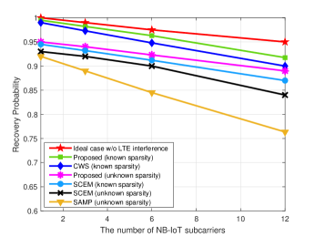
Figure 5 illustrates the bit error rate (BER) versus the SNR of the NB-IoT signal with known sparsity, where the SIR is fixed to $15$ dB and $N_{\rm sc}=6$ in the left panel (or $N_{\rm sc}=12$ in the right panel). It is seen that the BER decreases with SNR but increases with the number of NB-IoT subcarriers, as expected. In the case of $N_{\rm sc}=6$, given the target BER being $10^{-3}$, the left panel of Fig. 5 shows that the required SNR corresponding to the ideal case is about $12$ dB and the SNR required by the proposed algorithm is about $13$ dB, which outperforms the CWS algorithm by $3.5$ dB and the SCEM algorithm by $4$ dB.

Figure 6 depicts the BER versus the SNR of the NB-IoT signal with unknown sparsity, where the SIR is fixed to $20$ dB and $N_{\rm sc}=6$ in the left panel (or $N_{\rm sc}=12$ in the right panel). It shows that the BER of the proposed algorithm approaches that in the ideal case without interference whereas the SAMP and SCEM algorithm perform much worse.

Figure 7 shows the recovery probability versus the maximum repetition number $R_{\max}$ in each iteration. In the simulation setup, the number of NB-IoT subcarriers is set to $N_{\rm sc}=6$ with SNR being $23$ dB and SIR being $20$ dB. It is observed that all three curves converge after 30 repetitions. In the case of known sparsity, the proposed algorithm obtains $98\%$ recovery probability, which outperforms the CWS algorithm by $4\%$, albeit a bit slower convergence. In the case of unknown sparsity, the CWS algorithm does not work anymore but the proposed algorithm has a recovery probability about $90\%$.

References

- [1] Y. C. Eldar and G. Kutyniok, Compressed Sensing: Theory and Applications. Cambridge University Press, 2012.
- [2] A. Gomaa and N. Al-Dhahir, “A compressive sensing approach to NBI cancellation in mobile OFDM systems,” in Proc. IEEE GLOBECOM’2010, 2010, pp. 1–5.
- [3] H. Al-Tous, I. Barhumi, and N. Al-Dhahir, “Atomic-norm for joint data recovery and narrow-band interference mitigation in OFDM systems,” in Proc. IEEE PIMRC’2016, 2016, pp. 1–5.
- [4] H. Al-Tous, I. Barhumi, A. Kalbat, and N. Al-Dhahir, “ADMM for joint data and off-grid NBI recovery in OFDM systems,” in Proc. IEEE WCNC’2018, 2018, pp. 1–6.
- [5] X. Zhang, Y. Ma, Y. Gao, and S. Cui, “Real-time adaptively regularized compressive sensing in cognitive radio networks,” IEEE Trans. Veh. Technol., vol. 67, no. 2, pp. 1146–1157, Feb. 2018.
- [6] W. Dai and O. Milenkovic, “Subspace pursuit for compressive sensing signal reconstruction,” IEEE Trans. Inf. Theory, vol. 55, no. 5, pp. 2230–2249, May 2009.
- [7] T. T. Do, L. Gan, N. Nguyen, and T. D. Tran, “Sparsity adaptive matching pursuit algorithm for practical compressed sensing,” in Proc. 42nd ACSSC, 2008, pp. 581–587.
- [8] H. Xie, P. Wu, F. Tan, and M. Xia, “Adaptively-regularized compressive sensing with sparsity bound learning,” IEEE Commun. Lett., vol. 25, no. 4, pp. 1283–1287, Apr. 2021.
- [9] I. Daubechies, R. DeVore, M. Fornasier, and C. S. Güntürk, “Iteratively reweighted least squares minimization for sparse recovery,” Commun. Pure and Applied Math., vol. 63, no. 1, pp. 1–38, Jan. 2010.
- [10] S. Liu, L. Xiao, Z. Han, and Y. Tang, “Eliminating NB-IoT interference to LTE system: A sparse machine learning-based approach,” IEEE Internet of Things J., vol. 6, no. 4, pp. 6919–6932, Aug. 2019.
- [11] Y. Guo, P. Wu, and M. Xia, “Recovering NB-IoT signal from legacy LTE interference via K-means clustering,” in Proc. IEEE 93rd VTC’2021-Spring, Helsinki, Finland, Apr. 2021, pp. 1–5.
- [12] S. Liu, F. Yang, J. Song, and Z. Han, “Block sparse Bayesian learning-based NB-IoT interference elimination in LTE-advanced systems,” IEEE Trans. Commun., vol. 65, no. 10, pp. 4559–4571, Oct. 2017.
- [13] 3GPP, TS 36.211: “Evolved Universal Terrestrial Radio Access (E-UTRA); Physical Channels and Modulation (Release 15)”, 2018.
- [14] C. M. Bishop, Pattern Recognition and Machine Learning. Springer-Verlag New York, Inc., 2006, ch. 9, pp. 423–459.