A simplified Parisi Ansatz II:
Random Energy Model universality

Following ideas from Borgs, Chayes [12, 13], Coja-Oghlan [14] and others, in a recent paper we showed [4] that the scalar product of a spin state with some external field, that we call interface model, and formally describe with the Hamiltonian

$$H\left(\sigma_{V}|h_{V}\right):=\sigma_{V}\cdot h_{V},$$

(2)

can be approximated by the REM in the low temperature phase. The field components are real numbers $h_{i}\in\mathbb{R}$ indexed by $i\in V$ and are assumed to have been independently extracted from some probability distribution $p$. We use a braket notation for the average of the test function $f$ respect to the Gibbs measure $\xi$ (softmax)

$$\langle f\left(\sigma_{V}\right)\rangle_{\xi}:=\sum_{\sigma_{V}\in\Omega^{V}}f\left(\sigma_{V}\right)\,\exp\left[-\sigma_{V}\cdot\beta h_{V}+N\beta\zeta\left(\beta h_{V}\right)\right],$$

(3)

where $N$ is the number of spins and $\zeta$ is the free energy density per spin:

$$-\beta\zeta\left(\beta h_{V}\right):=\frac{1}{N}\sum_{i\in V}\log 2\cosh\left(\beta h_{i}\right).$$

(4)

We remark that the interface model is closely related to the “Number Partitioning Problem” (NPP) [11, 12, 13], and we may also refer to it as a random field model, or noise model. It correspond for example to the Random Field Ising Model (RIFM) in the limit of zero Ising interactions (or infinite field amplitude) and many other models. In general, the interface could be seen as the zero interaction limit of any lattice field theory of the kind described in [15].

In Section 3.1 we study the thermodynamic limit by quantile mechanics [16] and series analysis, and give explicit examples for the binary, uniform and Gaussian cases. The scaling limit of the free energy density for an infinite number of spins will converge almost surely to the following functional:

$$-\lim_{N\rightarrow\infty}\beta\zeta\left(\beta h_{V}\right)=\int_{0}^{1}dq\,\log 2\cosh\left[\beta x\left(q\right)\right].$$

(5)

The function $x\left(q\right)$ is called quantile and is found by inverting the cumulant of $p$,

$$q\left(x\right):=\int_{0}^{x}dz\ p\left(z\right),$$

(6)

by quantile mechanics [16] the quantile satisfies the differential equation

$$\partial_{q}^{2}x\left(q\right)=\rho\left[\,x\left(q\right)\right]\left[\partial_{q}\,x\left(q\right)\right]^{2},$$

(7)

where the function $\rho$ is defined from $p$ according to the relation

$$\rho\left(x\right):=-\partial_{x}\log p\left(x\right).$$

(8)

We explicitly compute the uniform and Gaussian cases. At high temperature we find that, as expected, the free energy is replica symmetric, and is therefore linear in temperature. At low temperature we find that the convergence toward the ground state energy is quadratic in the temperature, ie., the specific heat is linear like in the Dulong-Petit law. The origin of this quadratic convergence is due to vertices with small field amplitude (see Section 3), and notice that, if we restrict to linear terms, the low temperature modes can be neglected and the free energy is approximately constant in temperature, like in the REM. In Section 5 of [4] the convergence to the REM is actually shown in distribution in the near zero temperature phase.

To this scope we introduce the eigenstates of magnetization

$$\Omega\left(m\right):=\left\{\sigma_{V}\in\Omega^{V}:\,M(\sigma_{V})=\left\lfloor mN\right\rfloor\right\},$$

(9)

where $M(\sigma_{V})$ stands for the total magnetization of the state $\sigma_{V}$. These central objects of our analysis are studied in detail in Section 4. We also introduce the “master direction” $\omega_{V}$, the flickering state $\sigma_{V}^{*}$ and flickering function $f^{*}$

$$\omega_{i}:=h_{i}/|h_{i}|,\ \ \ \sigma_{i}^{*}:=\sigma_{i}\,\omega_{i},\ \ \ f^{*}\left(\sigma_{V}\right):=f\left(\sigma_{V}\circ\omega_{V}\right),$$

(10)

where $\omega_{i}$ is the direction of the ground state in the vertex $i$, and $f$ is any test function if not specified otherwise. We can now introduce a fundamental variable, that we call $J-$field: let define the following quantities

$$\psi:=\frac{1}{N}\sum_{i\in V}|h_{i}|,\ \ \ \delta^{2}:=\frac{1}{N}\sum_{i\in V}h_{i}^{2}-\psi^{2},\ \ \ J_{i}:=\frac{|h_{i}|-\psi}{\delta},$$

(11)

where $\psi$ denotes the ground state energy density and $\delta$ is the amplitude of the fluctuations of $|h_{i}|$ around $\psi$. As explained in the Sections 5 and 6, it is possible to track the fluctuations around the ground state. This is done by introducing the the vertex set $X$,

$$X\left(\sigma_{V}^{*}\right):=\left\{i\in V:\,\sigma_{i}^{*}=-1\right\},$$

(12)

that collects the vertices in which the spin $\sigma_{i}$ is flipped with respect to the direction of the ground state $\omega_{i}$, and the renormalized field $J$:

$$J(\sigma_{V}^{*}):=\frac{1}{\sqrt{|X(\sigma_{V}^{*})|}}\sum_{i\in X(\sigma_{V}^{*})}J_{i},$$

(13)

that is the normalized sum of the flipped local fields. The Hamiltonian of Eq. (2) can be expressed in terms of $M$, $J$ and $X$ as follows:

$$\sigma_{V}\cdot h_{V}=\psi M\left(\sigma_{V}^{*}\right)+J(\sigma_{V}^{*}){\textstyle\sqrt{4\delta^{2}|X(\sigma_{V}^{*})|}}.$$

(14)

In Section 5 we show that in the thermodynamic limit the average of Eq. (3) is mostly sampled from eigenstates of magnetization with eigenvalue

$$m_{0}\left(\beta\psi\right):=\tanh\left(\beta\psi\right).$$

(15)

For any $\sigma_{V}\in\Omega\left(m_{0}\right)$ we can rewrite the Hamiltonian as:

$$\sigma_{V}\cdot h_{V}=\psi\,m_{0}\left(\beta\psi\right)N+J(\sigma_{V}^{*}){\textstyle\sqrt{K\left[m_{0}\left(\beta\psi\right)\right]}}$$

(16)

where we introduced the auxiliary function

$$K(m):=2\delta^{2}(1-m)\,N.$$

(17)

In reference [4] we found that at low temperature the $J$ field applied to $\Omega\left(m_{0}\right)$ actually converges in distribution to a REM. This is done by noticing that when the temperature goes to zero the state align toward the direction of the ground state almost everywhere, and only a small fraction of spins is flipped in the opposite direction. Since the flipped spins are sparse two independent spin configurations will probabily have a small number of common flipped spins, that can be ignored, making the corresponding $J-$fields independent. In Section 6 we show that it is possible to extend the results of [4] to the full temperature range by properly renormalizing the $J$ field. In particular, we will introduce the $\Delta^{\prime}$ field, described in detail in the Section 6. It is shown that, when applied to the ensemble $\Omega(m_{0})$, this field is distributed like a REM by construction (i.e., a field where the pairwise overlap matrix is zero on average). In Section 6 we show that the $J$ is distributed like $\Delta^{\prime}$ up to a constant and a renormalization

$$J(\sigma_{V}){\textstyle\sqrt{K(m_{0})}}=\Delta^{\prime}(\sigma_{V}){\textstyle\sqrt{K^{\prime}(m_{0})}}+\mathrm{const.},\ \ \ K^{\prime}(m):=\delta^{2}(1-m^{2})\,N,$$

(18)

the renormalized amplitude is found in Section 6. By the averaging properties of PPP, a parameter $\lambda$ exists (dependent from $\beta$, $\psi$ and $\delta$) such that the Gibbs average satisfy the REM-PPP average formula [3, 4, 5, 6],

$$\lim_{N\rightarrow\infty}\langle f\left(\sigma_{V}\right)\rangle_{\xi}=\lim_{N\rightarrow\infty}\langle f^{*}\left(\sigma_{V}\right)^{\lambda}\rangle_{m_{0}}^{1/\lambda},$$

(19)

that in the subcritical region $\lambda\in\left[0,1\right]$ interpolates between the geometric and the arithmetic average. The importance of the REM universality to the spin glass physics is now evident in that one could directly apply this formula to Eq. (55) of [3] (or Eq. (6.20) of [4]) and find the full-RSB Parisi functional. This complets the steps to compute the free energy of the SK model (and many other models) with methods and concepts from [3, 4, 15], see Section 6 below and Section 5 of [4] for further details. Notice that, apart from disordered systems and lattice field theory, similar properties have been recently observed also in important neural network models. Of special interest is the relation with Dense Associative Memories (DAM): for example, in [17] has been shown that also in the exponential Hopfield models one can approximate the free energy of each layer with that of a REM.

Since the free energy depends only on the absolute value of the external field and not on the direction, before proceeding with the computations it is convenient to introduce the following auxiliary variables:

$$x_{i}=\left|h_{i}\right|,\ \ \ \omega_{i}=h_{i}/|h_{i}|,\ \ \ \sigma_{i}^{*}=\sigma_{i}\,\omega_{i}$$

(24)

the flickering state $\sigma_{V}^{*}$ is the Hadamard product between the initial state $\sigma_{V}$ and the direction of the external field $\omega_{V}$, that corresponds to the ground state of the system and that we call master direction. Using these variables the Hamiltonian can be rewritten as $\sigma_{V}^{*}\cdot x_{V}$ where $x_{V}$ is a vector with all positive entries, we call it rectified field. To find the scaling limit of the free energy it is convenient to reoreder $V$ according to the order statistics, a remapping of the index $i\in V$, usually denoted with the symbol $\left(i\right)$, such that $x_{\left(i\right)+1}\geq x_{\left(i\right)}$. Then, it is easy to see that if each $x_{i}$ is independently drawn according to the same probability density $p$, then the scaling limit of $x_{\left(i\right)}$ for $\left(i\right)/N\rightarrow q\in\left[0,1\right]$ will almost surely converge to the quantile function of $p$.

There are several important cases that can be treated exactly, one could consider the uniform distribution $p\left(x\right)=\mathbb{I}\left(x\in\left[0,1\right]\right)$: here the cumulant is $q\left(x\right)=x$ and the quantile is therefore $x\left(q\right)=q$, then, the free energy density converges to the following integral:

$$-\lim_{N\rightarrow\infty}\beta\zeta\left(\beta x_{V}\right)=\int_{0}^{1}dq\,\log 2\cosh\left(\beta q\right)=\frac{1}{\beta}\int_{0}^{\beta}d\tau\,\log 2\cosh\left(\tau\right)$$

(25)

the primitive of this integral is easily found via computer algebra,

$$\int d\tau\,\log 2\cosh\left(\tau\right)=\frac{\mathrm{Li_{2}\left[-\exp\left(-2\tau\right)\right]}+\tau^{2}}{2}$$

(26)

where $\mathrm{Li_{2}}$ is the dilogarithm [18], or Spence’s function, that is often encountered in particle physics: for $z\in\left[0,1\right]$ the following relations holds

$$\mathrm{Li_{2}}\left(-z\right)=\sum_{k\geq 1}\frac{\left(-z\right)^{k}}{k^{2}},\ \ \ \mathrm{Li_{2}\left(-1\right)}=-\frac{\pi^{2}}{12},\ \ \ \mathrm{Li_{2}}\left(0\right)=0,$$

(27)

the first derivative obeys the following formula

$$\partial_{z}\,\mathrm{Li_{2}}\left(-z\right)=\sum_{k\geq 1}\frac{\left(-z\right)^{k-1}\left(-1\right)}{k}=z^{-1}\sum_{k\geq 1}\frac{\left(-z\right)^{k}}{k}=\frac{\log\left(1-z\right)}{z}$$

(28)

and notice that at $-1$ the derivative converges to the nontrivial value

$$\partial_{z}\mathrm{Li_{2}}\left(-1\right)=-\log 2$$

(29)

Then, the scaling limit of the free energy density converges to the expression

$$-\lim_{N\rightarrow\infty}\beta\zeta\left(\beta x_{V}\right)=\frac{\beta}{2}+\frac{\pi^{2}}{24\,\beta}+\frac{\mathrm{Li_{2}\left[-\exp\left(-2\beta\right)\right]}}{2\beta},$$

(30)

where the last term is negative in the whole temperature range. Notice that the convergence to the ground state energy is quadratic in temperature: the specific heat is linear like in the Dulong-Petit law.

We could also consider more complex shapes, like the half-normal distribution,

$$p\left(x\right)=\sqrt{2/\pi}\ \exp\left(-x^{2}/2\right).$$

(31)

From quantile mechanics [16] one finds

$$\rho\left(x\right)=-\partial_{x}(-x^{2}/2+\log\sqrt{2/\pi}\,)=x,$$

(32)

then, the quantile equation and its boundary conditions is as follows:

$$\partial_{q}^{2}x\left(q\right)=x\left(q\right)\left[\partial_{q}\,x\left(q\right)\right]^{2},\ \ \ x\left(0\right)=0,\ \ \ x\left(1/2\right)=\sqrt{2\pi}\ \mathrm{erf^{-1}}\left(1/2\right),$$

(33)

solving the equation with these boundary give us

$$x\left(q\right)=\sqrt{2\pi}\ \mathrm{erf^{-1}}\left(q\right).$$

(34)

Then, for the half-normal (and normal) noise model we expect the free energy to converge toward the following limit expression

$$-\lim_{N\rightarrow\infty}\beta\zeta\left(\beta x_{V}\right)=\int_{0}^{1}dq\,\log 2\cosh\,[\,\beta\sqrt{2\pi}\ \mathrm{erf^{-1}}\left(q\right)].$$

(35)

We notice that the differential equation in Eq. (33) before is remarkably similar to the term in parentesis in Eq. (10) of [19], that is the nonlinear antiparabolic equation from which we obtain the Parisi functional. Further investigation on the relation between the Guerra interpolation theory and quantile mechanics would be certainly interesting, we hope to explore this in a future work.

To highligt the low temperature features it will be more instructive to rather perform a series analysis. We start from the expression

$$-\beta\zeta\left(\beta x_{V}\right)=\lim_{N\rightarrow\infty}\frac{1}{N}\sum_{i\in V}\log 2\cosh\left(\beta x_{i}\right),$$

(36)

the ground state in the thermodynamic limit (TL) is

$$-\zeta\left(\infty\right)=\lim_{N\rightarrow\infty}\lim_{\beta\rightarrow\infty}\frac{1}{N}\sum_{i\in V}x_{i}\tanh\left(\beta x_{i}\right)=\lim_{N\rightarrow\infty}\frac{1}{N}\sum_{i\in V}x_{i}=\sqrt{\frac{2}{\pi}},$$

(37)

where the numeric value is obtained by computing the average of $x$ with $x$ Gaussian variable of zero average and unitary variance:

$$\lim_{N\rightarrow\infty}\frac{1}{N}\sum_{i\in V}x_{i}=\sqrt{\frac{2}{\pi}}\int_{0}^{\infty}x\,\exp\left(-x^{2}/2\right)\,dx=\sqrt{\frac{2}{\pi}}\int_{0}^{\infty}\exp\left(-t\right)\,dt=\sqrt{\frac{2}{\pi}},$$

(38)

in the last step we applied the substitution $t=x^{2}/2$. Now, let consider the equivalent expression

$$\lim_{N\rightarrow\infty}\frac{1}{N}\sum_{i\in V}\log 2\cosh\left(\beta x_{i}\right)=\beta\sqrt{\frac{2}{\pi}}+\lim_{N\rightarrow\infty}\frac{1}{N}\sum_{i\in V}\log\left[1+\exp\left(-2\beta x_{i}\right)\right],$$

(39)

the logarithm can be expanded in the limit of large $\beta$,

$$\log\left[1+\exp\left(-2k\beta x_{i}\right)\right]=\sum_{k\geq 1}\frac{\left(-1\right)^{k-1}}{k}\exp\left(-2k\beta x_{i}\right),$$

(40)

the average of the exponential term can be computed by Gaussian integration

$$\lim_{N\rightarrow\infty}\frac{1}{N}\sum_{i\in V}\exp\,(-2k\beta x_{i})=\sqrt{\frac{2}{\pi}}\int_{0}^{\infty}dx\,\exp\,(-2k\beta x-x^{2}/2)=\\ =\exp\,(\,2k^{2}\beta^{2})\,\sqrt{\frac{2}{\pi}}\int_{0}^{\infty}dx\,\exp\,[-(\sqrt{2}k\beta+x/\sqrt{2}\,)^{2}]=\\ =\exp\,(\,2k^{2}\beta^{2})\,\sqrt{\frac{4}{\pi}}\int_{0}^{\infty}d(\sqrt{2}k\beta+x/\sqrt{2}\,)\,\exp\,[-(\sqrt{2}k\beta+x/\sqrt{2}\,)^{2}]=\\ =\exp\,(\,2k^{2}\beta^{2})\,\sqrt{\frac{4}{\pi}}\int_{\sqrt{2}k\beta}^{\infty}dt\,\exp\,(-t^{2})=\exp\,(\,2k^{2}\beta^{2})\ \mathrm{erfc}\,(\sqrt{2}k\beta),$$

(41)

the last substitution is $t=x/\sqrt{2}+\sqrt{2}k\beta$. We found a series representation for the free energy of the gaussian noise model

$$-\beta\zeta\left(\beta x_{V}\right)=\beta\sqrt{\frac{2}{\pi}}+\sum_{k\geq 1}\frac{\left(-1\right)^{k-1}}{k}\exp\,(2k^{2}\beta^{2})\,\mathrm{erfc}(\sqrt{2}k\beta).$$

(42)

For large $\beta$ one can use the following approximation for the Error Function

$$\exp\,(2k^{2}\beta^{2})\,\mathrm{erfc}(\sqrt{2}k\beta)=\frac{1}{\sqrt{2\pi}k\beta}+O\left(\beta^{-3}\right).$$

(43)

Put the last expression back into the logarithm expansion before and one finds:

$$\lim_{N\rightarrow\infty}\frac{1}{N}\sum_{i\in V}\log\left[1+\exp\left(-2\beta x_{i}\right)\right]=\frac{K_{0}}{\sqrt{2\pi}\beta}+O\left(\beta^{-3}\right),$$

(44)

where the constant $K_{0}$ is the convergent sum

$$K_{0}:=\sum_{k\geq 1}\frac{\left(-1\right)^{k-1}}{k^{2}}=\frac{\pi^{2}}{12}$$

(45)

The asymptotic expansion of $\zeta$ near zero temperature is then found to be

$$-\beta\zeta\left(\beta x_{V}\right)=\beta\sqrt{\frac{2}{\pi}}+\frac{1}{\beta}\sqrt{\frac{\ \pi^{3}}{48}}+O\left(\beta^{-3}\right),$$

(46)

also in this case the convergence to the ground state is quadratic in temperature.

The origin of the quadratic difference in the low temperature behavior is in that for both uniform and Gaussian distributions some couplings may be close to zero for a fraction of spins. To see this, let analyze the energy contribution from the subset of spins

$$V\left(\delta\right)=\left\{i\in V:\>x_{i}>\delta\right\},$$

(47)

following the steps before we find

$$\int_{\delta}^{\infty}dx\,\exp\,(-2k\beta x-x^{2}/2)=\\ =\exp\,(2k^{2}\beta^{2})\,\mathrm{erfc}(\delta/\sqrt{2}+\sqrt{2}k\beta)=O\left[\exp\,(-2\delta k\beta)\right].$$

(48)

and then the limit in Eq. (44) restricted to $V\left(\delta\right)$ is

$$\lim_{N\rightarrow\infty}\ \frac{1}{|V\left(\delta\right)|}\sum_{i\in V\left(\delta\right)}\log\left[1+\exp\left(-2\beta x_{i}\right)\right]=O\left[\exp\,(-2\delta\beta)\right],$$

(49)

we can see if we exclude the spins with small coupling the temperature dependence is again exponentially suppressed in $\beta$.

Notice that the set $\Omega\left(M\right)$ is equivalent to a self-avoiding lattice gas of $E=N/2-M/2$ particles on a lattice of size $N$. Let define the particle displacements

$$X\left(\sigma_{V}\right):=\left\{i\in V:\,\sigma_{i}=-1\right\}\subset V$$

(54)

in the magnetic representation would be the subsets of $V$ where the flickering state $\sigma_{V}^{*}$ is flipped with respect to the master direction $1_{V}$ (that indicates a vector with all $1$ entries). Inside $\Omega\left(M\right)$ the size of $X$ is fixed, and related to the magnetization by

$$|X\left(\sigma_{V}\right)|=\left(N-M\right)/2=:E,\ \ \forall\sigma_{V}\in\Omega\left(M\right).$$

(55)

We interpret $E$ as the number of particles in our self-avoiding gas. Then, we introduce the set of all possible displacements of $E=\left\lfloor\epsilon N\right\rfloor$ particles

$$\mathcal{V}\left(E\right):=\left\{X\subset V:\,|X|=E\right\},$$

(56)

as for the magnetic rapresentation before we use the notation

$$\mathcal{V}\left(\left\lfloor\epsilon N\right\rfloor\right)=:\mathcal{V}\left(\epsilon\right),\ \ \ \langle f\left(\sigma_{V}\right)\rangle_{\mathcal{V}\left(\left\lfloor\epsilon N\right\rfloor\right)}=:\langle f\left(\sigma_{V}\right)\rangle_{\epsilon}.$$

(57)

that is in fact the exact image of $\Omega\left(m\right)$ if one takes $\epsilon=\left(1-m\right)/2$. We represent the spin states in terms of $X$ as follows: let $\sigma_{V}=\sigma_{V\setminus X}\cup\sigma_{X}$, then for the flipped spins we have $\sigma_{X}=-1_{X}$, vector with all negative entries, for the others $\sigma_{V\setminus X}=1_{V\setminus X}$ with all positive entries. The spin state $\sigma_{V}$ can be reconstructed from the flipped vertices

$$\sigma_{V}=1_{V\setminus X}\cup(-1_{X}),$$

(58)

this representation in terms of particle displacements allows to easily explore the overlap structure. Consider two configurations $X,Y\in\mathcal{V}\left(\epsilon\right)$, corresponding to

$$\sigma_{V}=1_{V\setminus X}\cup(-1_{X}),\ \ \tau_{V}=1_{V\setminus Y}\cup(-1_{Y}).$$

(59)

Within $\mathcal{V}\left(\epsilon\right)$ the number of particles is fixed $\left|X\right|=\left|Y\right|=\epsilon N$. Now, let $X\cap Y$ be the set of points of $V$ at which the two particle configurations $X$ and $Y$ overlap, and define the non-overlapping components

$$X^{\prime}:=X\setminus\left(X\cap Y\right),\ \ Y^{\prime}:=Y\setminus\left(X\cap Y\right),$$

(60)

that correspond to the non overlapping points of the particle displacements. By definition, their intersection is void, ie $X^{\prime}\cap Y^{\prime}=\textrm{ }$, moreover, the following equalities hold for of the union of $X$ and $Y$

$$X\cup Y=X^{\prime}\cup Y^{\prime}\cup\left(X\cap Y\right),\ \ X^{\prime}\cup Y^{\prime}=\left(X\cup Y\right)\setminus\left(X\cap Y\right).$$

(61)

It follows that $|X\cup Y|$ total fraction of $V$ occupied by the particles is

$$\left|X\cup Y\right|=\left|X\right|+\left|Y\right|-\left|X\cap Y\right|,$$

(62)

while the total non-overlapping volume is

$$\left|X^{\prime}\cup Y^{\prime}\right|=\left|X\cup Y\right|-\left|X\cap Y\right|=\left|X\right|+\left|Y\right|-2\left|X\cap Y\right|.$$

(63)

The overlap between the corresponding spin states can be expressed as

$$\sigma_{V}\cdot\tau_{V}=\left[1_{V\setminus X}\cup(-1_{X})\right]\cdot\left[1_{V\setminus Y}\cup(-1_{Y})\right]=\\ =N-2|X^{\prime}|-2|Y^{\prime}|=N-2\left|X\right|-2\left|Y\right|+4\left|X\cap Y\right|,$$

(64)

since we are considering magnetizations eigenstates with fixed eigenvalue, the volumes of $\left|X\right|$ and $\left|Y\right|$ are also fixed at $\epsilon N$, and the overlap of the spin states can be expressed in terms of the overlap between the particle configurations:

$$\sigma_{V}\cdot\tau_{V}=\left(1-4\epsilon\right)N+4\left|X\cap Y\right|.$$

(65)

The overlap size is $0\leq\left|X\cap Y\right|\leq\epsilon N$, but it can be shown (e.g., see the next section) that for large $N$ the overlap concentrates on $\epsilon^{2}N$, with fluctuations of order $\sqrt{N}$ (it converges to a gaussian), then from $m=1-2\epsilon$ and the Eq. (64) follows that the spin overlap concentrates almost surely on the mean value $1-4\epsilon+4\epsilon^{2}=m^{2}$.

We compute the probability that two configuration randomly extracted from $\mathcal{V}\left(\epsilon\right)$ have an intersection of size $\left\lfloor xN\right\rfloor$, with $x\in\left[0,\epsilon\right]$. The limit entropy density (rate function) of such event is defined as follows

$$\eta\left(x|\epsilon\right):=-\lim_{N\rightarrow\infty}\frac{1}{N}\log P\left(\,\left|X\cap Y\right|=\left\lfloor xN\right\rfloor\,|\,X,Y\in\mathcal{V}\left(\epsilon\right)\right)$$

(66)

that gives the shape of the distribution for large number of spins

$$P\left(\,\left|X\cap Y\right|=\left\lfloor xN\right\rfloor\,|\,X,Y\in\mathcal{V}\left(\epsilon\right)\right)\sim\exp\left[-N\eta\left(x|\epsilon\right)\right].$$

(67)

The first step is to notice that due to the uniformity of the distribution of the flipped spins the intersection size does not depend on the special realization of both states, then we can fix one of the two states: let’s fix $Y$ and call it ‘target’ set, then

$$P\left(\,\left|X\cap Y\right|=\left\lfloor xN\right\rfloor\,|\,X,Y\in\mathcal{V}\left(\epsilon\right)\right)=\\ =P\left(\,\left|X\cap Y\right|=\left\lfloor xN\right\rfloor\,|\,X\in\mathcal{V}\left(\epsilon\right)\right),\ \forall Y\in\mathcal{V}\left(\epsilon\right).$$

(68)

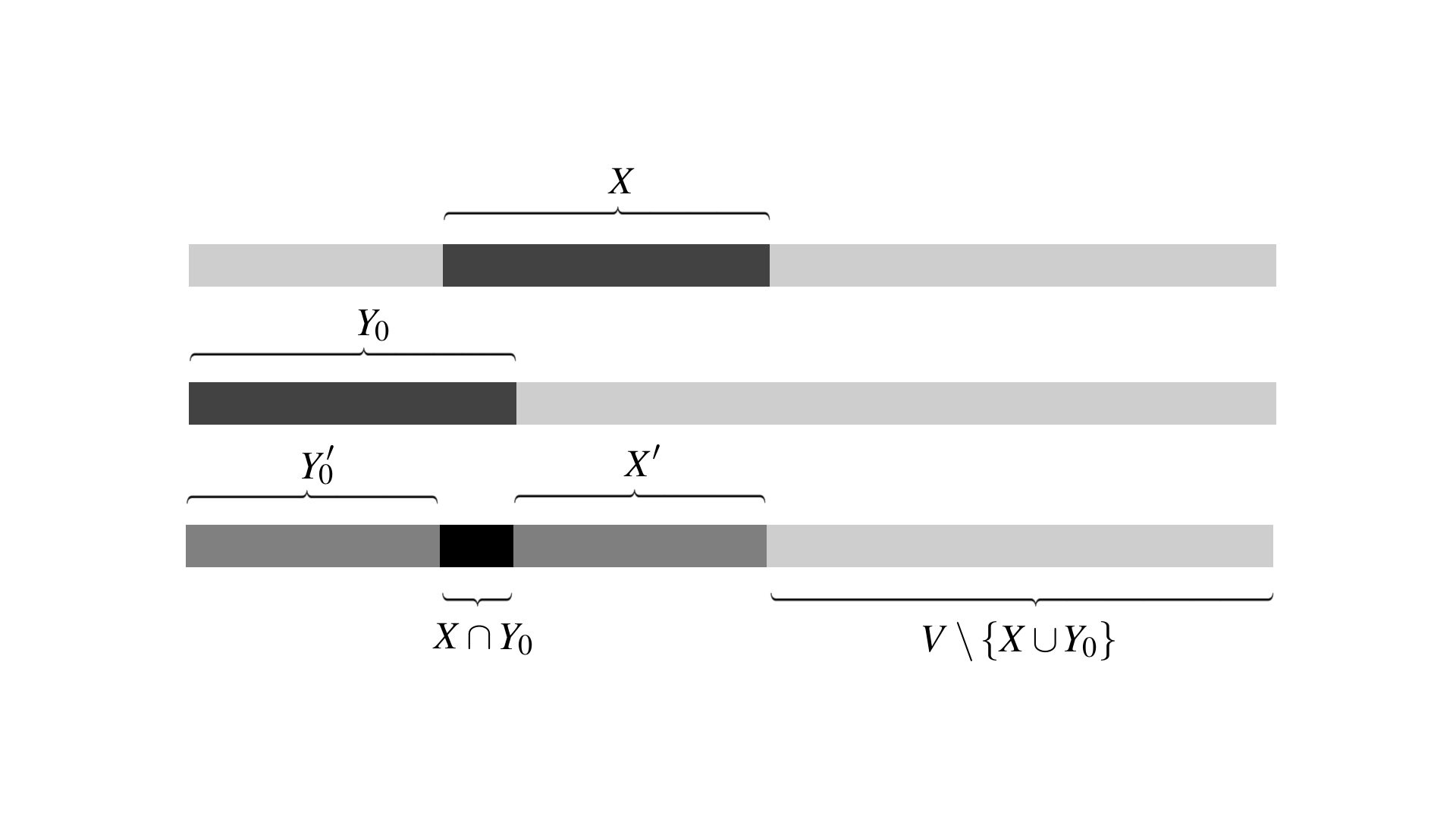
Since only the size of the target set actually matters, to highligth its internal components it will be convenient to chose a special configuration of the target (see Figure 1)

$$Y_{0}:=\left\{1\leq k\leq\left\lfloor\epsilon N\right\rfloor\right\}$$

(69)

where the vertices of the flipped spins are placed at the beginning of the set $V$ (ie, the labels $k\in V\setminus Y_{0}$ are all larger than $\left\lfloor\epsilon N\right\rfloor$), formally holds that

$$P\left(\,\left|X\cap Y\right|=\left\lfloor xN\right\rfloor\,|\,X,Y\in\mathcal{V}\left(\epsilon\right)\right)=P\left(\,\left|X\cap Y_{0}\right|=\left\lfloor xN\right\rfloor\,|\,X\in\mathcal{V}\left(\epsilon\right)\right),$$

(70)

The entropy density is given by the limit

$$\eta\left(x|\epsilon\right):=-\lim_{N\rightarrow\infty}\frac{1}{N}\log P\left(\,\left|X\cap Y_{0}\right|=\left\lfloor xN\right\rfloor\,|\,X\in\mathcal{V}\left(\epsilon\right)\right),$$

(71)

and it can be computed in many ways by Varadhan Lemma, the Mogulskii theorem and other large deviations techniques.

We can adapt methods from the urn process theory (see [22, 23]) to compute the shape of the overlap entropy density. The method consists in defining a nested set sequence that start from the null set and converges to $X$ in exactly $E$ steps,

$$X_{n}:=\bigcup_{n\leq E}\left\{i_{n}\right\},$$

(72)

that is a markov chain with transition matrix

$$P\left(i_{n+1}=k\right)=\frac{\mathbb{I}\left(\,k\in V\setminus X_{n}\right)}{\left|V\setminus X_{n}\right|}.$$

(73)

We indicate the overlap between $X_{n}$ and the target set $Y_{0}$ with

$$R_{n}:=\left|X_{n}\cap Y_{0}\right|,$$

(74)

the final conditions of the processes are fixed at $X_{E}=X$ and $R_{E}=\left|X\cap Y_{0}\right|$ respectively, reached in $E=\left\lfloor\epsilon N\right\rfloor$ steps. It can be shown that the overlap between $X_{n}$ and the target set follows a urn process [21, 22, 23, 24, 25] in the step variable $n$

$$R_{n+1}=\left\{\begin{array}[]{ccc}R_{n}+1&&\pi_{n}\left(R_{n}\right)\\ R_{n}&&1-\pi_{n}\left(R_{n}\right)\end{array}\right.$$

(75)

the urn function $\pi_{n}$ at step $n$ is the ratio between the number of vertices in $Y_{0}$ that have not been occupied in the preceeding $n$ extractions (that are $E-R_{n}$) and the number of vertices of $V$ that have not been occupied (ie, $N-n$),

$$\pi_{n}\left(R_{n}\right):=\frac{E-R_{n}}{N-n}.$$

(76)

adapting large-deviation methods [21, 22, 23, 24, 25] from generalized urn models is possible to show that the distribution of the overlap is aproximately Gaussian. It is also possible to compute the parameters by solving the difference equation

$$\mathbb{E}\left(R_{n+1}\right)=\mathbb{E}\left[\left(R_{n}+1\right)\pi_{n}\left(R_{n}\right)\right]+\mathbb{E}\left\{R_{n}\left[1-\pi_{n}\left(R_{n}\right)\right]\right\}$$

(77)

where $\mathbb{E}\left(\,\cdot\,\right)$ indicates the average respect to the urn process. Substituting the expression of the urn function we find

$$\mathbb{E}\left(R_{n+1}\right)-\mathbb{E}\left(R_{n}\right)=-\frac{1}{N-n}\mathbb{E}\left(R_{n}\right)+\frac{E}{N-n},$$

(78)

solving with null initial condition brings to the linear average solution $\mathbb{E}\left(R_{n}\right)=nE/N$ from which follows that the average overlap converges to

$$\lim_{N\rightarrow\infty}\frac{\langle\left|X\cap Y_{0}\right|\rangle_{\epsilon}}{N}=\lim_{N\rightarrow\infty}\frac{\mathbb{E}\left(R_{E}\right)}{N}=\epsilon^{2}.$$

(79)

We can show that the fluctuations are small: consider

$$\mathbb{E}\left(R_{n+1}^{2}\right)=\mathbb{E}[\left(R_{n}+1\right)^{2}\pi_{n}\left(R_{n}\right)]+\mathbb{E}\left\{R_{n}^{2}\left[1-\pi_{n}\left(R_{n}\right)\right]\right\},$$

(80)

substituting the urn function and the formula for the linear we find

$$\mathbb{E}\left(R_{n+1}^{2}\right)-\mathbb{E}\left(R_{n}^{2}\right)=-\frac{2}{N-n}\,\mathbb{E}\left(R_{n}^{2}\right)+\frac{E}{N-n}\left[1+n\left(\frac{2E-1}{N}\right)\right],$$

(81)

solving again for null initial condition gives another linear solution

$$\mathbb{E}\left(R_{n}^{2}\right)=\frac{nE\left[E\left(n-1\right)-n+N\right]}{N\left(N-1\right)}$$

(82)

Let now compute the variance of $R_{n}$: the variance is defined by

$$\mathbb{E}\left(R_{n}^{2}\right)-\mathbb{E}\left(R_{n}\right)^{2}=\frac{nE\left[E\left(n-1\right)-n+N\right]}{N\left(N-1\right)}-\frac{n^{2}E^{2}}{N^{2}}$$

(83)

and after some algebra it can be shown that for the variance holds

$$\lim_{N\rightarrow\infty}\frac{\langle\left|X\cap Y_{0}\right|^{2}\rangle_{\epsilon}-\langle\left|X\cap Y_{0}\right|\rangle_{\epsilon}^{2}}{N}=\lim_{N\rightarrow\infty}\frac{\mathbb{E}\left(R_{E}^{2}\right)-\mathbb{E}\left(R_{E}\right)^{2}}{N}=\epsilon^{2}\left(1-\epsilon\right)^{2}.$$

(84)

The entropy density $\eta$ can thus be expanded at second order in the variable

$$\Lambda\left(x|\epsilon\right):=\frac{x-\epsilon^{2}}{\epsilon\left(1-\epsilon\right)},$$

(85)

in the limit of large $N$ it can be shown that

$$\eta\left(x|\epsilon\right)=\frac{1}{2}\,\Lambda\left(x|\epsilon\right)^{2}+O[\,\Lambda\left(x|\epsilon\right)^{3}],$$

(86)

and since $m=1-2\epsilon$, according to Eq. (64), the corresponding spin overlap concentrates almost surely on the average value, ie., $1-4\epsilon+4\epsilon^{2}=m^{2}$. Notice that the spin overlap concentrates on the same value of the correlation matrix $\langle\sigma_{i}\sigma_{j}\rangle_{m}=m^{2}$. This means that the kernel of the magnetization eigenstates commutes in distribution, ie., that the correlation matrix converges to the overlap matrix, see in Section 2 of [4] for further details on kernel commutation and its implications.

In the low temperature limit the free energy is

$$-\beta\zeta\left(\beta\right)=\beta+\exp\left(-2\beta\right)+O\left[\exp\,(-4\beta)\right],$$

(90)

then, the free energy per spin converges to the ground state energy $\zeta\left(\infty\right)$ exponentially fast in $\beta$. Moreover, we find at high temperature the free energy converges to the replica symmetric (RS) free energy of the spin glass theory: Taylor expansion of the $\log\cosh$ function for small $\beta$ gives

$$-\beta\zeta\left(\beta\right)=\log 2+\frac{\beta^{2}}{2}+O\left(\beta^{4}\right).$$

(91)

It can be shown that in the zero temperature limit the Gibbs measure can be approximated by a random energy model: this will be discussed later.

References

- [1] Spin Glass Theory and beyond: An Introduction to the Replica Method and Its Applications, Parisi, G., Mezard, M., Virasoro, M., World Scientific, 1-476 (1986).
- [2] Spin Glass Theory and Far Beyond: Replica Symmetry Breaking After 40 Years, Charbonneau, P., Marinari, E., Mezard, M., Parisi, G., Ricci-Tersenghi, F., Sicuro, G., Zamponi, F. (eds), World Scientific, 1-740 (2023).
- [3] A simplified Parisi Ansatz, Franchini, S., Commun. Theor. Phys., 73, 055601 (2021).
- [4] Replica Symmetry Breaking without replicas, Franchini, S., Annals of Physics, 450, 169220 (2023).
- [5] Mean-field Spin Glass models from the Cavity-ROSt perspective, Aizenmann, M., Sims, R., Starr, S., AMS Contemporary Mathematics Series, 437, 1-30 (2007).
- [6] Derrida’s generalised random energy models 1: models with finitely many hierarchies, Bovier, A., Kurkova, I., Annales de l’I.H.P. Probabilit s et statistiques, 40 (4), 439-480 (2004).
- [7] REM Universality for Random Hamiltonians. Arous, G. B., Kuptsov, A., In: Spin Glasses: Statics and Dynamics, de Monvel, A., Bovier, A. (eds), Progress in Probability, 62, 45–84 (2009).
- [8] On constructing folding heteropolymers, Ebeling, M., Nadler, W., PNAS, 92 (19), 8798-8802 (1995).
- [9] Random costs in combinatorial optimization, Mertens, S., Phys. Rev. Lett. 84 (6), 1347–1350 (2000).
- [10] Phase transition and finite-size scaling for the integer partitioning problem. Borgs, C., Chayes, J., Pittel, B., Random Struct. Algorithms, 19 (3–4), 247–288 (2001). Analysis of algorithms, Krynica Morska, (2000).
- [11] Number partitioning as a random energy model, Bauke, H., Franz, S., Mertens, S., J. Stat. Mech. Theory Exp., 2004, P04003 (2004).
- [12] Proof of the local REM conjecture for number partitioning. I. Constant energy scales. Borgs, C., Chayes, J., Mertens, S., Nair, C., Random Struct. Algorithms, 34 (2), 217–240 (2009).
- [13] Proof of the local REM conjecture for number partitioning. II. Growing energy scales. Borgs, C., Chayes, J., Mertens, S., Nair, C., Random Struct. Algorithms, 34 (2), 241–284 (2009).
- [14] Harnessing the Bethe Free Energy, Bapst, V., Coja-Oghlan, A., Random Struct. Algorithms, 49, 694-741 (2016).
- [15] Neural activity in quarks language: Lattice Field Theory for a natwork of real neurons, Bardella, G., Franchini, S., Pan, L., Balzan, R., Ramawat, S., Brunamonti, E., Pani, P., Ferraina, S., Entropy, 26 (6), 495 (2024).
- [16] Quantile mechanics, Steinbrecher, G., Shaw, W. T., Eur. J. Appl. Math., 19 (2), 87-112 (2008).
- [17] The Exponential Capacity of Dense Associative Memories, Lucibello, C., Mezard M., Phys. Rev. Lett., 132, 077301 (2024).
- [18] The Dilogarithm Function, Zagier, D., In: Frontiers in Number Theory, Physics, and Geometry. II, Cartier, P., Moussa, P., Julia, B., Vanhove, P. (eds), Springer, Berlin, Heidelberg (2007).
- [19] Broken Replica Symmetry Bounds in the Mean Field Spin Glass Model, Guerra, F., Comm. Math. Phys., 233 (1), 1-12 (2003).
- [20] Large Deviations Techniques and Applications, Dembo, A., Zeitouni, O., Springer Berlin, 1-399 (1998).
- [21] Large deviations for generalized Polya urns with general urn functions, Franchini, S., PhD thesis, Universit Roma 3 (2015). http://hdl.handle.net/2307/5212
- [22] Large deviations for generalized Polya urns with arbitrary urn function, Franchini, S., Stoch. Proc. Appl., 127 (10), 3372-3411 (2017).
- [23] Large-deviation theory of increasing returns, Franchini, S., Balzan, R., Phys. Rev. E, 107, 064142 (2023).
- [24] Random polymers and generalized urn processes, Franchini, S., Balzan, R., Phys. Rev. E, 98, 042502 (2018).
- [25] Large deviations in models of growing clusters with symmetry-breaking transitions, Jack, R. L., Phys. Rev. E, 100, 012140 (2019).
- [26] Contributions to Random Energy Models, Jana, N. K. arXiv:0711.1249 (2007).