A Simple Model of Dark Matter and CP Violation
Abstract
We propose a simple model of dark matter and CP violation and consider the associated triple and quadruple productions of 125 GeV Higgs bosons at the Large Hadron Collider (LHC). In the model, the dark matter is a vector-like dark fermion interacting with the Standard Model only through a complex messenger scalar which is an electroweak singlet. New sources of CP violation reside in the most general scalar potential involving the doublet and the singlet , as well as in the dark Yukawa coupling between and . We study current experimental constraints from Higgs measurements, searches for new scalars at the LHC, precision electroweak measurements, EDM measurements, dark matter relic density, as well as direct and indirect detections of dark matter. A smoking-gun signature of CP violation could come from the Higgs-to-Higgs decays, , where are the heaviest scalar, second heaviest scalar and the SM-like 125-GeV Higgs, respectively. Taking into account other Higgs-to-Higgs decays, such as and , then gives rise to novel and final states, which have yet to be searched for experimentally. We present four benchmarks and show the event rates for and final states could be as large as and , respectively, at the 14-TeV LHC. This work opens up a new frontier of searching for triple and quadruple Higgs bosons at a high energy collider.
I Introduction
Dark matter and CP violation (CPV) are two of the most pressing puzzles in physics nowadays. Both relate to our own being in the Universe: dark matter is necessary for structure formation and CPV is a required condition for the observed matter-antimatter asymmetry. In particular, there is no cold dark matter candidate in the Standard Model (SM) of particle physics and the amount of CPV in the SM is insufficient to generate the observed baryon asymmetry. Consequently, both problems hint at the presence of new physics beyond the SM.
In this work we propose a simple extension of the SM to accommodate the dark matter and new sources of CPV, by including a vector-like dark fermion as the dark matter and a complex singlet scalar as the messenger mediating interactions between the SM and the dark matter. The most general scalar potential involving the Higgs doublet and the singlet contains several new sources of CPV, as does the dark Yukawa coupling between and . The complex singlet scalar extended SM has been studied in many contexts, such as the CPV, electroweak baryogenesis (EWBG), electroweak phase transition (EWPT), and scalar dark matter Barger et al. (2009); Chiang and Senaha (2008); Alexander-Nunneley and Pilaftsis (2010); Barger et al. (2010); Gonderinger et al. (2012); Gabrielli et al. (2014); Jiang et al. (2016); Darvishi and Krawczyk (2021); Darvishi and Masouminia (2017); Chiang et al. (2018); Chiang and Lu (2020); Robens et al. (2020). Our model is distinct in that i) we do not impose any discrete symmetries in the scalar potential, ii) the dark matter candidate is a vector-like dark fermion, instead of a component of the singlet scalar, and iii) new sources of CPV are confined in the scalar potential and the dark Yukawa coupling.111If the complex singlet scalar only couples to the SM Higgs doublet , its CP-property is not well-defined since the transformations and are both allowed Robens et al. (2020); Ivanov (2017); introducing the dark fermion allows us to define the CP-property of through the dark Yukawa coupling. We also do not introduce higher dimensional operators beyond the renormalizable level.
An important aspect of our model is the consideration of the “alignment limit” Carena et al. (2014, 2015, 2016), where properties of the 125-GeV Higgs boson have been measured to be closely aligned with those of a SM Higgs boson, and its interplay with the CPV in the scalar sector. Previously this interplay was studied in the context of complex two-Higgs doublet models (C2HDM) Grzadkowski et al. (2014, 2018); Kanemura et al. (2020); Low et al. (2020). In particular, Ref. Low et al. (2020) pointed out the Higgs-to-Higgs decay in and the resulting triple Higgs final state as a novel signature for CPV in the C2HDM and presented benchmarks where the triple Higgs final states could be discovered at the High-Luminosity Large Hadron Collider (HL-LHC). However, the C2HDM model is severely constrained by the electric dipole moment (EDM) measurements and the triple scalar coupling mediating the decay is suppressed near the exact alignment limit Low et al. (2020). We will see that in our complex singlet scalar extended model, there is no new physics contribution to the EDM and the particular scalar coupling in is not suppressed near the alignment limit. Furthermore, including the other Higgs-to-Higgs decays in and , there is not only the triple Higgs but also the quadruple Higgs final states!
After performing a comprehensive study on current experimental constraints from Higgs measurements, searches for new scalars at the LHC, precision electroweak measurements, electron EDM measurements, dark matter relic density, as well as direct and indirect detections of dark matter, we present four benchmarks and consider the collider phenomenology. Two of the benchmarks are chosen to allow for a significant production, while the other two have both and productions. Moreover, in two benchmarks the dark matter relic density agrees with current measurements.
This paper is organized as follows. In Sec. II, we introduce the complex singlet scalar extended model with the dark matter (CPVDM model), and identify the CP-conserving (CPC) and the general CPV scenarios. In Sec. III, we study the experimental constraints from the LHC Higgs measurements, electroweak oblique corrections, direct searches for heavy scalars, the DM relic density and its direct and indirect search bounds. In Sec. IV, we present the four benchmarks and study the corresponding decays at the LHC, assuming a centre-of-mass energy at TeV. Finally in Sec. V, we conclude our study and propose future prospects. We also provide two appendices: Appendix A contains the full list of scalar couplings and Appendix B presents the formulas needed for computing the electroweak oblique corrections.
II The Model
In addition to the SM Higgs doublet denoted by with hypercharge 222We adopt the hypercharge convention ., we introduce a complex scalar singlet with hypercharge . The most general renormalizable scalar potential consistent with required symmetries is given by Barger et al. (2009)333We modify the parameter convention of the SM Higgs potential in Ref. Barger et al. (2009) by setting and .
| (1) | ||||
where the couplings are generally complex, and the term linear in the field has been removed without loss of generality. While in most complex singlet scalar extended Standard Model studies, extra symmetries are often imposed to simplify the potential or to have a DM candidate Bento et al. (1991); Branco et al. (2003); Barger et al. (2009); Costa et al. (2015); Jiang et al. (2016); Darvishi and Krawczyk (2021); Darvishi (2016); Darvishi and Masouminia (2017), we keep the potential as general as possible without imposing further symmetries in this work. The DM will arise out of the vector-like fermion (VLF) , which we will discuss later.
With the SM Higgs vacuum expectation value (VEV) GeV and assuming that attains a VEV, , where is a generally nonzero phase, we parametrize the two scalars as
| (2) |
where and are the Goldstone bosons to be “eaten” by the weak gauge bosons. With the freedom to rephase , we choose to make real and absorb into the the Lagrangian parameters, resulting in the redefinitions:
| (3) | ||||
where we have parametrized the complex parameters in the scalar potential as . From this reasoning it is clear that the conditions for CP invariance in the scalar sector is such that all phases in Eq. (3) now vanish upon a phase rotation in to make real:
| (4) |
Next, we introduce singlet VLF fields , which only couples to the singlet scalar . In this sense is a messenger field between the dark sector , which has odd parity under a symmetry, and the SM. The Yukawa interactions involving and are given by
| (5) |
where can be made real by a chiral phase rotation on . In the end,
| (6) |
where and are CP-even and CP-odd, respectively. For simplicity we assume the VLF receives all of its mass from the singlet VEV:444In general, we could include a Dirac mass term for the dark matter, which would not change the phenomenology other than giving rise to an extra free parameter.
| (7) |
We impose a symmetry under which only have odd parity, making it a DM candidate. The field contents of our CPVDM model and the corresponding quantum numbers are summarized in Table 1.
| Field | ||||
|---|---|---|---|---|
Using the redefined parameters in Eq. (3), the minimization of the scalar potential in Eq. (1) gives the following conditions:
| (8) | ||||
The entry of the mass-squared matrix in the basis is given by
| (9) | ||||
The mixing matrix , which relates the physical mass eigenstates to the original basis , involves three Euler angles:
| (10) |
where and , with being the mixing angles. The ranges of the Euler angles are given according to the Tait-Bryan convention by
| (11) |
What is the alignment condition such that one of the neutral Higgs bosons is exactly SM-like? Since the messenger scalar is a singlet and does not couple to the electroweak gauge bosons and the SM fermions, the 125-GeV Higgs boson will be SM-like if the 125-GeV mass eigenstate coincides with , the neutral scalar in . This can be achieved if, in the mass-squared matrix, . From Eq. (9) we see that this leads to the condition:
| (12) |
In terms of the mixing matrix , is aligned with if , in which case does not have components in or .
In reality we are only able to establish “approximate” alignment limit due to the experimental uncertainty. In this regard, we set with . Thus, we have
| (13) |
In the scalar potential in Eq. (1), there are 5 real parameters and 7 complex parameters . Among the three minimization conditions in Eq. (8), two of them can be viewed as the defining relations for and . As such, only one is a constraint among the parameters of the potential. Moreover, we have chosen the phase of such that its VEV is real. Thus, in the end there are 18 real degrees of freedom in the scalar potential, which we choose to be the following parameters:
| (14) |
There is an additional input parameter as the DM mass defined in Eq. (7). Using these input parameters, some trilinear couplings of particular interest can be written as:
| (15) | ||||
where we use to denote the trilinear (quartic) coupling among the physical eigenstates in the Lagrangian
| (16) |
All of the scalar couplings are expanded to the first non-vanishing order in . A complete list of all the trilinear and quartic scalar couplings as well as the couplings of the scalar fields to the SM fermions and weak gauge bosons is given in Appendix A.
It is worth noting that the CPV coupling is non-vanishing in the exact alignment limit .555This is in sharp contrast with the C2HDM Low et al. (2020), where the corresponding vanishes in the alignment limit. We will see that this feature gives rise to a significant event rate for the triple Higgs boson final state. Another trilinear coupling that does not vanish as is , which will result in the quadruple Higgs final state.
III Experimental Constraints
In this section, we study the viable parameter space of the CPVDM model, using empirical constraints coming from LHC Higgs measurements, electroweak oblique parameters, LHC direct searches of additional scalars, DM relic density, and DM direct and indirect search bounds. Among input parameters in Eq. (14), we take GeV and GeV. We also remark in this section how the model is free from the electron EDM constraint up to at least two-loop level.
III.1 LHC Higgs Measurements
Due to the mixing between the doublet and singlet scalars, the 125-GeV Higgs boson may have a new invisible decay channel, if , and its coupling strength to the SM fields is universally reduced.
We first consider the constraint on the invisible decay rate given by CMS Sirunyan et al. (2019a):666The bound given by ATLAS Aaboud et al. (2019a), (95% C.L.), is weaker than the one given by CMS.
| (17) |
For , the partial width is given by
| (18) |
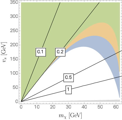
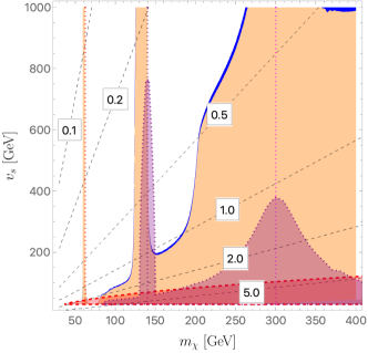
In FIG. 1, we show the constraint in the plane for and a few choices of . The colored region is allowed by the invisible decay constraint. The small gray region at the bottom of the plot denotes the region where and violates the perturbativity bound. The mixing angle has a significant impact on the constraints when is close to , in which region the phase space suppression becomes prominent. If contains more CP-even component, i.e., becomes larger, then the allowed phase space also becomes larger due to the extra factor of .
Next we consider the constraints coming from the measured Higgs signal strengths Zyla et al. (2020) listed in TABLE. 2.
| Channel | Signal Strength |
|---|---|
In the model, the couplings of to the other SM fields are modified universally by a factor of , leading to a reduction in the production rate by . The branching ratios, however, remains the same unless new invisible decay channel opens up when . The strongest bound comes from the slightly enhanced signal strength in , which at 95% C.L. requires
| (19) |
On the other hand, if is kinematically allowed, then the signal strengths of the SM channels are modified to be
| (20) |
where is the total decay width of the 125-GeV Higgs predicted by the SM. Seeing that such modifications would make the constraint on even stronger, we do not consider this case and only explore the case of in the benchmark studies, where we fix .
III.2 Electroweak Oblique Corrections
We now consider the Peskin-Takeuchi and parameters defined in Ref. Peskin and Takeuchi (1992). The current fits given by PDG Zyla et al. (2020) are
| (21) | ||||
with a correlation of . In our model, because the vector bosons only couple to the physical scalars through their -components, the mixing of which is determined entirely by and as shown in Eq. (10)777 only parametrizes the mixing between and , but not the gauge couplings, and hence does not take part in the oblique corrections., and parameters only depend on and, to a much less extent, . We fix as in Sec. III.1, and choose two sets of heavy scalar masses:
| (22) | ||||
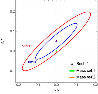
The first set is chosen to allow the , , and decays, while the second further allows the decay. For both mass sets, the above constraint can be satisfied within for all possible values of . In fact the oblique corrections have very little dependence on , whose contributions are suppressed by . We show the 68% C.L. and 95% C.L. contours in the - plane, as well as the values for both sets of masses, in FIG. 2. The detailed formulas for the electroweak oblique observables are given in Appendix B.
III.3 LHC Searches for Heavy Scalars
Here we consider constraints from direct searches of heavy neutral scalars at the LHC, focusing on the diboson final states: , and . The channel is less stringent. The light decay channels such as , , and are also less stringent because of suppressed decay BRs. 888Unlike in the C2HDM, we do not have to consider , , decays, which are absent in our model because the singlet scalar does not contain any “eaten” Goldstone bosons.
Because the singlet scalar does not couple to the SM gauge bosons and fermions directly, and couple to the SM gauge bosons and fermions only through their component. As such, their productions will go through the gluon-fusion (ggF) channel and are suppressed by the alignment parameter :
| (23) | ||||
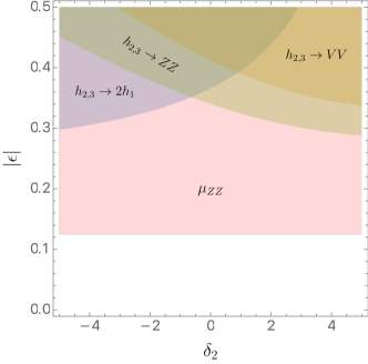
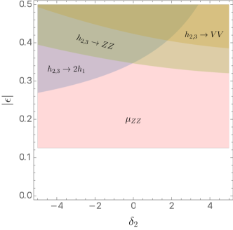
where , , and . In addition, and denote the SM production rate and decay partial width at the mass , which we obtain from Ref. de Florian et al. (2016). In addition to direct two-body decays from , we also include Higgs-to-Higgs decays such as .
We base our constraints on those in Refs. Aaboud et al. (2019b, 2018a); Sirunyan et al. (2018a); Aaboud et al. (2019c); Sirunyan et al. (2018b); Aaboud et al. (2018b, c); Sirunyan et al. (2019b); Aaboud et al. (2019d); Sirunyan et al. (2018c, 2019c); Aad et al. (2020a); Sirunyan et al. (2018d, 2020); Aad et al. (2020b, 2021). As seen in Eq. (23), the direct search constraints are all sensitive to , which suppresses the production rates by a factor of . Moreover, while the and constraints only depend on and in addition to and , the constraints further depend on , , and through their participation in the and couplings. Moreover, always shows up in and in the combination of , as can be seen in Eq. (15). We choose to fix and focus on the effects of on the constraints. In order to maximize the cross sections, we further maximize by choosing . Finally, we choose in a way that the ggF production rates of and are similar, which implies for the first mass set and for the second mass set in Eq. (22).
(a) (b)


(c) (d)
We examine the direct search constraints in the - plane for the two mass sets, and in the - plane with and , respectively, focusing on the region where , GeV, and . For definiteness as well as to impose the constraints on the parameter space in the strictest manner, we also neglect the decays. We present the results in FIG. 3, where we also include the constraint at 95% C.L. in Eq. (19). Note that in FIGS. 3(c) and (d), there are two sudden jumps caused by the onset of the decay when . It can be seen that the direct search constraints are all less stringent than the constraint, and thus for our choice of , both mass sets are completely safe from the LHC direct search constraints within the specified region.
III.4 Comments on electron EDM Constraints
We remark in this section that our CPVDM model does not generate new EDM contributions up to at least two-loop level, in sharp contrast with the C2HMDs. This is mainly due to the fact that new sources of CPV in our model are confined to the scalar and dark sectors: the CPV interactions take place among the scalars, or between and the messenger scalar . There is no new source of CPV in the visible fermionic sector as the singlet scalar does not have Yukawa interactions with the SM fermions. Therefore, even though the 125-GeV SM-like Higgs could have a component in due to the mass mixing, such a component does not introduce any CP-odd coupling of the 125-GeV Higgs to the SM fermions. Similar consideration applies to the heavy scalars couplings to SM fermions, which are induced only through the doublet component and remain CP-even. This explains why no electron EDM appears at one loop.


(a) (b)


(c) (d)
Now we exhibit potential two-loop contributions to coupling in our model in FIG. 4. To introduce CPV into the three-point electron-photon interaction, we must insert at least one trilinear/quartic CPV scalar vertex or one CPV scalar- vertex into the internal loops. In the first case, the scalars have to either all attach to the electron lines, such as that in FIG. 4(a), or form an internal loop, such as that in FIGS. 4(b) and (c). As for the second case, since only interacts with the scalars, it must form an internal loop, as shown in FIG. 4(d). For the cases of FIGS. 4(a), (b), and (c), no factor of would appear, and hence no EDM would be induced. As to FIG. 4(d), after taking the Dirac trace of the fermion loop, no Lorentz-invariant terms of the form would be induced, where is the rank-four Levi-Civita symbol and are generic four-momenta, and hence there is no EDM contribution either.
III.5 Muon Anomalous Magnetic Dipole Moment
In this section, we briefly comment on the contributions to the muon anomalous magnetic dipole moment, , in our model. The latest measurement was made in the E989 experiment at Fermilab, and the result was given by Abi et al. (2021)
| (24) |
while the SM prediction is given by Aoyama et al. (2020)
| (25) |
leading to a 4.2 discrepancy
| (26) |
The leading contributions are the one-loop diagrams and the two-loop Barr-Zee diagrams with top-, bottom-, -, and -loops running in the loop, as demonstrated in FIG. 5. Denoting their contributions by and , respectively, we have Ilisie (2015); Chen et al. (2020); Chiang and Yagyu (2021); Chen et al. (2021)
| (27) |
| (28) | ||||
where , , and
| (29) |
Note that they are both suppressed by . With the two chosen scalar mass sets, we have , which is negligible compared to Eq. (26). Thus, cannot be addressed in our model.


(a) (b)
III.6 DM Constraints: Relic Density, Direct and Indirect Searches

(a) (b)

(a) (b)
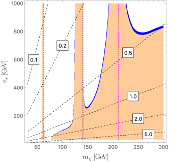
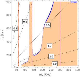
The DM relic density is measured to be Ade et al. (2016). The annihilation processes are shown in FIG. 6. We use micrOMEGAs Belanger et al. (2006, 2007, 2009, 2010, 2014) to calculate the relic density of , which is mainly determined by and . Other input parameters such as do not have a significant impact on the constraints. In FIG. 7 we show the relic density constraints in the - plane for the two mass sets mentioned in Eq. (22) with . The small blue regions denote the parameter space that has a relic density within the experimental 2 bounds, and the orange regions those below the lower 2 bound. We also plot the contour (red dotted), the contour (purple dotted), and the contour (magenta dotted) to show the resonance effect.
As can be seen in FIG. 7, the annihilation process is quite efficient for a DM mass that is sufficiently heavy, GeV, and/or small . In particular, a small increases for a fixed , which makes the annihilation rate larger. When the DM mass is close to the resonance region, , , the annihilation rate becomes enhanced and the relic density reduced, as can be seen from the plot. For our benchmark study, we choose the following four DM masses: GeV, which will be further studied in Sec. IV.
As for the DM direct searches, we quote the results of XENON1T Aprile et al. (2018). Since is only relevant to scalar interactions, it does not have a significant impact on the DM-nucleon scattering at the leading order. Furthermore, both scalar mass sets in Eq. (22) give roughly the same results. In FIG. 8(a), we show the experimental constraint in the - plane for mass set 1 and , taking the average of the spin-independent DM-proton and -neutron scattering cross sections.
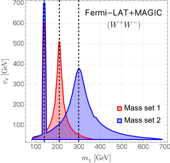
Finally, for indirect DM searches, we quote the results of the Fermi-LAT+MAGIC combined analysis Ahnen et al. (2016) to constrain dark matter annihilation in the and channels. In the channel we use the recent results given by MAGIC Acciari et al. (2021). We perform a scan over for the -pair annihilation rates into different final states. The dominant annihilation channel is largely determined by kinematics: for GeV, -pairs mainly annihilate into ; for GeV, they mainly annihilate into or ; for GeV, they mainly annihilate into heavy scalars, and occasionally to or .
Again does not have a considerable impact for annihilations into the SM particles, and we find the and constraints are always satisfied. In FIG. 8(b) we show the constraint in the - plane for the two scalar mass sets in Eq. (22). As shown in the plot, the indirect detection constraints are mostly caused by heavy scalar resonances near GeV (black dashed lines).
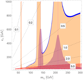
Before concluding this section, we summarize the DM relic, direct, and indirect detection constraints in FIG. 9.
(a) (b)
IV Triple and Quadruple Higgs Productions at the LHC
After considering current experimental constraints on our model, in this section we propose four benchmarks and consider their collider phenomenology at the 14-TeV LHC. To reduce the number of free parameters, we turn off the cubic couplings for , and in Eq. (1). We choose to focus on the possibility that is mostly CP-even and mostly CP-odd, which can be achieved by setting . With this parameter choice, is completely determined and we are free to set . In this scenario, CPV takes place in the Higgs-to-Higgs decays in the final state through the coupling and in the final state through the coupling, as can be seen from Eq. (15).999We could consider the other scenario where is mostly CP-even and is mostly CP-odd. In this case the terms proportional to in could be cancelled by properly choosing and , leading to similar decay characteristics. Therefore, the triple and quadruple Higgs productions at the LHC could be smoking gun signatures of CPV in the model.
In Table 3 we propose the four benchmark scenarios, {BP1, BP2, BP3, BP4}, to further study the signatures at the LHC. These four benchmarks have different collider phenomenology: BP1 and BP3 are chosen to allow the the production, while BP2 and BP4 are chosen to afford both the and productions. They satisfy all experimental constraints considered in previous sections. We fix all the parameters except , so as to look for regions of parameter space which maximize the event rates of final states. In this regard, we need to suppress the decays by choosing the appropriate and , resulting in interesting interplay with the DM relic density which we explain as follows.
| BP1 | BP3 | BP2 | BP4 |
| GeV, , , , | |||
| GeV, , | GeV, , | ||
| GeV, GeV | GeV, GeV | GeV, GeV | GeV, GeV |
| Free Parameter: | |||
In BP1 and BP2, we choose somewhat heavier DM masses, GeV for BP1 and (420, 200) GeV for BP2, both of which are heavier than in their respective benchmarks so that decays are forbidden and the Higgs-to-Higgs decay branching fractions are maximized. However, in this case pairs annihilate efficiently into (94%) and (4%), resulting in a vanishingly small relic density:
| (30) |
Other DM candidates (such as the axions) need to be present in these two benchmarks to satisfy the relic density. It is possible to choose benchmarks which fully account for the DM relic density with lighter DM masses, and they are presented in BP3 and BP4, where we choose GeV for BP3 and (156, 200) GeV for BP4. In BP3, pairs mainly annihilate to (61%), (28%), and (8%), while in BP4, they mainly annihilate to (61%), (27%), and (12%), giving the DM relic densities
| (31) |
(a) (b)


(c) (d)


(e) (f)
The production of the heavy scalars at the 14-TeV LHC goes through the ggF channel and the cross-sections are
| (32) | ||||
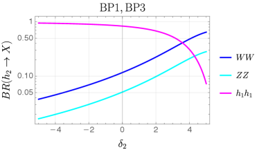
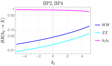
where we have chosen the values in such a way that the cross sections for and are the same, as mentioned in Sec. III.3. The decay branching ratios (BRs) of the heavy scalars are plotted against , the only free parameter in our benchmarks, in FIG. 10. We note that the decay BRs of in BP3 are the same as those in BP1, and those in BP4 the same as those in BP2. This is because the decay remains forbidden in BP3 and BP4 and the partial widths of other decay channels remain unchanged. Furthermore, as long as the scalar mixing angles are fixed, the decay partial widths of the are also fixed in the benchmarks.
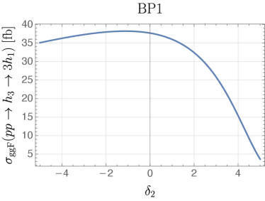
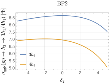
Given the production cross-sections and the decay BRs, we show in FIG. 11 the event rate of final states as a function of . In BP1/BP3, the maximum event rates for the are obtained for and , respectively, while in BP2/BP4, the maximum rates for and final states take place under different conditions. Maximizing the rate leads to in BP2 and in BP4. To summarize,
| (33) |
(a) (b)


(c) (d)
With event rates for and around and fb, respectively, it is imperative to dedicate experimental efforts to search for these final states at the 14-TeV LHC.
V Conclusions
In this work we have proposed a simple model of CP violation and dark matter, where the dark matter is a vector-like “dark fermion” which interacts with the SM only through a messenger scalar that is an electroweak singlet. New sources of CPV arise in the most general potential for the Higgs doublet and the singlet as well as the dark Yukawa coupling between and the dark matter. We have shown that such a simple setup could satisfy all current experimental constraints: Higgs signal strength measurements and searches for new neutral scalars at the LHC, precision electroweak measurements, electron EDM constraints, DM relic density, and DM direct and indirect detections. Notably, there is no new contributions to the electron EDM up to the two-loop level due to the fact that there is no new sources of CPV entering the visible fermion sector.
Novel signatures of CPV in this model come from Higgs-to-Higgs decays, , which involves a CPV coupling and does not vanish even in the exact alignment limit when the 125-GeV Higgs is exactly SM-like, in sharp contrast to the C2HDMs where the corresponding coupling becomes zero in the alignment limit. Moreover, the Higgs-to-Higgs decays, which include and , can give rise to yet-to-be-searched-for final states such as triple and quadruple 125-GeV Higgs bosons, which are highly suppressed within the SM. There is also no anomalous couplings in the Higgs sector, since is a singlet and does not couple to SM fermions. Only the 125-GeV Higgs coupling strengths are reduced due to the mass mixing.
While the and final states are smoking-gun signatures of CPV in the model (and in C2HDMs as well), it is conceivable that more complicated extensions of the SM without CPV, such as 2HDMs with an additional real singlet scalar, could also give rise to similar final states. In this regard, we point out that these more complicated extensions require the presence of additional neutral or charged scalars that are not present in the CPV models, which could be used to distinguish the models. Furthermore, it may be possible to unambiguously detect the presence of CPV trilinear scalar couplings through interference effects in the three-body decay as described in Ref. Chen et al. (2014), by considering the SM production of interfering with in the off-shell region, which is beyond the scope of the present work. It would also be interesting to consider ways to detect the CPV in the dark Yukawa coupling via, for example, directional direct detection.
Whether this model can accommodate the observed baryon asymmetry in the Universe remains to be seen. The feature that new sources of CPV are associated with interactions of the messenger scalar with the dark matter and the Higgs boson may indicate a connection between the proximity between the observed baryon relic abundance and the dark matter relic abundance Kaplan (1992); Kitano and Low (2005); Kaplan et al. (2009).
We hope it is clear that our work opens up a new frontier of searching for multi-Higgs bosons at the LHC. A detailed study on the discovery potential of the final states at the LHC is obviously necessary, which we plan to pursue in the future.
Acknowledgments
We thank Marcela Carena, Jia Liu, Carlos Wagner and Xiaoping Wang for their comments on the manuscript. We also acknowledge helpful discussions with Xiaoping Wang on the EDM constraint issues. IL would like to thank the support and the hospitality of the Physics Division of National Center for Theoretical Sciences (NCTS), Taiwan, where this project was initiated. TKC was supported in part by the grant of NCTS. CWC was supported in part by the Ministry of Science and Technology, Taiwan under the Grant No. MOST-108-2112-M-002-005-MY3. IL is supported in part by the U.S. Department of Energy under contracts No. DE- AC02-06CH11357 at Argonne and No. DE-SC0010143 at Northwestern.
Appendix A List of Couplings
We list in this appendix the trilinear and quartic scalar couplings as well as the couplings of the scalar fields to the SM fermions and weak gauge bosons in the model:
-
•
Trilinear Couplings:
(34) (35) (36) (37) (38) (39) (40) (41) (42) (43) -
•
Quartic Couplings:
(44) (45) (46) (47) (48) (49) (50) (51) (52) (53) (54) (55) (56) (57) (58) where , .
-
•
Couplings of Scalar Fields to SM Fermions and Gauge Bosons:
(59) (60) (61)
Appendix B Formulae for Electroweak Oblique Corrections
The scalar contributions to and are given by
| (62) | ||||
where
| (63) |
| (64) |
and
| (65) |
References
- Barger et al. (2009) V. Barger, P. Langacker, M. McCaskey, M. Ramsey-Musolf, and G. Shaughnessy, Phys. Rev. D 79, 015018 (2009), arXiv:0811.0393 [hep-ph] .
- Chiang and Senaha (2008) C.-W. Chiang and E. Senaha, JHEP 06, 019 (2008), arXiv:0804.1719 [hep-ph] .
- Alexander-Nunneley and Pilaftsis (2010) L. Alexander-Nunneley and A. Pilaftsis, JHEP 09, 021 (2010), arXiv:1006.5916 [hep-ph] .
- Barger et al. (2010) V. Barger, M. McCaskey, and G. Shaughnessy, Phys. Rev. D 82, 035019 (2010), arXiv:1005.3328 [hep-ph] .
- Gonderinger et al. (2012) M. Gonderinger, H. Lim, and M. J. Ramsey-Musolf, Phys. Rev. D 86, 043511 (2012), arXiv:1202.1316 [hep-ph] .
- Gabrielli et al. (2014) E. Gabrielli, M. Heikinheimo, K. Kannike, A. Racioppi, M. Raidal, and C. Spethmann, Phys. Rev. D 89, 015017 (2014), arXiv:1309.6632 [hep-ph] .
- Jiang et al. (2016) M. Jiang, L. Bian, W. Huang, and J. Shu, Phys. Rev. D 93, 065032 (2016), arXiv:1502.07574 [hep-ph] .
- Darvishi and Krawczyk (2021) N. Darvishi and M. Krawczyk, Nucl. Phys. B 962, 115 (2021), arXiv:1603.00598 [hep-ph] .
- Darvishi and Masouminia (2017) N. Darvishi and M. R. Masouminia, Nucl. Phys. B 923, 491 (2017), arXiv:1611.03312 [hep-ph] .
- Chiang et al. (2018) C.-W. Chiang, M. J. Ramsey-Musolf, and E. Senaha, Phys. Rev. D 97, 015005 (2018), arXiv:1707.09960 [hep-ph] .
- Chiang and Lu (2020) C.-W. Chiang and B.-Q. Lu, JHEP 07, 082 (2020), arXiv:1912.12634 [hep-ph] .
- Robens et al. (2020) T. Robens, T. Stefaniak, and J. Wittbrodt, Eur. Phys. J. C 80, 151 (2020), arXiv:1908.08554 [hep-ph] .
- Ivanov (2017) I. P. Ivanov, Prog. Part. Nucl. Phys. 95, 160 (2017), arXiv:1702.03776 [hep-ph] .
- Carena et al. (2014) M. Carena, I. Low, N. R. Shah, and C. E. M. Wagner, JHEP 04, 015 (2014), arXiv:1310.2248 [hep-ph] .
- Carena et al. (2015) M. Carena, H. E. Haber, I. Low, N. R. Shah, and C. E. M. Wagner, Phys. Rev. D 91, 035003 (2015), arXiv:1410.4969 [hep-ph] .
- Carena et al. (2016) M. Carena, H. E. Haber, I. Low, N. R. Shah, and C. E. M. Wagner, Phys. Rev. D 93, 035013 (2016), arXiv:1510.09137 [hep-ph] .
- Grzadkowski et al. (2014) B. Grzadkowski, O. M. Ogreid, and P. Osland, JHEP 11, 084 (2014), arXiv:1409.7265 [hep-ph] .
- Grzadkowski et al. (2018) B. Grzadkowski, H. E. Haber, O. M. Ogreid, and P. Osland, JHEP 12, 056 (2018), arXiv:1808.01472 [hep-ph] .
- Kanemura et al. (2020) S. Kanemura, M. Kubota, and K. Yagyu, JHEP 08, 026 (2020), arXiv:2004.03943 [hep-ph] .
- Low et al. (2020) I. Low, N. R. Shah, and X.-P. Wang, (2020), arXiv:2012.00773 [hep-ph] .
- Bento et al. (1991) L. Bento, G. C. Branco, and P. A. Parada, Phys. Lett. B 267, 95 (1991).
- Branco et al. (2003) G. Branco, P. Parada, and M. Rebelo, (2003), arXiv:hep-ph/0307119 .
- Costa et al. (2015) R. Costa, A. P. Morais, M. O. P. Sampaio, and R. Santos, Phys. Rev. D 92, 025024 (2015), arXiv:1411.4048 [hep-ph] .
- Darvishi (2016) N. Darvishi, JHEP 11, 065 (2016), arXiv:1608.02820 [hep-ph] .
- Sirunyan et al. (2019a) A. M. Sirunyan et al. (CMS), Phys. Lett. B 793, 520 (2019a), arXiv:1809.05937 [hep-ex] .
- Aaboud et al. (2019a) M. Aaboud et al. (ATLAS), Phys. Rev. Lett. 122, 231801 (2019a), arXiv:1904.05105 [hep-ex] .
- Zyla et al. (2020) P. A. Zyla et al. (Particle Data Group), PTEP 2020, 083C01 (2020).
- Peskin and Takeuchi (1992) M. E. Peskin and T. Takeuchi, Phys. Rev. D 46, 381 (1992).
- de Florian et al. (2016) D. de Florian et al. (LHC Higgs Cross Section Working Group), 2/2017 (2016), 10.23731/CYRM-2017-002, arXiv:1610.07922 [hep-ph] .
- Aaboud et al. (2019b) M. Aaboud et al. (ATLAS), JHEP 05, 124 (2019b), arXiv:1811.11028 [hep-ex] .
- Aaboud et al. (2018a) M. Aaboud et al. (ATLAS), Eur. Phys. J. C 78, 1007 (2018a), arXiv:1807.08567 [hep-ex] .
- Sirunyan et al. (2018a) A. M. Sirunyan et al. (CMS), JHEP 01, 054 (2018a), arXiv:1708.04188 [hep-ex] .
- Aaboud et al. (2019c) M. Aaboud et al. (ATLAS), JHEP 04, 092 (2019c), arXiv:1811.04671 [hep-ex] .
- Sirunyan et al. (2018b) A. M. Sirunyan et al. (CMS), Phys. Lett. B 778, 101 (2018b), arXiv:1707.02909 [hep-ex] .
- Aaboud et al. (2018b) M. Aaboud et al. (ATLAS), Phys. Rev. Lett. 121, 191801 (2018b), [Erratum: Phys.Rev.Lett. 122, 089901 (2019)], arXiv:1808.00336 [hep-ex] .
- Aaboud et al. (2018c) M. Aaboud et al. (ATLAS), JHEP 11, 040 (2018c), arXiv:1807.04873 [hep-ex] .
- Sirunyan et al. (2019b) A. M. Sirunyan et al. (CMS), Phys. Lett. B 788, 7 (2019b), arXiv:1806.00408 [hep-ex] .
- Aaboud et al. (2019d) M. Aaboud et al. (ATLAS), JHEP 01, 030 (2019d), arXiv:1804.06174 [hep-ex] .
- Sirunyan et al. (2018c) A. M. Sirunyan et al. (CMS), JHEP 08, 152 (2018c), arXiv:1806.03548 [hep-ex] .
- Sirunyan et al. (2019c) A. M. Sirunyan et al. (CMS), Phys. Rev. Lett. 122, 121803 (2019c), arXiv:1811.09689 [hep-ex] .
- Aad et al. (2020a) G. Aad et al. (ATLAS), Phys. Lett. B 800, 135103 (2020a), arXiv:1906.02025 [hep-ex] .
- Sirunyan et al. (2018d) A. M. Sirunyan et al. (CMS), JHEP 06, 127 (2018d), [Erratum: JHEP 03, 128 (2019)], arXiv:1804.01939 [hep-ex] .
- Sirunyan et al. (2020) A. M. Sirunyan et al. (CMS), JHEP 03, 034 (2020), arXiv:1912.01594 [hep-ex] .
- Aad et al. (2020b) G. Aad et al. (ATLAS), Eur. Phys. J. C 80, 1165 (2020b), arXiv:2004.14636 [hep-ex] .
- Aad et al. (2021) G. Aad et al. (ATLAS), Eur. Phys. J. C 81, 332 (2021), arXiv:2009.14791 [hep-ex] .
- Abi et al. (2021) B. Abi et al. (Muon g-2), Phys. Rev. Lett. 126, 141801 (2021), arXiv:2104.03281 [hep-ex] .
- Aoyama et al. (2020) T. Aoyama et al., Phys. Rept. 887, 1 (2020), arXiv:2006.04822 [hep-ph] .
- Ilisie (2015) V. Ilisie, JHEP 04, 077 (2015), arXiv:1502.04199 [hep-ph] .
- Chen et al. (2020) K.-F. Chen, C.-W. Chiang, and K. Yagyu, JHEP 09, 119 (2020), arXiv:2006.07929 [hep-ph] .
- Chiang and Yagyu (2021) C.-W. Chiang and K. Yagyu, Phys. Rev. D 103, L111302 (2021), arXiv:2104.00890 [hep-ph] .
- Chen et al. (2021) C.-H. Chen, C.-W. Chiang, and T. Nomura, Phys. Rev. D 104, 055011 (2021), arXiv:2104.03275 [hep-ph] .
- Ade et al. (2016) P. A. R. Ade et al. (Planck), Astron. Astrophys. 594, A13 (2016), arXiv:1502.01589 [astro-ph.CO] .
- Belanger et al. (2006) G. Belanger, F. Boudjema, A. Pukhov, and A. Semenov, Comput. Phys. Commun. 174, 577 (2006), arXiv:hep-ph/0405253 .
- Belanger et al. (2007) G. Belanger, F. Boudjema, A. Pukhov, and A. Semenov, Comput. Phys. Commun. 176, 367 (2007), arXiv:hep-ph/0607059 .
- Belanger et al. (2009) G. Belanger, F. Boudjema, A. Pukhov, and A. Semenov, Comput. Phys. Commun. 180, 747 (2009), arXiv:0803.2360 [hep-ph] .
- Belanger et al. (2010) G. Belanger, F. Boudjema, A. Pukhov, and A. Semenov, Nuovo Cim. C 033N2, 111 (2010), arXiv:1005.4133 [hep-ph] .
- Belanger et al. (2014) G. Belanger, F. Boudjema, A. Pukhov, and A. Semenov, Comput. Phys. Commun. 185, 960 (2014), arXiv:1305.0237 [hep-ph] .
- Aprile et al. (2018) E. Aprile et al. (XENON), Phys. Rev. Lett. 121, 111302 (2018), arXiv:1805.12562 [astro-ph.CO] .
- Ahnen et al. (2016) M. L. Ahnen et al. (MAGIC, Fermi-LAT), JCAP 02, 039 (2016), arXiv:1601.06590 [astro-ph.HE] .
- Acciari et al. (2021) V. A. Acciari et al. (MAGIC), (2021), arXiv:2111.15009 [astro-ph.HE] .
- Chen et al. (2014) Y. Chen, A. Falkowski, I. Low, and R. Vega-Morales, Phys. Rev. D 90, 113006 (2014), arXiv:1405.6723 [hep-ph] .
- Kaplan (1992) D. B. Kaplan, Phys. Rev. Lett. 68, 741 (1992).
- Kitano and Low (2005) R. Kitano and I. Low, Phys. Rev. D 71, 023510 (2005), arXiv:hep-ph/0411133 .
- Kaplan et al. (2009) D. E. Kaplan, M. A. Luty, and K. M. Zurek, Phys. Rev. D 79, 115016 (2009), arXiv:0901.4117 [hep-ph] .
- Aguilar-Saavedra et al. (2020) J. A. Aguilar-Saavedra, J. Alonso-González, L. Merlo, and J. M. No, Phys. Rev. D 101, 035015 (2020), arXiv:1911.10202 [hep-ph] .
- Barbieri et al. (2004) R. Barbieri, A. Pomarol, R. Rattazzi, and A. Strumia, Nucl. Phys. B 703, 127 (2004), arXiv:hep-ph/0405040 .