A simple demonstration of shear-flow instability.
Abstract
We describe a simple classroom demonstration of a fluid-dynamic instability. The demonstration requires only a bucket of water, a piece of string and some used tealeaves or coffee grounds. We argue that the mechanism for the instability, at least in its later stages, is two-dimensional barotropic (shear-flow) instability and we present evidence in support of this. We show results of an equivalent basic two-dimensional numerical non-linear model, which simulates behavior comparable to that observed in the bucket demonstration. Modified simulations show that the instability does not depend on the curvature of the domain, but rather on the velocity profile.
Videos
The manuscript cites video clips which are available password-protected on the vimeo video-sharing site. We strongly encourage readers to watch these video clips, in particular the following two, as they add a lot to the description given by the text and figures.
The experiment: VideoS1 available at https://vimeo.com/278481176 (password: Welcome123)
The numerical simulation (slow motion): VideoS2 available at https://vimeo.com/399593365 (password: Welcome123),
This article may be downloaded for personal use only. Any other use requires prior permission of the author and AIP Publishing. This article appeared in American Journal of Physics 88, Issue 12, 1041 (2020) and may be found at https://doi.org/10.1119/10.0002438
I Introduction
Shear-flow instability is a fundamental process in fluid dynamics, and is associated with the destruction of parallel laminar flow. As such, it can be seen as fundamental to the onset and existence of both two- and three-dimensional turbulence.(e.g. phillips1969shear, ) Geophysicists usually use the term “barotropic instability” in the context of the instability of a horizontally-sheared fluid on a rotating planet. The word “barotropic” distinguishes this from baroclinic instability, in which horizontal temperature gradients play a key role. Baroclinic instability is the major large-scale weather-generating process of the mid-latitudes (the region between the tropics and the polar circles), whereas barotropic instability is important as an instability mechanism for jets and vortices. Both instabilities may be associated with the polygonal shapes often observed in the atmospheres of rotating planets.(e.g. Kossin, ; Adriani, )
The instructional value of laboratory demonstrations is well-recognized, both in the context of geophysical fluid dynamics in particular,Illari ; Marshall ; mackin2012effectiveness and in the context of fluid dynamics in general (Shakerinshakerin2018fluids and references therein). A classroom demonstration (e.g. BIVideo ) of baroclinic instability can be prepared based on the “dishpan” experiments of the mid-twentieth century.(e.g. Fultz, ) To study barotropic instability in the laboratory, sophisticated experiments somewhat analogous to the dishpan experiments can be constructed using differentially rotating boundaries.(e.g. Aguiar, ; Konijnenberg, ; Nezlin, ) The shear is introduced due to the differential rotation of concentric sections of the bottom of the container of the working fluid. However, such an apparatus is beyond the budget of most classroom teaching of geophysical fluid dynamics.
Reynolds Reynolds describes experiments with a horizontal glass tube containing carbon disulphide overlain by water. Carbon disulphide is a highly toxic liquid with a density approximately 25% higher than water at room temperature. By tilting the tube, Reynolds induced a counterflow in the two liquids and this led to instability at the shear interface when the velocity difference was large enough. A version of this apparatus, using a carefully-established saline/fresh water step to create the density difference, is a well-loved teaching aid at the University of Cambridge.KHVideo However, the equipment is quite specialized and the set-up procedure is painstaking and time-consuming. One simpler classroom option is to introduce shear by moving a solid boundary through a fluid — for example a cylinder with vertical axis, partially submerged in water, may be towed sideways. Food dye applied to the cylinder before immersion, or mica powder mixed into the water, exposes the vortices which appear in the wake. Kelley and Ouellettekelley describe a laboratory approach aimed at undergraduate students, who use an electromagnetic technique to drive Kolmogorov flow (a type of cyclic shear flow which exhibits shear-flow instability under some forcing parameters) in a thin fluid layer, and measure it quantitatively with a webcam. The authors estimate costs of the order of $ 500. Vorobieff and Eckevorobieff1999fluid present an apparatus based on a tilted gravity-driven soap tunnel, with which a variety of fluid-dynamic phenomena, including shear instability, can be demonstrated. Their estimated costs were of the order of $1000 (in 1999).
Here we describe an instance of an instability that can be easily reproduced in a bucket and used as a very low-budget demonstration, which we have found to engage a wide range of student groups. We argue that the instability, at least in its later stages, is consistent with the two-dimensional shear flow instability exhibited by a basic numerical model.
II Brief review of the mechanism of shear-flow instability
To introduce the mechanism we begin with a two-dimensional conceptual model consisting of two regions of incompressible fluid of constant uniform density (let’s call them the North and South parts) each in uniform flow in opposite directions like two counterflowing carriageways of traffic. Nothing divides them; their interface is initially a straight vertical plane. For simplicity in this section we do not consider a curved shear layer as seen in the bucket. We show in subsection IV.3 that the curvature is not an essential feature of our demonstration.
The fundamental cause of shear flow instability is this: interaction of the two parts can exchange momentum between them and release kinetic energy, which is then available to drive a more complex (sometimes chaotic) behavior in the region of the interface.
The details of the mechanism are most easily understood in terms of a derived property of fluid motion called vorticity. Mathematically, vorticity is the curl of the velocity field. In a two-dimensional flow context, we can regard the vorticity as a scalar, because its direction is always the same (normal to the plane of the motion). Shapiroshapirovideo offers a striking physical interpretation of vorticity, which we paraphrase here: “The vorticity is a measure of the moment of momentum of a small fluid particle about its center of mass. Suppose that you had some very complicated [two-dimensional] motion in a liquid and that it were possible by magic suddenly to freeze a small sphere of that liquid into a solid. During the freezing the moment of momentum would be conserved. The vorticity of the fluid before freezing is exactly twice the angular velocity of the solid sphere just after its birth.” This vivid interpretation may sound fanciful, but the mental image it conjures is not so different from what we see in the development of shear-flow instability: vorticity (which is initially present as a continuous shear at the interface) is rapidly converted by the instability into the rotation of a number of vortices along the line of the interface.
The mechanism is illustrated in Fig. (1), which is adapted from Batchelor.batchelor1967 The process begins with undisturbed counterflow and a straight interface as described above, shown by the dashed straight line (this line would have a monotonic curve in the case of the bucket demonstration). We introduce a small sinusoidal disturbance as shown. It can be shown that disturbed vorticity south of the dashed line (for example at D) induces eastward movement in the vorticity north of the dashed line, and likewise vorticity north of the dashed line (for example at B) induces westward movement in the vorticity south of the dashed line. Both of these effects concentrate vorticity at points like A, giving a positive feedback, with energy provided by the kinetic energy of the counterflowing parts. The arrows indicate the direction of the movement of the vorticity induced by the disturbance, and show both the accumulation of vorticity at points like A (purple arrows) and the general rotation about points like A (red arrows) which together lead to growth of the disturbance. The accumulation of vorticity (at points like A) and depletion of vorticity (at points like C) is also indicated by the thickness of the wavy line. A comprehensive discussion of this case is given by Batchelor.batchelor1967
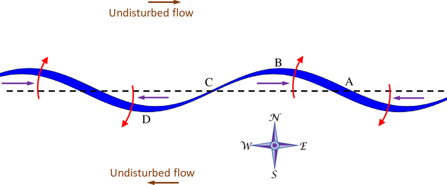
In this simplified configuration the sinusoidal disturbance grows around nodes (like point A for example) with fixed spatial locations where distinct vortices will, ultimately, form. Extending the traffic analogy, a typical vortex centre is like a fixed point on the road, with traffic sweeping past one way on one side, and the other way on the other side.
In a more general case where the velocities are not equal and opposite, for example in the demonstration which we describe next, the vortices move along the line of an interface at a speed intermediate between the faster-moving fluid on one side and the slower-moving fluid on the other side of the interface.
III Demonstration
III.1 Description
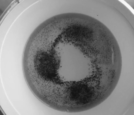
A bucket (ours has an internal diameter of 180 mm) is filled with tap water to a depth of about 30 mm. A few used tealeaves or coffee grounds are added as a simple flow tracer. A piece of string is attached to the center of the bucket handle and the bucket lifted a little so that it is suspended on the string. A vigorous angular impulse (a flick) is applied to the handle using the fingers, and the bucket allowed to spin for a few turns. This sets the water at and near the wall in rotation. The bucket is then set back down, arresting its rotation (and attenuating the motion of the water nearest to the wall). Typically, within a few seconds, the axisymmetry of the resulting flow breaks and a number of smaller vortices (typically two, three or four) appear — see Fig. (2) and our first video clip VideoS1, available at https://vimeo.com/278481176 (password: Welcome123). These smaller vortices, which rotate in the same sense as the initial rotation of the bucket, will typically merge into a near-axisymmetric single vortex in a few more seconds, before the motion dies completely. With careful observation, the vortices can also be seen on the top surface, for example by sprinkling buoyant glitter onto the water. However the tealeaves (which have a small negative buoyancy and thus illustrate the flow near the bottom boundary) have the well-recognized tendency to converge in the vortices,(tandon2010einstein, ) and this provides an impactful visualization. Incidentally, we came upon our demonstration by accident whilst playing with a version of the well-known “Einstein’s Tea Leaves” demonstration,(tealeavesfilm, ) which is widely used in teaching the behavior of air near the surface of atmospheric pressure systems.(tandon2010einstein, )
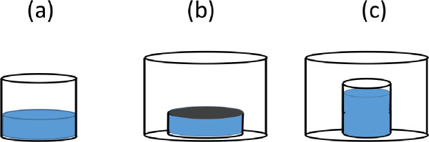
A snapshot of the demonstration is shown in Fig. (2). The initial flick was of the order of four revolutions per second and the rotation of the bucket was then arrested by replacing it on the table after about two seconds. However, the behavior seems to be quite robust to variations as long as the initial flick is strong enough. We have observed the instability in a taller, narrower configuration (120 mm diameter by 100 mm deep) and in a setup with a rigid lid, arranged by filling a transparent cylindrical plastic container (a cake box) with water, placing a larger bucket upside down over the box so that the base of the bucket forms a lid to the box, and then inverting the whole. Atmospheric pressure stops the water from draining out of the box (rather like a very squat manometer). Similar instability behavior is seen in each case. These alternative configurations are shown schematically in Fig. (3), and video clips of their behavior are linked from section VI.
III.2 Curricular Context
In a teaching context, this demonstration could, for example, be included in a session introducing the general behavior of the mid-latitude atmosphere via the concept of fluid-dynamic instability. The initial velocity profile (which is shown in Fig. (4)) can be interpreted as a jet, whose instability leads to the production of several vortices. Whilst this is a loose and incomplete model of the mid-latitudes, it does provide an engaging, hands-on approach. Given the low cost, it is easy to provide a group of students with several buckets so that they can experiment and observe the behavior in small groups. In the early 20th century barotropic and baroclinic instability were rival hypotheses for the explanation of the observed mid-latitude eddies,(James, ) and so having introduced the general concept of fluid-dynamic instability via the buckets, the session can then move on to a demonstration of baroclinic instability such as the one described by Marshall and Plumb.Marshall Alternatively, the activity could play a role in demystifying observations of polygonal patterns in the atmosphere of rotating planets.(e.g. Kossin, ; Adriani, )
III.3 Nature of the instability
When the bucket is arrested, the water in contact with the bucket is also arrested (in accordance with the no-slip condition). So now the depth-averaged azimuthal velocity reaches a peak near the wall but falls to zero at the wall.
As discussed by Rabaud and Couder,rabaud1983shear Colescoles1965transition observed patterns of “rollers” with their axes parallel to the rotation axis (Coles’ Fig. 22(o)) in a Couette geometry (concentric independently-rotating cylinders), associated with sudden starts and stops of the rotation of the outer cylinder, which created an inflection in the velocity profile. This description is strikingly similar to our experiment and observations.
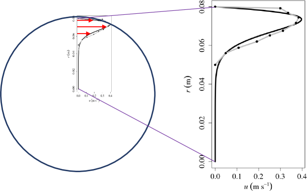
Our crudely-measured velocity profile, from before any visible onset of instability, is shown in Fig. (4). The velocity profile at this stage satisfies the Rayleigh-Kuo criterion,(andrews2010introduction, ) which is a necessary (though not sufficient) condition for shear-flow instability. In our context this criterion is that the velocity profile must include an inflection point, i.e. a point at which the curvature of the velocity profile changes sign.
In initial discussion with correspondents (see acknowledgments), various candidate processes were suggested for the observed instability, including centrifugal instability generating turbulence followed by an up-scale energy transfer; an instability of the Ekman layer; and shear instability. Cullen (pers. comm.) noted that the observed behavior appears to be quasi-two-dimensional, and that such flow would not be observed in the first place if it was unstable to three-dimensional disturbances. In the following section we show that a two-dimensional model (which admits no variation in the vertical direction) exhibits behavior similar to that observed when the model is initialized with a profile based on the measured profile of Fig. (4).
IV Numerical model
IV.1 Description
We describe a non-linear two-dimensional numerical model of the instability seen in the bucket. The stream function, , and vorticity, , are convenient tools for such a model. For our purpose, each is a scalar function of space and time. Mathematically, we define the stream function as a field, the 2-D Laplacian of which is the vorticity field. Physically, this gives the useful properties that the instantaneous contours of the stream function (which may be familiar to some readers as “streamlines”) are everywhere tangent to the instantaneous velocity vector, and that regions of rapid movement can be identified by closely-packed streamlines. The streamlines indicate the paths that particles in the flow would take if the flow did not evolve over time. In our case the flow does evolve over time, so the stream lines are not identical to particle paths (see VideoS3).
The values of stream function and vorticity do not depend on the coordinate system in which they are evaluated. For our purpose it is convenient to use a polar coordinate system: we use a polar grid with 256 azimuthal grid points and 112 radial grid points. The integration procedure is:
-
•
Given a vorticity field
-
•
Invert the Laplacian to obtain the stream function, , given in polar coordinates by , , where is azimuthal velocity component, is meridional (i.e. radial) velocity component, is radius and is the azimuthal angle (in radians, defined positive in the direction of increasing )
-
•
Evaluate the components of velocity from the gradient of the stream function
-
•
Advect the vorticity field for one time-step. “Advection” refers to movement by the flow of the fluid; thus in this context “advect” the vorticity means move the vorticity, using the velocity that we evaluated. We use a simple upwind explicit scheme with a small time-step to accomplish this.
-
•
Repeat
Inversion of the Laplacian is a linear problem that can be addressed by a Fourier decomposition in the azimuthal direction. Owing to the linearity, the modes can be treated independently. This requires one tri-diagonal matrix inversion for each mode.
We initialized our model with the smooth velocity profile shown by the black line in Fig. (4). This velocity is a heuristic analytical function of the radius, as follows: , where , is the outer radius, and are tunable parameters, being a scale width for the velocity jet. The fit was chosen by eye such that the peak azimuthal speed and the radius at which it occurred matched well with the measured profile. We used m, m s-1, . This gives a profile which is simple to work with, whilst maintaining consistency with the measurements to within their uncertainties. A more complicated alternative would be to use piecewise linear interpolation (as shown by the gray lines) between each of the measurements, but this seems unjustified given the uncertainties. The radial gradient of vorticity changes sign at about meters for our fitted profile, and somewhere between m and m for the measured profile.
We add a field of small random vorticity ‘noise’ to initialize any instability. Typical magnitudes (root-mean-square) of the noise are set to be of the order of 0.1% of typical values of the initial vorticity profile. To sidestep the difficulty with the singularity at the pole we truncate the grid at a small but non-zero radius and approximate the behavior of the fluid within this radius as a blob of material which is allowed to revolve in rigid rotation around the pole but is otherwise identical to the rest of the fluid. (We suggest that this is only a minor constraint on the motion, and we note that a version of the laboratory demonstration not shown here including a comparable fixed rigid central cylinder of mm diameter exhibits very similar instability behavior.) This leads naturally to a Neumann boundary condition on for the mode (which represents the average) of the stream function at the inner boundary:
| (1) |
since is the azimuthal velocity of the rigid circular blob. Konijnenberg et al. Konijnenberg use a similar boundary condition (their equation 5.8). For the other modes, we apply a Dirichlet boundary condition at the inner boundary:
| (2) |
which represents the constraint that no fluid can pass through the circular boundary of the rigid blob. At the outer boundary we apply a Dirichlet boundary condition to all modes (including ):
| (3) |
Again, for the mode, this represents the constraint that no fluid can pass through the outer circular boundary of the domain (the wall of the bucket), and in the case of the mode, this effectively sets the arbitrary zero for the stream function so that the solution is unique.
The inner boundary conditions for the vorticity are
Treating the circular blob as rigid implies that its vorticity has a single value at any time. Our implementation of Eq. (1) ensures that this vorticity is the average of the vorticity of the fluid just outside the blob (since the mode represents the average).
We do not include any explicit model of diffusion. Our first-order upwind scheme is known to be diffusive, and one might optimistically argue that this property of the two-dimensional numerical model mimics the damping influence of the bottom boundary in the bucket. However we have not made any quantitative comparison of these damping factors.
IV.2 Numerical modelling results and discussion
Summary: the modelled evolving flow exhibits instability which is visually similar to that observed in the bucket, when initialized with a velocity profile similar to that measured. The emergent modelled preferred wavenumber (which is three in this instance) is the same as that observed, and the modelled growth rate is consistent with that observed.
A common visualization tool for water flows is to add coloured dye to some parts of the water. The dye acts as a passive “tracer”: showing the movement without influencing the movement. In our physical demonstration the tea leaves perform a similar function, except that they tend to congregate in the vortices due to bottom boundary effects which are not simulated in our numerical model. It is relatively simple to add a simulation of a numerical passive tracer to the numerical model, and the result gives an intuitive sense of the behavior, because the tracer looks like phenomena which can be seen in the real world — for example the patterns seen in creamer added to coffee.
A video clip of the simulation, VideoS2, available at https://vimeo.com/399593365 (password: Welcome123), shows a slow motion (one-fifth speed) animation of some aspects of the simulation, concentrating on the most interesting period of flow evolution. The top left-hand panel shows our tracer. The tracer starts out as a sinusoidal pattern of 4 radial cycles and 7 azimuthal cycles We chose 7 cycles to ensure that we did not prejudice the visual emergence of three vortices. Green shows positive values of tracer and purple shows negative values of tracer. The tracer diffuses, so we reset it at about 4.5 seconds to capture the most interesting part of the evolution.
A alternative intuitive visualization is shown in the top right-hand panel: a cloud of dots moving with the flow. Physically these are analogous to paper dots floating on the surface of the water in the bucket. The initial positions of the dots are chosen randomly. A short “tail” shows the recent track of each dot. The passive tracer of the top left panel is shown again faintly in gray for comparison.
Neither the tracer nor the dots are subject to the process which tends to concentrate the tea leaves in the vortices in the physical demonstration, and the formation of three separate vortices is seen more clearly in an animation of the stream function, shown by color-filled contours in the bottom left panel. You can see that three sets of closed streamlines appear, corresponding to three vortices. Thus the three areas of closed streamlines correspond to the three areas in which the tea leaves tend to congregate in the physical experiment. The bottom right panel shows the dots with their “tails” again, this time overlain on contours of the stream function (streamlines). By watching this panel closely (and, if possible, stopping the animation after the three sets of closed streamlines have appeared and stepping through one frame at a time) you can see for yourself that the instantaneous movement of the particles is always along the streamlines, even though the particle paths are not identical to streamlines (because the streamlines evolve).
Video clip VideoS3, available at https://vimeo.com/279323035 (password: Welcome123), shows the evolution of the stream function in real time over the entire 30-second-long simulation. The sense of the imposed initial rotation was clockwise in both the physical demonstration and the simulation.
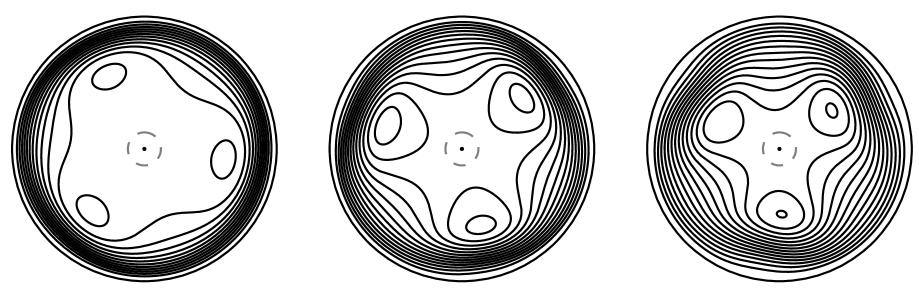
Figure (5) shows snapshots of the evolving simulated stream function after the instability has begun to grow.
To investigate the growth of the instability during a particular simulation we focus on the radial velocity at approximately the mid radius (about 45 mm). A Hovmoller diagram is a common way of plotting meteorological data. The axes are typically longitude or latitude (x-axis) and time (y-axis) with the value of some field represented through color or shading. Figure (6(a)) is a Hovmoller diagram of the radial velocity at mid radius, which illustrates the inception, growth, and advection (movement by the flow) of the vortices arising from the instability.
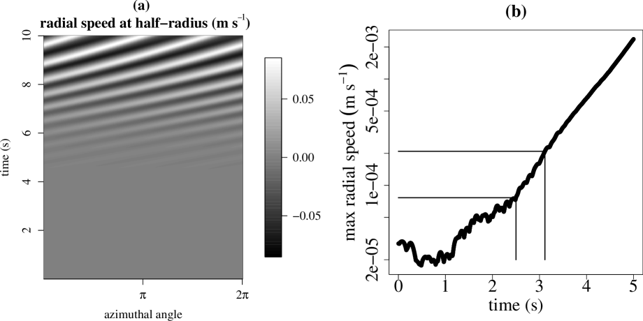
To estimate the growth rate of the modelled instability we use the maximum radial velocity at the mid radius as a simple metric of the strength of the instability. The evolution of this metric is shown in Fig. (6(b)). Choosing a small section of the steepest part of the curve (delineated by the straight lines on the plot) facilitates estimation of the growth rate. We find an e-folding time of approximately 0.6 seconds. Growth rates in the experiment and model can be visually compared by comparing the video clips; they appear similar. We do not have a precise measurement of the growth rate in the experiment, but the three vortices are well-established by time t=8.2 seconds on the video clip, unidentifiable at 6.2 seconds, and arguably detectable at around 7.2 seconds. These observations are not inconsistent with the e-folding time of 0.6 seconds obtained from the model.
The model is quite basic, perhaps even crude by contemporary standards. However, a two-dimensional linear stability analysis yields very similar results in terms of wavenumber and growth rate of the instability (see appendix B). The cross-corroboration of the three experiments (laboratory, numerical and analytical) gives confidence in the numerical model results, in spite of its simplicity, and supports our suggestion that the instability is fundamentally two-dimensional. The strong similarity between the behavior seen in the two-dimensional model and the observed behavior suggests that, although a centrifugal instability may be involved in the creation of the profile we measured, a two-dimensional process with negligible variation in the vertical direction — we suggest the barotropic (shear-flow) instability associated with the change in sign of the radial gradient of vorticity — can account for the evolution of the flow forwards in time from our axisymmetric measured profile.
IV.3 Modified numerical model: cyclic straight channel
The instability is also simulated when the curvature is artificially removed, modelling a hypothetical straight channel with cyclic lateral boundaries.
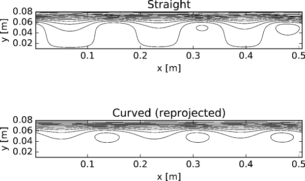
A well-recognized advantage of numerical modelling is the ease of modifying the experiment. To show that the existence of an instability depends on the velocity profile, and not on the curvature of the domain, we modified the numerical simulation. The modified simulation consists of a straight two-dimensional domain with cyclic boundaries in the primary () direction and walls bounding the other () direction. Thus the direction replaces the radial () direction of the previous simulation, and we choose the width (in the direction) of the domain to match the radius of the bucket. The velocity profile that was used to initialize the previous simulation is here the initial -direction velocity, and we choose the length (in the direction) of the domain to be approximately the circumference of the bucket (about 0.5 meters). We use a rectilinear grid in place of the polar grid of the previous simulation, and remove any of the terms describing effects associated with the curvature of the domain. In order to study the effect of only the removal of the curvature, we retain the cyclic lateral boundary conditions.
This simulation exhibits a similar instability to that seen in the curved simulation (see Fig. (7)).
The cyclic lateral boundaries create a periodic domain and this quantizes the allowable wavenumbers.(Vallis, ) We also performed a simulation with cyclic lateral boundaries and a doubled length (in the direction). The initial velocity profile remained unchanged. The double-length simulation exhibited an instability with six nodes, compared to the three nodes of the standard length straight channel. Since the wavelength is the channel length divided by the number of nodes, this finding (that the wavelength is the same in spite of doubling the channel length) is consistent with the expectation that the selected azimuthal wavelength for the shear instability scales with the shear layer width,(Vallis, ) rather than the available length. In other words, the number of vortices seen in the bucket demonstration (typically three) depends on the width of the shear layer. By experimenting with different initial flicks and different periods of suspension before the bucket is set back down, different numbers of vortices may sometimes be produced. Three or four was our most frequent outcome.
Our straight-channel results suggest that the essential requirement for the instability is the velocity profile: a curved domain is not a requirement for the instability.
V Summary and Conclusions
The highlight of this paper is that it presents a very simple, very low-budget classroom demonstration of dynamic instability in a rotating fluid. The demonstration can be used to introduce the concept of fluid-dynamic instability in a classroom context, or, given its simplicity, it can be ported to outreach activities. Thanks to the low cost, multiple sets of the equipment can readily be provided to create a participatory activity. The activity can play a role in demystifying observations of polygonal patterns in geophysical flows. The breaking symmetry of an initially axially-symmetric flow in water is visualized using tealeaves or coffee grounds. Consistency of the observed phenomenon with two-dimensional toy models suggests that the instability is essentially two-dimensional in nature and furthermore the existence of the instability does not depend on the curvature of the domain, but on the shape of the initial velocity profile.
We close with a speculation. Given a sufficiently strong initial flick, if the flow is left to evolve, the multiple vortices ultimately merge into a single axisymmetric vortex centered on the middle of the bucket. This is reminiscent of the upscale cascade, which is a feature of two-dimensional flows. Given the similarity between the instability in the early stages of our experiment and our numerical and analytical models, which are two-dimensional, could this merging be a manifestation of the upscale cascade? Further work would be needed before a more robust assertion about this could be made, but we note that a similar merging is exhibited in the late stages of flow in our numerical model.
VI Supporting Information
The text is supported by the following supplementary information:
Video clip of demonstration: VideoS1: https://vimeo.com/278481176 (password: Welcome123)
Video clip of numerical simulation (slow motion): VideoS2: https://vimeo.com/399593365 (password: Welcome123),
Video clip of numerical simulation (real time): VideoS3: https://vimeo.com/279323035 (password: Welcome123)
Video clip of taller, narrower configuration (120 mm diameter by 100 mm deep): VideoS4: https://vimeo.com/323816117 (password: Welcome123)
Video clip of configuration with rigid lid: VideoS5: https://vimeo.com/323821255 (password: Welcome123)
Appendix A Stream function of the simulated straight cyclic channel
Appendix B Linear stability analysis
Our stability analysis follows quite closely that described by Barbosa Aguiar et al.(Aguiar, ) In our analysis, we consider only the barotropic mode; we ignore friction; and we assume constant depth, implying a beta parameter of zero. Thus we have a two-dimensional problem with vorticity conserved following the flow. We write all the dependent variables as the sum of a fixed base state (indicated by an overline) and a small perturbation (indicated by a prime), e.g. . We linearize about the base state with base-state azimuthal speed (we use the fitted analytical profile shown in Fig. 4 of the main text) to give
| (4) |
where is radius, is the azimuthal angle (in radians), is time, is the base-state vorticity, and is the perturbation vorticity. is the radial component of velocity, which is of perturbation order, but we can omit the prime because . It is convenient to define as increasing in the direction of positive . We introduce a stream function such that , and .
The solution to Eq. (4) can be expressed in terms of the sum of Fourier modes of the form
| (5) |
where is independent of , is a (possibly complex) growth rate and is wavenumber . Since the problem is linear, the modes do not interact and we can consider them separately.
We seek to identify the fastest-growing modes. We discretize in the direction and eventually arrive at
| (6) |
where is a matrix representing the discrete form of the operator
and is a vector representing the discrete form of . Quantities in square brackets are diagonal matrices of known discrete values. Eq. (6) can be further manipulated to give a set of eigenvalue problems
| (7) |
where
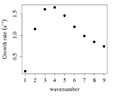
A careful treatment of the boundary conditions is important in the non-linear model (see main text) but we have found that the results of our linear model are not sensitive to the use of Dirichlet or Neumann boundary conditions. The growth rate of the fastest-growing radial eigenfunction for each wavenumber up to nine is shown in Fig. (8). The e-folding time (which is the reciprocal of the growth rate) for wavenumbers 3 or 4 is about 0.6 seconds (as in the numerical model: see section IV.2 of the main text).
Acknowledgements.
This work was supported by the Met Office Hadley Centre Climate Programme funded by BEIS and Defra. Thanks to Grae Worster and an anonymous referee of an earlier draft of this paper for pointing out the centrifugal instability of the boundary layer mentioned in section III.3. We acknowledge the contribution of the anonymous referees who helped to improve earlier drafts of this article. Thanks to Simon Hammett for the stop-motion filming, which facilitated an estimation of the velocity profile. Thanks to Mike Cullen, Paul Billant, Michael McIntyre, Mike Bell, Richard Wood, Adam Scaife, Eddy Carrol, Andy White, Nigel Wood, David Thomson, Philip Brohan and Matt Palmer for various helpful discussions, emails, advice and encouragement. ©British Crown Copyright 2020, Met Office This article may be downloaded for personal use only. Any other use requires prior permission of the author and AIP Publishing. This article appeared in American Journal of Physics 88, Issue 12, 1041 (2020) and may be found at https://doi.org/10.1119/10.0002438References
- (1) O. M. Phillips, “Shear-flow turbulence,” Annual Review of Fluid Mechanics, 1 (1), 245–264 (1969).
- (2) J. P. Kossin and W. H. Schubert, “Mesovortices in hurricane Isabel,” Bull. Amer. Meteor. Soc., pp. 151–153 (2004), doi:10.1175/BAMS-85-2-151.
- (3) A. Adriani, A. Mura, G. Orton, C. Hansen, F. Altieri, M. L. Moriconi, J. Rogers, G. Eichstädt, T. Momary, A. P. Ingersoll, G. Filacchione, G. Sindoni, F. Tabataba-Vakili, B. M. Dinelli, F. Fabiano, S. J. Bolton, J. E. P. Connerney, S. K. Atreya, J. I. Lunine, F. Tosi, A. Migliorini, D. Grassi, G. Piccioni, R. Noschese, A. Cicchetti, C. Plainaki, A. Olivieri, M. E. O’Neill, D. Turrini, S. Stefani, R. Sordini, and M. Amoroso, “Cluster of cyclones encircling Jupiter’s poles,” Nature, 555, 216–219 (2018), doi:10.1038/nature25491.
- (4) L. Illari, J. Marshall, P. Bannon, J. Botella, R. Clark, T. Haine, A. Kumar, S. Lee, K. J. Mackin, G. A. McKinley, M. Morgan, R. Najjar, T. Sikora, and A. Tandon, “ ”Weather in a Tank”: Exploiting laboratory experiments in the teaching of meteorology, oceanography, and climate,” Bull. Amer. Meteor. Soc., 90, 1619–1632 (2009), doi:/10.1175/2009BAMS2658.1.
- (5) J. Marshall and R. A. Plumb, Atmosphere, Ocean and Climate Dynamics: An Introductory Text (Elsevier Academic Press, 2007), 1 edition, Hardcover, ISBN: 9780125586917.
- (6) K. J. Mackin, N. Cook-Smith, L. Illari, J. Marshall, and P. Sadler, “The effectiveness of rotating tank experiments in teaching undergraduate courses in atmospheres, oceans, and climate sciences,” Journal of Geoscience Education, 60 (1), 67–82 (2012).
- (7) S. Shakerin, “Fluids demonstrations: Trailing vortices, plateau border, angle of repose, and flow instability,” The Physics Teacher, 56 (4), 248–252 (2018).
- (8) MIT, “General Circulation: Tank - Eddies,” (Accessed 2019), digital media. [Available online at http://weathertank.mit.edu/links/projects/general-circulation-an-introduction/general-circulation-tank-eddies.].
- (9) D. Fultz, R. R. Long, G. V. Owens, W. Bohan, R. Kaylor, and J. Weil, “Studies of thermal convection in a rotating cylinder with some applications for large-scale atmospheric motions,” Meteor. Monographs, pp. 1–104 (1959).
- (10) A. C. Barbosa Aguiar, P. L. Read, R. D. Wordsworth, T. Salter, and Y. H. Yamazaki, “A laboratory model of Saturn’s north polar hexagon,” Icarus, 206, 755–763 (2010).
- (11) J. Van de Konijnenberg, A. Nielsen, J. Rasmussen, and B. Stenum, “Shear flow instability in a rotating fluid,” J. Fluid Mech., 387, 177–204 (1999).
- (12) M. Nezlin and E. Snezhkin, Rossby vortices, spiral structures, solitons. Astrophysics and plasma physics in shallow water experiments (Springer, 1993), ISBN: 3540501150.
- (13) O. Reynolds, “An experimental investigation of the circumstances which determine whether the motion of water shall be direct or sinuous, and of the law of resistance in parallel channels,” Proc. Roy. Soc., 174, 935–982 (1883).
- (14) Grae Worster, “Kelvin Helmholtz,” (Accessed 2019), digital media. [Available online at https://www.youtube.com/watch?v=UbAfvcaYr00.].
- (15) D. H. Kelley and N. T. Ouellette, “Using particle tracking to measure flow instabilities in an undergraduate laboratory experiment,” American Journal of Physics, 79 (3), 267–273 (2011).
- (16) P. Vorobieff and R. E. Ecke, “Fluid instabilities and wakes in a soap-film tunnel,” American Journal of Physics, 67 (5), 394–399 (1999).
- (17) National Committee for Fluid Mechanics Films, “Vorticity,” (Accessed 2019), digital media. [Available online at http://web.mit.edu/hml/ncfmf.html.].
- (18) G. K. Batchelor, An introduction to fluid dynamics. (Cambridge University Press, 1967).
- (19) A. Tandon and J. Marshall, “Einstein’s tea leaves and pressure systems in the atmosphere,” The Physics Teacher, 48 (5), 292–295 (2010).
- (20) National Committee for Fluid Mechanics Films, “Secondary Flow,” (Accessed 2019), digital media. [Available online at http://web.mit.edu/hml/ncfmf.html.].
- (21) I. N. James, Introduction to Circulating Atmospheres (Cambridge University Press, 1994), 1 edition, Hardcover, ISBN: 0 521 41895 X.
- (22) M. Rabaud and Y. Couder, “A shear-flow instability in a circular geometry,” Journal of Fluid Mechanics, 136, 291–319 (1983).
- (23) D. Coles, “Transition in circular couette flow,” Journal of Fluid Mechanics, 21 (3), 385–425 (1965).
- (24) D. G. Andrews, An introduction to atmospheric physics (Cambridge University Press, 2010).
- (25) G. Vallis, Atmospheric and Oceanic Fluid Dynamics ( Cambridge University Press., 2006), 1 edition.