A simple and fast finite difference method for the integral fractional Laplacian of variable order
Abstract.
For the fractional Laplacian of variable order, an efficient and accurate numerical evaluation in multi-dimension is a challenge for the nature of a singular integral. We propose a simple and easy-to-implement finite difference scheme for the multi-dimensional variable-order fractional Laplacian defined by a hypersingular integral. We prove that the scheme is of second-order convergence and apply the developed finite difference scheme to solve various equations with the variable-order fractional Laplacian. We present a fast solver with quasi-linear complexity of the scheme for computing variable-order fractional Laplacian and corresponding PDEs. Several numerical examples demonstrate the accuracy and efficiency of our algorithm and verify our theory.
Key words and phrases:
Nonlocal Laplacian, Pseudo-differential operator, Approximation Properties, Convergence, Fast solver2010 Mathematics Subject Classification:
35B65, 65M70, 41A25, 26A332010 Mathematics Subject Classification:
65N06, 65N12, 65T50, 35R11, 26A331. Introduction
During the past few decades, fractional calculus has been extensively explored as a tool for developing more sophisticated but computationally tractable models. They can accurately describe complex physical phenomena, manifesting in long-range and nonlocal interactions, self-similar structures, sharp interfaces, and memory effects, which can not be adequately captured by their integer counterpart. One of the most important fractional calculus tools is the fractional Laplacian of the constant -th order, defined as an singular integral [5]
| (1.1) |
with a normalized constant , has been intensively investigated in the literature in the past two decades. In particular, various applications have been found for the nonlocal operators (1.1) such as fracture mechanics, image denoising, and phase field models in which jumps across lower-dimensional subsets and sharp transitions across interfaces (see [15, 18, 23, 42]).
1.1. Motivation for the variable-order model
The constant-order operator (1.1) may be less sufficient for the heterogeneous effect due to the spatial variability of complex medium. To account for heterogeneity, the variable-order operators depending on the spatial location variable have been alternatively proposed. In this work, we consider the following -th order fractional Laplacian
| (1.2) |
The variable-order extension variable order enables us to truly capture the non-smooth effects such as fractures by prescribing variable degree of smoothness across the scales. For example, the authors in [4] advocated the variable-order operator to perform regularization in image processing. They used large value of the order in the flat region and the smaller value in the neighborhood of edges. In [16, 7], the authors pointed out that the usage of the variable order is partially motivated from the theoretical study of galaxy rotation curves and the dark matter. Their study requires the field equation for the gravitational potential to become a variable-order fractional Poisson’s equation. Another example is from the groundwater flow. The authors in [25] justified that the super-diffusion depends on spatial variables due to the local variation of aquifer properties. We also refer the interested readers to other applications including biology [11], geophysics [28], spatial statistics [32] and so on.
When restricted to the bounded domain, equations with the fractional Laplacian of constant order as the leading operator usually have non-physical weak boundary singularity (boundary layer) unless boundary conditions are special. The boundary layer is often undesirable for the real world applications. As a remedy, the authors in [45] suggested to use the Caputo-type variable-order operator and analyzed a one-dimensional (1D) two-point boundary value problem. In Section 3.2, we use a variable-order fractional Laplacian requiring variable order along the boundary and observe in Example 3.3 that a full convergence order can be achieved on uniform meshes, which may suggest full regularity of solutions to such equations. This observation may lead to more practical fractional calculus in real applications.
1.2. Related definitions of variable-order fractional Laplacian
Changing directly the constant-order into the variable-order may increase not only the model capability but also the complexity in the computation. For example, one can use the variable-order function in place of in (1.2), which depends on both the spatial variable and the integration variable in the singular integral in the recent work [8, 29]. The wellposedness of corresponding fractional Poisson equations or other partial differential equations can be straightforwardly established from the variational formulation. However, the definition does not allow a simple Fourier transform of the fractional Laplacian as in the constant-order fractional Laplacian and Fourier-transformed based computational methods are not readily applicable.
The authors in [7] used the Fourier transform to extend the variable-order fractional Laplacian. However, the Fourier-type definition therein (see also Remark 2.2) is different from the one considered in this work. Here we prove that the singular integral type definition (1.2) can be rewritten via Fourier transforms but is different from the definition in [7]; see Theorem 2.1 for the details. One desirable feature of their definition is that the kernel is convolution-type but its explicit form is not available and have to be calculated through the forward and backward Fourier transforms.
Except for the above commonly used approaches to define the variable-order fractional Laplacian, one can also consider the spectral definition (see [44]) and harmonic-extension type definition (see [4]). For the spectral definition, the associated computation is straightforward when the eigen-values or eigen-functions are explicitly available. In this paper, we will not go through every definition but limit our attention into the singular-integral type (1.2).
1.3. Literature review and research gap
The close or explicit form of the -th order fractional Laplacian of functions seldom exists. In this work, we aim for an efficient numerical evaluation for the fractional Laplacian of variable order (1.2) with its applications in numerical solutions to nonlocal PDEs. In 1D case, we note that the authors in [46] showed the equivalence between the Fourier-type definition and two-sided Riemann-Liouville derivatives reformulation. Following upon their work, finite difference methods and fast solvers have been developed for the fractional Laplacian of coordinate-dependent type (see [30, 40]). However, to the best of our knowledge, we are not aware of any numerical results in 2D/3D in the literature due to the complexity of the operator discretization. Even if one can extend the finite difference scheme such as the popular Grunwald approximation to compute 1D variable-order fractional operators, the rigorous convergence analysis is not provided yet. The current research aims to fill this computational and theoretical gap.
For the constant-order fractional Laplacian, some progress has been made and extensive numerical methods have been developed among the computational mathematics community particularly during the past around five years. Finite or boundary element methods are developed in the context of the boundary integral equations, and they can be straightforwardly extended to solve the integral equations involving the volume integral (see [1]). However, it is extremely difficult to implement the finite element methods (FEM) particularly in 3D as it entails complicated numerical quadrature for the double integrals [12]. To avoid the expensive computation of the double integrals, meshless methods or collocation methods have been developed. For special domains such as a disk, the accurate and efficient spectral method using the eigen-functions was proposed in [43] and [19]. For a general domain, radial basis functions (RBF) methods using the standard Gaussian functions [6] and other generalized multi-quadratic functions have been developed. However, RBF methods suffer from the notorious ill-condition issue which makes it harder for solving the large-scale size problem.
For the large-scale computation and easy implementation in multi-dimensions for fractional Laplacian of constant order, finite difference methods or collocation methods have been proposed recently. Using the singularity subtraction technique, the authors in [27] proposed a simple solver via the Taylor expansion under the high-regularity assumption that the target function but the stability of the finite difference scheme is unknown. The authors in [9] converted the fractional Laplacian with the strong singularity into the one with the weak singularity through the integration by parts, and then constructed a quadrature-based finite difference approximation. However, the stability estimates were not provided and it is not clear if the associated finite difference scheme is stable when applied to the numerical solution of PDEs involving the fractional Laplacian operator. The authors in [2] presented the collocation method based on the sinc basis functions and rigorous analysis of the method was later provided in [3]. Nonetheless, the analysis therein relies on the properties of Fourier transform and cannot be directly extended to the problem considered in this work.
We remark that the Fourier transform of fractional Laplacian of constant-order allows designs of various and efficient numerical methods. However, this is not the case for the variable-order fractional Laplacian as the semi-group and symmetry properties cannot extend, and the explicit and elementary representation of the Fourier transform of variable order does not exist. Without these properties, straightforward extensions of previous working numerical methods are highly nontrivial including various discretization methods such as spectral methods in [38, 37], the fast finite element implementation [34], Dunford-Taylor reformulation based finite element methods and spectral methods and so on.
In [20] we establish an easy-to-implement and efficient finite difference method based on the generating functions approximation theory. The computation of the coefficients or weights in finite difference approximation can be efficiently calculated through the fast discrete Fourier transform and a fast solver is implemented for the structured resulting linear systems. Along this line of research, we aim to extend the idea of simple finite difference discretization in [20] to the variable-order context, and propose an efficient solver for the resulting unstructured matrix induced by the non-convolution kernel in the variable-order operator (1.2).
1.4. Contributions and outline of this work
The significance and novelty of the paper is that it is the first work addressing a fast and accurate finite difference approximation for the numerical evaluation of the multi-dimensional fractional Laplacian of variable order (1.2). Our approximation is robust and stable in the sense that we can get a second-order approximation even for the nonsmooth piecewise variable-order function (see Tables 1, 2 and 3).
The approximation is derived from the discrete Fourier transform. Although the explicit form of the Fourier transform for the variable-order case does not exist, we find that it can be defined through the Fourier transform as in the constant-order case. Such equivalence allows us to discretize the singular operator in the frequency space which avoids the complicated quadrature.
Compared to the constant-order counterpart, the variable-order definition in multi-dimensions uses the non-convolution kernel and thus the corresponding discrete counterpart becomes non-Toeplitz, which brings up the extra computational difficulty regarding the efficient solver part. Nonetheless, by the Fourier transformation and the low-rank approximation of the Fourier symbol (see Lemma 2.4), we are able to overcome the difficulty and construct a fast solver based on the observation that the unstructured resulting matrix can be approximately decomposed into the linear combination of the structured matrices.
Several numerical results are demonstrated to show the accuracy and efficiency of the proposed scheme. Numerically, we find that the appropriately selected variable-order model can avoid the non-physical boundary singularity as in the constant-order model.
In a nutshell, the main contributions of this work are described as follows.
-
•
We establish the equivalence and provide its proof between Fourier-type definition and singular-integral form.
-
•
We derive a second-order finite difference approximation for the variable-order fractional Laplacian in multi-dimensions and present a rigorous convergence analysis.
-
•
We provide a fast solver with quasi-linear complexity to efficiently compute the variable-order operator and related PDEs.
-
•
We apply the developed finite difference discretization to solve various fractional PDEs with variable-order fractional Laplacian and carry out the extensive numerical experiments to show the accuracy and efficiency of our theory and algorithm.
We organize this paper as follows. In Section 2, we present a fractional finite difference approximation based on the equivalence between the Fourier-type definition and singular integral form. Moreover, we describe its implementation with a quasilinear fast solver, and show the accuracy and robustness of our approximation. In Section 3, we apply the discrete approximation to the numerical solution for the nonlocal elliptic PDEs. We carry out the extensive numerical experiments and demonstrate the accuracy and efficiency of our scheme. We put the proofs of the theoretical results in Section 4 for the interested readers, including the second-order approximation and the convergence analysis for the finite difference method in 1D case. Finally, we conclude this work in Section 5.
2. A second-order finite difference approximation
In Subsection 2.1, we establish the equivalence for fractional-order Laplacian between singular integral form and the Fourier transform. Such equivalent characterization provides us different perspectives and a starting point to design an efficient numerical method, the finite difference method via the semi-discrete Fourier transform which will be described in Subsection 2.2. We describe the implementation for the calculation of the coefficients or weights associated with the approximation in Subsection 2.3 and the fast solver in Subsection 2.4. Finally we present a numerical example in Subsection 2.5.
2.1. Variable-order fractional Laplacian defined via Fourier transform
In our discussion, we assume that the variable-order function in the definition (1.2) is continuous and bounded, that is , and
| (2.1) |
The Fourier transform and its inverse are defined respectively as follows
| (2.2) |
and
| (2.3) |
where is the complex symbol . Following the argument in the constant case as in [5], we show that the equivalence of two definitions still holds in the variable-order context.
Theorem 2.1 (Equivalence of the definitions).
Let , which is the space of bounded and twice continuously differentiable functions. The -th variable-order fractional Laplacian is equivalent to the one defined in the Fourier transform, i.e.,
| (2.4) |
when both sides of the equality (2.4) are well-defined.
Remark 2.2.
In [7], the authors proposed the Fourier-type fractional Laplacian as follows:
| (2.5) |
It is clear that the two Fourier-type definitions are different since the inverse of the Fourier transform of kernel function is the univariate function in variable which is not equal to the function . Note that the definition (2.5) leads to the convolution type operator while the definition (1.1) is the type of non-convolution.
The equivalence of the definitions inspires us to discretize the operator in the Fourier or frequency spaces rather than the direct discretization in the physical space using the complicated finite difference-quadrature.
2.2. A second-order finite difference approximation
Denote as the spatial stepsize of the grids. Let be the set of infinite grids, i.e.,
| (2.6) |
Throughout the paper, the summation index is multi-index, so is the index .
For a function , define the semi-discrete Fourier transform as
| (2.7) |
Denote the parameterized domain . Then we have the discrete Fourier inversion formula
| (2.8) |
For a continuous function , let for . Inspired by the idea for 1D in [21] and our previous work [20] for multi-dimensional cases, we propose the discrete variable-order Laplacian operator as follows:
| (2.9) |
with
| (2.10) |
Introduce the following spectral Barron space (see [10, 26])
| (2.11) |
and the induced norm . It is clear that for .
For any grid function on , define the discrete maximum norm as
We state the main theoretical result in this work.
Theorem 2.3 (Approximation properties).
We postpone the proof of second-order approximation properties and put it in the section 4.
2.3. Implementation
In the practical computation, we want to numerically evaluate the operator at the grid points, that is, . Thus, we have
| (2.13) | |||||
where the weights
| (2.14) |
Making a change of variable leads to
| (2.15) |
In the practical computation, for each fixed grid point , we need to compute the coefficients for for (Here and denotes the number of grid points in direction. For the sake of simplicity, let us assume they all equals to ).
To alleviate the burden of tedious notations, we drop the dependence on the variable and abbreviate it as without the confusion.
In 1D, the analytical expression of the above integrals can be derived. In fact, recall the formula [17, Page 399, 3.631.9]
| (2.16) |
Here denotes the Beta function. Take , and make a change of variable . Then the formula (2.16) reduces to
| (2.17) | |||||
Due to the symmetry of the integrand, the coefficients (2.15) can be reduced to
| (2.18) | |||||
In multi-dimension cases, since the explicit formula is difficult to derive, we will use the standard numerical integration to compute the integrals. Specifically, take an integer number (here denote the number of grid points in direction) and step-size . Denote . Applying the trapezoidal rule, we have
| (2.19) | |||||
With the expression above we can use Matlab built-in function ‘ifftn’ to compute the coefficients for efficiently with the computational cost .
2.4. Fast computation of the discrete variable-order Laplacian
In this subsection we present a fast solver for the numerical evaluation of the fractional Laplacian. In general, we are interested in the numerical evaluation of the target function restricted in the bounded computational domain . Suppose that is a square (or a rectangular domain if we take a nonisotropic different mesh size in each spatial direction in the last subsection). If not, we can embed the general bounded domain into a larger square (or rectangular) domain , consider the evaluation on the domain instead and do the restriction in the domain . The following lemma is a key to develop a fast algorithm.
Lemma 2.4.
For any tolerance , there exists integer such that
| (2.20) |
where ’s are Chebyshev points in the interval and ’s are associated Lagrange polynomials.
Proof.
Consider the univariant function for and . By the Lagrange interpolation associated with the Chebyshev points (see [22]), we have
| (2.21) |
Here . Then replace with , and the exponent by , respectively, which immediately leads to the desired result. ∎
As direct consequence of the above lemma, we can use the superposition principle, the linear combination of the constant-order discrete fractional operators to approximate the variable-order fractional Laplacian to achieve a fast computation. That is
| (2.22) |
Based on the above discussion, we describe our algorithm for the numerical evaluation as follows:
Algorithm 2.5.
For the fractional Laplacian of the variable order, we have the following computation.
-
•
Step 1, generate the Chebyshev points , and evaluate Lagrange polynomials for and with for .
-
•
Step 2, for each fixed constant-order , compute for , and then multiply the diagonal matrix .
-
•
Step 3, add them together over .
Note that, in Step 2, we refer the readers to [20] for implementation details.
2.5. Numerical experiments
In the following example, we take the Gaussian function as our test function to illustrate the accuracy of the theoretical result.
Example 2.6 (Approximations of variable-order fractional Laplacian in multi-dimensions).
Consider the Gaussian function with a truncated computational domain , where is for the dimension and .
In this experiment, the variable-order Laplacian of the Gaussian function is given as (see the Appendix for the derivation)
| (2.23) |
The error is measured as , and the convergence order is estimated by .
Note that the function is smooth and satisfies the regularity requirement in Theorem 2.3. Here we examine the effect of the variable order on the accuracy of the finite difference approximation. Tables 1-3 show the errors and convergence orders for different in 1D/2D/3D, respectively. Three different with different range and smoothness are tested. From the tables, we observe that our approximation is of second order, which agrees with the predicted convergence order in Theorem 2.3. In particular, the approximation is very robust in the sense that we are still able to get the second-order convergence even for the non-smooth piece-wise function .
| Order | Order | Order | ||||
|---|---|---|---|---|---|---|
| 1/4 | 1.17e-02 | * | 2.25e-02 | * | 1.68e-02 | * |
| 1/8 | 2.93e-03 | 1.99 | 5.69e-03 | 1.98 | 4.23e-03 | 1.99 |
| 1/16 | 7.35e-04 | 2.00 | 1.44e-03 | 2.00 | 1.06e-03 | 2.00 |
| 1/32 | 1.84e-04 | 2.00 | 3.61e-04 | 2.00 | 2.65e-04 | 2.00 |
| 1/64 | 4.61e-05 | 2.00 | 9.03e-05 | 2.00 | 6.62e-05 | 2.00 |
| Order | Order | Order | ||||
|---|---|---|---|---|---|---|
| 1/4 | 2.06e-02 | * | 2.68e-02 | * | 3.05e-02 | * |
| 1/8 | 1.33e-02 | 1.99 | 5.19e-03 | 1.99 | 7.69e-03 | 1.99 |
| 1/16 | 3.32e-03 | 1.99 | 1.31e-03 | 1.99 | 1.93e-03 | 1.99 |
| 1/32 | 8.28e-04 | 2.00 | 3.37e-04 | 1.97 | 4.90e-04 | 1.98 |
| Order | Order | Order | ||||
|---|---|---|---|---|---|---|
| 3.98e-01 | * | 3.98e-01 | * | 5.83e-01 | * | |
| 1.10e-01 | 1.86 | 1.43e-01 | 1.48 | 1.64e-01 | 1.83 | |
| 2.81e-02 | 1.96 | 3.97e-02 | 1.85 | 4.23e-02 | 1.96 | |
3. Application on fractional PDEs
3.1. Finite difference scheme for the elliptic equations
In this section, we will apply the proposed discrete operator into solving the elliptic equations and parabolic equations with the variable-order fractional Laplacian. For the parabolic equations, after the semi-discretization in temporal direction, they are reduced to the elliptic one at the each time step. Thus we only discuss the elliptic case as below:
| (3.1) | |||
| (3.2) |
where the reaction coefficient is non-negative, the right-hand-side function is given, is the standard bounded domain with the sufficiently smooth boundary and is the complement of in .
Remark 3.1.
Regarding the mathematical theory related to the variable-order fractional Laplacian, the authors in [14] showed that the kernel admits the lower bounded Dirichlet form. Later the authors in [13] set up the elliptic and the parabolic Dirichlet problem for the linear nonlocal operators which cover the special case as in this work. The paper formulated the problem in the classical framework of Hilbert spaces and proved unique solvability using standard techniques like the Fredholm alternative. In [35], the author investigated the Hölder regularity of the elliptic equations with a variable-order fractional Laplace operator.
Consider Equation (Eq.) (3.1) at the grid points and we obtain
| (3.3) |
Replacing the fractional Laplacian by the difference operator defined in Eq. (2.9), Eq. (3.3) becomes
| (3.4) |
with the truncation error depending on the solution . By Theorem 2.3, we assume with a positive constant , such that there exists a constant satisfying
| (3.5) |
Omitting in Eq. (3.4) and denoting by the numerical approximation of , and (the short notation will be frequently used throughout the following without the confusion), and , we get the finite difference scheme
| (3.6) | |||
| (3.7) |
Theorem 3.2 (Stability and Convergence).
For any , the finite difference scheme (3.6)-(3.7) is uniquely solvable and stable with respect to the right hand side in the following sense
| (3.8) |
Moreover, let be the solution of Eqs. (3.1)-(3.2) and be the numerical solution of the difference scheme (3.6)-(3.7). Assuming that the solution with , it holds that
| (3.9) |
3.2. Numerical Experiments
In this subsection, several numerical examples are presented to show the efficiency and accuracy of the schemes. We first apply the proposed finite difference scheme to solve the elliptic equation in Example 3.3 and the time-dependent problem in Example 3.4, respectively. To show the wide application of finite difference method, the finite difference scheme is applied to solve Allen-Cahn equation in Example 3.5. In addition, we consider the coexistence of anomalous diffusion problem in Example 3.6. In the last Example 3.7, we turn to the time-dependent problem in 3D.
Throughout the examples, the low-rank approximation terms is taken as to compute the Chebyshev points and the quadrature number is taken as to compute the coefficients in Step 2 so that the accuracy of numerical solution will not be polluted. The tolerance of the BiCGSTAB (see [39]) method is set as and the initial guess is fixed as zero in our simulations. All the simulations are performed in MATLAB 2021b on a 64-bit Ubuntu with Intel Xeon(R) Gold 6240 CPU processor at 2.60 GHz and 126 GB of RAM.
Example 3.3 (Finite difference scheme for variable-order fractional elliptic equations).
Consider the elliptical equations with variable-order fractional Laplacian on . Case 1: and the exact solution is set as ; Case 2: , the exact solution is unknown and the right-hand data is .
In Case 1, we take . Since the right hand side is unknown, we need to compute it with very fine step-size which is set as with small . In Table 4, the errors and convergence orders are listed with different . Here, the error is measured as . Furthermore, from Table 4, we can observe that the convergence order of our scheme is of second order.
Next we consider Case 2, where and the exact solution is unknown. Table 5 shows the errors and convergence orders with different . Here, the error is measured as . From the table, we observe that the convergence order is less than second order and is around , where .
In particular, if is a non-smooth piece-wise function, Table 4 shows that our scheme (3.6)-(3.7) still maintains second-order convergence when the exact solution is smooth enough. But the convergence order reduces to when the right-side data and the exact solution is unknown; see Table 5. The reason for the reduced convergence is that the solution may have the interior singularity inherited from the variable-order function.
To recover the second-order convergence rate, we take satisfying on and in . Figure 1 shows the profile of the function . From Table 6, we observe that the appropriately selected variable-order function enables us to recover the second-order convergence. We remark that for the case 1 corresponding to the first column results in Table 6, we further test the smaller case and and the convergence orders are 1.69 and 3.02, respectively. Thus the average order is around 2. For the case 2 in the second column, we also take smaller stepsize and the convergence order is 2.1. This implies that setting the variable-order can change the regularity of the solution and avoid the non-physical boundary singularity which reduces the convergence order as in Table 5.
| Order | Order | Order | ||||
|---|---|---|---|---|---|---|
| 1/4 | 2.26e-02 | * | 1.86e-02 | * | 1.15e-02 | * |
| 1/8 | 5.61e-03 | 2.01 | 4.46e-03 | 2.06 | 4.01e-03 | 1.52 |
| 1/16 | 1.40e-03 | 2.00 | 1.11e-03 | 2.01 | 1.04e-03 | 1.94 |
| 1/32 | 3.51e-04 | 2.00 | 2.78e-04 | 1.99 | 2.63e-04 | 1.99 |
| Order | Order | Order | ||||
|---|---|---|---|---|---|---|
| 1/8 | 6.88e-03 | * | 3.40e-02 | * | 1.28e-02 | * |
| 1/16 | 4.33e-03 | 0.67 | 2.53e-02 | 0.43 | 6.20e-03 | 1.05 |
| 1/32 | 2.68e-03 | 0.69 | 1.95e-02 | 0.38 | 3.68e-03 | 0.75 |
| 1/64 | 1.63e-03 | 0.71 | 1.56e-02 | 0.32 | 1.96e-03 | 0.91 |
| Order | Order | Order | Order | |||||
|---|---|---|---|---|---|---|---|---|
| 1/8 | 7.38e-03 | * | 2.25e-02 | * | 1.19e-03 | * | 2.65e-03 | * |
| 1/16 | 2.74e-03 | 1.43 | 7.48e-03 | 1.59 | 2.90e-04 | 2.03 | 6.76e-04 | 1.97 |
| 1/32 | 9.36e-04 | 1.55 | 2.26e-03 | 1.73 | 7.14e-05 | 2.02 | 1.70e-04 | 1.99 |
| 1/64 | 2.99e-04 | 1.65 | 6.46e-04 | 1.81 | 1.76e-05 | 2.02 | 4.25e-05 | 2.00 |

Example 3.4 (Time-dependent problem).
Consider the initial-boundary value problem with variable-order fractional Laplacian
| (3.10) | |||
| (3.11) |
with the initial condition .
In this example, we test the convergence order of spatial direction at the final time , where is time step-size. Since the solution decays to zero, we truncate the finite domain in space, as our computational domain. For time discretization we use Crank-Nicolson scheme. Since the exact solution is unknown, the error is measured as .
Table 7 shows the errors and convergence orders in for different , from which the second-order convergence can be observed. This is in agreement with the second-order approximation of our theoretic prediction.
| error | Order | error | Order | ||
|---|---|---|---|---|---|
| 1/2 | 1/2 | 1.34e-02 | * | 2.36e-02 | * |
| 1/4 | 1/4 | 3.07e-03 | 2.12 | 4.54e-03 | 2.38 |
| 1/8 | 1/8 | 7.85e-04 | 1.97 | 1.12e-03 | 2.02 |
| 1/16 | 1/16 | 1.99e-04 | 1.98 | 2.82e-04 | 1.99 |
Example 3.5 (Allen-Cahn equation with the variable-order fractional Laplacian).
Consider the following nonlocal Allen-Cahn equation which is used in modeling phase field problems arising in materials science and fluid dynamics
| (3.12) | |||
| (3.13) |
The computational domain is , and is the phase field function. The initial condition is chosen as
where the constant describes the diffuse interface width, the function and . Here, we apply our method to study the benchmark problem coalescence of two ”kissing” bubbles in the phase field models. Letting , we can reformulate the problem (3.12) as an equation of with the extended homogeneous boundary conditions. Three-level linearized finite-difference scheme (see [41]) is used in the simulation.
In the simulations, we take the mesh size and the time step . Figure 2 shows the dynamics of the two bubbles described by the variable-order fractional Allen-Cahn equations with . Initially, the two bubbles are centered at points and , respectively. When , the two bubbles first coalesce into one bubble, and then the newly formed bubble shrinks and finally is absorbed by the fluid (see the middle column in Figure 2). However, the smaller the value of the variable-order becomes, the slower coalescence and disappearing of the two bubbles get (see the right column in Figure 2). By contrast, if , the two bubbles do not merge, and they eventually vanish at the different time due to the inhomogeneous distribution of the variable-order function on (see the left column in Figure 2). From Figure 3, we can see the two single bubbles will be absorbed by the fluid. Figure 4 shows the profiles of different on tested in the simulation.


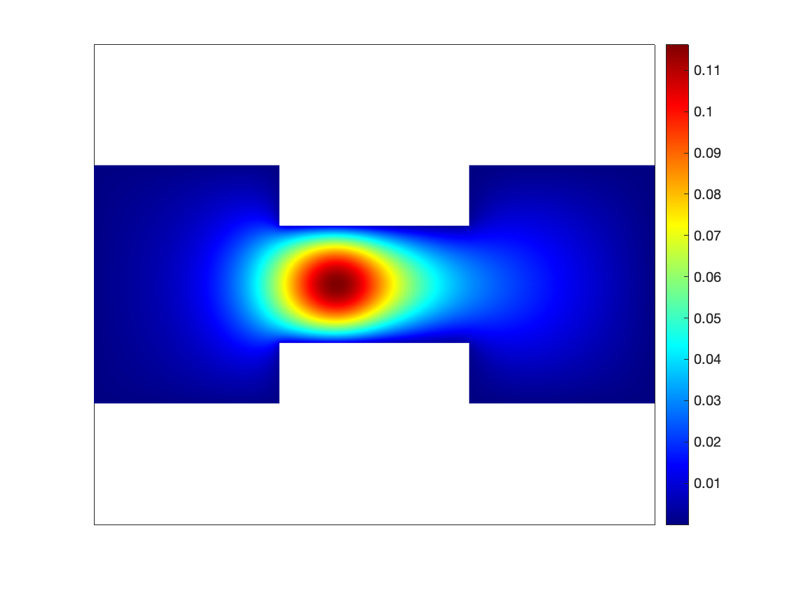
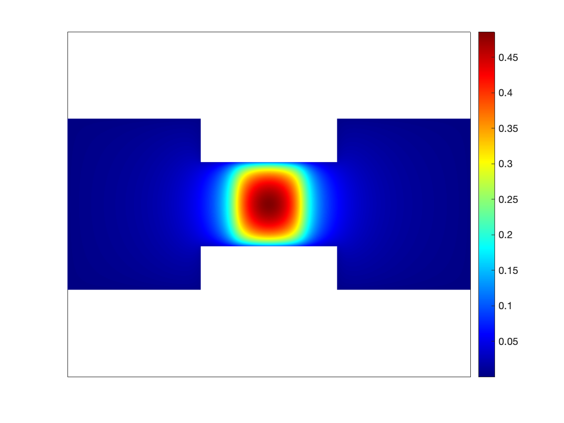
Example 3.6 (Coexistence of anomalous diffusion problem [24]).
Consider the coexistence of anomalous diffusion problem:
In the simulation, we extend the irregular domain (Figure 5) into a large rectangular one such that . Then, we can transform the original problems into the one defined on rectangular domain [20].
Figure 6 shows the dynamics of the coexistence of anomalous diffusion equation with different . Here, we set the rectangular domain , the diffusion coefficient and initial condition . For time discretization we use Crank-Nicolson scheme with and . We find that the smaller the order , the slower the rate of diffusion (see the left and middle columns in Figure 6). However, when the order exhibits significantly heterogeneous at both ends of the center point, the large power side represents faster diffusion rate than the other side and even weaken it (see Figure 6 for the right column).


Example 3.7 (Application to the time-dependent problem in 3D).
Consider the 3D time-dependent variable-order fractional diffusion problem [27]:
Here, the right hand side is set as with and the initial condition
with . We use the second-order finite difference approximation for spatial discretization and a Crank-Nicolson method for the temporal discretization, respectively. To demonstrate the efficiency of our methods, we present the CPU time of solving the 3D linear system of equations by the BiCGSTAB method and corresponding BiCGSTAB iterations for a single time step with different in Table 8. For convenience, at the bottom of Table 8 we give an estimate of the asymptotic decay rate of the error as increases, which is achieved by a least-squares fit of the log-error to log-. It shows that for fixed and , the time gets longer for larger , because the stiffness matrix from larger has bigger conditional number and it will affect the BiCGSTAB iterations. Furthermore, the corresponding timing results are plotted in Figure 7.
| 1/32 | 4.78e+01 | 13 | 5.33e+01 | 38 | 7.78e+01 | 94 | 6.31e-01 | 61 | |
| 1/64 | 9.94e+01 | 13 | 1.86e+02 | 47 | 4.58e+02 | 158 | 6.82e+00 | 86 | |
| 1/128 | 6.23e+02 | 14 | 1.70e+03 | 55 | 6.67e+03 | 243 | 8.70e+01 | 116 | |
| 1/256 | 5.20e+03 | 14 | 1.77e+04 | 63 | 8.05e+04 | 330 | 1.03e+03 | 153 | |
| Rate | 2.26 | * | 2.79 | * | 3.35 | * | 3.52 | * | |

4. Proofs
In this section, we present the proofs of conclusions in Sections 2 and 3.
4.1. Proof of Theorem 2.1
Proof.
By the definition of variable-order fractional Laplacian (1.2), we can rewrite it as follows
| (4.1) |
It remains to show that the definition of variable-order fractional Laplacian via Fourier transform (2.4) can be also written in this form.
Recalling the identity (e.g., see [5])
| (4.2) |
we have
| (4.3) | |||||
Taking the inverse Fourier transform on both sides leads to
| (4.4) | |||||
where we have used Fubini’s theorem for the second equal sign. This completes the proof. ∎
4.2. Proof of Theorem 2.3
In this subsection, we present the proof for the second-order approximation in Theorem 2.3. The semi-discrete Fourier transform is closely connected with the continuous Fourier transform. The following lemma is needed in our proof.
Lemma 4.1 (Poisson summation formula).
Let be such that its Fourier transform is also absolutely integrable, and satisfies the two estimates and for positive . Then we have the identity
Proof.
Recall the Poisson summation formula (e.g., see Chapter 4 in [31].)
| (4.5) |
The convergence of the sums is in . If satisfies the two estimates and for positive , then the two sums above are absolutely convergent and their limiting functions are continuous. Therefore the above identity holds pointwise. By the scaling property of the Fourier transform, we have
By the definition of the semi-discrete transform (2.7), we can obtain the desired result. ∎
The Poisson summation formula is essential to prove the convergence of our discrete approximation. By Taylor expansion, it is not hard to prove the following estimates for in (2.10):
| (4.6) | |||
| (4.7) |
for and sufficiently small . Here and throughout the following, is a constant independent of the step-size and the function but may change from line to line.
Proof.
For with , it is clear that and the grid function is well defined. We use the semi-Fourier analysis technique to estimate the convergence of the discrete operator. For ,
| (4.8) | |||||
where each integral is defined below
We estimate each term in (4.8). For the first item , we need to estimate the difference in the integrand. Noting the assumption and by the Poisson summation formula, we have
Plugging in and using the equivalence (4.7), we have
For the second term similarly we have
For the third term, we have
Combining the estimates of ’s together leads to the desired result. ∎
4.3. Proof of Theorem 3.2
Here we analyze the stability and convergence of the finite difference scheme for the fractional elliptic equation on the unit interval . For simplicity, we assume that the variable coefficient .
The stiffness matrix associated with the discrete fractional Laplacian operator with the variable-order is
We use the maximum value principle to analyze the stability of the scheme. To this end, we need to examine the properties of the coefficients in the discrete fractional Laplacian defined in (2.13).
The properties of the coefficients are stated in the following lemma.
Lemma 4.2.
For the coefficients defined in (2.15), we have the following properties.
-
(1)
For fixed , and for .
-
(2)
The summation of the coefficients equal to zero, that is .
-
(3)
We have the estimates
(4.9)
Proof.
For proof, the interested readers may refer to [36]. ∎
Lemma 4.3.
Let be a monotone matrix of order and is a normalized vector, such that for some positive scalar . Then we have
With the above lemma, we are ready to present the stability and convergence of the difference scheme (3.6)-(3.7).
Proof.
Combining with the consistent error described in Theorem 2.3, we can readily obtain the convergence.
5. Conclusion
In this work, we considered the numerical evaluation of the variable-order fractional Laplacian particularly in 1D, 2D and 3D. Based on the generating function theory on the central finite difference schemes, we derived an efficient finite difference method for the fractional Laplacian of the variable-order. We developed a fast solver with the quasi-optimal complexity for the computation of discrete operators and numerical solution for the relevant nonlocal PDEs with variable-order fractional Laplacian. We discussed the implementation of the proposed scheme and reported numerical results to illustrate the accuracy and efficiency of our method and verify our theoretical predictions. In this work, we only provide the stability and convergence analysis in 1D and we hope to address the analysis in 2D and 3D in our future work.
Acknowledgement
Z. Hao would like to thank Professor Yanzhi Zhang from Missouri University of Science and Technology for stimulating discussions for this work, and the support of a start-up grant from Southeast University in China. R. Du would like to thank the support by the Natural Science Foundation of Jiangsu Province (Grant No. BK20221450).
References
- [1] M. Ainsworth and C. Glusa, Aspects of an adaptive finite element method for the fractional Laplacian: a priori and a posteriori error estimates, efficient implementation and multigrid solver, Comput. Methods Appl. Mech. Engrg., 327 (2017), pp. 4–35.
- [2] H. Antil, P. Dondl, and L. Striet, Approximation of integral fractional Laplacian and fractional PDEs via sinc-basis, SIAM J. Sci. Comput., 43 (2021), pp. A2897–A2922.
- [3] H. Antil, P. W. Dondl, and L. Striet, Analysis of a sinc-galerkin method for the fractional laplacian, SIAM J. Numer. Anal., 61 (2023), pp. 2967–2993.
- [4] H. Antil and C. N. Rautenberg, Sobolev spaces with non-Muckenhoupt weights, fractional elliptic operators, and applications, SIAM J. Math. Anal., 51 (2019), pp. 2479–2503.
- [5] C. Bucur and E. Valdinoci, Nonlocal diffusion and applications, Springer, 2016.
- [6] J. Burkardt, Y. Wu, and Y. Zhang, A unified meshfree pseudospectral method for solving both classical and fractional PDEs, SIAM J. Sci. Comput., 43 (2021), pp. A1389–A1411.
- [7] E. Darve, M. D’Elia, R. Garrappa, A. Giusti, and N. L. Rubio, On the fractional Laplacian of variable order, Fract. Calc. Appl. Anal., 25 (2022), pp. 15–28.
- [8] M. D’Elia and C. Glusa, A fractional model for anomalous diffusion with increased variability: Analysis, algorithms and applications to interface problems, Numer. Methods Partial Differential Equations, 38 (2022), pp. 2084–2103.
- [9] S. Duo and Y. Zhang, Accurate numerical methods for two and three dimensional integral fractional Laplacian with applications, Comput. Methods Appl. Mech. Engrg., 355 (2019), pp. 639–662.
- [10] W. E, C. Ma, and L. Wu, The Barron space and the flow-induced function spaces for neural network models, Constr. Approx., 55 (2022), pp. 369–406.
- [11] M. E. Farquhar, T. J. Moroney, Q. Yang, I. W. Turner, and K. Burrage, Computational modelling of cardiac ischaemia using a variable-order fractional Laplacian, arXiv preprint arXiv:1809.07936, (2018).
- [12] B. Feist and M. Bebendorf, Quadrature rules for singular double integrals in 3D, arXiv:2208.05714, (2022).
- [13] M. Felsinger, M. Kassmann, and P. Voigt, The Dirichlet problem for nonlocal operators, Math. Z., 279 (2015), pp. 779–809.
- [14] M. Fukushima and T. Uemura, Jump-type Hunt processes generated by lower bounded semi-Dirichlet forms, Ann. Probab., 40 (2012), pp. 858–889.
- [15] P. Gatto and J. S. Hesthaven, Numerical approximation of the fractional Laplacian via -finite elements, with an application to image denoising, J. Sci. Comput., 65 (2015), pp. 249–270.
- [16] A. Giusti, R. Garrappa, and G. Vachon, On the Kuzmin model in fractional Newtonian gravity, Eur. Phys. J. Plus, 135 (2020).
- [17] I. S. Gradshteyn and I. M. Ryzhik, Table of integrals, series, and products, Academic press, 2014.
- [18] M. Gunzburger, N. Jiang, and F. Xu, Analysis and approximation of a fractional Laplacian-based closure model for turbulent flows and its connection to Richardson pair dispersion, Comput. Math. Appl., 75 (2018), pp. 1973–2001.
- [19] Z. Hao, H. Li, Z. Zhang, and Z. Zhang, Sharp error estimates of a spectral Galerkin method for a diffusion-reaction equation with integral fractional Laplacian on a disk, Math. Comp., 90 (2021), pp. 2107–2135.
- [20] Z. Hao, Z. Zhang, and R. Du, Fractional centered difference scheme for high-dimensional integral fractional Laplacian, J. Comput. Phys., 424 (2021), p. 109851.
- [21] Y. Huang and A. Oberman, Finite difference methods for fractional laplacians, arXiv preprint arXiv:1611.00164, (2016).
- [22] Y. Klokov and A. Shkerstena, Error estimates for lagrange-chebyshev interpolation formulae, USSR Computational Mathematics and Mathematical Physics, 27 (1987), pp. 93–95.
- [23] N. Laskin, Fractional quantum mechanics and Lévy path integrals, Phys. Lett. A, 268 (2000), pp. 298–305.
- [24] E. Lenzi, H. Ribeiro, A. Tateishi, R. Zola, and L. Evangelista, Anomalous diffusion and transport in heterogeneous systems separated by a membrane, Proceedings of the Royal Society A: Mathematical, Physical and Engineering Sciences, 472 (2016), p. 20160502.
- [25] X. Liu, H. Sun, Y. Zhang, C. Zheng, and Z. Yu, Simulating multi-dimensional anomalous diffusion in nonstationary media using variable-order vector fractional-derivative models with kansa solver, Advances in Water Resources, 133 (2019), p. 103423.
- [26] Y. Meng and P. Ming, A new function space from Barron class and application to neural network approximation, Commun. Comput. Phys., 32 (2022), pp. 1361–1400.
- [27] V. Minden and L. Ying, A simple solver for the fractional Laplacian in multiple dimensions, SIAM J. Sci. Comput., 42 (2020), pp. A878–A900.
- [28] X. Mu, J. Huang, L. Wen, and S. Zhuang, Modeling viscoacoustic wave propagation using a new spatial variable-order fractional laplacian wave equation, Geophysics, 86 (2021), p. T487–T507.
- [29] J. Ok, Local Hölder regularity for nonlocal equations with variable powers, Calc. Var. Partial Differential Equations, 62 (2023), pp. 1–31.
- [30] H.-K. Pang and H.-W. Sun, A fast algorithm for the variable-order spatial fractional advection-diffusion equation, J. Sci. Comput., 87 (2021), pp. 15–28.
- [31] M. A. Pinsky, Introduction to Fourier analysis and wavelets, vol. 102 of Graduate Studies in Mathematics, American Mathematical Society, 2009.
- [32] M. D. Ruiz-Medina, V. V. Anh, and J. M. Angulo, Fractional generalized random fields of variable order, Stochastic Analysis and Applications, 22 (2004), pp. 775–799.
- [33] C. Sheng, J. Shen, T. Tang, L.-L. Wang, and H. Yuan, Fast Fourier-like mapped Chebyshev spectral-Galerkin methods for PDEs with integral fractional Laplacian in unbounded domains, SIAM J. Numer. Anal., 58 (2020), pp. 2435–2464.
- [34] C. Sheng, L. Wang, H. C. Chen, and H. Li, Fast implementation of FEM for integral fractional Laplacian on rectangular meshes, Commun. Comput. Phys., (2023).
- [35] L. Silvestre, Hölder estimates for solutions of integro-differential equations like the fractional Laplace, Indiana Univ. Math. J., 55 (2006), pp. 1155–1174.
- [36] Z.-z. Sun and G.-h. Gao, Fractional differential equations–finite difference methods, De Gruyter, Berlin Science Press, Beijing, 2020.
- [37] T. Tang, L.-L. Wang, H. Yuan, and T. Zhou, Rational spectral methods for PDEs involving fractional Laplacian in unbounded domains, SIAM J. Sci. Comput., 42 (2020), pp. A585–A611.
- [38] T. Tang, H. Yuan, and T. Zhou, Hermite spectral collocation methods for fractional PDEs in unbounded domains, Commun. Comput. Phys., 24 (2018), pp. 1143–1168.
- [39] H. A. van der Vorst, Bi-CGSTAB: A fast and smoothly converging variant of bi-cg for the solution of nonsymmetric linear systems, SIAM J. Sci. Stat. Comp., 13 (1992), pp. 631–644.
- [40] Q.-Y. Wang, Z.-H. She, C.-X. Lao, and F.-R. Lin, Fractional centered difference schemes and banded preconditioners for nonlinear riesz space variable-order fractional diffusion equations, Numer. Algorithms, (2023).
- [41] Y. Wang, Z. Hao, and R. Du, A linear finite difference scheme for the two-dimensional nonlinear Schrödinger equation with fractional Laplacian, J. Sci. Comput., 90 (2022), pp. Paper No. 24, 27.
- [42] W. A. Woyczyński, Lévy Processes in the Physical Sciences, Birkhäuser Boston, Boston, MA, 2001, pp. 241–266.
- [43] K. Xu and E. Darve, Isogeometric collocation method for the fractional Laplacian in the 2D bounded domain, Comput. Methods Appl. Mech. Engrg., 364 (2020), p. 112936.
- [44] B. Yu, X. Zheng, P. Zhang, and L. Zhang, Computing solution landscape of nonlinear space-fractional problems via fast approximation algorithm, J. Comput. Phys., 468 (2022), p. 111513.
- [45] X. Zheng and H. Wang, An optimal-order numerical approximation to variable-order space-fractional diffusion equations on uniform or graded meshes, SIAM J. Numer. Anal., 58 (2020), pp. 330–352.
- [46] P. Zhuang, F. Liu, V. Anh, and I. Turner, Numerical methods for the variable-order fractional advection-diffusion equation with a nonlinear source term, SIAM J. Numer. Anal., 47 (2009), pp. 1760–1781.
Appendix A Calculation of variable-order fractional Laplacian of the Gaussian function
We follow the similar argument for the constant case as in [33] to calculate the variable-order fractional Laplacian of the Gaussian function. Note that
where we used the identity (cf. [17], P. 339]):
Thus from the equivalence definition (2.4), we obtain
| (A.1) | ||||
We proceed with the calculation by using the -dimensional spherical coordinates:
| (A.2) |
Then we can write
| (A.3) |
where
We first integrate with respect to . To do this, we recall the integral formula involving the Bessel functions (cf. [17], P. 732]): for real and ,
| (A.4) |
Then using the identity and (A.4) (with and , we derive
Substituting the above into , and applying the same argument to iteratively times, we obtain
| (A.5) |
We proceed with the integral identity (cf. [17], P. 713]): for real and ,
| (A.6) |
Then, substituting (A.5) into (A.3) and using (A.6) (with and ), we derive
Then (2.23) follows. This completes the proof.