A Short-lived Rejuvenation during the Decades-long Changing-look Transition in the Nucleus of Mrk 1018
Abstract
Changing-look active galactic nuclei (CL-AGNs), characterized by emerging or disappearing of broad lines accompanied with extreme continuum flux variability, have drawn much attention for their potential of revealing physical processes underlying AGN evolution. We perform seven-season spectroscopic monitoring on Mrk 1018, one of the earliest identified CL-AGN. Around 2020, we detect a full-cycle changing-look transition of Mrk 1018 within one year, associated with a nucleus outburst, which likely arise from the disk instability in the transition region between the outer standard rotation-dominated disk and inner advection-dominated accretion flow. Over the past forty-five years, the accretion rate of Mrk 1018 changed 1000 times and the maximum Eddington ratio reached 0.02. By investigating the relation between broad-line properties and Eddington ratio (), we find strong evidence that the full-cycle type transition is regulated by accretion. There exists a turnover point in the Balmer decrement, which is observed for the first time. The broad Balmer lines change from a single peak in Type 1.0-1.2 to double peaks in Type 1.5-1.8 and the double-peak separation decreases with increasing accretion rate. We also find that the full width at half maximum (FWHM) of the broad Balmer lines obeys FWHM, as expected for a virialized BLR. The velocity dispersion follows a similar trend in Type 1.5-1.8, but displays a sharp increases in Type 1.0-1.2, resulting in a dramatic drop of FWHM/. These findings suggest that a virialized BLR together with accretion-dependent turbulent motions might be responsible for the diversity of BLR phenomena across AGN population.
1 Introduction
It is generally acknowledged that active galactic nuclei (AGNs) emit substantial energy from accretion of matter onto supermassive black holes (SMBHs) via an accretion disk (AD), leading to a wealth of observational features across the electromagnetic spectrum (e.g., Ho2008; Netzer2015). The broad-line region (BLR), situated in the outer part of the accretion disk and the inner region of the dust torus, generates broad emission lines with varying strengths, velocity widths, and profile shapes, manifesting as a prominent feature in optical and ultraviolet spectra. The BLR plays a vital role in accurately determining SMBH masses and understanding AGN evolution (e.g., Netzer2013; Elitzur2014; Zhou2019; Lu2022). Nevertheless, the structure and origin of the BLR remain subjects of considerable debate.
AGNs can be typically classified by the relative strength of the broad emission lines compared to narrow lines (e.g., the flux ratio of broad H to [O iii]5007 lines), such as types 1.0, 1.2, 1.5, 1.8, and 2.0 (Osterbrock1977), which respectively correspond to H/[O iii]5, 5H/[O iii]2, 2H/[O iii]0.33, H/[O iii]0.33, and no broad emission lines (Winkler1992). The unification model posits that all AGNs share a similar structure, comprising an accreting SMBH surrounded by a dusty toroidal configuration (dust torus) and the diversity in AGN types arises from the different viewing angles (Antonucci1993; Urry1995). However, Changing-look events (CLEs) in AGNs, often referred as changing-look active galactic nuclei (CL-AGNs), exhibit significant continua variability along with transitions between AGN types over time scales much shorter than viscous time of accretion disks (Khachikian1971; Penston1984; Cohen1986; Wang2024), posing challenges to the viewing angle-dependent unification model.
CL-AGNs are further categorized into changing-obscuration AGNs (CO-AGNs) and changing-state AGNs (CS-AGNs) based on the distinct physical processes indicated by X-ray and optical/ultraviolet observations (Ricci2023). In CO-AGNs, CLEs observed in X-ray bands are primarily driven by changes in the column density along the line of sight (Matt2003; Mereghetti2021). In contrast, for CS-AGNs, CLEs in the optical and ultraviolet are typically linked to significant variations in the radiation field driven by accretion (e.g., Sheng2017; Graham2020). Recently, hundreds of CL-AGNs have been detected through the spectral characteristics of broad emission lines that either emerge (turn on) or vanish (turn off) (e.g., MacLeod2016; Yang2018; Graham2020; Zeltyn2024; Guo2024a; Guo2024b), yet only a limited number have shown recurring changing-look phenomena based on infrequent spectral observations over several decades (Wang2024; Komossa2024), such as Mrk 1018 (Cohen1986; McElroy2016; Lyu2021), Mrk 590 (Denney2014), NGC 4151 (Shapovalova2010; Chen2023a; Feng2024), NGC 2617 (Moran1996; Shappee2014; Feng2021), and NGC 1566 (Oknyansky2019). These changes correspond to transitions between different AGN types (from Type 1 to Type 1.2/1.5, Type 1.8/1.9, or Type 2 and vice versa). Significant efforts have been made to uncover the mechanisms behind these changes (e.g., Husemann2016; Krumpe2017; Sheng2017; Kim2018; Sniegowska2020; Lyu2021; Liu2021; Veronese2024). Notably, in the case of 1ES 1927+654, Li2022 suggested that the substantial change in accretion rate was due to a tidal disruption event (TDE; also see Merloni2015). However, the feeding mechanisms for SMBHs remain largely unresolved in most instances (e.g., Gaspari2020). Nonetheless, understanding of the changing-look process remains elusive, as a complete cycle of such transitions has not yet been thoroughly observed. Continuous monitoring of CL-AGNs could provide valuable insights into the AGN structure evolution, thereby unveiling the key physical mechanism of CLAGNs.
Over the past few decades, numerous observational methods have been established to investigate the internal structure of AGNs. One notable method, spectroscopic reverberation mapping (SRM), has proven to be an effective approach for analyzing the geometry and dynamics of the BLR in AGNs, as well as for estimating the masses of SMBHs (e.g., Blandford1982; Peterson1993). SRM has revealed that the BLR exhibits a stratified structure, with the radii of low-ionization line emitters being approximately ten times larger than those of high-ionization lines (Bentz2010), aligning with the predictions of photoionization models. The Balmer decrement, which is the ratio of the fluxes of Balmer lines (H/H), serves as an indicator of internal reddening in AGNs since the intrinsic Balmer decrement remains constant for a specific gas composition, such as the Case B recombination value of H/H (Osterbrock2006). In observations, however, the typical Balmer decrement value tends to exceed the intrinsic value (e.g., around 3.1, Lu2019b). Additionally, the Balmer decrement can help examine the ionization effects within the BLR (Korista2004; Wu2023; Li2024). Monitoring variations in the continuum color is a widely employed technique for studying AGN variability and heating processes. Some studies have noted that the nucleus spectra of AGNs tend to be bluer when brighter from the multi-band variability data (e.g., Cutri1985; Sakata2011; Cai2016; Guo2016; Ren2022), while mid-infrared spectra of CL-AGNs become redder when brighter (Yang2018; Graham2020). The large flux variations in CL-AGNs offer unique opportunity to probe the internal structures of AGNs by carefully studying the SRM, the Balmer decrement, and the color variations.
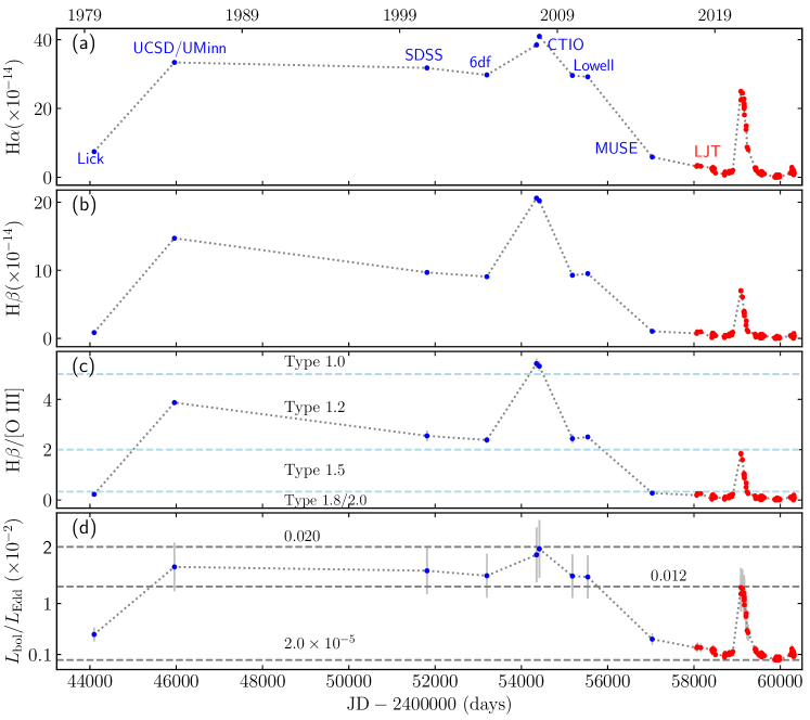
To study the evolution of AGNs, particularly the accretion disk and broad-line region evolution, we initiated a long-term observational project utilizing the Lijiang 2.4m telescope to conduct spectroscopic monitoring of a carefully selected sample of well-known AGNs. This sample includes prominent reverberation mapping AGNs (e.g., NGC 5548, see Lu2022), changing-look AGNs (e.g., Mrk 1018, Mrk 590, Mrk 993, and Mrk 883), as well as candidates for SMBH binaries (e.g., SDSS J153636.22+044127.0, which is characterized by double-peaked broad emission lines). Mrk 1018, a merger galaxy classified as Hubble type S0 (Koss2011; Veronese2024) at =0.043, was one of the earliest confirmed CL-AGNs based on limited spectroscopic observations. It exhibited a transition from type 1.9 to 1.2 over approximately five years (from 1979 to 1986; Cohen1986), before reverting back to type 1.9 in 2015 (McElroy2016). Since 2017, we have conducted follow-up spectroscopic observations of this source. In this paper, we present findings of a full-cycle CLE that occurred around 2020, along with a full-cycle AGN type transition behavior observed in Mrk 1018.
2 Observation and Data
2.1 Optical Spectroscopy and Calibration
Long-term spectroscopic observations of Mrk 1018 were conducted utilizing the Yunnan Faint Object Spectrograph and Camera (YFOSC) attached to the Lijiang 2.4 m telescope (LJT). YFOSC is quipped with a back-illuminated 20482048 pixel CCD, featuring a pixel size is 13.5 m, a pixel scale is 0.283 per pixel, a field-of-view is ), and a series of filter and Grism (Fan2015; Wang2019). For spectroscopy of Mrk 1018, Grism 14 was employed, which spans wavelengths from approximately 3600 Å to 7460 Å and offers a dispersion of 1.8 Å pixel. Following our earlier studies (Lu2021a; Lu2021b; Lu2022), a long slit with a projected width of was used, taking into account the average seeing conditions at the observatory.
The spectroscopic monitoring of Mrk 1018 started on November 5, 2017, and to date, seven-season observations have been conducted from November 2017 to February 2024 (with Modified Julian Days ranging from 58063 to 60324). Similar to the long-term spectroscopic monitoring of NGC 5548 (Lu2022), we rotated the long slit within the field of view to simultaneously capture spectra of Mrk 1018 and a nearby stable comparison star. This observational approach is commonly employed in reverberation mapping campaigns, where the spectra of the comparison star can provide high-precision spectral calibration, including flux calibration and telluric absorption corrections (e.g., see Hu2015; Lu2019a; Lu2021b and below). Standard neon and helium lamps were used for wavelength calibration. In total, we acquired 96 spectroscopic observations over an approximate duration of seven years.
We processed the two-dimensional spectroscopic data using the standard procedures in PyRAF. This involved bias subtraction, flat-field correction, wavelength calibration, and the removal of cosmic ray. Subsequently, all spectra were extracted with a consistent extraction window after subtracting the sky background. We opted for a relatively narrow extraction window of 20 pixels (5.7), which aids in minimizing Poisson noise from sky background and increasing the signal-to-noise (S/N) ratio of the spectra. The sky background was estimated from two adjacent regions ( and ) located on either side of the extraction window.
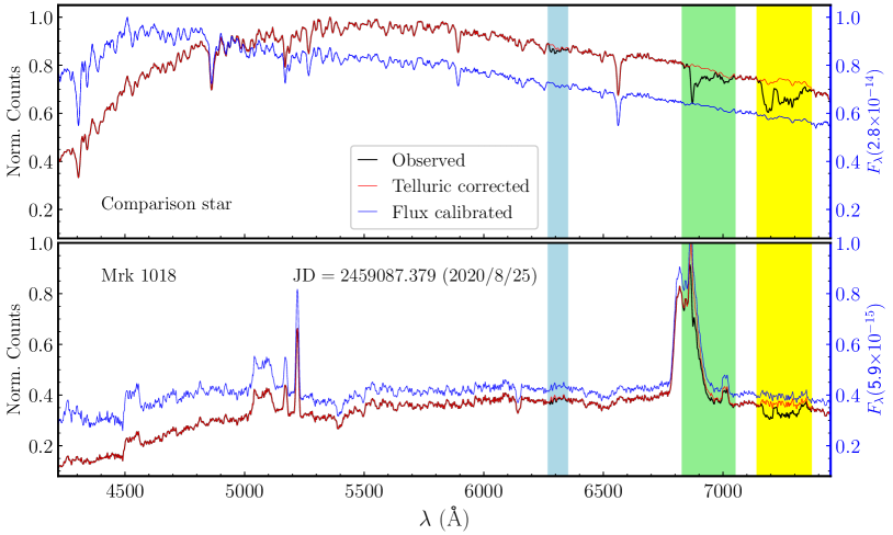
The red side of ground-based optical spectrum is contaminated by the variable absorptions of the telluric atmosphere. In the observed spectrum of Mrk 1018, there are three telluric absorption windows, which are marked by vertical colored bands in Figure 1. One of these windows (the green band) overlaps with the broad H line. We first correct the telluric absorption and subsequently calibrate the spectral fluxes.
Following the work of Lu2021b, we processed the observed spectra of Mrk 1018 through a three-step calibration procedure. First, we determined the synthesis stellar template for the comparison star by aligning its observed spectrum with a library of synthesis stellar models (e.g., Husser2013). Next, we modeled the observed spectra of comparison star (in counts) using the chosen stellar template, while masking the telluric absorption bands during this modeling (i.e., the regions marked by color diagram in Figure 1). We then derived the the telluric transmission spectra by dividing the observed spectrum of the comparison star by the modeled spectrum. This allowed us to use the telluric transmission spectra to adjust for the telluric absorption lines in each of the observed spectra. Figure 1 (left y-axis) displays the corrected spectra of telluric absorption (in red) alongside the observed spectra (in black), with the bottom panel representing the spectrum of Mrk 1018 and the top panel showing the spectrum of the comparison star. Finally, similar to the previous step, we generated a wavelength-dependent sensitivity function for each object/comparison star pair by comparing the telluric-corrected spectrum of the comparison star with the stellar template. This sensitivity function was then utilized to calibrate the spectrum of Mrk 1018 (see also Lu2019a; Lu2021a; Lu2022). The flux-calibrated spectra of Mrk 1018 (bottom panel) and its comparison star (top panel) are shown in blue in Figure 1 (right y-axis).
Before our monitoring, there exist nine spectra concurrently covering the broad H and H lines (Kim2018; Osterbrock1981; Cohen1986; Abazajian2009; Jones2009; Trippe2010; McElroy2016), which enable us to investigate the extensive long-term spectral evolution of Mrk 1018 (see Section LABEL:blrph). We obtained these early spectra from Kim2018 and recalibrated them by assuming the same [O iii] flux as our spectra. The first spectra of Mrk 1018 was taken in the 1970s, meaning that our spectroscopic baseline spans more than 45 years.
2.2 Spectral Fitting and Measurements
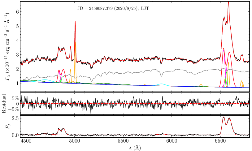
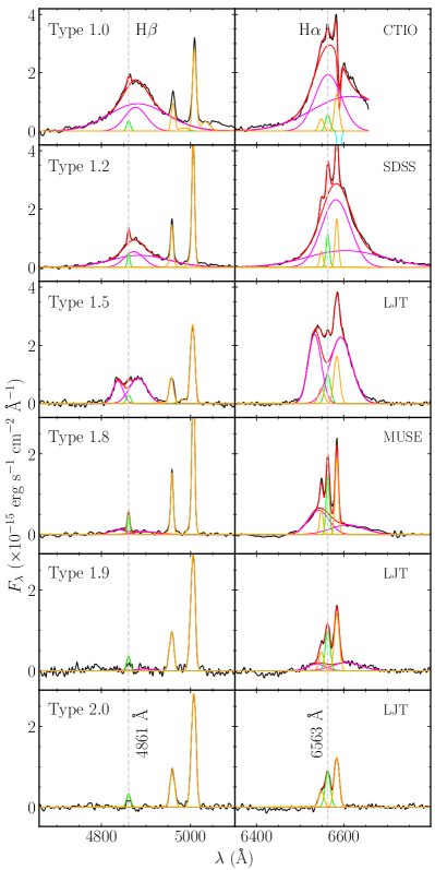
The spectral fitting scheme is commonly adopted in spectral analysis of AGNs to separate the blending components (e.g., Dong2011; Park2012; Guo2014; Barth2015). In line with previous fitting routine (e.g., Lu2022), we conducted the spectral fitting and multicomponent decomposition to extract the spectral characteristics of Mrk 1018 (see Figure 2), including variability and velocity shifts of broad emission lines. To cover the broad H and H regions while minimizing degrees of freedom, we set the fitting window from 4440 Å to 6800 Å in rest frame for all Mrk 1018 spectra. The fitting includes the following components: (1) A power law (, is the spectral index) representing the AGN continuum. (2) An iron template from Boroson1992 for the iron multiplets. (3) A stellar template with an age of 11 Gyr and metallicity of Z = 0.05 from Bruzual2003 to account for the host-galaxy starlight. (4) Double Gaussians for each broad Balmer lines (H and H). In practice, we initially attempted to fit the broad Balmer line using double Lorentzians (Lorentzian was employed for the broad Balmer line of Narrow-Line Seyfert 1 galaxies, see Veron2001), but found the fits are inferior compared to those using double Gaussians for the double-peak broad lines. Therefore, we chose to use double Gaussians to model the broad Balmer lines. (5) Two sets of double Gaussians for the [O iii] doublets 4959. (6) A single Gaussian for each narrow emission line. (7) Four sets of single Gaussian for the [S ii] doublets and the [N ii] doublets. All components were fitted simultaneously across the fitting window using the MPFIT package (Markwardt2009), which employs the LevenbergMarquardt algorithm for -minimization. During the spectral fitting for each spectrum, the flux ratio of the [O iii] doublets was fixed to the theoretical value of 3 (e.g., McGill2008; Hu2015); all the narrow emission lines were tied to the same velocity and shift, while the rest of the fitting parameters were allowed to vary. Various host-galaxy templates from Bruzual2003 were also evaluated and the template with an age of 11 Gyr and a metallicity Z = 0.05 provided a reasonable fit for the spectral index of AGNs continuum () and the stellar absorption lines. While several iron templates have been proposed for fitting the optical or ultraviolet spectra of AGNs (e.g., Boroson1992; Veron2004; Kova2010; Park2022), we found that the spectral fitting of Mrk 1018 is not sensitive to the choice of the specific iron template.
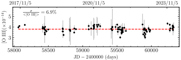
Next, we focus on the measurements of spectral characteristics. The broad H and H lines fluxes for each spectrum are measured from the optimal fitted models and are tabulated in Table 1 along with the uncertainties (including Poisson errors and systematic errors). The fluxes of the AGNs continuum can be measured from the best-fitted power-law component at 5100 Å. During our observation period, the pseudo-continuum is dominated by the starlight from the host galaxy.The mild degeneracy between power-law continuum and host-galaxy component will cause scatter to the obtained AGN continuum at 5100 Å. Therefore, we just use the averaged AGN continuum flux at 5100 Å as a a reference for the intercalibration of different photometric light curves (see Section 2.3). We measure the flux of [O iii] line from the best-fitted model and report the result in Figure 3, which exhibits a scatter of 6.9%. This level of scatter indicates a sufficient accuracy in our spectral calibration.
| JD | H | H |
|---|---|---|
| (-2,400,000 days) | () | () |
| Previous observations | ||
| 44097.500 | ||
| 45958.500 | ||
| 51812.500 | ||
| 53199.500 | ||
| 54350.500 | ||
| 54416.500 | ||
| 55182.500 | ||
| 55538.500 | ||
| 57032.500 | ||
| Our seven-season monitoring | ||
| 58063.136 | ||
| 58078.118 | ||
| 58157.048 | ||
| 58415.239 | ||
In spectral fitting described above, the broad H and H lines in each observation are well modeled by two Gaussian components, This allows us to extract the characteristics of the broad Balmer lines from the optimal models. After correcting the wavelength shift of broad Balmer lines, which usually arise from varying seeing and mis-centering, using its narrow lines as wavelength reference, we measure the peak separations of two Gaussian components (including broad H and H lines) based on the differences in peak wavelengths. Additionally, we measure the line widths including full-width at half-maximum (FWHM) and velocity dispersion () for broad H and H lines. To reasonably determine the FWHM of the double-peaked emission line, we identify a blue-side peak and a red-side peak within the line profile, and the FWHM is calculate from the maximum wavelength separation of these peaks at each half-maximum, as described by Peterson2004. In practice, instrument broadening is coupled with varying atmospheric (seeing) broadening, so we estimate the total broadening of the broad emission line for each observation by comparing the width of the [O iii] 5007 line with that from the SDSS spectrum, which is then used to derive the broadening-corrected line width. These measurements will be used to investigate the broad-line properties in subsequent analyses.
2.3 Optical Photometry and Intercalibration
To obtain the long-term variability of Mrk 1018, we compiled the photometry data from the public archival database of Zwicky Transient Facility (ZTF; Graham2019) and Asteroid Terrestrial-impact Last Alert System (ATLAS; Tonry2018). We use the ZTF - and -band data, along with the ATLAS - and -band data, and combine them using the Python package PyCALI111https://github.com/LiyrAstroph/PyCALI (LYR2014), which employs a multiplicative factor and an additive factor to intercalibrate different sources of light curves. We adopt ZTF- as the reference dataset and align other datasets with it.
2.4 Mid-infrared Photometry
Mrk 1018 is also covered by the Wide-field Infrared Survey Explorer (WISE; Wright2010) survey. We retrieved the photometric data with the following flags: the best frame image quality score (), no contamination of scattered light from the moon (), the larger South Atlantic Anomaly separation (), and spurious detections excluded (). When necessary, we convert and magnitudes into flux densities by adopting zero-point flux densities and (Jarrett2013). The resulting fluxes and magnitudes are rebinned every 6 months.
| 1979-2024 | Outburst around 2020 | ||||||
|---|---|---|---|---|---|---|---|
| (JD 2,444,097 to 2,460,324) | (JD 2,458,900 to 2,459,300) | ||||||
| Parameters | Minimum | H/[O iii]5007=0.1 | Maximum | Before the outburst | Peak | After the outburst | |
| (1) | (2) | (3) | (4) | (5) | (6) | (7) | |
| H Flux (10 erg s cm) | 0.01 | 0.75 | 40.97 | 1.32 | 24.97 | 1.41 | |
| H Luminosity (10 erg s) | 0.05 | 3.26 | 177.84 | 5.73 | 108.39 | 6.12 | |
| Luminosity at 5100 Å (10 erg s) | 0.004 | 1.26 | 39.21 | 2.04 | 25.70 | 2.16 | |
| Bolometric Luminosity (10 erg s) | 0.04 | 1.23 | 38.43 | 2.00 | 25.08 | 2.12 | |
| Eddington ratio | 2.0 | 6.1 | 0.020 | 1.0 | 0.012 | 1.0 | |
Note. — Columns (2-4) are the relevant parameters observed between 1979 and 2024 (JD 2,444,097 to 2,460,324), while columns (5-7) represent the outburst phase around 2020 (JD 2,458,900 to 2,459,300, also see Table LABEL:tab2). The optical luminosity of = was given by Greene2005, where denotes the luminosity of broad H line. Using the relation of = (McLure2004), we derive the bolometric luminosity of = erg s. Here, the cosmology with , , and is adopted.