This paper was converted on www.awesomepapers.org from LaTeX by an anonymous user.
Want to know more? Visit the Converter page.

A Serrin-type problem with
partial knowledge of the domain

Serena Dipierro Serena Dipierro: Department of Mathematics and Statistics, The University of Western Australia, 35 Stirling Highway, Crawley, Perth, WA 6009, Australia [email protected] Giorgio Poggesi Giorgio Poggesi: Department of Mathematics and Statistics, The University of Western Australia, 35 Stirling Highway, Crawley, Perth, WA 6009, Australia [email protected]  and  Enrico Valdinoci Enrico Valdinoci: Department of Mathematics and Statistics, The University of Western Australia, 35 Stirling Highway, Crawley, Perth, WA 6009, Australia [email protected] To Matilde Aurora Alessi, for inspiring us with a question on heating devices
Abstract.

We present a quantitative estimate for the radially symmetric configuration concerning a Serrin-type overdetermined problem for the torsional rigidity in a bounded domain ΩN\Omega\subset\mathbb{R}^{N}, when the equation is known on Ωω¯\Omega\setminus\overline{\omega} only, for some open subset ωΩ\omega\Subset\Omega.

The problem has concrete motivations in optimal heating with malfunctioning, laminar flows and beams with small inhomogeneities.

Key words and phrases:
Serrin’s overdetermined problem, torsional rigidity, integral identities, stability, quantitative estimates
2010 Mathematics Subject Classification:
Primary 35N25, 53A10, 35B35; Secondary 35A23

1. Introduction

In this article we consider a variation of the classical Serrin’s overdetermined problem [Se] in which the equation is only known in a subset of the domain. We will provide quantitative results showing, roughly speaking, that when the part of the domain in which we do not have information is “small”, then the domain is “close” to a ball.

1.1. Statement of the problem and main result

The precise problem that we consider may be stated as follows. Let ΩN\Omega\subset\mathbb{R}^{N} be a bounded domain – that is a bounded, open, connected set, whose boundary will be denoted by Γ\Gamma, and let ωΩ\omega\Subset\Omega be an open (not necessarily connected) subset of Ω\Omega with boundary denoted by ω\partial\omega. We consider the following problem:

(1.1) {Δu=1 in Ωω¯,u=0 on Γ,\begin{cases}\Delta u=1\quad\text{ in }\Omega\setminus\overline{\omega},\\ u=0\quad\text{ on }\Gamma,\end{cases}

under the overdetermined condition

(1.2) uν=c on Γ,u_{\nu}=c\quad\text{ on }\Gamma,

for some cc\in\mathbb{R}. Here and in what follows ν\nu denotes the outward unit normal of Ωω¯\Omega\setminus\overline{\omega} and uνu_{\nu} the derivative of uu in the direction ν\nu. Concerning the setting in (1.2), we remark that even without explicitly imposing any regularity assumptions on Γ\Gamma, [Vo, Theorem 1] guarantees that

(1.3) if (1.2) holds true (in the appropriate weak sense)then Γ is of class C2,α, with 0<α1,\begin{split}&{\mbox{if \eqref{eq:overdetermination} holds true (in the appropriate weak sense)}}\\ &{\mbox{then $\Gamma$ is of class $C^{2,\alpha}$, with~{}$0<\alpha\leq 1$,}}\end{split}

therefore the notation uνu_{\nu} on Γ\Gamma is well posed in the classical sense, being uC2,α((Ωω¯)Γ)u\in C^{2,\alpha}\left(\left(\Omega\setminus\overline{\omega}\right)\cup\Gamma\right) by standard elliptic regularity theory.

We will further assume uu to be of class C2C^{2} up to ω\partial\omega, and hence

(1.4) uC2(Ω¯ω)u\in C^{2}(\overline{\Omega}\setminus\omega)

(see Section 3 for details on this).

Concerning the regularity of the domain taken into account, to avoid unessential technicalities we will first assume that

(1.5) ω\partial\omega is of class C1C^{1}

and that

(1.6) Ωω¯ satisfies the “uniform interior sphere condition”,i.e. there exists ri>0 such that for each pΓωthere exists a ball contained in Ωω¯ of radius risuch that its closure intersects Γω only at p.\begin{split}&{\mbox{$\Omega\setminus\overline{\omega}$ satisfies the ``uniform interior sphere condition'',}}\\ &{\mbox{i.e. there exists $r_{i}>0$ such that for each $p\in\Gamma\cup\partial\omega$}}\\ &{\mbox{there exists a ball contained in $\Omega\setminus\overline{\omega}$ of radius $r_{i}$}}\\ &{\mbox{such that its closure intersects $\Gamma\cup\partial\omega$ only at $p$.}}\end{split}

We recall, for instance, that domains with C1,1C^{1,1} boundaries satisfy (1.6), see e.g. [ROV, Lemma A.1].

To state our main result we introduce some notation. For a given domain DND\subset\mathbb{R}^{N}, we denote by |D||D| and |D||\partial D| the NN-dimensional Lebesgue measure of DD and the surface measure of DD, respectively. Our main result aims at considering a convenient point zz and at obtaining suitable bounds on the “pseudo-distance”

(1.7) Γ||xz|Nc|2𝑑Sx\int_{\Gamma}\left|\frac{|x-z|}{N}-c\right|^{2}dS_{x}

and on the “asymmetry”

(1.8) |ΩΔBNc(z)||BNc(z)|,\frac{|\Omega\Delta B_{Nc}(z)|}{|B_{Nc}(z)|},

where ΩΔBNc(z)\Omega\Delta B_{Nc}(z) denotes the symmetric difference of Ω\Omega and the ball BNc(z)B_{Nc}(z) of radius NcNc centered at zz. In addition, we provide a “geometric” bound on the set by estimating the difference between the largest ball centered at zz contained in Ω\Omega and the smallest ball centered at zz that contains Ω\Omega.

The precise result that we have here goes as follows:

Theorem 1.1.

Let Ωω¯N\Omega\setminus\overline{\omega}\subset\mathbb{R}^{N} be a bounded domain satisfying assumptions (1.5) and (1.6). Let uu satisfy (1.1), (1.2) and (1.4). Assume that u0u\leq 0 on ω\partial\omega. Set

(1.9) z:=1|Ωω¯|{Ωω¯x𝑑xNωuν𝑑Sx}.z:=\frac{1}{|\Omega\setminus\overline{\omega}|}\left\{\int_{\Omega\setminus\overline{\omega}}x\,dx-N\int_{\partial\omega}u\;\nu\,dS_{x}\right\}.

Then,

(1.10) Γ||xz|Nc|2𝑑SxC|ω|\int_{\Gamma}\left|\frac{|x-z|}{N}-c\right|^{2}dS_{x}\leq C|\partial\omega|

and

(1.11) |ΩΔBNc(z)||BNc(z)|C|ω|1/2.\frac{|\Omega\Delta B_{Nc}(z)|}{|B_{Nc}(z)|}\leq C|\partial\omega|^{1/2}.

In (1.10) and (1.11), the quantity CC denotes a positive constant depending only on the dimension NN, on the internal radius rir_{i} in (1.6), on the diameter of Ω\Omega, and on uC2(ω)\|u\|_{C^{2}(\partial\omega)}.

Moreover, if

(1.12) zΩ,z\in\Omega,

then there exist ρeρi>0\rho_{e}\geq\rho_{i}>0 such that

(1.13) Bρi(z)ΩBρe(z)B_{\rho_{i}}(z)\subset\Omega\subset B_{\rho_{e}}(z)

and

(1.14) ρeρiC|ω|τN/2,\rho_{e}-\rho_{i}\leq C\,|\partial\omega|^{\tau_{N}/2},

where CC is a positive constant depending only on the dimension NN, on the internal radius rir_{i} in (1.6), on the diameter of Ω\Omega and on uC2(ω)\|u\|_{C^{2}(\partial\omega)}, and τN>0\tau_{N}>0 is a constant depending only on NN.

We point out that Theorem 1.1 collects three different aspects on the problem: indeed, the statement in (1.10) is an “integral” stability result in L2L^{2} (see Section 5), the estimate in (1.11) provides a stability “in measure”, and the result in (1.14) deals with a “pointwise” notion of stability.

The exponent τN\tau_{N} in (1.14) can be better precised. Indeed, we can take

τ2:=1.\tau_{2}:=1.

Moreover, τ3\tau_{3} can be taken arbitrarily close to one, in the sense that for any θ>0\theta>0, we have that (1.14) holds with τ3:=1θ\tau_{3}:=1-\theta and CC depending also on θ\theta.

Furthermore, for N4N\geq 4, we can take

τN:=2N1.\tau_{N}:=\frac{2}{N-1}.

We think that it is an interesting open problem to detect whether these choices of exponents τ2\tau_{2}, τ3\tau_{3}, τN\tau_{N} in (1.14), as well as the exponents appearing in (1.10) and (1.11), are optimal in Theorem 1.1. It would also be very interesting to have explicit examples to check the optimality of the structural assumptions in Theorem 1.1.

We also point out that condition (1.12) is naturally satisfied in many concrete situations (see also Remark 7.2): in particular, for “small” ω\omega, the point zz is “close” to the baricenter of Ω\Omega, hence condition (1.12) is fulfilled in this case when the baricenter of Ω\Omega lies in Ω\Omega (as it happens, for instance, for convex sets).

Of course, when ω=\omega=\varnothing, we have that (1.14) reduces to ρe=ρi\rho_{e}=\rho_{i} and therefore (1.13) gives that Ω\Omega is a ball: in this sense Theorem 1.1 recovers the classical results of [Se, We] for overdetermined problems. The main difference here is that, differently from the existing literature, the equation is supposed to hold possibly only outside a subdomain ω\omega: as a counterpart, Theorem 1.1 does not prove that the full domain is a ball, but only that it is geometrically close to a ball whenever the subdomain ω\omega has a small Lebesgue measure.

In the present setting, Theorem 1.1 will be in fact a particular case of more general quantitative results, presented in Section 7, and relying on a number of auxiliary integral identities. For more details, see Theorems 7.1, 7.3, 7.4, and 7.6.

In this spirit, Theorem 1.1 falls within the broad stream of research aiming at obtaining quantitative rigidity results, see e.g. [ABR, BNST, CMV, CV1, Fe, Ma, MP1, MP2, MP3, Pog2] and the references therein. More generally, overdetermined problems have been also considered e.g. in [AB, CV2, EP, FV1, FV2, FV3, FV4, FG, FGK, FGLP, MR1808686, MR2002730, GL, GS, GX, PS, Pog] and in the references therein.

1.2. Comments on the structural assumptions and generalizations

We remark that assumption (1.6) gives a lower bound on the distance not only between ω\partial\omega and Γ\Gamma (being dist(ω,Γ)2ri\mathop{\mathrm{dist}}(\partial\omega,\Gamma)\geq 2r_{i}), but also between the boundaries of the different connected components of ω\omega (if any).

Interestingly, assumptions (1.5) and (1.6) can be relaxed, as explained in Section 8.

In particular, suitable counterparts of (1.10) and (1.11) can be obtained if (1.5) and (1.6) are replaced by the weaker assumptions

(1.15) Ωω¯\Omega\setminus\overline{\omega} is a John domain

and

(1.16) Ωω¯\Omega\setminus\overline{\omega} is of finite perimeter.

Moreover, a counterpart of the pointwise estimate (1.14) can be obtained if (1.5) and (1.6) are dropped and replaced by (1.15), (1.16), and the assumption

(1.17) Ωω¯ satisfies the “uniform interior sphere condition only on Γ”,i.e., there exists ri>0 such that for each pΓ there existsa ball contained in Ωω¯ of radius ri such that its closureintersects Γω only at p on Γ.\begin{split}&{\mbox{$\Omega\setminus\overline{\omega}$ satisfies the ``uniform interior sphere condition only on $\Gamma$'',}}\\ &{\mbox{i.e., there exists $r_{i}>0$ such that for each $p\in\Gamma$ there exists}}\\ &{\mbox{a ball contained in $\Omega\setminus\overline{\omega}$ of radius $r_{i}$ such that its closure}}\\ &{\mbox{intersects $\Gamma\cup\partial\omega$ only at $p$ on $\Gamma$.}}\end{split}

We stress that (1.17) is equivalent to assume a lower bound only for dist(ω,Γ)\mathop{\mathrm{dist}}(\partial\omega,\Gamma). Indeed, being Γ\Gamma of class C2,αC^{2,\alpha}, the set Ω\Omega surely satisfies the uniform interior sphere condition on Γ\Gamma.

In this situation, Theorem 1.1 remains valid, with the following structural modifications:

  • The boundary measure of ω\partial\omega is replaced by its perimeter, namely by the (N1)(N-1)-dimensional Hausdorff measure N1(ω){\mathcal{H}}^{N-1}(\partial^{*}\omega) of its reduced boundary ω\partial^{*}\omega. In turn, ν\nu on ω\partial^{*}\omega has to be intended as the (measure-theoretic) outer unit normal (see Section 8).

  • The constants CC depend on rir_{i} defined in (1.17) and on the structural constant b0b_{0} of the given b0b_{0}-John domain;

  • The explicit expression of the exponents τN\tau_{N} in the pointwise estimate (1.14) is possibly worse than the ones obtained in Theorem 1.1.

The definition and details for b0b_{0}-John domains can be found in Subsection 8.1. Here, we just stress that the class of John domains is huge: in particular, if (1.6) is satisfied then Ωω¯\Omega\setminus\overline{\omega} is surely a b0b_{0}-John domain with b0dΩ/rib_{0}\leq d_{\Omega}/r_{i} (see [Pog2, (iii) of Remark 3.12]).

The precise statement that we have in this framework is stated next, and can be deduced from more general results presented in Theorems 8.3, 8.6, 8.9 and 8.10.

Theorem 1.2.

Let Ωω¯N\Omega\setminus\overline{\omega}\subset\mathbb{R}^{N} be a bounded domain satisfying assumptions (1.15) and (1.16). Let uu satisfy (1.1), (1.2) and (1.4). Assume that u0u\leq 0 on ω\partial\omega. Set

z:=1|Ωω¯|{Ωω¯x𝑑xNωuν𝑑N1}.z:=\frac{1}{|\Omega\setminus\overline{\omega}|}\left\{\int_{\Omega\setminus\overline{\omega}}x\,dx-N\int_{\partial^{*}\omega}u\;\nu\,d{\mathcal{H}}^{N-1}\right\}.

Then, the pseudodistance defined in (1.7) and the asymmetry defined in (1.8) satisfy

(1.18) Γ||xz|Nc|2𝑑N1CN1(ω),\int_{\Gamma}\left|\frac{|x-z|}{N}-c\right|^{2}\,d{\mathcal{H}}^{N-1}\leq C{\mathcal{H}}^{N-1}(\partial^{*}\omega),
(1.19) |ΩΔBNc(z)||BNc(z)|CN1(ω)1/2,\frac{|\Omega\Delta B_{Nc}(z)|}{|B_{Nc}(z)|}\leq C{\mathcal{H}}^{N-1}(\partial^{*}\omega)^{1/2},

where the constants C>0C>0 appearing in (1.18) and (1.19) depend only on NN, b0b_{0}, dΩd_{\Omega}, cc, and uC2(ω)\|u\|_{C^{2}(\partial\omega)}.

If in addition (1.17) is verified and zΩz\in\Omega, then there exist ρeρi>0\rho_{e}\geq\rho_{i}>0 such that

Bρi(z)ΩBρe(z)B_{\rho_{i}}(z)\subset\Omega\subset B_{\rho_{e}}(z)

and

(1.20) ρeρiC(N1(ω))τN/2,\rho_{e}-\rho_{i}\leq C\,\big{(}{\mathcal{H}}^{N-1}(\partial^{*}\omega)\big{)}^{\tau_{N}/2},

where C>0C>0 is a constant depending only on NN, the internal radius rir_{i} in (1.17), dΩd_{\Omega}, b0b_{0}, and on uC2(ω)\|u\|_{C^{2}(\partial\omega)}. The exponents τN>0\tau_{N}>0 depend only on NN.

We point out that in Theorem 1.2 we maintained the “same” choice (1.9) for the point zz.

The dependence of the constants CC on cc in (1.18) and (1.19) could be replaced with the dependence on the surface measure |Γ||\Gamma|, as explained in Remark 8.11.

The explicit values of τN\tau_{N} in (1.20) are the following ones. We have that τ2\tau_{2} can be taken as close as we wish to 11, namely one can fix any θ>0\theta>0 and take τ2:=1θ\tau_{2}:=1-\theta (in this case, the constant CC in (1.20) will also depend on θ\theta). When N3N\geq 3, one can take τN:=2N\tau_{N}:=\frac{2}{N}.

We notice that these exponents are all smaller (i.e., “worse”) than the ones obtained in Theorem 1.1. Nevertheless, it is possible to get the pointwise estimate (1.20) with the better exponents τN\tau_{N} obtained in (1.14), and by removing the John condition (1.15), provided that we make a different choice of zz.

The precise statement, that can be deduced from more general results obtained in Theorems 8.15 and 8.16, is the following:

Theorem 1.3.

Let Ωω¯N\Omega\setminus\overline{\omega}\subset\mathbb{R}^{N} be a bounded domain satisfying assumptions (1.16) and (1.17). Let uu satisfy (1.1), (1.2) and (1.4). Assume that u0u\leq 0 on ω\partial\omega. Set

(1.21) z:=1|Ωric|{Ωricx𝑑xNΓriuν𝑑Sx},z:=\frac{1}{|\Omega^{c}_{r_{i}}|}\left\{\int_{\Omega^{c}_{r_{i}}}x\,dx-N\int_{\Gamma_{r_{i}}}u\;\nu\,dS_{x}\right\},

where Ωric\Omega^{c}_{r_{i}} denotes the points in Ω\Omega which lie at distance strictly less than rir_{i} from Γ\Gamma, and Γri\Gamma_{r_{i}} denotes the points in Ω\Omega which lie at distance rir_{i} from Γ\Gamma.

If zΩz\in\Omega, then there exist ρeρi>0\rho_{e}\geq\rho_{i}>0 such that

Bρi(z)ΩBρe(z)B_{\rho_{i}}(z)\subset\Omega\subset B_{\rho_{e}}(z)

and

ρeρiC(N1(ω))τN/2,\rho_{e}-\rho_{i}\leq C\,\big{(}{\mathcal{H}}^{N-1}(\partial^{*}\omega)\big{)}^{\tau_{N}/2},

where C>0C>0 is a constant depending only on NN, the internal radius rir_{i} in (1.17), dΩd_{\Omega}, and uC2(ω)\|u\|_{C^{2}(\partial\omega)}. The exponents τN>0\tau_{N}>0 depend only on NN.

We stress that the approach used in Theorem 1.3 does not need the assumption in (1.15) that Ωω¯\Omega\setminus\overline{\omega} is a John domain and hence the dependence on b0b_{0}, present in (1.20), has been dropped.

Interestingly, the values of the exponents τN\tau_{N} in Theorem 1.3 are the same as those in Theorem 1.1 (and therefore they are “better” than the ones obtained in (1.20), though they rely on a different choice of zz).

We think that it would be interesting to investigate the possible optimality of these exponents also in the framework provided by Theorem 1.3.

We remark that the setting of zz in (1.21) is modeled on the annular set Ωric\Omega^{c}_{r_{i}} rather than on Ωω¯\Omega\setminus\overline{\omega} as in (1.9). It would be interesting to further investigate the impact of different possible choices for zz.

1.3. Organization of the paper

The rest of this paper is organized as follows. Section 2 contains some detailed motivations from shape optimization, fluid dynamics and mechanics which naturally lead to the problem considered in this paper.

In Section 3 we make some notation precise.

In Section 4, we present some integral identities of Rellich-Pohozaev-type for solutions of (1.1). In these computations, one does not need to impose the additional condition in (1.2) from the beginning, and aims at comparing a weighted “deficit” on Ωω¯\Omega\setminus\overline{\omega} (measuring “how far from rotational invariant” the solution is) with suitable surface integrands on Γ\Gamma and ω\partial\omega. From these identities, the auxiliary information in (1.2) provides a more precise, and simpler information.

In Section 5 we collect useful estimates and we use them to obtain a suitable stability bound on the spherical pseudo-distance defined in (1.7) (see Theorem 5.7). We also put in relation this pseudo-distance with the asymmetry defined in (1.8) (see Lemma 5.1).

The estimates collected in Section 5 are then also used in Section 6 to bound the difference ρeρi\rho_{e}-\rho_{i}.

In Section 7, from the information obtained in Sections 5 and 6, we obtain a number of quantitative results, that also contain Theorem 1.1 as a particular case.

Finally, in Section 8 we obtain generalizations of the quantitative results presented in Section 7, by relaxing the regularity assumptions (1.5) and (1.6), and hence we establish Theorems 1.2 and 1.3 as particular cases.

2. Models and motivations

2.1. Heating with source malfunctioning

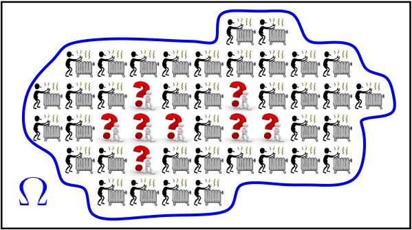
A natural motivation for problem (1.1)-(1.2) comes from the optimal heating theory. In this setting, a region Ω\Omega is given which is in direct contact with an external environment having constant (say, zero) temperature. In this setting, at the equilibrium, the temperature on the boundary of Ω\Omega is set to be zero. The region Ω\Omega is also provided by a fine set of heating devices. All these devices are the same and produce the same heating effect with the exception of those placed in a small subregion ω\omega which are malfunctioning, see Figure 1.

Refer to caption
Figure 1. Matilde’s problem: a region with some malfunctioning heating devices.

In this setting, at the equilibrium, the local heat flow, normalized by the flow surface, is constant, say equal to 11, in Ωω\Omega\setminus\omega, but it may be different from 11 in ω\omega. In a nutshell, the mathematical description of this situation is given by

(2.1) {Δu=f in Ω,u=0 on Ω,\begin{cases}\Delta u=f&{\mbox{ in }}\Omega,\\ u=0&{\mbox{ on }}\partial\Omega,\end{cases}

with f(x)=1f(x)=1 for every xΩωx\in\Omega\setminus\omega.

A natural question in this setting is to optimize the shape of Ω\Omega in order to store in the domain the biggest possible amount of caloric energy. Concretely, given u=u(f)u=u^{(f)} satisfying (2.1), one may try to select Ω\Omega in order to maximize (among the domains of fixed measure) the functional

(2.2) Ω|u(f)(x)|2𝑑x.\int_{\Omega}|\nabla u^{(f)}(x)|^{2}\,dx.

This variational problem is well posed (see e.g. Theorem 4.5.2 in [HP]) and it is naturally related to the boundary derivative prescription

(2.3) νu(f)=const\partial_{\nu}u^{(f)}={\rm const} on Ω\partial\Omega,

thus leading to the problem described in (1.1)-(1.2). We refer to Proposition 6.1.10 in [HP] and Appendix A here for a direct computation relating the shape optimization of (2.2) and the Neumann condition in (2.3).

In this framework, our result111Strictly speaking, (2.1) with a source f0f\geq 0 should be described as an optimal cooling, rather than heating, problem: speaking of heating problem should require to add a minus sign in front of Δ\Delta in (2.1). Nevertheless, we preferred to keep the sign convention in accordance with (1.1) and the rest of the paper. in Theorem 1.1 states that, for a small region ω\omega of malfunctioning of the heat source, the optimal domain Ω\Omega is necessarily close to a ball (with a quantitative information on the proximity between Ω\Omega and a suitable ball). This result is close to intuition, since jagged domains end up dissipating most of the caloric energy from their boundaries.

2.2. Laminar flows with a small tube of unknown density

Another motivation of the problem in (1.1)-(1.2) comes from laminar flows, as modeled by a Navier-Stokes equation of the type

(2.4) t(ρv)+div(ρvv)μΔv+p=ρg,\partial_{t}(\rho v)+{\rm div}(\rho v\otimes v)-\mu\Delta v+\nabla p=-\rho g,

where vv is the vectorial velocity of the fluid, ρ\rho is its density, μ\mu is its viscosity coefficient, pp is the pressure, gg is the gravity acceleration and \otimes denotes the outer product (i.e., given two vectors aa and bb, aba\otimes b is the matrix whose (i,j)(i,j)th entry is aibja_{i}b_{j}) see e.g. [Da]. The incompressibility condition

(2.5) divv=0{\rm div}\,v=0

leads to

div(ρvv)=(v)(ρv).{\rm div}(\rho v\otimes v)=(v\cdot\nabla)(\rho v).

In this way, one obtains from (2.4) that

(2.6) t(ρv)+(v)(ρv)μΔv+p=ρg.\partial_{t}(\rho v)+(v\cdot\nabla)(\rho v)-\mu\Delta v+\nabla p=-\rho g.

One assumes that the flow is “vertical”, namely v=(0,0,u)v=(0,0,u) for some scalar function uu, thus obtaining that

(2.7) (v)(ρv)=((0,0,u))(ρ(0,0,u))=u3(ρ(0,0,u)).(v\cdot\nabla)(\rho v)=((0,0,u)\cdot\nabla)(\rho(0,0,u))=u\,\partial_{3}(\rho(0,0,u)).

We also suppose that the laminar flow occurs in a “vertical tube” of the type Ω×\Omega\times\mathbb{R}, with Ω2\Omega\subset\mathbb{R}^{2}, and that the density of the fluid only depends on the horizontal position (that is, the fluid maintains the same density along its vertical flow). In this setting, we have that ρ=ρ(x1,x2)\rho=\rho(x_{1},x_{2}) and accordingly, by (2.5) and (2.7),

(v)(ρv)=(0,0,ρu3u)=(0,0,ρudivv)=0.(v\cdot\nabla)(\rho v)=(0,0,\rho u\,\partial_{3}u)=(0,0,\rho u\,{\rm div}\,v)=0.

Hence, we deduce from the third component of (2.6) that

(2.8) ρtuμΔu+3p=ρg.\rho\partial_{t}u-\mu\Delta u+\partial_{3}p=-\rho g.

The case of a “steady state” flow (that is tu=0\partial_{t}u=0) with constant pressure (hence 3p=0\partial_{3}p=0) reduces (2.8) to

(2.9) Δu=ρgμ.\Delta u=\frac{\rho g}{\mu}.

If the fluid has constant (say, up to changing the inertial reference frame, zero) velocity at the boundary of the pipe, equation (2.9) is complemented by the boundary condition

(2.10) u=0on Ω.u=0\qquad{\mbox{on }}\partial\Omega.

Also, if the fluid presents a constant tangential stress on the pipe, we have that

(2.11) νu=constanton Ω.\partial_{\nu}u={\rm constant}\qquad{\mbox{on }}\partial\Omega.

The case described in (1.1)-(1.2) is, in this setting, a byproduct of (2.9), (2.10) and (2.11) in which the density of the fluid (as well as its viscosity and the gravity acceleration) is constant in the region Ωω¯\Omega\setminus\overline{\omega}, but it is possibly unknown in ω\omega. In this framework, our result in Theorem 1.1 says that if a laminar fluid is homogeneous out of a small region and presents a constant tangential stress on the pipe, then necessarily the pipe is close to a right circular cylinder.

2.3. Traction of beams with small inhomogeneity

In the theory of elasticity, one can consider the displacement vector U=(U1,U2,U3)U=(U_{1},U_{2},U_{3}) that describes the deformation of some material. Also, it is customary to introduce the stress tensor

(2.12) σij:=iUj+jUi,\sigma_{ij}:=\partial_{i}U_{j}+\partial_{j}U_{i},

describing the force (per unit area) in the iith direction along the infinitesimal surface orthogonal to eje_{j}, being e1:=(1,0,0)e_{1}:=(1,0,0), e2:=(0,1,0)e_{2}:=(0,1,0) and e3:=(0,0,1)e_{3}:=(0,0,1), see e.g. formula (129) in [Hj] (here, we are supposing the strain and the stress to be proportional, setting the proportionality constant equal to 11 for the sake of simplicity).

In this framework, the equilibrium configurations are those for which the forces are infinitesimally balanced, that is

(2.13) j=13jσij=0for all i{1,2,3},\sum_{j=1}^{3}\partial_{j}\sigma_{ij}=0\qquad{\mbox{for all }}i\in\{1,2,3\},

see e.g. formula (189) in [Hj].

More specifically, we focus here on the torsion of a vertical beam {\mathcal{B}} (see e.g. [So, pages 100-120]). The fact that the beam is vertical means, in our setting, that

(2.14) ={(x1,x2,x3) s.t. (x1,x2)Ωx3},{\mathcal{B}}=\{(x_{1},x_{2},x_{3}){\mbox{ s.t. }}(x_{1},x_{2})\in\Omega_{x_{3}}\},

for a suitable (bounded and smooth) family of domains Ωx32\Omega_{x_{3}}\subset\mathbb{R}^{2}. We assume that each point of the beam lying on a given horizontal plane {x3=x¯3}\{x_{3}=\bar{x}_{3}\} performs a horizontal rotation of a small angle ϑ=ϑ(x)\vartheta=\vartheta(x), plus a vertical movement that is the same for every height of the bar (we will denote this vertical movement by v=v(x1,x2)v=v(x_{1},x_{2})). In this setting, the torsion of the bar moves a point x=(x1,x2,x¯3)x=(x_{1},x_{2},\bar{x}_{3}) to the point

X:=(x1cosϑ+x2sinϑ,x1sinϑ+x2cosϑ,x¯3+v)(x1+x2ϑ,x1ϑ+x2,x¯3+v),X:=(x_{1}\cos\vartheta+x_{2}\sin\vartheta,-x_{1}\sin\vartheta+x_{2}\cos\vartheta,\bar{x}_{3}+v)\simeq(x_{1}+x_{2}\vartheta,-x_{1}\vartheta+x_{2},\bar{x}_{3}+v),

and so, in this approximation, we can write the displacement vector as

U=Xx=(ϑx2,ϑx1,v).U=X-x=(\vartheta\,x_{2},-\vartheta\,x_{1},v).

From this and (2.12), we can write

(2.15) σ31=3U1+1U3=3ϑx2+1v,σ32=3U2+2U3=3ϑx1+2v,andσ33=23U3=0.\begin{split}&\sigma_{31}=\partial_{3}U_{1}+\partial_{1}U_{3}=\partial_{3}\vartheta\,x_{2}+\partial_{1}v,\\ &\sigma_{32}=\partial_{3}U_{2}+\partial_{2}U_{3}=-\partial_{3}\vartheta\,x_{1}+\partial_{2}v,\\ {\mbox{and}}\qquad&\sigma_{33}=2\partial_{3}U_{3}=0.\end{split}

As a result, exploiting the latter equation and (2.13) with i:=3i:=3,

(2.16) 0=j=13jσ3j=1σ31+2σ32.0=\sum_{j=1}^{3}\partial_{j}\sigma_{3j}=\partial_{1}\sigma_{31}+\partial_{2}\sigma_{32}.

We then fix x3=1x_{3}=1 and consider the 11-form on 2\mathbb{R}^{2} given by

(2.17) α:=σ32dx1+σ31dx2,\alpha:=-\sigma_{32}\,dx_{1}+\sigma_{31}\,dx_{2},

and we deduce from (2.16) that

dα=(2σ32+1σ31)dx1dx2=0.d\alpha=\big{(}\partial_{2}\sigma_{32}+\partial_{1}\sigma_{31}\big{)}\,dx_{1}\wedge dx_{2}=0.

This gives that there exists a “warping potential” uu such that α=du\alpha=du as 11-forms in 2\mathbb{R}^{2}. Accordingly, by (2.17), we have that

(2.18) 1u=σ32and2u=σ31.\partial_{1}u=-\sigma_{32}\qquad{\mbox{and}}\qquad\partial_{2}u=\sigma_{31}.

Combining this with (2.15), one sees that

1u=3ϑx12vand2u=3ϑx2+1v,\partial_{1}u=\partial_{3}\vartheta\,x_{1}-\partial_{2}v\qquad{\mbox{and}}\qquad\partial_{2}u=\partial_{3}\vartheta\,x_{2}+\partial_{1}v,

and therefore

(2.19) Δu=1(3ϑx12v)+2(3ϑx2+1v)=23ϑ+1,32ϑx1+2,32ϑx2,\Delta u=\partial_{1}\big{(}\partial_{3}\vartheta\,x_{1}-\partial_{2}v\big{)}+\partial_{2}\big{(}\partial_{3}\vartheta\,x_{2}+\partial_{1}v\big{)}=2\partial_{3}\vartheta+\partial^{2}_{1,3}\vartheta\,x_{1}+\partial^{2}_{2,3}\vartheta\,x_{2},

with these functions evaluated at x3=1x_{3}=1. As a special case, one can take into account the situation in which the angle ϑ\vartheta depends linearly on the height of the beam, say ϑ(x)=θ(x1,x2)x3\vartheta(x)=\theta(x_{1},x_{2})\,x_{3} (this is physically reasonable, for instance, if the beam is constrained at {x3=0}\{x_{3}=0\} and some torque is applied from the top of the beam). In this setting, (2.19) reduces to

(2.20) Δu=2θ+1θx1+2θx2.\Delta u=2\theta+\partial_{1}\theta\,x_{1}+\partial_{2}\theta\,x_{2}.

If we suppose that the beam is built by two different materials, one occupying Ωω¯\Omega\setminus\overline{\omega} and the other occupying ω\omega (where Ω\Omega here represents the domain Ωx3\Omega_{x_{3}} in (2.14) with x3=1x_{3}=1), the expression in (2.20) takes two different forms in Ωω¯\Omega\setminus\overline{\omega} and ω\omega. In particular, if we know that the material in Ωω¯\Omega\setminus\overline{\omega} is homogeneous we can suppose that the horizontal rotation is uniform there and thus θ\theta is independent on the point (i.e., 1θ=2θ=0\partial_{1}\theta=\partial_{2}\theta=0), hence deducing from (2.20) that

(2.21) Δu=constantin Ωω¯.\Delta u={\rm constant}\qquad{\mbox{in }}\Omega\setminus\overline{\omega}.

Also, the surface traction, as a force per unit of area, at a boundary point of the beam is defined as the normal component of the vertical stress, that is

T:=(σ31,σ32,σ33)ν¯,T:=(\sigma_{31},\sigma_{32},\sigma_{33})\cdot\bar{\nu},

being ν¯3\bar{\nu}\in\mathbb{R}^{3} the normal to the beam (see e.g. the third component in formula (174) of [Hj]). Recalling (2.15), we have that

T=(σ31,σ32,0)ν¯=(σ31,σ32)ν,T=(\sigma_{31},\sigma_{32},0)\cdot\bar{\nu}=(\sigma_{31},\sigma_{32})\cdot\nu,

being ν2\nu\in\mathbb{R}^{2} normal to Ω\Omega. Thus, in view of (2.18),

T=(2u,1u)ν=uτ,T=(\partial_{2}u,-\partial_{1}u)\cdot\nu=\nabla u\cdot\tau,

being τ:=(ν2,ν1)\tau:=(-\nu_{2},\nu_{1}) a unit tangent vector to Ω\Omega. Therefore, if the traction vanishes, the tangential derivative of uu vanishes as well, hence uu is constant along Ω\partial\Omega. Since uu was introduced as a potential, it is defined up to an additive constant, hence we can rephrase these considerations by saying that if the traction vanishes, then

(2.22) u=0on Ω.u=0\qquad{\mbox{on }}\partial\Omega.

We also remark that, if σ3=(σ31,σ32,σ33)\sigma_{3}=(\sigma_{31},\sigma_{32},\sigma_{33}), then

|σ3|=|(σ31,σ32,0)|=|u|,|\sigma_{3}|=|(\sigma_{31},\sigma_{32},0)|=|\nabla u|,

thanks to (2.15) and (2.18).

Hence, for constant stress intensity |σ3||\sigma_{3}|, we deduce from (2.22) that

(2.23) νu=constanton Ω.\partial_{\nu}u={\mbox{constant}}\qquad{\mbox{on }}\partial\Omega.

We thus observe that problem (1.1)-(1.2) arises naturally from (2.21), (2.22) and (2.23), and, in this framework, Theorem 1.1 says that if a beam is homogeneous out of a small region and presents zero traction and constant stress intensity, then necessarily the horizontal section of the beam is close to a disk.

3. Notation

Unless differently specified, we will denote by ΩN\Omega\subset\mathbb{R}^{N}, with N2N\geq 2, a connected, bounded open set, and call Γ:=Ω\Gamma:=\partial\Omega its boundary. We will denote indifferently by |Ω||\Omega| and |Γ||\Gamma| the NN-dimensional Lebesgue measure of Ω\Omega and the surface measure of Γ\Gamma.

Moreover, we will denote by dΩd_{\Omega} the diameter of Ω\Omega, that is

(3.1) dΩ:=supx,yΩ|xy|.d_{\Omega}:=\sup_{x,y\in\Omega}|x-y|.

Also, we shall denote by ω\omega an open subset of Ω\Omega, such that ω¯Ω\overline{\omega}\subset\Omega.

For all xΩω¯x\in\Omega\setminus\overline{\omega}, we consider the distance function

(3.2) δ(x):=dist(x,Γω).\delta(x):=\mathop{\mathrm{dist}}(x,\Gamma\cup\partial\omega).

As already mentioned in the Introduction, we first consider the case in which, being (1.5) in force and by recalling (1.3), Ωω¯\Omega\setminus\overline{\omega} is of class C1C^{1}: in this setting ν\nu denotes the (exterior) unit normal vector field to Ωω¯\Omega\setminus\overline{\omega}. Then, we will clarify in Section 8 the notation that we use when the regularity assumption in (1.5) is dropped.

Now, we clarify the notation used for the spaces CkC^{k} and we discuss the regularity assumption in (1.4).

As usual, for an open set DND\subset\mathbb{R}^{N}, and kk a positive integer, Ck(D)C^{k}(D) denotes the space of functions possessing continuous derivatives up to order kk on DD.

By Ck(D¯)C^{k}(\overline{D}) we denote the space of functions that are restrictions to D¯\overline{D} of functions in Ck(N)C^{k}(\mathbb{R}^{N}). In other words, Ck(D¯)C^{k}(\overline{D}) is the space of the functions in Ck(D)C^{k}(D) that can be extended to Ck(N)C^{k}(\mathbb{R}^{N}). The same definition has been adopted for instance in [Leoni, Appendix C, pag. 562] and also in many books of Differential Geometry.

We recall that, thanks to Whitney extension theorem (see the original paper [Wh] or [KP-Primer, Theorem 2.3.6]), this definition is equivalent to [KP-Primer, Definition 2.3.5] based on a Taylor-expansion condition.

Moreover, if DD satisfies property (P) of [Wh-boundaries] – i.e., quasiconvexity, that in particular is surely satisfied if DD is Lipschitz (see [Br, Sections 2.5.1, 2.5.2]) – then, thanks to the main theorem on page 485 in [Wh-boundaries], our definition of Ck(D¯)C^{k}(\overline{D}) (as well as [KP-Primer, Definition 2.3.5]) is also equivalent to the definition used in many books of PDEs (e.g., [GT]), that is: Ck(D¯)C^{k}(\overline{D}) is the space of functions in Ck(D)C^{k}(D) whose derivatives up to order kk have continuous extensions to the closure D¯\overline{D}.

For more general domains, [KP-Primer, Definition 2.3.5] (as well as our definition) is stronger than that adopted in [GT]. For more details on this subject we refer to [KP-Primer, Section 2.3], [KP, Section 5.2], [Kra], [Br], and [Leoni, Appendix C].

In our setting, by taking D:=Ωω¯D:=\Omega\setminus\overline{\omega} and k:=2k:=2 in the definition of Ck(D¯)C^{k}(\overline{D}), we have that the assumption in (1.4) guarantees that uu can be extended to a C2C^{2} function throughout N\mathbb{R}^{N}. This will allow us to perform the generalizations described in Section 8 when the regularity assumption on ω\partial\omega in (1.5) is dropped and replaced just by (1.16). In particular, when integrating by parts, we can still write the derivatives of uu up to the second order on the reduced boundary ω\partial^{*}\omega.

We remark that up to Section 7, we will take Ωω¯\Omega\setminus\overline{\omega} to be of class C1C^{1}, and therefore assumption (1.4) has univocal meaning, no matter what definition of C2(Ω¯ω)C^{2}(\overline{\Omega}\setminus\omega) we adopt (among the three presented above).

4. Integral identities

The goal of this section is to develop a series of integral identities which will be conveniently exploited to deduce quantitative bounds on the solution of (1.1)-(1.2) and on its domain of definition. We start by proving a Rellich-Pohozaev-type identity and its consequences. Notice that in the next two statements we are not imposing yet the overdetermined condition in (1.2).

Lemma 4.1 (A Rellich-Pohozaev-type identity).

Suppose that Ωω¯\Omega\setminus\overline{\omega} is of class C1C^{1}. If uC2(Ω¯ω)u\in C^{2}(\overline{\Omega}\setminus\omega) satisfies (1.1), then the following identity holds:

(4.1) (N+2)Ωω¯|u|2𝑑x=Γ<x,ν>uν2dSx+2Nω{uuν<x,ν>Nu+<x,u>Nuν<x,ν>2N|u|2}𝑑Sx.\begin{split}&(N+2)\int_{\Omega\setminus\overline{\omega}}|\nabla u|^{2}dx=\int_{\Gamma}<x,\nu>u_{\nu}^{2}\,dS_{x}\\ &\qquad\qquad+2N\int_{\partial\omega}\left\{u\,u_{\nu}-\frac{<x,\nu>}{N}u+\frac{<x,\nabla u>}{N}u_{\nu}-\frac{<x,\nu>}{2N}|\nabla u|^{2}\right\}dS_{x}.\end{split}
Proof.

By a direct computation, it is easy to verify the following differential identity (valid for every function uu):

(4.2) div{<x,u>u|u|22x}=<x,u>ΔuN22|u|2.\mathop{\mathrm{div}}\left\{<x,\nabla u>\nabla u-\frac{|\nabla u|^{2}}{2}\,x\right\}=<x,\nabla u>\Delta u-\frac{N-2}{2}\,|\nabla u|^{2}.

We now specialize this identity to a solution of (1.1). For this, we remark that the Dirichlet boundary condition in (1.1) gives that

(4.3) u=uνν\nabla u=u_{\nu}\,\nu on Γ\Gamma.

We also remark that

(4.4) (Ωω¯)=Γω.\partial\big{(}{\Omega\setminus\overline{\omega}}\big{)}=\Gamma\cup\partial\omega.

Hence, by integrating (4.2) over Ωω¯\Omega\setminus\overline{\omega}, exploiting (1.1), (4.3) and (4.4), and applying the divergence theorem, we see that

(4.5) Ωω¯{<x,u>N22|u|2}dx=Ωω¯{<x,u>ΔuN22|u|2}dx=Ωω¯div{<x,u>u|u|22x}dx=(Ωω¯){<x,u><u,ν>|u|22<x,ν>}dSx=12Γ<x,ν>uν2dSx+ω{<x,u>uν|u|2<x,ν>2}dSx.\begin{split}&\int_{\Omega\setminus\overline{\omega}}\left\{<x,\nabla u>-\frac{N-2}{2}\,|\nabla u|^{2}\right\}\,dx\\ =\;&\int_{\Omega\setminus\overline{\omega}}\left\{<x,\nabla u>\Delta u-\frac{N-2}{2}\,|\nabla u|^{2}\right\}\,dx\\ =\;&\int_{\Omega\setminus\overline{\omega}}\mathop{\mathrm{div}}\left\{<x,\nabla u>\nabla u-\frac{|\nabla u|^{2}}{2}\,x\right\}\,dx\\ =\;&\int_{\partial(\Omega\setminus\overline{\omega})}\left\{<x,\nabla u>\;<\nabla u,\nu>-\frac{|\nabla u|^{2}}{2}\,<x,\nu>\right\}\,dS_{x}\\ =\;&\frac{1}{2}\int_{\Gamma}<x,\nu>u_{\nu}^{2}\,dS_{x}+\int_{\partial\omega}\left\{<x,\nabla u>\,u_{\nu}-|\nabla u|^{2}\frac{<x,\nu>}{2}\right\}\,dS_{x}.\end{split}

Now we observe that, in Ωω¯\Omega\setminus\overline{\omega},

div(xNuuu)\displaystyle\mathop{\mathrm{div}}{\left(\frac{x}{N}\,u-u\,\nabla u\right)} =\displaystyle= u+<x,u>N|u|2uΔu\displaystyle u+\frac{<x,\nabla u>}{N}-|\nabla u|^{2}-u\,\Delta u
=\displaystyle= <x,u>N|u|2,\displaystyle\frac{<x,\nabla u>}{N}-|\nabla u|^{2},

where the equation in (1.1) has been used in the last step.

As a consequence,

<x,u>=N|u|2+Ndiv(xNuuu).<x,\nabla u>=N\,|\nabla u|^{2}+N\,\mathop{\mathrm{div}}{\left(\frac{x}{N}\,u-u\,\nabla u\right)}.

By integrating this identity over Ωω¯\Omega\setminus\overline{\omega}, and using the boundary condition in (1.1), we deduce that

Ωω¯<x,u>dx=NΩω¯|u|2𝑑x+Nω{<x,ν>Nuuuν}𝑑Sx.\int_{\Omega\setminus\overline{\omega}}<x,\nabla u>\,dx=N\int_{\Omega\setminus\overline{\omega}}|\nabla u|^{2}\,dx+N\int_{\partial\omega}\left\{\frac{<x,\nu>}{N}u-u\,u_{\nu}\right\}dS_{x}.

By putting together the last identity and (LABEL:eq:1perPohozaev), we obtain (LABEL:eq:Pohozaevadhoc), as desired. ∎

We now obtain another useful integral identity, which is based on (LABEL:eq:Pohozaevadhoc) and a suitable PP-function computation.

Theorem 4.2.

Suppose that Ωω¯\Omega\setminus\overline{\omega} is of class C1C^{1}. If uC2(Ω¯ω)u\in C^{2}(\overline{\Omega}\setminus\omega) satisfies (1.1), then the following identity holds:

(4.6) Ωω¯(u)2{|2u|2(Δu)2N}𝑑x=Γuν2(uν<x,ν>N)𝑑Sx+ω2u(<x,ν>Nuν)𝑑Sx+ω{uν|u|22<x,u>Nuν+|u|2<x,ν>N+2Nuuν2<2uu,ν>u}𝑑Sx.\begin{split}&\int_{\Omega\setminus\overline{\omega}}(-u)2\left\{|\nabla^{2}u|^{2}-\frac{(\Delta u)^{2}}{N}\right\}dx\\ =\;&\int_{\Gamma}u_{\nu}^{2}\left(u_{\nu}-\frac{<x,\nu>}{N}\right)\,dS_{x}+\int_{\partial\omega}2u\left(\frac{<x,\nu>}{N}-u_{\nu}\right)dS_{x}\\ &\quad+\int_{\partial\omega}\left\{u_{\nu}|\nabla u|^{2}-2\frac{<x,\nabla u>}{N}u_{\nu}+|\nabla u|^{2}\frac{<x,\nu>}{N}+\frac{2}{N}uu_{\nu}-2<\nabla^{2}u\nabla u,\nu>u\right\}dS_{x}.\end{split}

We point out that the term in the braces in the left-hand side of (4.6) could be written as {|2u|21N}\left\{|\nabla^{2}u|^{2}-\frac{1}{N}\right\}. Nevertheless, we preferred to use the notation

(4.7) |2u|2(Δu)2N|\nabla^{2}u|^{2}-\frac{(\Delta u)^{2}}{N}

to emphasize that this quantity plays the role of a Cauchy-Schwarz deficit. In fact, by Cauchy-Schwarz inequality we have that (4.7) is nonnegative, and equals 0 in Ωω¯\Omega\setminus\overline{\omega} if and only if Ω\Omega is a ball of radius R=N|Ω|/|Γ|R=N|\Omega|/|\Gamma| and u(x)=|x|2R22Nu(x)=\frac{|x|^{2}-R^{2}}{2N} in Ωω¯\Omega\setminus\overline{\omega}, up to translations (see, e.g., [Pog, Lemma 1.9]).

Proof of Theorem 4.2.

If we set

(4.8) P:=|u|22Nu,P:=|\nabla u|^{2}-\frac{2}{N}u,

a direct computation, valid for any function, informs us that

(4.9) ΔP=2|2u|2+2<u,Δu>2NΔu,\Delta P=2|\nabla^{2}u|^{2}+2<\nabla u,\nabla\Delta u>-\frac{2}{N}\Delta u,

where 2u\nabla^{2}u denotes the Hessian matrix of uu and |2u||\nabla^{2}u| denotes its Frobenius norm, that is

(2u)i,j=ij2uand|2u|2=i,j=1n(ij2u)2.(\nabla^{2}u)_{i,j}=\partial^{2}_{ij}u\qquad{\mbox{and}}\qquad|\nabla^{2}u|^{2}=\sum_{i,j=1}^{n}(\partial^{2}_{ij}u)^{2}.

Then, using (4.9) and the equation in (1.1), we conclude that

(4.10) ΔP=2{|2u|2(Δu)2N}in Ωω¯.\Delta P=2\left\{|\nabla^{2}u|^{2}-\frac{(\Delta u)^{2}}{N}\right\}\quad\mbox{in }\Omega\setminus\overline{\omega}.

On the other hand, by (1.1) and the Green identity,

(4.11) Ωω¯(u)ΔP𝑑x=Ωω¯P𝑑x+ΓuνP𝑑Sx+ω{uνPuPν}𝑑Sx.\int_{\Omega\setminus\overline{\omega}}(-u)\Delta P\,dx=-\int_{\Omega\setminus\overline{\omega}}P\,dx+\int_{\Gamma}u_{\nu}P\,dS_{x}+\int_{\partial\omega}\left\{u_{\nu}P-u\,P_{\nu}\right\}dS_{x}.

Let us work on the first integral on the right-hand side of (4.11). For this, integrating over Ωω¯\Omega\setminus\overline{\omega} the differential identity

div(uu)=uΔu+|u|2,\mathop{\mathrm{div}}(u\nabla u)=u\Delta u+|\nabla u|^{2},

and recalling (1.1), we get that

Ωω¯u𝑑x=Ωω¯uΔu𝑑x=Ωω¯|u|2𝑑x+ωuuν𝑑Sx.\int_{\Omega\setminus\overline{\omega}}u\,dx=\int_{\Omega\setminus\overline{\omega}}u\Delta u\,dx=-\int_{\Omega\setminus\overline{\omega}}|\nabla u|^{2}\,dx+\int_{\partial\omega}u\,u_{\nu}\,dS_{x}.

Thus, in light of (4.8),

Ωω¯P𝑑x\displaystyle-\int_{\Omega\setminus\overline{\omega}}P\,dx =\displaystyle= Ωω¯{2Nu|u|2}𝑑x\displaystyle\int_{\Omega\setminus\overline{\omega}}\left\{\frac{2}{N}u-|\nabla u|^{2}\right\}\,dx
=\displaystyle= N+2NΩω¯|u|2𝑑x+2Nωuuν𝑑Sx.\displaystyle-\frac{N+2}{N}\int_{\Omega\setminus\overline{\omega}}|\nabla u|^{2}\,dx+\frac{2}{N}\int_{\partial\omega}u\,u_{\nu}\,dS_{x}.

Consequently, using (LABEL:eq:Pohozaevadhoc),

(4.12) Ωω¯P𝑑x=Γ<x,ν>Nuν2𝑑Sx2ω{uuν<x,ν>Nu+<x,u>Nuν<x,ν>2N|u|2}𝑑Sx+2Nωuuν𝑑Sx.\begin{split}-\int_{\Omega\setminus\overline{\omega}}P\,dx\,=\,&-\int_{\Gamma}\frac{<x,\nu>}{N}u_{\nu}^{2}\,dS_{x}\\ &\quad-2\int_{\partial\omega}\left\{u\,u_{\nu}-\frac{<x,\nu>}{N}u+\frac{<x,\nabla u>}{N}u_{\nu}-\frac{<x,\nu>}{2N}|\nabla u|^{2}\right\}dS_{x}\\ &\quad+\frac{2}{N}\int_{\partial\omega}u\,u_{\nu}\,dS_{x}.\end{split}

Moreover, to deal with the second integral in the right-hand side of (4.11), by recalling (1.1) and (4.8), we have

(4.13) ΓuνP𝑑Sx=Γuν3𝑑Sx.\int_{\Gamma}u_{\nu}P\,dS_{x}=\int_{\Gamma}u_{\nu}^{3}\,dS_{x}.

Furthermore, using (4.8), we see that

Pν=2<2uu,ν>2Nuν\displaystyle P_{\nu}=2<\nabla^{2}u\nabla u,\nu>-\frac{2}{N}u_{\nu}

and accordingly

uνPuPν\displaystyle u_{\nu}P-u\,P_{\nu} =\displaystyle= uν{|u|22Nu}2u<2uu,ν>+2Nuuν\displaystyle u_{\nu}\left\{|\nabla u|^{2}-\frac{2}{N}u\right\}-2u<\nabla^{2}u\nabla u,\nu>+\frac{2}{N}uu_{\nu}
=\displaystyle= uν|u|22u<2uu,ν>.\displaystyle u_{\nu}|\nabla u|^{2}-2u\,<\nabla^{2}u\nabla u,\nu>.

As a result, the third integral in the right-hand side of (4.11) becomes

(4.14) ω{uνPuPν}dSx=ω{uν|u|22u<2uu,ν>}dSx.\int_{\partial\omega}\left\{u_{\nu}P-u\,P_{\nu}\right\}dS_{x}=\int_{\partial\omega}\left\{u_{\nu}|\nabla u|^{2}-2u\,<\nabla^{2}u\nabla u,\nu>\right\}dS_{x}.

Thus, (4.6) follows by putting together (4.10), (4.11), (4.12), (4.13) and (4.14). ∎

We now impose the overdetermined condition (1.2), and we obtain from (4.6) the following integral identity:

Corollary 4.3.

Suppose that Ωω¯\Omega\setminus\overline{\omega} is of class C1C^{1}. If uC2(Ω¯ω)u\in C^{2}(\overline{\Omega}\setminus\omega) satisfies (1.1) and (1.2), then the following identity holds:

(4.15) Ωω¯(u)2{|2u|2(Δu)2N}𝑑x=c2ω(<x,ν>Nuν)𝑑Sx+ω2u(<x,ν>Nuν)𝑑Sx+ω{uν|u|22<x,u>Nuν+|u|2<x,ν>N+2Nuuν2<2uu,ν>u}𝑑Sx.\int_{\Omega\setminus\overline{\omega}}(-u)2\left\{|\nabla^{2}u|^{2}-\frac{(\Delta u)^{2}}{N}\right\}dx\\ =c^{2}\int_{\partial\omega}\left(\frac{<x,\nu>}{N}-u_{\nu}\right)dS_{x}+\int_{\partial\omega}2u\left(\frac{<x,\nu>}{N}-u_{\nu}\right)dS_{x}\\ +\int_{\partial\omega}\left\{u_{\nu}|\nabla u|^{2}-2\frac{<x,\nabla u>}{N}u_{\nu}+|\nabla u|^{2}\frac{<x,\nu>}{N}+\frac{2}{N}uu_{\nu}-2<\nabla^{2}u\nabla u,\nu>u\right\}dS_{x}.
Proof.

We observe that the constant cc in (1.2) can be determined explicitly in terms of |Γ||\Gamma|, |Ω||\Omega|, |ω||\omega| and the values of uνu_{\nu} along ω\partial\omega. Indeed, by using (1.1) and (1.2) together with the divergence theorem, we deduce that

(4.16) c|Γ|=Γuν𝑑Sx=Ωω¯Δu𝑑xωuν𝑑Sx=|Ω||ω|ωuν𝑑Sx.c|\Gamma|=\int_{\Gamma}u_{\nu}\,dS_{x}=\int_{\Omega\setminus\overline{\omega}}\Delta u\,dx-\int_{\partial\omega}u_{\nu}\,dS_{x}=|\Omega|-|\omega|-\int_{\partial\omega}u_{\nu}\,dS_{x}.

In particular, we will use that

(4.17) Γuν𝑑Sx=|Ω||ω|ωuν𝑑Sx.\int_{\Gamma}u_{\nu}\,dS_{x}=|\Omega|-|\omega|-\int_{\partial\omega}u_{\nu}\,dS_{x}.

On the other hand, by applying again the divergence theorem,

|Ω||ω|\displaystyle|\Omega|-|\omega| =\displaystyle= Ωω1𝑑x\displaystyle\int_{\Omega\setminus\omega}1\,dx
=\displaystyle= ΩωdivxN𝑑x\displaystyle\int_{\Omega\setminus\omega}\frac{\mathop{\mathrm{div}}x}{N}\,dx
=\displaystyle= Γ<x,ν>N𝑑Sx+ω<x,ν>N𝑑Sx.\displaystyle\int_{\Gamma}\frac{<x,\nu>}{N}\,dS_{x}+\int_{\partial\omega}\frac{<x,\nu>}{N}\,dS_{x}.

From this and (4.17), we conclude that

Γuν2(uν<x,ν>N)𝑑Sx=c2Γ{uν<x,ν>N}𝑑Sx\displaystyle\int_{\Gamma}u_{\nu}^{2}\left(u_{\nu}-\frac{<x,\nu>}{N}\right)\,dS_{x}=c^{2}\int_{\Gamma}\left\{u_{\nu}-\frac{<x,\nu>}{N}\right\}\,dS_{x}
=c2(|Ω||ω|ωuν𝑑SxΓ<x,ν>N𝑑Sx)\displaystyle\qquad=c^{2}\left(|\Omega|-|\omega|-\int_{\partial\omega}u_{\nu}\,dS_{x}-\int_{\Gamma}\frac{<x,\nu>}{N}\,dS_{x}\right)
=c2(ωuν𝑑Sx+ω<x,ν>N𝑑Sx).\displaystyle\qquad=c^{2}\left(-\int_{\partial\omega}u_{\nu}\,dS_{x}+\int_{\partial\omega}\frac{<x,\nu>}{N}\,dS_{x}\right).

Plugging this information into (4.6) we obtain the desired result in (4.15). ∎

5. Some estimates on a spherical pseudo-distance

In this section, we will obtain a suitable bound on the following pseudo-distance

(5.1) Γ||xz|Nc|2𝑑Sx,\int_{\Gamma}\left|\frac{|x-z|}{N}-c\right|^{2}dS_{x},

for a suitable zNz\in\mathbb{R}^{N}.

We point out that the quantity in (5.1) plays the role of an “integral distance” of Γ\Gamma from the sphere centered at a point zΩz\in\Omega of radius NcNc: indeed, when Γ=BNc(z)\Gamma=\partial B_{Nc}(z), the quantity in (5.1) vanishes, and, in general, this quantity can be considered an L2L^{2}-measure on how far points on Γ\Gamma are from points on BNc(z)\partial B_{Nc}(z).

We also notice that the pseudo-distance in (5.1) can be put in relation with the following asymmetry:

(5.2) |ΩΔBNc(z)||BNc(z)|,\frac{|\Omega\Delta B_{Nc}(z)|}{|B_{Nc}(z)|},

where ΩΔBNc(z)\Omega\Delta B_{Nc}(z) denotes the symmetric difference of Ω\Omega and the ball BNc(z)B_{Nc}(z) of radius NcNc centered at zz.

In particular, the asymmetry in (5.2) is bounded from above by the pseudo-distance in (5.1), as stated in the following result:

Lemma 5.1.

Let ΩN\Omega\subset\mathbb{R}^{N} be a bounded domain with Lipschitz boundary Γ\Gamma, satisfying the uniform interior sphere condition with radius rir_{i}. Then, there exists a positive constant CC, only depending on NN, rir_{i} and cc, such that

|ΩΔBNc(z)||BNc(z)|C[Γ||xz|Nc|2𝑑Sx]12.\frac{|\Omega\Delta B_{Nc}(z)|}{|B_{Nc}(z)|}\leq C\left[\int_{\Gamma}\left|\frac{|x-z|}{N}-c\right|^{2}dS_{x}\right]^{\frac{1}{2}}.
Proof.

The desired result follows by applying [Fe, Lemma 11] with

K:=max{Ncri,(dΩ2Nc)N} and r:=Nc.K:=\max\left\{\frac{Nc}{r_{i}},\,\left(\frac{d_{\Omega}}{2Nc}\right)^{N}\right\}\quad\text{ and }\quad r:=Nc.

Notice that [Fe, Lemma 11] can be applied with these choices for KK and rr because the following two relations hold true: the first is

(5.3) K|BNc|(dΩ2Nc)N|B1|(Nc)N|Ω|,K|B_{Nc}|\geq\left(\frac{d_{\Omega}}{2Nc}\right)^{N}|B_{1}|(Nc)^{N}\geq|\Omega|,

where in the last inequality we used that |B1|(dΩ2)N|Ω||B_{1}|\left(\frac{d_{\Omega}}{2}\right)^{N}\geq|\Omega|; the second is

(5.4) Krin(Ω)Ncrin(Ω)riNc,Kr_{in}(\Omega)\geq Nc\,\frac{r_{in}(\Omega)}{r_{i}}\geq Nc,

where rin(Ω):=maxΩ¯δΓ(x)r_{in}(\Omega):=\max_{\overline{\Omega}}\delta_{\Gamma}(x) denotes the inradius of Ω\Omega and in the last inequality we used that, by definition, rin(Ω)rir_{in}(\Omega)\geq r_{i}. ∎

To obtain our bounds for the pseudo-distance introduced in (5.1), we recall the notation in (3.2) and we detect an optimal growth of the solution from the boundary, by adapting an idea from [MP2, Lemma 3.1]:

Lemma 5.2.

Let uu satisfy (1.1). Assume that u0u\leq 0 on ω\partial\omega. Then,

(5.5) u(x)12Nδ(x)2 for every xΩω¯.-u(x)\geq\frac{1}{2N}\,\delta(x)^{2}\quad\mbox{ for every }\ x\in\Omega\setminus\overline{\omega}.

Moreover, if Ωω¯\Omega\setminus\overline{\omega} is of class C1C^{1} and satisfies the uniform interior sphere condition with radius rir_{i}, that is (1.6), then it holds that

(5.6) u(x)ri2Nδ(x) for every xΩω¯.-u(x)\geq\frac{r_{i}}{2N}\,\delta(x)\quad\mbox{ for every }\ x\in\Omega\setminus\overline{\omega}.
Proof.

Let xΩω¯x\in\Omega\setminus\overline{\omega} and set r:=δ(x)r:=\delta(x). We consider

w(y):=|yx|2r22N.w(y):=\frac{|y-x|^{2}-r^{2}}{2N}.

We remark that ww is the solution of the classical torsion problem in Br(x)B_{r}(x), namely

(5.7) {Δw=1 in Br(x),w=0 on Br(x).\begin{cases}\Delta w=1\qquad\text{ in }B_{r}(x),\\ w=0\qquad\text{ on }\partial B_{r}(x).\end{cases}

By comparison we have that wuw\geq u on B¯r(x)\overline{B}_{r}(x). In particular,

12Nδ(x)2=w(x)u(x),-\frac{1}{2N}\,\delta(x)^{2}=w(x)\geq u(x),

and (5.5) follows.

We point out that (5.6) follows from (5.5) if δ(x)ri\delta(x)\geq r_{i}. Hence, from now on, we can suppose that

(5.8) δ(x)<ri.\delta(x)<r_{i}.

Let x¯\bar{x} be the closest point in Γω\Gamma\cup\partial\omega to xx and call B~Ωω¯\tilde{B}\subset\Omega\setminus\overline{\omega} the ball of radius rir_{i} touching Γω\Gamma\cup\partial\omega at x¯\bar{x} and containing xx. Up to a translation, we can always suppose that

(5.9) the center of the ball B~\tilde{B} is the origin.

Now, we let w~\tilde{w} be the solution of (5.7) in B~\tilde{B}, that is w~(y):=(|y|2ri2)/(2N)\tilde{w}(y):=\left(|y|^{2}-r_{i}^{2}\right)/(2N). By comparison, we have that wuw\geq u in B~\tilde{B}, and hence, being xB~x\in\tilde{B},

(5.10) u(x)12N(ri2|x|2)=12N(ri+|x|)(ri|x|)ri2N(ri|x|).-u(x)\geq\frac{1}{2N}\,(r_{i}^{2}-|x|^{2})=\frac{1}{2N}\,(r_{i}+|x|)(r_{i}-|x|)\geq\frac{r_{i}}{2N}\,(r_{i}-|x|).

Moreover, from (5.9),

ri|x|=δ(x).r_{i}-|x|=\delta(x).

This and (5.10) give (5.6), as desired. ∎

We recall now some Hardy-Poincaré-type inequalities that have been proved in [Pog2, Section 3.2] by exploiting the works of Hurri-Syrjänen [Hu, HS]. In what follows, for a set DD and a function v:Dv:D\to\mathbb{R}, vDv_{D} denotes the mean value of vv in DD, that is

(5.11) vD:=1|D|Dv𝑑x.v_{D}:=\frac{1}{|D|}\,\int_{D}v\,dx.

Also, for a function v:Dv:D\to\mathbb{R} we define by vp,D\|v\|_{p,D} its LpL^{p}-norm in DD, that is

(5.12) vp,D:=(D|v(x)|p𝑑x)1/p,\|v\|_{p,D}:=\left(\int_{D}|v(x)|^{p}\,dx\right)^{1/p},

and

δαvp,D:=(i=1Nδαvip,Dp)1pandδα2vp,D:=(i,j=1Nδαvijp,Dp)1p,\|\delta^{\alpha}\,\nabla v\|_{p,D}:=\left(\sum_{i=1}^{N}\|\delta^{\alpha}\,v_{i}\|_{p,D}^{p}\right)^{\frac{1}{p}}\quad\mbox{and}\quad\|\delta^{\alpha}\,\nabla^{2}v\|_{p,D}:=\left(\sum_{i,j=1}^{N}\|\delta^{\alpha}\,v_{ij}\|_{p,D}^{p}\right)^{\frac{1}{p}},

for 0α10\leq\alpha\leq 1 and p[1,)p\in[1,\infty). Here and whenever no confusion is possible, we will use the abbreviated notation

δ(x)=dist(x,D),\delta(x)=\mathop{\mathrm{dist}}(x,\partial D),

that agrees with (3.2) when D=Ωω¯D=\Omega\setminus\overline{\omega}.

Lemma 5.3.

Let DND\subset\mathbb{R}^{N} be a bounded domain satisfying the uniform interior sphere condition with radius rir_{i}, and consider three real numbers rr, pp and α\alpha such that either

(5.13) 1prNpNp(1α),p(1α)<N and 0α1,1\leq p\leq r\leq\frac{Np}{N-p(1-\alpha)},\qquad p(1-\alpha)<N\quad{\mbox{ and }}\quad 0\leq\alpha\leq 1,

or

(5.14) r=p[1,) and α=0.r=p\in\left[1,\infty\right)\quad{\mbox{ and }}\quad\alpha=0.

Then,

(i) given x0Dx_{0}\in D, there exists a positive constant μr,p,α(D,x0)\mu_{r,p,\alpha}(D,x_{0}) such that

(5.15) vr,Dμr,p,α(D,x0)1δαvp,D,\|v\|_{r,D}\leq\mu_{r,p,\alpha}(D,x_{0})^{-1}\|\delta^{\alpha}\,\nabla v\|_{p,D},

for every function vv which is harmonic in DD and such that v(x0)=0v(x_{0})=0;

(ii) there exists a positive constant μ¯r,p,α(D)\overline{\mu}_{r,p,\alpha}(D) such that

(5.16) vvDr,Dμ¯r,p,α(D)1δαvp,D,\|v-v_{D}\|_{r,D}\leq\overline{\mu}_{r,p,\alpha}(D)^{-1}\|\delta^{\alpha}\,\nabla v\|_{p,D},

for every function vv which is harmonic in DD.

Furthermore, the following explicit bounds hold. Recalling the notation in (3.1), when rr, pp and α\alpha are as in (5.13), we have that

(5.17) μ¯r,p,α(D)1kN,r,p,α(dDri)N|D|1αN+1r+1p\overline{\mu}_{r,p,\alpha}(D)^{-1}\leq k_{N,\,r,\,p,\,\alpha}\,\left(\frac{d_{D}}{r_{i}}\right)^{N}|D|^{\frac{1-\alpha}{N}+\frac{1}{r}+\frac{1}{p}}

and

(5.18) μr,p,α(D,x0)1kN,r,p,α(dDmin[ri,δ(x0)])N|D|1αN+1r+1p,\mu_{r,p,\alpha}(D,x_{0})^{-1}\leq k_{N,r,p,\alpha}\,\left(\frac{d_{D}}{\min[r_{i},\delta(x_{0})]}\right)^{N}|D|^{\frac{1-\alpha}{N}+\frac{1}{r}+\frac{1}{p}},

for some positive constant kN,r,p,αk_{N,r,p,\alpha}. When instead rr, pp and α\alpha are as in (5.14), we have that

(5.19) μ¯p,p,0(D)1kN,pdD3N(1+Np)+1ri3N(1+Np)\overline{\mu}_{p,p,0}(D)^{-1}\leq k_{N,\,p}\,\frac{d_{D}^{3N(1+\frac{N}{p})+1}}{r_{i}^{3N(1+\frac{N}{p})}}

and

(5.20) μp,p,0(D,x0)1kN,pdD3N(1+Np)+1min[ri,δ(x0)]3N(1+Np),\mu_{p,p,0}(D,x_{0})^{-1}\leq k_{N,\,p}\,\frac{d_{D}^{3N(1+\frac{N}{p})+1}}{\min[r_{i},\delta(x_{0})]^{3N(1+\frac{N}{p})}},

for some positive constant kN,pk_{N,\,p}.

Lemma 5.3 follows from [MP3, item(i) of Lemma 2.1 and items (i) and (ii) of Remark 2.4].

From Lemma 5.3 we can derive estimates for the derivatives of harmonic functions, as stated in the next result (a proof of this can be found in [MP3, Corollary 2.3]).

Corollary 5.4.

Let DND\subset\mathbb{R}^{N} be a bounded domain satisfying the uniform interior sphere condition with radius rir_{i}, and let vv be a harmonic function in DD. Consider three real numbers rr, pp and α\alpha satisfying either (5.13) or (5.14).

(i) If x0x_{0} is a critical point of vv in DD, then it holds that

vr,Dμr,p,α(D,x0)1δα2vp,D.\|\nabla v\|_{r,D}\leq\mu_{r,p,\alpha}(D,x_{0})^{-1}\|\delta^{\alpha}\,\nabla^{2}v\|_{p,D}.

(ii) If

Dv(x)𝑑x=0,\int_{D}\nabla v(x)\,dx=0,

then it holds that

vr,Dμ¯r,p,α(D)1δα2vp,D.\|\nabla v\|_{r,D}\leq\overline{\mu}_{r,p,\alpha}(D)^{-1}\|\delta^{\alpha}\,\nabla^{2}v\|_{p,D}.
Remark 5.5.

For later use, we mention that Lemma 5.3 and Corollary 5.4 hold true more in general if the assumption of the uniform interior sphere condition is dropped and replaced by the assumption that DD is a John domain (see [Pog2, Section 3.2] or [MP3, Lemma 2.1 and Corollary 2.3]): in this case explicit estimates of the relevant constants now depending on the John parameter can be found in [MP3, Remark 2.4].

With the aid of Corollary 5.4 we now prove the following lemma, which, together with the forthcoming Theorem 5.7, leads to a stability estimate in terms of the pseudo-distance introduced in (5.1).

Lemma 5.6.

Let Ωω¯N\Omega\setminus\overline{\omega}\subset\mathbb{R}^{N} be a bounded domain of class C1C^{1} satisfying the uniform interior sphere condition with radius rir_{i}, that is (1.6), and let vC2(Ω¯ω)v\in C^{2}(\overline{\Omega}\setminus\omega) be a harmonic function in Ωω¯\Omega\setminus\overline{\omega}. Let uC1(Ω¯ω)u\in C^{1}(\overline{\Omega}\setminus\omega) satisfy (1.1) and assume that u0u\leq 0 on ω\partial\omega.

(i) If x0x_{0} is a critical point of vv in Ω\Omega, then it holds that

Γ|v|2𝑑Sx2Nri(1+Nriμ2,2,12(Ωω¯,x0)2)Ωω¯(u)|2v|2𝑑x\displaystyle\int_{\Gamma}|\nabla v|^{2}dS_{x}\leq\frac{2N}{r_{i}}\left(1+\frac{N}{r_{i}\,\mu_{2,2,\frac{1}{2}}(\Omega\setminus\overline{\omega},x_{0})^{2}}\right)\int_{\Omega\setminus\overline{\omega}}(-u)|\nabla^{2}v|^{2}dx
Nriω{|v|2uν2u<2vv,ν>}dSx.\displaystyle\qquad\qquad\qquad\qquad-\frac{N}{r_{i}}\int_{\partial\omega}\left\{|\nabla v|^{2}u_{\nu}-2u<\nabla^{2}v\nabla v,\nu>\right\}\,dS_{x}.

(ii) If

Ωω¯vdx=0,\int_{\Omega\setminus\overline{\omega}}\nabla v\,dx=0,

then it holds that

Γ|v|2𝑑Sx2Nri(1+Nriμ¯2,2,12(Ωω¯)2)Ωω¯(u)|2v|2𝑑x\displaystyle\int_{\Gamma}|\nabla v|^{2}dS_{x}\leq\frac{2N}{r_{i}}\left(1+\frac{N}{r_{i}\,\overline{\mu}_{2,2,\frac{1}{2}}(\Omega\setminus\overline{\omega})^{2}}\right)\int_{\Omega\setminus\overline{\omega}}(-u)|\nabla^{2}v|^{2}dx
Nriω{|v|2uν2u<2vv,ν>}dSx.\displaystyle\qquad\qquad\qquad\qquad-\frac{N}{r_{i}}\int_{\partial\omega}\left\{|\nabla v|^{2}u_{\nu}-2u<\nabla^{2}v\nabla v,\nu>\right\}\,dS_{x}.
Proof.

We begin with the following differential identity:

(5.21) div{v2uu(v2)}=v2ΔuuΔ(v2)=v22u|v|2,\mathop{\mathrm{div}}\,\{v^{2}\nabla u-u\,\nabla(v^{2})\}=v^{2}\Delta u-u\,\Delta(v^{2})=v^{2}-2u\,|\nabla v|^{2},

that holds in Ωω¯\Omega\setminus\overline{\omega} for any harmonic function vv in Ωω¯\Omega\setminus\overline{\omega}, if uu is satisfies (1.1).

Next, we integrate (5.21) on Ωω¯\Omega\setminus\overline{\omega} and, by the divergence theorem, we get

Γv2uν𝑑Sx=Ωω¯v2𝑑x+2Ωω¯(u)|v|2𝑑xω{v2uν2uvvν}𝑑Sx.\int_{\Gamma}v^{2}u_{\nu}\,dS_{x}=\int_{\Omega\setminus\overline{\omega}}v^{2}\,dx+2\int_{\Omega\setminus\overline{\omega}}(-u)|\nabla v|^{2}\,dx-\int_{\partial\omega}\left\{v^{2}u_{\nu}-2uvv_{\nu}\right\}\,dS_{x}.

We use this identity replacing the harmonic function vv with its derivative viv_{i}, and then we sum up over i=1,,Ni=1,\dots,N. In this way, we obtain

(5.22) Γ|v|2uν𝑑Sx=Ωω¯|v|2𝑑x+2Ωω¯(u)|2v|2𝑑xω{|v|2uν2u<2vv,ν>}dSx.\begin{split}\int_{\Gamma}|\nabla v|^{2}u_{\nu}\,dS_{x}=\;&\int_{\Omega\setminus\overline{\omega}}|\nabla v|^{2}\,dx+2\int_{\Omega\setminus\overline{\omega}}(-u)|\nabla^{2}v|^{2}\,dx\\ &\qquad\qquad-\int_{\partial\omega}\left\{|\nabla v|^{2}u_{\nu}-2u<\nabla^{2}v\nabla v,\nu>\right\}\,dS_{x}.\end{split}

We observe that, by an adaptation of Hopf’s lemma (see [MP1, Theorem 3.10]), the term uνu_{\nu} in the left-hand side of (5.22) can be bounded from below by ri/Nr_{i}/N, namely

(5.23) uνriN on Γ.u_{\nu}\geq\frac{r_{i}}{N}\qquad{\mbox{ on }}\Gamma.

Hence, we obtain from (5.22) that

(5.24) riNΓ|v|2𝑑SxΩω¯|v|2𝑑x+2Ωω¯(u)|2v|2𝑑xω{|v|2uν2u<2vv,ν>}dSx.\begin{split}\frac{r_{i}}{N}\,\int_{\Gamma}|\nabla v|^{2}\,dS_{x}\leq\;&\int_{\Omega\setminus\overline{\omega}}|\nabla v|^{2}\,dx+2\int_{\Omega\setminus\overline{\omega}}(-u)|\nabla^{2}v|^{2}\,dx\\ &\qquad\qquad-\int_{\partial\omega}\left\{|\nabla v|^{2}u_{\nu}-2u<\nabla^{2}v\nabla v,\nu>\right\}\,dS_{x}.\end{split}

Now we suppose that x0x_{0} is a critical point of vv in Ω\Omega and we use item (i) in Corollary 5.4, applied here with D:=Ωω¯D:=\Omega\setminus\overline{\omega}, r:=p:=2r:=p:=2 and α:=1/2\alpha:=1/2, and we deduce from (5.24) that

Γ|v|2𝑑SxNriμ2,212(Ωω¯,x0)2Ωω¯δ|2v|2𝑑x+2NriΩω¯(u)|2v|2𝑑xNriω{|v|2uν2u<2vv,ν>}dSx.\begin{split}\int_{\Gamma}|\nabla v|^{2}\,dS_{x}\leq\;&\frac{N}{r_{i}\,\mu_{2,2\frac{1}{2}}(\Omega\setminus\overline{\omega},x_{0})^{2}}\int_{\Omega\setminus\overline{\omega}}\delta|\nabla^{2}v|^{2}\,dx+\frac{2N}{r_{i}}\int_{\Omega\setminus\overline{\omega}}(-u)|\nabla^{2}v|^{2}\,dx\\ &\qquad\qquad-\frac{N}{r_{i}}\int_{\partial\omega}\left\{|\nabla v|^{2}u_{\nu}-2u<\nabla^{2}v\nabla v,\nu>\right\}\,dS_{x}.\end{split}

From this and (5.6), one obtains the desired estimate in item (i). In a similar way, using item (ii) in Corollary 5.4, one shows item (ii) here, thus completing the proof. ∎

Now, we turn our attention to the harmonic function

(5.25) h:=qu,h:=q-u,

where

(5.26) q(x):=12N(|xz|2a),q(x):=\frac{1}{2N}\,(|x-z|^{2}-a),

for some choice of zNz\in\mathbb{R}^{N} and aa\in\mathbb{R}.

We remark that, by a direct computation, it is easy to check that the Cauchy-Schwarz deficit appearing in the left-hand side of (4.15) can be written in terms of hh as

(5.27) |2h|2=|2u|21N=|2u|2(Δu)2N.|\nabla^{2}h|^{2}=|\nabla^{2}u|^{2}-\frac{1}{N}=|\nabla^{2}u|^{2}-\frac{(\Delta u)^{2}}{N}.

Now we specify the choice of the point zz in (5.26) as follows

(5.28) z:=1|Ωω¯|{Ωω¯x𝑑xNωuν𝑑Sx}.z:=\frac{1}{|\Omega\setminus\overline{\omega}|}\left\{\int_{\Omega\setminus\overline{\omega}}x\,dx-N\int_{\partial\omega}u\;\nu\,dS_{x}\right\}.

We notice that as ω¯\overline{\omega} tends to the empty set and ω(u)𝑑Sx\int_{\partial\omega}(-u)\,dS_{x} tends to 0, zz tends to the baricenter of Ω\Omega (however, zz is not the baricenter of Ωω¯\Omega\setminus\overline{\omega}).

With this choice of zz we have that

(5.29) Ωω¯hdx=0.\int_{\Omega\setminus\overline{\omega}}\nabla h\,dx=0.

Indeed, by a direct computation we get that

(5.30) h=(xz)Nu,\nabla h=\frac{(x-z)}{N}-\nabla u,

and therefore, using Green’s identity and the fact that u=0u=0 on Γ\Gamma,

Ωω¯hdx=Ωω¯(xz)N𝑑xΩω¯udx\displaystyle\int_{\Omega\setminus\overline{\omega}}\nabla h\,dx=\int_{\Omega\setminus\overline{\omega}}\frac{(x-z)}{N}\,dx-\int_{\Omega\setminus\overline{\omega}}\nabla u\,dx
=Ωω¯xN𝑑xzN|Ωω¯|ωuν𝑑Sx=0,\displaystyle\qquad=\int_{\Omega\setminus\overline{\omega}}\frac{x}{N}\,dx-\frac{z}{N}|\Omega\setminus\overline{\omega}|-\int_{\partial\omega}u\;\nu\,dS_{x}=0,

thus proving (5.29).

Gathering the previous results, we thus obtain the desired estimate on the pseudo-distance:

Theorem 5.7.

Let uC2(Ω¯ω)u\in C^{2}(\overline{\Omega}\setminus\omega) satisfy (1.1) and (1.2), and assume that u0u\leq 0 on ω\partial\omega. Let assumptions (1.5) and (1.6) be verified.

Then, with the notation of (5.26) and (5.28), we have that

Γ||xz|Nc|2𝑑Sx\displaystyle\int_{\Gamma}\left|\frac{|x-z|}{N}-c\right|^{2}\,dS_{x}
\displaystyle\leq Nri(1+Nriμ¯2,2,12(Ωω¯)2){ω[c2(<x,ν>Nuν)+2u(<x,ν>Nuν)\displaystyle\frac{N}{r_{i}}\left(1+\frac{N}{r_{i}\,\overline{\mu}_{2,2,\frac{1}{2}}(\Omega\setminus\overline{\omega})^{2}}\right)\Biggl{\{}\int_{\partial\omega}\biggl{[}c^{2}\left(\frac{<x,\nu>}{N}-u_{\nu}\right)+2u\left(\frac{<x,\nu>}{N}-u_{\nu}\right)
+uν|u|22<x,u>Nuν+|u|2<x,ν>N+2Nuuν2<2uu,ν>u]dSx}\displaystyle\quad+u_{\nu}|\nabla u|^{2}-2\frac{<x,\nabla u>}{N}u_{\nu}+|\nabla u|^{2}\frac{<x,\nu>}{N}+\frac{2}{N}uu_{\nu}-2<\nabla^{2}u\nabla u,\nu>u\biggr{]}\,dS_{x}\,\Biggr{\}}
Nriω{|h|2uν2u<2hh,ν>}dSx.\displaystyle\quad-\frac{N}{r_{i}}\int_{\partial\omega}\left\{|\nabla h|^{2}u_{\nu}-2u<\nabla^{2}h\nabla h,\nu>\right\}\,dS_{x}.
Proof.

By (5.30) and the Cauchy-Schwarz inequality,

||xz|N|u|||h|.\left|\frac{|x-z|}{N}-|\nabla u|\right|\leq|\nabla h|.

Hence, by using (1.2), we get that

(5.31) Γ||xz|Nc|2𝑑SxΓ|h|2𝑑Sx.\int_{\Gamma}\left|\frac{|x-z|}{N}-c\right|^{2}dS_{x}\leq\int_{\Gamma}|\nabla h|^{2}\,dS_{x}.

Now we remark that we are in the position of using point (ii) of Lemma 5.6 with v:=hv:=h, thanks to (5.29). Hence, putting together (5.31), Lemma 5.6, (5.27) and (4.15) we get the desired result. ∎

6. Some estimates on ρeρi\rho_{e}-\rho_{i}

If zz is as in (5.28), we set

(6.1) ρe:=maxxΓ|xz|andρi:=minxΓ|xz|.\rho_{e}:=\max_{x\in\Gamma}{|x-z|}\qquad{\mbox{and}}\qquad\rho_{i}:=\min_{x\in\Gamma}{|x-z|}.

In this way, whenever zΩz\in\Omega, we have that

(6.2) Bρi(z)ΩBρe(z) and ΓB¯ρe(z)Bρi(z).B_{\rho_{i}}(z)\subset\Omega\subset B_{\rho_{e}}(z)\quad\text{ and }\quad\Gamma\subset\overline{B}_{\rho_{e}}(z)\setminus B_{\rho_{i}}(z).

The aim of the present section is to obtain quantitative estimates for the difference ρeρi\rho_{e}-\rho_{i}.

We remark that, recalling the notation in (3.1),

(6.3) ρeρidΩ.\rho_{e}-\rho_{i}\leq d_{\Omega}.

Indeed, for every w1w_{1}, w2Γw_{2}\in\Gamma, we have that

|w1z||w1w2|+|w2z|dΩ+|w2z|.|w_{1}-z|\leq|w_{1}-w_{2}|+|w_{2}-z|\leq d_{\Omega}+|w_{2}-z|.

As a result, taking w1w_{1} maximizing the distance to zz, and w2w_{2} minimizing the distance to zz, we obtain that ρedΩ+ρi\rho_{e}\leq d_{\Omega}+\rho_{i}, that is (6.3).

Also, by using δΓ(x)\delta_{\Gamma}(x) to denote the distance of a point xΩx\in\Omega to the boundary Γ\Gamma we define the complementary parallel set as

(6.4) Ωσc:={yΩ:δΓ(y)<σ} for 0<σri.\Omega^{c}_{\sigma}:=\{y\in\Omega:\delta_{\Gamma}(y)<\sigma\}\quad\mbox{ for }0<\sigma\leq r_{i}.

Notice that, since Ωω¯\Omega\setminus\overline{\omega} satisfies the uniform interior sphere condition of radius rir_{i}, it holds that

ΩσcΩω¯ for every 0<σri.\Omega^{c}_{\sigma}\subset\Omega\setminus\overline{\omega}\quad\mbox{ for every }0<\sigma\leq r_{i}.

Lemma 6.1 below contains an inequality for the oscillation of a harmonic function vv in terms of its LpL^{p}-norm in Ωω¯\Omega\setminus\overline{\omega} and of a bound for its gradient in Ωσc\Omega^{c}_{\sigma}. More precisely, recalling the notation in (5.11) and (5.12), we have:

Lemma 6.1.

Let Ωω¯N\Omega\setminus\overline{\omega}\subset\mathbb{R}^{N} satisfy the uniform interior sphere condition of radius rir_{i} on Γ\Gamma, that is (1.17), and suppose that Γ\Gamma is of class C1C^{1}. Let vv be a harmonic function in Ωω¯\Omega\setminus\overline{\omega} of class C1(Ωric¯)C^{1}(\overline{\Omega^{c}_{r_{i}}}), and let GG be an upper bound for the gradient of vv on Ωric¯\overline{\Omega^{c}_{r_{i}}}.

Then, given p1p\geq 1, there exist two positive constants aN,pa_{N,p} and αN,p\alpha_{N,p} depending only on NN and pp such that if

(6.5) vvΩω¯p,Ωω¯αN,priN+ppG,\|v-v_{\Omega\setminus\overline{\omega}}\|_{p,\Omega\setminus\overline{\omega}}\leq\alpha_{N,p}\,r_{i}^{\frac{N+p}{p}}G,

then we have that

(6.6) maxΓvminΓvaN,pGNN+pvvΩω¯p,Ωω¯p/(N+p).\max_{\Gamma}v-\min_{\Gamma}v\leq a_{N,p}\,G^{\frac{N}{N+p}}\,\|v-v_{\Omega\setminus\overline{\omega}}\|_{p,\Omega\setminus\overline{\omega}}^{p/(N+p)}.

Lemmata 6.1 and 6.3 and Theorem 6.4 here adapt to the present situation ideas originating from [Pog2] and [MP3] – see also [MP4] for generalizations in other directions of those ideas. Here, we obtain Lemma 6.1 as an immediate consequence of the following new refined estimate, that will be crucial in Subsection 8.2.

Lemma 6.2.

Let Ωω¯N\Omega\setminus\overline{\omega}\subset\mathbb{R}^{N} satisfy the uniform interior sphere condition of radius rir_{i} on Γ\Gamma, that is (1.17), and suppose that Γ\Gamma is of class C1C^{1}. Let vv be a harmonic function in Ωω¯\Omega\setminus\overline{\omega} of class C1(Ωric¯)C^{1}(\overline{\Omega^{c}_{r_{i}}}), and let GG be an upper bound for the gradient of vv on Ωric¯\overline{\Omega^{c}_{r_{i}}}.

Given λ\lambda\in\mathbb{R}, we choose x¯Γ\overline{x}\in\Gamma for which

(6.7) |v(x¯)λ|=maxΓ|v(x)λ||v(\overline{x})-\lambda|=\max_{\Gamma}|v(x)-\lambda|

and set

(6.8) x0:=x¯riν(x¯).x_{0}:=\overline{x}-r_{i}\nu(\overline{x}).

Then, given p1p\geq 1, there exist two positive constants aN,pa_{N,p} and αN,p\alpha_{N,p} depending only on NN and pp such that if

(6.9) vλp,Bri(x0)αN,priN+ppG.\|v-\lambda\|_{p,B_{r_{i}}(x_{0})}\leq\alpha_{N,p}\,r_{i}^{\frac{N+p}{p}}G.

then we have that

(6.10) maxΓvminΓvaN,pGNN+pvλp,Bri(x0)p/(N+p)\max_{\Gamma}v-\min_{\Gamma}v\leq a_{N,p}\,G^{\frac{N}{N+p}}\,\|v-\lambda\|_{p,B_{r_{i}}(x_{0})}^{p/(N+p)}
Proof.

By (6.7), it holds that

(6.11) maxΓvminΓv2|v(x¯)λ|\max_{\Gamma}v-\min_{\Gamma}v\leq 2\,|v(\overline{x})-\lambda|

For 0<σri0<\sigma\leq r_{i}, we define

y¯:=x¯σν(x¯).\overline{y}:=\overline{x}-\sigma\nu(\overline{x}).

Notice that, in light of (6.8) and (1.17) – and being Γ\Gamma of class C1C^{1} – we have that

(6.12) Bσ(y¯)Bri(x0)Ωω¯.B_{\sigma}(\overline{y})\subset B_{r_{i}}(x_{0})\subset\Omega\setminus\overline{\omega}.

By the fundamental theorem of calculus we have that

(6.13) v(x¯)=v(y¯)+0σv(x¯tν(x¯)),ν(x¯)𝑑t.v(\overline{x})=v(\overline{y})+\int_{0}^{\sigma}\langle\nabla v(\overline{x}-t\nu(\overline{x})),\nu(\overline{x})\rangle\,dt.

Furthermore, since vv is harmonic in Ωω¯\Omega\setminus\overline{\omega}, we can use the mean value property for the balls with radius σ\sigma centered at y¯\overline{y}, thanks to (6.12), and find that

|v(y¯)λ|\displaystyle|v(\overline{y})-\lambda| =\displaystyle= |1|B1|σNBσ(y¯)v(y)𝑑yλ|\displaystyle\left|\frac{1}{|B_{1}|\,\sigma^{N}}\,\int_{B_{\sigma}(\overline{y})}v(y)\,dy-\lambda\right|
\displaystyle\leq 1|B1|σNBσ(y¯)|vλ|𝑑y\displaystyle\frac{1}{|B_{1}|\,\sigma^{N}}\,\int_{B_{\sigma}(\overline{y})}|v-\lambda|\,dy
\displaystyle\leq 1[|B1|σN]1/p[Bσ(y¯)|vλ|p𝑑y]1/p\displaystyle\frac{1}{\left[|B_{1}|\,\sigma^{N}\right]^{1/p}}\,\left[\int_{B_{\sigma}(\overline{y})}|v-\lambda|^{p}\,dy\right]^{1/p}
\displaystyle\leq 1[|B1|σN]1/p[Bri(x0)|vλ|p𝑑y]1/p,\displaystyle\frac{1}{\left[|B_{1}|\,\sigma^{N}\right]^{1/p}}\,\left[\int_{B_{r_{i}}(x_{0})}|v-\lambda|^{p}\,dy\right]^{1/p},

where we used an application of Hölder’s inequality and (6.12) once again.

This, (6.11) and (6.13) yield that

(6.14) maxΓvminΓv2|v(x¯)λ|=2|v(y¯)λ+0σv(x¯tν(x¯)),ν(x¯)𝑑t|2(|v(y¯)λ|+σG)2[vλp,Bri(x0)|B1|1/pσN/p+σG],\max_{\Gamma}v-\min_{\Gamma}v\leq 2\,|v(\overline{x})-\lambda|\\ =2\,\left|v(\overline{y})-\lambda+\int_{0}^{\sigma}\langle\nabla v(\overline{x}-t\nu(\overline{x})),\nu(\overline{x})\rangle\,dt\right|\leq 2\left(|v(\overline{y})-\lambda|+\sigma G\right)\\ \leq 2\,\left[\frac{\|v-\lambda\|_{p,B_{r_{i}}(x_{0})}}{|B_{1}|^{1/p}\,\sigma^{N/p}}+\sigma\,G\right],

for every 0<σri0<\sigma\leq r_{i}.

Therefore, by minimizing the right-hand side of the last inequality, we can conveniently choose

(6.15) σ:=(Nvλp,Bri(x0)p|B1|1/pG)p/(N+p)\sigma:=\left(\frac{N\,\|v-\lambda\|_{p,B_{r_{i}}(x_{0})}}{p\,|B_{1}|^{1/p}\,G}\right)^{p/(N+p)}

and obtain (6.10) if σri\sigma\leq r_{i}; (6.9) follows.

The computations show that

(6.16) aN,p:=2(N+p)NNN+pppN+p|B1|1N+pandαN,p:=pN|B1|1p.a_{N,p}:=\frac{2(N+p)}{N^{\frac{N}{N+p}}p^{\frac{p}{N+p}}|B_{1}|^{\frac{1}{N+p}}}\quad\mbox{and}\quad\alpha_{N,p}:=\frac{p}{N}\,|B_{1}|^{\frac{1}{p}}.

From Lemma 6.2, we immediately get the proof of Lemma 6.1 as follows:

Proof of Lemma 6.1.

Since, by (6.12)

vλp,Bri(x0)vλp,Ωω¯,\|v-\lambda\|_{p,B_{r_{i}}(x_{0})}\leq\|v-\lambda\|_{p,\Omega\setminus\overline{\omega}},

the desired result easily follows from Lemma 6.2, by choosing λ:=vΩω¯\lambda:=v_{\Omega\setminus\overline{\omega}}. The constants aN,pa_{N,p} and αN,p\alpha_{N,p} are still those defined in (6.16). ∎

We now turn our attention to the harmonic function hh introduced in (5.25), and we modify Lemma 6.1 to link ρeρi\rho_{e}-\rho_{i} to the LpL^{p}-norm of hh. Since h=qh=q on Γ\Gamma, we have that

(6.17) maxΓhminΓh=maxΓqminΓq=12N(maxxΓ|xz|2minxΓ|xz|2)=12N(ρe2ρi2),\begin{split}&\max_{\Gamma}h-\min_{\Gamma}h=\max_{\Gamma}q-\min_{\Gamma}q=\frac{1}{2N}\left(\max_{x\in\Gamma}|x-z|^{2}-\min_{x\in\Gamma}|x-z|^{2}\right)\\ &\qquad\qquad=\frac{1}{2N}\,(\rho_{e}^{2}-\rho_{i}^{2}),\end{split}

due to (5.26) and (6.1).

We also observe that, by definition of ρe\rho_{e}, it follows that

(6.18) ρedΩ2.\rho_{e}\geq\frac{d_{\Omega}}{2}.

Then, from (6.17) and (6.18) we obtain that

(6.19) maxΓhminΓhdΩ4N(ρeρi).\max_{\Gamma}h-\min_{\Gamma}h\geq\frac{d_{\Omega}}{4N}\,(\rho_{e}-\rho_{i}).

The next result gives an explicit bound on the difference ρeρi\rho_{e}-\rho_{i}:

Lemma 6.3.

Let Ωω¯N\Omega\setminus\overline{\omega}\subset\mathbb{R}^{N} satisfy the uniform interior sphere condition of radius rir_{i} on Γ\Gamma, that is (1.17), and suppose that Γ\Gamma is of class C1C^{1}. Let uu satisfy (1.1) and uC1((Ωω¯)Γ)u\in C^{1}\left(\left(\Omega\setminus\overline{\omega}\right)\cup\Gamma\right), let qq be as in (5.26) with zΩz\in\Omega, and let hh be as in (5.25).

Then, there exists a positive constant CC such that

(6.20) ρeρiChhΩω¯p,Ωω¯p/(N+p).\rho_{e}-\rho_{i}\leq C\,\|h-h_{\Omega\setminus\overline{\omega}}\|_{p,\Omega\setminus\overline{\omega}}^{p/(N+p)}.

The constant CC depends on NN, pp, dΩd_{\Omega}, rir_{i}, MM, where

(6.21) M:=maxΩric¯|u|.M:=\max_{\overline{\Omega^{c}_{r_{i}}}}|\nabla u|.
Proof.

By direct computations (see e.g. (5.30)) it is easy to check that

|h|M+dΩNon Ωric¯,|\nabla h|\leq M+\frac{d_{\Omega}}{N}\quad\mbox{on }\overline{\Omega^{c}_{r_{i}}},

where MM is defined in (6.21).

We now consider the constants  aN,pa_{N,p} and αN,p\alpha_{N,p} defined in (6.16) and we distinguish two cases, according on whether

(6.22) hhΩω¯p,Ωω¯αN,p(M+dΩN)riN+pp\|h-h_{\Omega\setminus\overline{\omega}}\|_{p,\Omega\setminus\overline{\omega}}\leq\alpha_{N,p}\,\left(M+\frac{d_{\Omega}}{N}\right)\,r_{i}^{\frac{N+p}{p}}

or

(6.23) hhΩω¯p,Ωω¯>αN,p(M+dΩN)riN+pp,\|h-h_{\Omega\setminus\overline{\omega}}\|_{p,\Omega\setminus\overline{\omega}}>\alpha_{N,p}\,\left(M+\frac{d_{\Omega}}{N}\right)\,r_{i}^{\frac{N+p}{p}},

If (6.22) holds true, we can apply Lemma 6.1 with v:=hv:=h and G:=M+dΩNG:=M+\frac{d_{\Omega}}{N}. Thus, by means of (6.19) we deduce that (6.20) holds with

(6.24) C:=4NaN,p(M+dΩN)NN+pdΩ.C:=4N\,a_{N,p}\,\frac{\left(M+\frac{d_{\Omega}}{N}\right)^{\frac{N}{N+p}}}{d_{\Omega}}.

On the other hand, if (6.23) holds true, it is trivial to check that (6.20) is verified with

C:=dΩ[αN,p(M+dΩN)]pN+pri,C:=\frac{d_{\Omega}}{\left[\alpha_{N,p}\,\left(M+\frac{d_{\Omega}}{N}\right)\right]^{\frac{p}{N+p}}\,r_{i}},

thanks to (6.3).

Thus, (6.20) always holds true if we choose the maximum between this constant and that in (6.24). ∎

Theorem 6.4.

Let Ωω¯N\Omega\setminus\overline{\omega}\subset\mathbb{R}^{N} satisfy the uniform interior sphere condition of radius rir_{i}, that is (1.6), and suppose that Γ\Gamma is of class C1C^{1}. Let uu satisfy (1.1), uC1((Ωω¯)Γ)u\in C^{1}\left(\left(\Omega\setminus\overline{\omega}\right)\cup\Gamma\right), and suppose that u0u\leq 0 on ω\partial\omega. Let qq be as in (5.26) with zz chosen as in (5.28), and assume that zz belongs to Ω\Omega. Let hh be as in (5.25).

Then, there exists a positive constant CC such that

(6.25) ρeρiCδ122h2,Ωω¯τN,\rho_{e}-\rho_{i}\leq C\,\|\delta^{\frac{1}{2}}\,\nabla^{2}h\|_{2,\Omega\setminus\overline{\omega}}^{\tau_{N}},

with the following specifications:

  1. (i)

    τ2=1\tau_{2}=1;

  2. (ii)

    τ3\tau_{3} is arbitrarily close to 11, in the sense that, for any θ(0,1)\theta\in(0,1) sufficiently small, there exists a positive constant CC such that (6.25) holds with τ3=1θ\tau_{3}=1-\theta;

  3. (iii)

    τN=2/(N1)\tau_{N}=2/(N-1) for N4N\geq 4.

The constant CC depends on NN, rir_{i}, dΩd_{\Omega}, MM (as defined in (6.21)), and θ\theta (the latter, only in the case N=3N=3).

Proof.

For the sake of clarity, we will always use the letter CC to denote the constants in all the inequalities appearing in the proof. Their explicit computation will be clear by following the steps of the proof (see the forthcoming Remark 6.5).

(i) Let N=2N=2. By the Sobolev immersion theorem (for instance we apply [Fr, Theorem 9.1] to the function hhΩh-h_{\Omega}), we deduce that there exists a positive constant CC such that

(6.26) maxΩ¯ω|hhΩω¯|ChhΩω¯W1,4(Ωω¯).\max_{\overline{\Omega}\setminus\omega}|h-h_{\Omega\setminus\overline{\omega}}|\leq C\,\|h-h_{\Omega\setminus\overline{\omega}}\|_{W^{1,4}(\Omega\setminus\overline{\omega})}.

As noticed in [MP3, Remark 2.9], the immersion constant in (6.26) depends on NN and rir_{i} only.

Applying (5.16) with D:=Ωω¯D:=\Omega\setminus\overline{\omega}, v:=hv:=h, r:=p:=4r:=p:=4, and α:=0\alpha:=0 leads to

(6.27) hhΩω¯W1,4(Ωω¯)Ch4,Ωω¯.\|h-h_{\Omega\setminus\overline{\omega}}\|_{W^{1,4}(\Omega\setminus\overline{\omega})}\leq C\,\|\nabla h\|_{4,\Omega\setminus\overline{\omega}}.

Also, since (5.29) holds true, we can apply item (ii) of Corollary 5.4 with v:=hv:=h, D:=Ωω¯D:=\Omega\setminus\overline{\omega}, r:=4r:=4, p:=2p:=2, and α:=1/2\alpha:=1/2 and obtain that

h4,Ωω¯Cδ122h2,Ωω¯.\|\nabla h\|_{4,\Omega\setminus\overline{\omega}}\leq C\,\|\delta^{\frac{1}{2}}\,\nabla^{2}h\|_{2,\Omega\setminus\overline{\omega}}.

From this and (6.27), we get that

hhΩω¯W1,4(Ωω¯)Cδ122h2,Ωω¯.\|h-h_{\Omega\setminus\overline{\omega}}\|_{W^{1,4}(\Omega\setminus\overline{\omega})}\leq C\,\|\delta^{\frac{1}{2}}\,\nabla^{2}h\|_{2,\Omega\setminus\overline{\omega}}.

This inequality, together with (6.26), gives that

maxΓhminΓhCδ122h2,Ωω.\max_{\Gamma}h-\min_{\Gamma}h\leq C\,\|\delta^{\frac{1}{2}}\,\nabla^{2}h\|_{2,\Omega\setminus\omega}.

Thus, by recalling (6.19) we get that (6.25) holds with τ2=1\tau_{2}=1.

(ii) Let N=3N=3. For any θ(0,1)\theta\in(0,1) sufficiently small, we notice that

r:=3(1θ)θ,p:=3(1θ) and α:=0r:=\frac{3(1-\theta)}{\theta},\qquad p:=3(1-\theta)\quad{\mbox{ and }}\quad\alpha:=0

satisfy (5.13) in Lemma 5.3. Hence, we can apply the estimate in (5.16) with D:=Ωω¯D:=\Omega\setminus\overline{\omega} and v:=hv:=h, obtaining that

(6.28) hhΩω¯3(1θ)θ,Ωω¯Ch2,Ωω¯.\|h-h_{\Omega\setminus\overline{\omega}}\|_{\frac{3(1-\theta)}{\theta},\Omega\setminus\overline{\omega}}\leq C\,\|\nabla h\|_{2,\Omega\setminus\overline{\omega}}.

Furthermore,

r:=3(1θ),p:=2, and α:=12r:=3(1-\theta),\qquad p:=2,\quad{\mbox{ and }}\quad\alpha:=\frac{1}{2}

satisfy (5.13), and therefore item (ii) of Corollary 5.4, applied again with D:=Ωω¯D:=\Omega\setminus\overline{\omega} and v:=hv:=h, yields that

h2,Ωω¯Cδ122h2,Ωω¯.\|\nabla h\|_{2,\Omega\setminus\overline{\omega}}\leq C\,\|\delta^{\frac{1}{2}}\,\nabla^{2}h\|_{2,\Omega\setminus\overline{\omega}}.

This and (6.28) give that

hhΩω¯3(1θ)θ,Ωω¯Cδ122h2,Ωω¯.\|h-h_{\Omega\setminus\overline{\omega}}\|_{\frac{3(1-\theta)}{\theta},\Omega\setminus\overline{\omega}}\leq C\,\|\delta^{\frac{1}{2}}\,\nabla^{2}h\|_{2,\Omega\setminus\overline{\omega}}.

Thus, by using Lemma 6.3 with p:=3(1θ)θp:=\frac{3(1-\theta)}{\theta}, we obtain that

ρeρiCδ122h2,Ωω¯1θ.\rho_{e}-\rho_{i}\leq C\,\|\delta^{\frac{1}{2}}\,\nabla^{2}h\|_{2,\Omega\setminus\overline{\omega}}^{1-\theta}.

which is (6.25) with τ3=1θ\tau_{3}=1-\theta.

(iii) Let N4N\geq 4. In light of (5.29), we can apply to hh item (ii) of Corollary 5.4 with D:=Ωω¯D:=\Omega\setminus\overline{\omega}, r:=2NN1r:=\frac{2N}{N-1}, p:=2p:=2, and α:=1/2\alpha:=1/2 (noticing that they satisfy (5.13)), and obtain that

(6.29) h2NN1,Ωω¯Cδ122h2,Ωω¯.\|\nabla h\|_{\frac{2N}{N-1},\Omega\setminus\overline{\omega}}\leq C\,\|\delta^{\frac{1}{2}}\,\nabla^{2}h\|_{2,\Omega\setminus\overline{\omega}}.

Being N4N\geq 4, we can also apply (5.16) with D:=Ωω¯D:=\Omega\setminus\overline{\omega}, v:=hv:=h, r:=2NN3r:=\frac{2N}{N-3}, p:=2NN1p:=\frac{2N}{N-1}, and α:=0\alpha:=0, and get

(6.30) hhΩω¯2NN3Ch2NN1,Ωω¯.\|h-h_{\Omega\setminus\overline{\omega}}\|_{\frac{2N}{N-3}}\leq C\,\|\nabla h\|_{\frac{2N}{N-1},\Omega\setminus\overline{\omega}}.

Thus, from (6.29) and (6.30) we conclude that

hhΩω¯2NN3,Ωω¯Cδ122h2,Ωω¯.\|h-h_{\Omega\setminus\overline{\omega}}\|_{\frac{2N}{N-3},\Omega\setminus\overline{\omega}}\leq C\,\|\delta^{\frac{1}{2}}\,\nabla^{2}h\|_{2,\Omega\setminus\overline{\omega}}.

Then, Lemma 6.3, applied with p:=2NN3p:=\frac{2N}{N-3}, gives that (6.25) holds with τN=2/(N1)\tau_{N}=2/(N-1). ∎

Remark 6.5 (On the constant CC in (6.25)).

The constant CC in (6.25) can be explicitly computed by following the steps of the proof of Theorem 6.4, and it can be shown to depend only on the parameters mentioned in the statement of Theorem 6.4. Indeed, the parameters μ¯r,p,α(Ωω¯)\overline{\mu}_{r,p,\alpha}(\Omega\setminus\overline{\omega}) and μ¯p,p,α(Ωω¯)\overline{\mu}_{p,p,\alpha}(\Omega\setminus\overline{\omega}), can be estimated by means of (5.17) and (5.19). Then, we notice that dΩω¯dΩd_{\Omega\setminus\overline{\omega}}\leq d_{\Omega} and

(6.31) |Ωω¯||Ω|.|\Omega\setminus\overline{\omega}|\leq|\Omega|.

Finally, to remove the dependence on the volume, we use the trivial bound

(6.32) |Ω|1/N|B1|1/NdΩ/2.|\Omega|^{1/N}\leq|B_{1}|^{1/N}d_{\Omega}/2.
Remark 6.6 (Another choice for the point zz in (6.1)).

Another possible way to choose zz in (6.1) (different from (5.28)) is

z=x0u(x0),z=x_{0}-\nabla u(x_{0}),

where x0Ωω¯x_{0}\in\Omega\setminus\overline{\omega} is any point such that δ(x0)ri\delta(x_{0})\geq r_{i}. In fact, with this choice we obtain that h(x0)=0\nabla h(x_{0})=0 and we can thus use item (i) of Corollary 5.4 instead of item (ii).

Then, we can estimate the parameters μr,p,α(Ωω¯,x0)\mu_{r,p,\alpha}(\Omega\setminus\overline{\omega},x_{0}) in terms of rir_{i} and dΩd_{\Omega} by using (5.18), the fact that δ(x0)ri\delta(x_{0})\geq r_{i}, and (6.32).

Also with this choice, in order to obtain an analogue of Theorem 6.4, we should additionally require that zΩz\in\Omega, to be sure that the ball Bρi(z)B_{\rho_{i}}(z) is contained in Ω\Omega.

7. Stability results and proof of Theorem 1.1

For the sake of clarity, we state here some notation that will be used throughout the rest of this paper.

We denote by d¯ω\bar{d}_{\omega} the supremum of the diameters of all the connected components of ω\omega (of course, if ω\omega is connected, then d¯ω\bar{d}_{\omega} coincides with the diameter of ω\omega, and, in this case, according to the notation in (3.1), it holds that d¯ω=dω\bar{d}_{\omega}=d_{\omega}). Then, we have:

Theorem 7.1 (General stability result for ρeρi\rho_{e}-\rho_{i}).

Let uC2(Ω¯ω)u\in C^{2}(\overline{\Omega}\setminus\omega) satisfy (1.1) and (1.2), and suppose that u0u\leq 0 on ω\partial\omega. Let assumptions (1.5) and (1.6) be verified. Assume also that the point zz chosen in (5.28) belongs to Ω\Omega.

If ψ:[0,)[0,)\psi:[0,\infty)\to[0,\infty) is a continuous function vanishing at 0 such that

(7.1) ω(u)𝑑Sx=ω|u|𝑑Sx|ωuuν𝑑Sx||ω|u|2uν𝑑Sx|ω|u|2𝑑Sx|ω<2uu,ν>udSx|}ψ(η) with η=|ω| or η=d¯ω,\left.\begin{aligned} \int_{\partial\omega}(-u)\,dS_{x}=\int_{\partial\omega}|u|\,dS_{x}\\ \left|\int_{\partial\omega}u\,u_{\nu}\,dS_{x}\right|\\ \left|\int_{\partial\omega}|\nabla u|^{2}\,u_{\nu}\,dS_{x}\right|\\ \int_{\partial\omega}|\nabla u|^{2}\,dS_{x}\\ \left|\int_{\partial\omega}<\nabla^{2}u\,\nabla u,\nu>\,u\,dS_{x}\right|\end{aligned}\right\}\leq\psi(\eta)\quad\text{ with }\eta=|\partial\omega|\,\text{ or }\,\eta=\bar{d}_{\omega},

then

(7.2) ρeρiCψ(η)τN/2,\rho_{e}-\rho_{i}\leq C\,\psi(\eta)^{\tau_{N}/2},

where τN\tau_{N} is as in Theorem 6.4 and CC is a positive constant depending on NN, rir_{i}, dΩd_{\Omega}, and MM (as defined in (6.21)).

Proof.

Up to a translation, we can suppose that the origin lies in Ω\Omega, and therefore

|<x,ν>||x|dΩ.|<x,\nu>|\leq|x|\leq d_{\Omega}.

Hence, the desired result easily follows by putting together Theorem 6.4 and formulas (5.6), (5.27) and (4.15). ∎

Remark 7.2.

We notice that with the choice of zz as in (5.28), (if η\eta is small enough) the assumption zΩz\in\Omega is satisfied, at least if the baricenter of Ω\Omega lies in Ω\Omega (in particular, if Ω\Omega is convex).

With this preliminary work, we are now in the position of obtaining a quantitative rigidity result bounding the averaged squared pseudodistance of the form

Γ||xz|Nc|2𝑑Sx,\int_{\Gamma}\left|\frac{|x-z|}{N}-c\right|^{2}dS_{x},

where zz is as in (5.28) and cc is that in (1.2). The precise result goes as follows:

Theorem 7.3 (General stability result for a pseudodistance).

Let uC2(Ω¯ω)u\in C^{2}(\overline{\Omega}\setminus\omega) satisfy (1.1) and (1.2), and suppose that u0u\leq 0 on ω\partial\omega. Let assumptions (1.5) and (1.6) be verified, and zz be as in (5.28).

If ψ:[0,)[0,)\psi:[0,\infty)\to[0,\infty) is a continuous function vanishing at 0 such that (7.1) holds true together with

(7.3) |ωu<2u(xz),ν>dSx|ψ(η) with η=|ω| or η=d¯ω,\left|\int_{\partial\omega}u\,<\nabla^{2}u\,(x-z),\nu>\,dS_{x}\right|\leq\psi(\eta)\quad\text{ with }\eta=|\partial\omega|\,\text{ or }\,\eta=\bar{d}_{\omega},

then

(7.4) Γ||xz|Nc|2𝑑SxCψ(η),\int_{\Gamma}\left|\frac{|x-z|}{N}-c\right|^{2}dS_{x}\leq C\,\psi(\eta),

where CC is a constant depending on NN, rir_{i}, dΩd_{\Omega}.

Proof.

In light of (5.25), (5.26), and (5.30), we see that

|h|2uν={(|xz|N)22N<(xz),u>+|u|2}uν|\nabla h|^{2}u_{\nu}=\left\{\left(\frac{|x-z|}{N}\right)^{2}-\frac{2}{N}<(x-z),\nabla u>+|\nabla u|^{2}\right\}u_{\nu}

and

<2hh,ν>\displaystyle<\nabla^{2}h\nabla h,\nu>
=\displaystyle= <(1NI2u)((xz)Nu),ν>\displaystyle\,<\left(\frac{1}{N}I-\nabla^{2}u\right)\left(\frac{(x-z)}{N}-\nabla u\right),\nu>
=\displaystyle= 1N<(xz)Nu,ν><2u((xz)Nu),ν>\displaystyle\,\frac{1}{N}<\frac{(x-z)}{N}-\nabla u,\nu>-<\nabla^{2}u\left(\frac{(x-z)}{N}-\nabla u\right),\nu>
=\displaystyle= 1N2<(xz),ν>1N<u,ν>1N<2u(xz),ν>+<2uu,ν>.\displaystyle\,\frac{1}{N^{2}}<(x-z),\nu>-\frac{1}{N}<\nabla u,\nu>-\frac{1}{N}<\nabla^{2}u\,(x-z),\nu>+<\nabla^{2}u\nabla u,\nu>.

As a consequence,

|ω|h|2uν𝑑Sx|dΩ2N2ω|u|dSx+2dΩNω|u|2𝑑Sx+|ω|u|2uν𝑑Sx|\left|\int_{\partial\omega}|\nabla h|^{2}u_{\nu}\,dS_{x}\right|\leq\frac{d_{\Omega}^{2}}{N^{2}}\int_{\partial\omega}|\nabla u|\,dS_{x}+\frac{2d_{\Omega}}{N}\int_{\partial\omega}|\nabla u|^{2}\,dS_{x}+\left|\int_{\partial\omega}|\nabla u|^{2}u_{\nu}\,dS_{x}\right|

and

|ωu<2hh,ν>dSx|\displaystyle\left|\int_{\partial\omega}u<\nabla^{2}h\nabla h,\nu>\,dS_{x}\right|
\displaystyle\leq dΩN2ω|u|𝑑Sx+1N|ωuuν𝑑Sx|\displaystyle\frac{d_{\Omega}}{N^{2}}\int_{\partial\omega}|u|\,dS_{x}+\frac{1}{N}\left|\int_{\partial\omega}u\,u_{\nu}\,dS_{x}\right|
+1N|ωu<2u(xz),ν>dSx|+|ωu<2uu,ν>dSx|.\displaystyle\qquad+\frac{1}{N}\left|\int_{\partial\omega}u\,<\nabla^{2}u\,(x-z),\nu>\,dS_{x}\right|+\left|\int_{\partial\omega}u\,<\nabla^{2}u\nabla u,\nu>\,dS_{x}\right|.

Hence, the proof follows from the last two formulas, Theorem 5.7, (7.1), and (7.3). ∎

By means of Lemma 5.1, from Theorem 7.3 we also obtain a quantitative rigidity result for the asymmetry (5.2):

Theorem 7.4 (General stability result for an asymmetry).

Let uC2(Ω¯ω)u\in C^{2}(\overline{\Omega}\setminus\omega) satisfy (1.1) and (1.2), and suppose that u0u\leq 0 on ω\partial\omega. Let assumptions (1.5) and (1.6) be verified, and zz be as in (5.28).

If ψ:[0,)[0,)\psi:[0,\infty)\to[0,\infty) is a continuous function vanishing at 0 such that (7.1) and (7.3) hold true, then the asymmetry defined in (5.2) satisfies

(7.5) |ΩΔBNc(z)||BNc(z)|Cψ(η)1/2,\frac{|\Omega\Delta B_{Nc}(z)|}{|B_{Nc}(z)|}\leq C\,\psi(\eta)^{1/2},

where CC is a constant depending on NN, rir_{i}, dΩd_{\Omega}, and cc.

Remark 7.5.

The dependence on cc of the constant in (7.5) can be dropped by exploiting suitable bounds for it. Indeed, on the one hand, putting together (1.2) and (5.23) one obtains the lower bound

(7.6) criN.c\geq\frac{r_{i}}{N}.

On the other hand, from the expression in (4.16) one can obtain an upper bound for cc in terms of NN and dΩd_{\Omega}, when η\eta is small enough. More precisely, formula (4.16) implies that

(7.7) c|Γ|=|Ω||ω|ωuν𝑑Sx|Ω||ω|2,if η is small enough,c|\Gamma|=|\Omega|-|\omega|-\int_{\partial\omega}u_{\nu}\,dS_{x}\leq\frac{|\Omega|-|\omega|}{2},\quad\text{if $\eta$ is small enough,}

thanks to (7.1).

Moreover, exploiting the classical isoperimetric inequality and (6.32), one sees that

(7.8) |Ω||ω||Γ||Ω||Γ|1N(|Ω||B1|)1NdΩ2N.\frac{|\Omega|-|\omega|}{|\Gamma|}\leq\frac{|\Omega|}{|\Gamma|}\leq\frac{1}{N}\left(\frac{|\Omega|}{|B_{1}|}\right)^{\frac{1}{N}}\leq\frac{d_{\Omega}}{2N}.

Putting together (7.7) and (7.8) one obtains that

(7.9) cdΩ4N,if η is small enough.c\leq\frac{d_{\Omega}}{4N},\quad\text{if $\eta$ is small enough}.

We can now obtain a quantitative symmetry result by assuming a C2C^{2}-bound of the solution along ω\partial\omega:

Theorem 7.6.

Let uC2(Ω¯ω)u\in C^{2}(\overline{\Omega}\setminus\omega) satisfy (1.1) and (1.2), and suppose that u0u\leq 0 on ω\partial\omega. Let assumptions (1.5) and (1.6) be verified, and zz be as in (5.28).

If there exists K>0K>0 such that

(7.10) uC2(ω)K,\|u\|_{C^{2}(\partial\omega)}\leq K,

then

(7.11) Γ||xz|Nc|2𝑑SxC|ω|,\int_{\Gamma}\left|\frac{|x-z|}{N}-c\right|^{2}dS_{x}\leq C|\partial\omega|,

where CC is a positive constant depending on NN, rir_{i}, dΩd_{\Omega}, and KK.

Also, it holds that

(7.12) |ΩΔBNc(z)||BNc(z)|C|ω|1/2,\frac{|\Omega\Delta B_{Nc}(z)|}{|B_{Nc}(z)|}\leq C|\partial\omega|^{1/2},

where CC is a positive constant depending on NN, rir_{i}, dΩd_{\Omega}, and KK.

Moreover, if zΩz\in\Omega, we have that

(7.13) ρeρiC|ω|τN/2,\rho_{e}-\rho_{i}\leq C|\partial\omega|^{\tau_{N}/2},

where τN\tau_{N} are as in Theorem 6.4 and CC is a positive constant depending on NN, rir_{i}, dΩd_{\Omega}, and KK.

Proof.

We notice that, by (7.10), we have that the assumptions in (7.1) and (7.3) are satisfied with

ψ(|ω|):=max{K,K3}|ω|,\psi(|\partial\omega|):=\max\left\{K,K^{3}\right\}|\partial\omega|,

and so we are in the position of applying Theorems 7.1,  7.3, and  7.4, thus obtaining the desired estimates.

Notice that the constant in (7.13) does not depend on MM (as defined in (6.21)), differently from that appearing in (7.2). Indeed, we claim that, when |ω|<1|\partial\omega|<1,

(7.14) maxΩ¯ω|u|C,\max_{\overline{\Omega}\setminus\omega}|\nabla u|\leq C,

for some positive constant CC depending on NN, dΩd_{\Omega}, rir_{i}, and KK. We point out that, since MmaxΩ¯ω|u|M\leq\max_{\overline{\Omega}\setminus\omega}|\nabla u|, the estimate in (7.14) provides a bound for MM in terms of NN, dΩd_{\Omega}, rir_{i}, and KK. Hence, we now focus on the proof of (7.14).

For this, we observe that, since |u||\nabla u| attains its maximum on Γω\Gamma\cup\partial\omega, recalling (1.2) and (7.10), we have that

(7.15) maxΩ¯ω|u|max{c,K}.\max_{\overline{\Omega}\setminus\omega}|\nabla u|\leq\max\left\{c,\,K\right\}.

As a result, to obtain the desired estimate in (7.14), it remains to find an upper bound for cc depending on NN, dΩd_{\Omega}, rir_{i}, and KK.

For this, we notice that, by (4.16) and (7.10),

c=|Ωω¯||Γ|1|Γ|ωuν𝑑Sx|Ω||Γ|+K|Γ||ω|,c=\frac{|\Omega\setminus\overline{\omega}|}{|\Gamma|}-\frac{1}{|\Gamma|}\int_{\partial\omega}u_{\nu}\,dS_{x}\leq\frac{|\Omega|}{|\Gamma|}+\frac{K}{|\Gamma|}|\partial\omega|,

and hence

(7.16) c|Ω||Γ|+K|Γ|if|ω|<1.c\leq\frac{|\Omega|}{|\Gamma|}+\frac{K}{|\Gamma|}\quad\text{if}\quad|\partial\omega|<1.

On the one hand, by (7.8) we already know that

(7.17) |Ω||Γ|dΩ2N.\frac{|\Omega|}{|\Gamma|}\leq\frac{d_{\Omega}}{2N}.

On the other hand, by combining the inequality

|Ω||B1|riN,|\Omega|\geq|B_{1}|r_{i}^{N},

that holds true since a ball of radius rir_{i} is surely contained in Ω\Omega, with the classical isoperimetric inequality |Γ|N|B1|1/N|Ω|(N1)/N|\Gamma|\geq N|B_{1}|^{1/N}|\Omega|^{(N-1)/N}, we get that

(7.18) K|Γ|1N|B1|KriN1.\frac{K}{|\Gamma|}\leq\frac{1}{N|B_{1}|}\frac{K}{r_{i}^{N-1}}.

Putting together (7.16), (7.17), and (7.18), we find the desired explicit upper bound for cc:

(7.19) cdΩ2N+1N|B1|KriN1if|ω|<1.c\leq\frac{d_{\Omega}}{2N}+\frac{1}{N|B_{1}|}\frac{K}{r_{i}^{N-1}}\quad\text{if}\quad|\partial\omega|<1.

In turn, this and (7.15) give that

maxΩ¯ω|u|max{dΩ2N+1N|B1|KriN1,K}if|ω|<1,\max_{\overline{\Omega}\setminus\omega}|\nabla u|\leq\max\left\{\frac{d_{\Omega}}{2N}+\frac{1}{N|B_{1}|}\frac{K}{r_{i}^{N-1}},\,K\right\}\quad\text{if}\quad|\partial\omega|<1,

that is the desired estimate in (7.14).

The estimate in (7.14) proves that, if |ω|<1|\partial\omega|<1, (7.13) holds true (with CC not depending on MM). On the other hand, if |ω|1|\partial\omega|\geq 1, (7.13) trivially holds true with C:=dΩC:=d_{\Omega}, being ρeρiρedΩ\rho_{e}-\rho_{i}\leq\rho_{e}\leq d_{\Omega}.

Notice also that (7.12) is a global estimate in which the constant does not depend on cc, differently from that appearing in (7.5).

Indeed, if |ω|<1|\partial\omega|<1, we can remove the dependence of the constant on cc thanks to the bounds in (7.6) and (7.19).

This proves that, if |ω|<1|\partial\omega|<1, (7.12) holds true with CC not depending on cc. On the other hand, when |ω|1|\partial\omega|\geq 1, (7.12) trivially holds true with C:=(dΩ2ri)N+1C:=\left(\frac{d_{\Omega}}{2r_{i}}\right)^{N}+1, being

|ΩΔBNc||BNc||Ω||BNc|+1(dΩ2ri)N+1,\frac{|\Omega\Delta B_{Nc}|}{|B_{Nc}|}\leq\frac{|\Omega|}{|B_{Nc}|}+1\leq\left(\frac{d_{\Omega}}{2r_{i}}\right)^{N}+1,

where we have used (7.6) and (6.32) in the last inequality.

These observations complete the proof of Theorem 7.6. ∎

We observe that our main result in Theorem 1.1 is now a simple consequence of Theorem 7.6.

Another instance in which the assumptions of Theorems 7.1,  7.3, and 7.4, are surely satisfied is the following. Notice that in high dimensions (i.e., when N>4N>4) the following result allows uu to blow up on ω\partial\omega as either the perimeter or the diameter tends to zero.

Theorem 7.7.

Let uC2(Ω¯ω)u\in C^{2}(\overline{\Omega}\setminus\omega) satisfy (1.1) and (1.2), and suppose that u0u\leq 0 on ω\partial\omega. Let assumption (1.6) be verified, and zz be as in (5.28). Let ω\omega be the union of finitely many disjoint balls of radius ε\varepsilon and assume that

uL(ω)+εuL(ω)+ε22uL(ω)=o(ε4N3).\|u\|_{L^{\infty}(\partial\omega)}+\varepsilon\|\nabla u\|_{L^{\infty}(\partial\omega)}+\varepsilon^{2}\|\nabla^{2}u\|_{L^{\infty}(\partial\omega)}=o(\varepsilon^{\frac{4-N}{3}}).

Then,

Γ||xz|Nc|2𝑑Sx and |ΩΔBNc(z)||BNc(z)|\int_{\Gamma}\left|\frac{|x-z|}{N}-c\right|^{2}dS_{x}\quad\text{ and }\quad\,\frac{|\Omega\Delta B_{Nc}(z)|}{|B_{Nc}(z)|}

are as small as we wish for small ε\varepsilon.

Furthermore, if in addition zΩz\in\Omega, then also ρeρi\rho_{e}-\rho_{i} is as small as we wish for small ε\varepsilon.

8. The case of general domains and proofs of Theorems 1.2 and 1.3

As mentioned in the Introduction, analogous stability results can be obtained by weakening the assumptions in (1.5) and (1.6).

Subsection 8.1 is devoted to the case in which Ωω¯\Omega\setminus\overline{\omega} is a John domain. We extend the stability estimates for the spherical pseudodistance defined in (5.1) and for the asymmetry defined in (5.2) – i.e., Theorems 7.3, 7.4, and their corresponding consequences in Theorem 7.6 –, when (1.5) and (1.6) are dropped and replaced by the weaker assumptions (1.15), (1.16); that is,

(8.1) when Ωω¯\Omega\setminus\overline{\omega} is a bounded John domain of finite perimeter.

We also show that the pointwise results of Theorem 7.1 and its corresponding consequences in Theorem 7.6 can be obtained when (1.5) and (1.6) are replaced with the weaker assumptions (1.15) (1.16), (1.17), that is,

(8.2) when Ωω¯ is a bounded John domain of finite perimeterwhich satisfies the uniform interior sphere condition on the external boundary,\begin{split}&{\mbox{when $\Omega\setminus\overline{\omega}$ is a bounded {\em John domain} of {\em finite perimeter}}}\\ &{\mbox{which satisfies the uniform {\em interior sphere condition} on the {\em external boundary},}}\end{split}

at the cost of getting a worse stability exponent τN\tau_{N}.

All the generalizations presented in Subsection 8.1 are obtained by using the same choice (5.28) for the point zz. As a particular case of those generalizations, we obtain Theorem 1.2.

In Subsection 8.2 we show how a different choice of the point zz allows to obtain Theorem 7.1 and its corresponding consequences in Theorem 7.6 in their full power – i.e., with τN\tau_{N} given in Theorem 6.4 – under the weaker assumptions (1.16) and (1.17). We stress that this approach does not need the assumption (1.15) that Ωω¯\Omega\setminus\overline{\omega} is a John domain, requested in the generalizations of Subsection 8.1. In fact, the set of assumptions on Ωω¯\Omega\setminus\overline{\omega} in Subsection 8.2 is

(8.3) Ωω¯ is a bounded domain of finite perimeter which satisfiesthe uniform interior sphere condition on the external boundary.\begin{split}&{\mbox{$\Omega\setminus\overline{\omega}$ is a bounded domain of {\em finite perimeter} which satisfies}}\\ &{\mbox{the uniform {\em interior sphere condition} on the {\em external boundary}.}}\end{split}

We recall that whenever (1.2) is in force, thanks to (1.3), the external boundary Γ\Gamma is of class C2,αC^{2,\alpha} and uC2,α((Ωω¯)Γ)u\in C^{2,\alpha}\left(\left(\Omega\setminus\overline{\omega}\right)\cup\Gamma\right).

To deal with sets of finite perimeter, which is common both in (8.2), (8.3), and (8.1), we recall that, thanks to De Giorgi’s structure theorem (see [Maggi, Theorem 15.9] or [Giusti]), the assumptions in (1.4) and (1.16) (in the sense explained in Section 3) guarantee that the integral identities proved in Section 4 still hold true, provided that one replaces ω\partial\omega with the reduced boundary ω\partial^{*}\omega and agrees to still use ν\nu to denote the (measure-theoretic) outer unit normal (see e.g., [Maggi, Chapter 15]).

We observe that when in particular Ωω¯\Omega\setminus\overline{\omega} is of class C1C^{1}, that is when (1.5) is in force, then ω=ω\partial^{*}\omega=\partial\omega and the (measure-theoretic) outer unit normal coincides with the classical notion of outer unit normal (see [Maggi, Remark 15.1]).

Moreover, in the setting of assumption (1.16), the surface measure |ω||\partial\omega| has to be replaced with the perimeter of ω\omega. We recall indeed that the perimeter of ω\omega equals the N1N-1-dimensional Hausdorff measure of ω\partial^{*}\omega, denoted by N1(ω){\mathcal{H}}^{N-1}(\partial^{*}\omega) (see [Giusti, Chapter 4] or [Maggi, Chapter 15]). Of course, when ω\partial\omega is of class C1C^{1}, as given by (1.5), those notions agree (since in that case we have ω=ω\partial^{*}\omega=\partial\omega).

8.1. Generalizations for John domains and proof of Theorem 1.2

We first deal with the setting in (8.1) and we obtain the generalizations of Theorems 7.3 and 7.4. Then, by further assuming (1.17) (and hence in the setting (8.2)), we establish the generalizations of Theorem 7.1. As a consequence, we thus obtain Theorem 1.2.

The formal framework in which we work is the following. A domain DD in N\mathbb{R}^{N} is a b0b_{0}-John domain, with b01b_{0}\geq 1, if each pair of distinct points aa and bb in DD can be joined by a curve γ:[0,1]D\gamma:\left[0,1\right]\rightarrow D such that γ(0)=a\gamma(0)=a, γ(1)=b\gamma(1)=b, and

(8.4) δ(γ(t))b01min{|γ(t)a|,|γ(t)b|}.\delta(\gamma(t))\geq b_{0}^{-1}\min{\left\{|\gamma(t)-a|,|\gamma(t)-b|\right\}}.

We emphasize that the class of John domains is huge: it contains Lipschitz domains, but also very irregular domains with fractal boundaries such as, e.g., the Koch snowflake. For more details on John’s domains, see [Pog2, Section 3.2] or [Ai, MS, NV], and references therein. Here, we just notice that, if (1.6) is satisfied then Ωω¯\Omega\setminus\overline{\omega} is surely a b0b_{0}-John domain with b0dΩ/rib_{0}\leq d_{\Omega}/r_{i} (see [Pog2, (iii) of Remark 3.12]).

As already mentioned in Remark 5.5, Lemma 5.3 and Corollary 5.4 still hold true without the assumption of the uniform interior sphere condition, if D:=Ωω¯D:=\Omega\setminus\overline{\omega} is a John domain (see also [Pog2, Section 3.2]). In this case, explicit estimates (now depending on the John parameter b0b_{0} instead that on rir_{i}) of the relevant constants of Lemma 5.3 and Corollary 5.4 can be found in [MP3, Remark 2.4]. For the reader’s convenience we report here the only estimate that we need to conclude our reasoning, that is,

(8.5) μ¯r,p,α(D)1kN,r,p,αb0N|D|1αN+1r+1p,\overline{\mu}_{r,p,\alpha}(D)^{-1}\leq k_{N,\,r,\,p,\,\alpha}\,b_{0}^{N}|D|^{\frac{1-\alpha}{N}+\frac{1}{r}+\frac{1}{p}},

where rr, pp and α\alpha are as in (5.13).

Now we point out the main changes to perform in this situation in order to get Theorem 7.3 and its corresponding consequences in Theorems 7.6 when (1.5) and (1.6) are dropped and replaced just by (1.16).

We notice that assumption (1.5) had been exploited only to allow the use of (5.6) in the proof of Lemma 5.6. However, we notice that (5.5) still holds true without that assumption.

Thus, in order to generalize the stability result of Theorem 7.3, we replace item (ii) of Lemma 5.6 with the following result:

Lemma 8.1.

Let Ωω¯N\Omega\setminus\overline{\omega}\subset\mathbb{R}^{N} be a bounded b0b_{0}-John domain satisfying (1.16). Let uC1(Ω¯ω)u\in C^{1}(\overline{\Omega}\setminus\omega) satisfy (1.1) and (1.2), and assume that u0u\leq 0 on ω\partial\omega. Let vC2(Ω¯ω)v\in C^{2}(\overline{\Omega}\setminus\omega) be a harmonic function in Ωω¯\Omega\setminus\overline{\omega}.

If

(8.6) Ωω¯vdx=0,\int_{\Omega\setminus\overline{\omega}}\nabla v\,dx=0,

then it holds that

Γ|v|2𝑑N12c(1+Nμ¯2,2,1(Ωω¯)2)Ωω¯(u)|2v|2𝑑x\displaystyle\int_{\Gamma}|\nabla v|^{2}\,d{\mathcal{H}}^{N-1}\leq\frac{2}{c}\left(1+\frac{N}{\overline{\mu}_{2,2,1}(\Omega\setminus\overline{\omega})^{2}}\right)\int_{\Omega\setminus\overline{\omega}}(-u)|\nabla^{2}v|^{2}dx
1cω{|v|2uν2u<2vv,ν>}dN1.\displaystyle\qquad\qquad\qquad\qquad-\frac{1}{c}\int_{\partial^{*}\omega}\left\{|\nabla v|^{2}u_{\nu}-2u<\nabla^{2}v\nabla v,\nu>\right\}\,d{\mathcal{H}}^{N-1}.
Proof.

We follow the proof of Lemma 5.6 until (5.22). Then, by using (1.2), formula (5.22) becomes

(8.7) cΓ|v|2𝑑N1Ωω¯|v|2𝑑x+2Ωω¯(u)|2v|2𝑑xω{|v|2uν2u<2vv,ν>}dN1.\begin{split}c\,\int_{\Gamma}|\nabla v|^{2}\,d{\mathcal{H}}^{N-1}\leq\;&\int_{\Omega\setminus\overline{\omega}}|\nabla v|^{2}\,dx+2\int_{\Omega\setminus\overline{\omega}}(-u)|\nabla^{2}v|^{2}\,dx\\ &\qquad\qquad-\int_{\partial^{*}\omega}\left\{|\nabla v|^{2}u_{\nu}-2u<\nabla^{2}v\nabla v,\nu>\right\}\,d{\mathcal{H}}^{N-1}.\end{split}

Now, in light of (8.6) and Remark 5.5, we can use item (ii) in Corollary 5.4, applied here with D:=Ωω¯D:=\Omega\setminus\overline{\omega}, r:=p:=2r:=p:=2 and α:=1\alpha:=1, and we deduce from (8.7) that

cΓ|v|2𝑑N11μ¯2,2,1(Ωω¯)2Ωω¯δ2|2v|2𝑑x+2Ωω¯(u)|2v|2𝑑xω{|v|2uν2u<2vv,ν>}dN1.\begin{split}c\,\int_{\Gamma}|\nabla v|^{2}\,d{\mathcal{H}}^{N-1}\leq\;&\frac{1}{\overline{\mu}_{2,2,1}(\Omega\setminus\overline{\omega})^{2}}\int_{\Omega\setminus\overline{\omega}}\delta^{2}|\nabla^{2}v|^{2}\,dx+2\int_{\Omega\setminus\overline{\omega}}(-u)|\nabla^{2}v|^{2}\,dx\\ &\qquad\qquad-\int_{\partial^{*}\omega}\left\{|\nabla v|^{2}u_{\nu}-2u<\nabla^{2}v\nabla v,\nu>\right\}\,d{\mathcal{H}}^{N-1}.\end{split}

From this and (5.5), one obtains the desired estimate. ∎

We remark that the same generalization could be applied – using item (i) in Corollary 5.4 – also to item (i) of Lemma 5.6, that could be useful for other choices of zz.

In the present subsection we maintain the same choice (5.28) for the point zz, that is,

(8.8) z:=1|Ωω¯|{Ωω¯x𝑑xNωuν𝑑N1}.z:=\frac{1}{|\Omega\setminus\overline{\omega}|}\left\{\int_{\Omega\setminus\overline{\omega}}x\,dx-N\int_{\partial^{*}\omega}u\;\nu\,d{\mathcal{H}}^{N-1}\right\}.

In this setting, thanks to Lemma 8.1, Theorem 5.7 is replaced by the following statement:

Theorem 8.2.

Let Ωω¯N\Omega\setminus\overline{\omega}\subset\mathbb{R}^{N} be a bounded b0b_{0}-John domain satisfying (1.16). Let uC2(Ω¯ω)u\in C^{2}(\overline{\Omega}\setminus\omega) satisfy (1.1) and (1.2), and assume that u0u\leq 0 on ω\partial\omega.

Then, with the notation of (5.26) and (8.8), we have that

(8.9) Γ||xz|Nc|2𝑑N11c(1+Nμ¯2,2,1(Ωω¯)2){ω[c2(<x,ν>Nuν)+2u(<x,ν>Nuν)+uν|u|22<x,u>Nuν+|u|2<x,ν>N+2Nuuν2<2uu,ν>u]dN1}1cω{|h|2uν2u<2hh,ν>}dN1.\begin{split}&\int_{\Gamma}\left|\frac{|x-z|}{N}-c\right|^{2}\,d{\mathcal{H}}^{N-1}\\ \leq&\frac{1}{c}\left(1+\frac{N}{\overline{\mu}_{2,2,1}(\Omega\setminus\overline{\omega})^{2}}\right)\Biggl{\{}\int_{\partial^{*}\omega}\biggl{[}c^{2}\left(\frac{<x,\nu>}{N}-u_{\nu}\right)+2u\left(\frac{<x,\nu>}{N}-u_{\nu}\right)\\ &\quad+u_{\nu}|\nabla u|^{2}-2\frac{<x,\nabla u>}{N}u_{\nu}+|\nabla u|^{2}\frac{<x,\nu>}{N}+\frac{2}{N}uu_{\nu}-2<\nabla^{2}u\nabla u,\nu>u\biggr{]}\,d{\mathcal{H}}^{N-1}\,\Biggr{\}}\\ &\quad-\frac{1}{c}\int_{\partial^{*}\omega}\left\{|\nabla h|^{2}u_{\nu}-2u<\nabla^{2}h\nabla h,\nu>\right\}\,d{\mathcal{H}}^{N-1}.\end{split}

In the same way in which Theorem 5.7 led to Theorem 7.3, now Theorem 8.2 easily leads to a general stability result for John domains of finite perimeter. In this setting, using Theorem 8.2 in place of Theorem 5.7, one obtains a statement analogous to Theorem 7.3, with ω\partial\omega replaced with ω\partial^{*}\omega in (7.1) and (7.3), even if assumptions (1.5) and (1.6) are replaced by (1.16). The precise result is the following:

Theorem 8.3 (General stability result for a pseudodistance under relaxed assumptions).

Let Ωω¯\Omega\setminus\overline{\omega} a b0b_{0}-John domain. Let uC2(Ω¯ω)u\in C^{2}(\overline{\Omega}\setminus\omega) satisfy (1.1) and (1.2), and suppose that u0u\leq 0 on ω\partial\omega. Let assumption (1.16) be verified, and zz be as in (8.8).

If ψ:[0,)[0,)\psi:[0,\infty)\to[0,\infty) is a continuous function vanishing at 0 such that

(8.10) ω(u)𝑑N1=ω|u|𝑑N1|ωuuν𝑑N1||ω|u|2uν𝑑N1|ω|u|2𝑑N1|ω<2uu,ν>udN1|}ψ(η) with η=N1(ω) or η=d¯ω,\left.\begin{aligned} \int_{\partial^{*}\omega}(-u)\,d{\mathcal{H}}^{N-1}=\int_{\partial^{*}\omega}|u|\,d{\mathcal{H}}^{N-1}\\ \left|\int_{\partial^{*}\omega}u\,u_{\nu}\,d{\mathcal{H}}^{N-1}\right|\\ \left|\int_{\partial^{*}\omega}|\nabla u|^{2}\,u_{\nu}\,d{\mathcal{H}}^{N-1}\right|\\ \int_{\partial^{*}\omega}|\nabla u|^{2}\,d{\mathcal{H}}^{N-1}\\ \left|\int_{\partial^{*}\omega}<\nabla^{2}u\,\nabla u,\nu>\,u\,d{\mathcal{H}}^{N-1}\right|\end{aligned}\right\}\leq\psi(\eta)\quad\text{ with }\eta={\mathcal{H}}^{N-1}(\partial^{*}\omega)\,\text{ or }\,\eta=\bar{d}_{\omega},

and

(8.11) |ωu<2u(xz),ν>dN1|ψ(η) with η=N1(ω) or η=d¯ω,\left|\int_{\partial^{*}\omega}u\,<\nabla^{2}u\,(x-z),\nu>\,d{\mathcal{H}}^{N-1}\right|\leq\psi(\eta)\quad\text{ with }\eta={\mathcal{H}}^{N-1}(\partial^{*}\omega)\,\text{ or }\,\eta=\bar{d}_{\omega},

then

(8.12) Γ||xz|Nc|2𝑑N1Cψ(η),\int_{\Gamma}\left|\frac{|x-z|}{N}-c\right|^{2}\,d{\mathcal{H}}^{N-1}\leq C\,\psi(\eta),

where CC is a constant depending on NN, b0b_{0}, dΩd_{\Omega}, and cc.

Remark 8.4.

Concerning the constant in formula (8.12) of Theorem 8.3, we observe that the dependence from b0b_{0} comes from the estimate of μ¯2,2,1(Ωω¯)\overline{\mu}_{2,2,1}(\Omega\setminus\overline{\omega}) in (8.5). We also remark that the volume appearing in (8.5) can be estimated from above in terms of dΩd_{\Omega}, by means of (6.31) and (6.32).

The dependence of CC in (8.12) on cc comes from the fact that the quantity 1/c1/c plays a role in the estimates, as it can be seen from formula (LABEL:0895654tfbvnblk) in Theorem 8.2.

We point out that such a dependence can in fact be replaced with the dependence on |Γ||\Gamma|, by means of a suitable lower bound for cc. Namely, we claim that

(8.13) ckN1|Γ|(dΩb0)N,c\geq k_{N}\frac{1}{|\Gamma|}\left(\frac{d_{\Omega}}{b_{0}}\right)^{N},

if η\eta is small enough, where kNk_{N} is a positive constant depending on NN. To prove it, we first observe that

(8.14) for any aa, bΩω¯b\in\Omega\setminus\overline{\omega}, a ball of radius |ab|2b0\frac{|a-b|}{2b_{0}} is contained in Ωω¯\Omega\setminus\overline{\omega}.

Indeed, since Ωω¯\Omega\setminus\overline{\omega} is a b0b_{0}-John domain, we have that there exists a curve γ:[0,1]Ωω¯\gamma:[0,1]\to\Omega\setminus\overline{\omega} such that γ(0)=a\gamma(0)=a, γ(1)=b\gamma(1)=b and (8.4) holds true. Moreover, by inspection one sees that there exists t(0,1)t^{*}\in(0,1) such that |γ(t)a|=|γ(t)b||\gamma(t^{*})-a|=|\gamma(t^{*})-b|, and so, by (8.4),

δ(γ(t))b01|γ(t)a|,\delta(\gamma(t^{*}))\geq b_{0}^{-1}|\gamma(t^{*})-a|,

which implies that

(8.15) Bb01|γ(t)a|(γ(t))Ωω¯.B_{b_{0}^{-1}|\gamma(t^{*})-a|}(\gamma(t^{*}))\subset\Omega\setminus\overline{\omega}.

Furthermore, by the triangle inequality,

|ab||γ(t)a|+|γ(t)b|=2|γ(t)a|.|a-b|\leq|\gamma(t^{*})-a|+|\gamma(t^{*})-b|=2|\gamma(t^{*})-a|.

This and (8.15) imply (8.14).

As a consequence of (8.14), we have that, for any aa, bΩω¯b\in\Omega\setminus\overline{\omega},

(8.16) |Ωω¯||B1|(|ab|2b0)N.|\Omega\setminus\overline{\omega}|\geq|B_{1}|\left(\frac{|a-b|}{2b_{0}}\right)^{N}.

Now we choose aa and bb in such a way that |ab||a-b| is arbitrarily close to dΩd_{\Omega}, say |ab|dΩ/2|a-b|\geq d_{\Omega}/2, and we obtain from (8.16) that

(8.17) |Ω||ω||B1|(dΩ4b0)N.|\Omega|-|\omega|\geq|B_{1}|\left(\frac{d_{\Omega}}{4b_{0}}\right)^{N}.

Then, by exploiting  (4.16), (8.10) and (8.17), we see that

c|Γ|=|Ω||ω|ωuν𝑑N1|Ω||ω|2|B1|2(dΩ4b0)N,c|\Gamma|=|\Omega|-|\omega|-\int_{\partial^{*}\omega}u_{\nu}\,d{\mathcal{H}}^{N-1}\geq\frac{|\Omega|-|\omega|}{2}\geq\frac{|B_{1}|}{2}\left(\frac{d_{\Omega}}{4b_{0}}\right)^{N},

as long as η\eta is sufficiently small. This proves (8.13).

Theorem 8.3 also leads to a stability bound for the asymmetry defined in (5.2) by means of the following generalization of Lemma 5.1 to the case of John domains:

Lemma 8.5.

Let ΩN\Omega\subset\mathbb{R}^{N} be a bounded b0b_{0}-John domain with Lipschitz boundary Γ\Gamma. Then, there exists a positive constant CC only depending on NN, b0b_{0}, cc, such that

|ΩΔBNc(z)||BNc(z)|C[Γ||xz|Nc|2𝑑N1]12.\frac{|\Omega\Delta B_{Nc}(z)|}{|B_{Nc}(z)|}\leq C\left[\int_{\Gamma}\left|\frac{|x-z|}{N}-c\right|^{2}\,d{\mathcal{H}}^{N-1}\right]^{\frac{1}{2}}.
Proof.

The desired result follows by applying [Fe, Lemma 11] with

K:=max{4b0NcdΩ,(dΩ2Nc)N} and r:=Nc.K:=\max\left\{\frac{4b_{0}Nc}{d_{\Omega}},\,\left(\frac{d_{\Omega}}{2Nc}\right)^{N}\right\}\quad\text{ and }\quad r:=Nc.

Notice that [Fe, Lemma 11] can be applied with these choices for KK and rr. Indeed, formula (5.3) is still satisfied. On the other hand, to deduce formula (5.4) in this setting, we observe that

(8.18) rin(Ω)dΩ4b0,r_{in}(\Omega)\geq\frac{d_{\Omega}}{4b_{0}},

where rin(Ω):=maxΩ¯δΓ(x)r_{in}(\Omega):=\max_{\overline{\Omega}}\delta_{\Gamma}(x) denotes the inradius of Ω\Omega. To prove (8.18), one can use (8.14) and choose aa and bb in Ω\Omega such that |ab|dΩ/2|a-b|\geq d_{\Omega}/2.

Then, from (8.18) one deduce that

Krin(Ω)Nc4b0rin(Ω)dΩNc.Kr_{in}(\Omega)\geq Nc\,\frac{4b_{0}r_{in}(\Omega)}{d_{\Omega}}\geq Nc.\qed

In light of Lemma 8.5, we also deduce from Theorem 8.3 a stability result for an asymmetry in this setting:

Theorem 8.6 (General stability result for an asymmetry under relaxed assumptions).

Let Ωω¯\Omega\setminus\overline{\omega} a b0b_{0}-John domain. Let uC2(Ω¯ω)u\in C^{2}(\overline{\Omega}\setminus\omega) satisfy (1.1) and (1.2), and suppose that u0u\leq 0 on ω\partial\omega. Let assumption (1.16) be verified, and zz be as in (8.8).

Let ψ:[0,)[0,)\psi:[0,\infty)\to[0,\infty) be a continuous function vanishing at 0 such that (8.10) and (8.11) hold true.

Then, it holds that

(8.19) |ΩΔBNc(z)||BNc(z)|Cψ(η)1/2,\frac{|\Omega\Delta B_{Nc}(z)|}{|B_{Nc}(z)|}\leq C\,\psi(\eta)^{1/2},

where CC is a constant depending on NN, b0b_{0}, dΩd_{\Omega}, and cc.

Remark 8.7.

The dependence of the constant CC in (8.19) on cc can be replaced with the dependence on |Γ||\Gamma|, when η\eta is small enough. In fact, a lower bound for cc in terms of NN, b0b_{0}, dΩd_{\Omega}, 1/|Γ|1/|\Gamma| has been obtained in (8.13); the upper bound for cc in terms of NN and dΩd_{\Omega} obtained in (7.9) still holds true.

Our next objective is to provide a stability estimate for ρeρi\rho_{e}-\rho_{i}, as given in formula (7.2), in the more general framework of John domains. This will lead to a general version of Theorem 7.1, which in turn will produce a general version of Theorem 7.6.

Notice that, when assumption (1.5) is replaced by (1.16), we have to use (5.5) instead of (5.6) to bound from below the left-hand side of (4.15). Thus, in this case, the quantity that has to be put in relation with ρeρi\rho_{e}-\rho_{i} is δ2h2,Ωω¯\|\delta\,\nabla^{2}h\|_{2,\Omega\setminus\overline{\omega}} instead of δ122h2,Ωω¯\|\delta^{\frac{1}{2}}\,\nabla^{2}h\|_{2,\Omega\setminus\overline{\omega}}. For this reason, the exponents τN\tau_{N} in Theorem 8.9, stated next, become worse with respect to those of Theorem 7.1.

More precisely, the counterpart of Theorem 6.4 in this more general setting is the following:

Theorem 8.8.

Let Ωω¯N\Omega\setminus\overline{\omega}\subset\mathbb{R}^{N} be a bounded b0b_{0}-John domain, satisfying (1.17), and suppose that Γ\Gamma is of class C1C^{1}. Let uu satisfy (1.1), uC1((Ωω¯)Γ)u\in C^{1}\left(\left(\Omega\setminus\overline{\omega}\right)\cup\Gamma\right), and suppose that u0u\leq 0 on ω\partial\omega. Let qq be as in (5.26) with zz chosen as in (8.8), and assume that zz belongs to Ω\Omega. Let hh be as in (5.25).

Then, there exists a positive constant CC such that

(8.20) ρeρiCδ2h2,Ωω¯τNwithτN={1θ, for any θ>0, when N=22/N, when N3.\rho_{e}-\rho_{i}\leq C\,\|\delta\,\nabla^{2}h\|_{2,\Omega\setminus\overline{\omega}}^{\tau_{N}}\quad\text{with}\quad\tau_{N}=\begin{cases}1-\theta,\text{ for any }\theta>0,&\text{ when }N=2\\ 2/N,&\text{ when }N\geq 3.\end{cases}

The constant CC depends on NN, rir_{i}, b0b_{0}, dΩd_{\Omega}, MM (as defined in (6.21)).

Proof.

The desired estimate easily follows by reasoning as in the proof of items (ii) and (iii) of Theorem 6.4. The only difference is that now we apply Poincaré inequalities of item (ii) of Corollary 5.4 with α:=1\alpha:=1 (instead that 1/21/2).

More precisely, when N=2N=2 we apply, with v:=hv:=h and D:=Ωω¯D:=\Omega\setminus\overline{\omega}, item (ii) of Corollary 5.4 with r:=2(1θ)r:=2(1-\theta), p:=2p:=2, α:=1\alpha:=1 and (5.16) with r:=2(1θ)/θr:=2(1-\theta)/\theta, p:=2(1θ)p:=2(1-\theta), α:=0\alpha:=0. When N3N\geq 3 we apply, with v:=hv:=h and D:=Ωω¯D:=\Omega\setminus\overline{\omega}, item (ii) of Corollary 5.4 with r:=p:=2r:=p:=2, α:=1\alpha:=1 and (5.16) with r:=2N/(N2)r:=2N/(N-2), p:=2p:=2, α:=1\alpha:=1.

We stress that assumption (1.6) in items (ii) and (iii) of Theorem 6.4 was assumed only to guarantee that the Poincaré inequalities of Lemma 5.3 and Corollary 5.4 could be applied with D:=Ωω¯D:=\Omega\setminus\overline{\omega}; in fact, notice that Lemma 6.3, that was the main ingredient of those proofs, was already stated under the weaker assumption (1.17). Being now Ωω¯\Omega\setminus\overline{\omega} a b0b_{0}-John domain, in light of Remark 5.5 and (8.5) it is clear that we can still apply those Poincaré inequalities with D:=Ωω¯D:=\Omega\setminus\overline{\omega}, even if (1.6) has been dropped. ∎

By applying Theorem 8.8 in the place of Theorem 6.4, we thus derive a counterpart of Theorem 7.1 for John domains. Namely, in this setting, the result in Theorem 7.1 still holds true if assumptions (1.5), (1.6) are replaced with (1.16), (1.17) – with ω\partial\omega replaced with ω\partial^{*}\omega in (7.1) – but in this situation the exponents τN\tau_{N} are those in (8.20). The precise result is indeed the following one:

Theorem 8.9.

Let Ωω¯N\Omega\setminus\overline{\omega}\subset\mathbb{R}^{N} be a bounded b0b_{0}-John domain. Let uC2(Ω¯ω)u\in C^{2}(\overline{\Omega}\setminus\omega) satisfy (1.1) and (1.2), and suppose that u0u\leq 0 on ω\partial\omega. Let assumptions (1.16) and (1.17) be verified.

Assume also that the point zz chosen in (8.8) belongs to Ω\Omega.

If ψ:[0,)[0,)\psi:[0,\infty)\to[0,\infty) is a continuous function vanishing at 0 such that (8.10) holds true, then

(8.21) ρeρiCψ(η)τN/2,\rho_{e}-\rho_{i}\leq C\,\psi(\eta)^{\tau_{N}/2},

where τN\tau_{N} is as in (8.20) and CC is a positive constant that depends on NN, rir_{i}, b0b_{0}, dΩd_{\Omega}, MM (as defined in (6.21)).

Proof.

The desired result easily follows by putting together Theorem 8.8 and formulas (5.5), (5.27) and (4.15). ∎

As can be deduced from the discussion before Theorem 8.8, if (1.5) holds true, then the statement in Theorem 8.9 can be strengthen, since in this case one can obtain τN\tau_{N} as in Theorem 6.4 (we do not enter into these details, since this special statement will not be used in what follows).

The corresponding generalization of Theorem 7.6 easily follows from Theorems 8.3, 8.6, and 8.9, and it can be stated as follows:

Theorem 8.10.

Let Ωω¯N\Omega\setminus\overline{\omega}\subset\mathbb{R}^{N} be a bounded b0b_{0}-John domain. Let uC2(Ω¯ω)u\in C^{2}(\overline{\Omega}\setminus\omega) satisfy (1.1) and (1.2), and suppose that u0u\leq 0 on ω\partial\omega. Let assumption (1.16) be verified, and zz be as in (8.8).

If there exists K>0K>0 such that

(8.22) uC2(ω)K,\|u\|_{C^{2}(\partial\omega)}\leq K,

then

(8.23) Γ||xz|Nc|2𝑑N1CN1(ω),\int_{\Gamma}\left|\frac{|x-z|}{N}-c\right|^{2}\,d{\mathcal{H}}^{N-1}\leq C{\mathcal{H}}^{N-1}(\partial^{*}\omega),

where CC is a positive constant depending on NN, b0b_{0}, dΩd_{\Omega}, cc and KK.

Also, it holds that

(8.24) |ΩΔBNc(z)||BNc(z)|CN1(ω)1/2,\frac{|\Omega\Delta B_{Nc}(z)|}{|B_{Nc}(z)|}\leq C{\mathcal{H}}^{N-1}(\partial^{*}\omega)^{1/2},

where CC is a positive constant depending on NN, b0b_{0}, dΩd_{\Omega}, cc, and KK.

If in addition (1.17) is verified and zΩz\in\Omega, we have that

(8.25) ρeρiC(N1(ω))τN/2,\rho_{e}-\rho_{i}\leq C\big{(}{\mathcal{H}}^{N-1}(\partial^{*}\omega)\big{)}^{\tau_{N}/2},

where τN\tau_{N} are as in (8.20), and CC is a positive constant depending on NN, rir_{i}, b0b_{0}, dΩd_{\Omega}, and KK.

The proof of Theorem 1.2 now plainly follows from Theorem 8.10.

Remark 8.11.

As in Theorem 7.6, the constant CC in (8.25) does not depend on MM (as defined in (6.21)), differently from that appearing in (8.21).

The dependence of the constants CC on cc in (8.23) and (8.24) could be replaced with the dependence on |Γ||\Gamma|, at least when N1(ω){\mathcal{H}}^{N-1}(\partial^{*}\omega) is small enough. In fact, when, e.g.,

(8.26) N1(ω)<12K(dΩ4b0)N,{\mathcal{H}}^{N-1}(\partial^{*}\omega)<\frac{1}{2K}\left(\frac{d_{\Omega}}{4b_{0}}\right)^{N},

by exploiting (4.16), (8.22) and (8.17) we have that

c|Γ|=|Ω||ω|ωuν𝑑N1|Ω||ω|KN1(ω)\displaystyle c|\Gamma|=|\Omega|-|\omega|-\int_{\partial^{*}\omega}u_{\nu}\,d{\mathcal{H}}^{N-1}\geq|\Omega|-|\omega|-K{\mathcal{H}}^{N-1}(\partial^{*}\omega)
|B1|(dΩ4b0)NKN1(ω)|B1|2(dΩ4b0)N.\displaystyle\qquad\geq|B_{1}|\left(\frac{d_{\Omega}}{4b_{0}}\right)^{N}-K{\mathcal{H}}^{N-1}(\partial^{*}\omega)\geq\frac{|B_{1}|}{2}\left(\frac{d_{\Omega}}{4b_{0}}\right)^{N}.

As a result,

c|B1|2|Γ|(dΩ4b0)N.c\geq\frac{|B_{1}|}{2|\Gamma|}\left(\frac{d_{\Omega}}{4b_{0}}\right)^{N}.

On the other hand, in this case, by (4.16), (7.8), and (8.26), we also get a suitable upper bound for cc, that is

c1|Γ|(|Ω||ω|ωuν𝑑N1)dΩ2N+1|Γ|KN1(ω)dΩ2N+12|Γ|(dΩ4b0)N.\displaystyle c\leq\frac{1}{|\Gamma|}\left(|\Omega|-|\omega|-\int_{\partial^{*}\omega}u_{\nu}\,d{\mathcal{H}}^{N-1}\right)\leq\frac{d_{\Omega}}{2N}+\frac{1}{|\Gamma|}K{\mathcal{H}}^{N-1}(\partial^{*}\omega)\leq\frac{d_{\Omega}}{2N}+\frac{1}{2|\Gamma|}\left(\frac{d_{\Omega}}{4b_{0}}\right)^{N}.

8.2. A new different choice for zz and proof of Theorem 1.3

Our next goal is to show that it is possible to obtain Theorem 7.1 and its consequences in Theorem 7.6, with τN\tau_{N} given in Theorem 6.4 and in the more general setting (8.3), provided that we make a different choice of zz.

The main difficulty in this setting is that no regularity information is available on ω\partial\omega (not even being Ωω¯\Omega\setminus\overline{\omega} a John domain), and therefore we cannot apply Poincaré inequalities on all Ωω¯\Omega\setminus\overline{\omega}, making it difficult to establish an appropriate variant of Theorem 6.4.

The key idea to overcome this difficulty is to perform the necessary Poincaré inequalities on a suitable subset of Ωω¯\Omega\setminus\overline{\omega}. Such a suitable subset is Ωric\Omega^{c}_{r_{i}}, where we are using the notation introduced in (1.17) and (6.4). Notice that, by (1.17), it holds that

ΩricΩω¯.\Omega_{r_{i}}^{c}\subset\Omega\setminus\overline{\omega}.

With this setting, we start with the following estimate:

Lemma 8.12.

Let Ωω¯N\Omega\setminus\overline{\omega}\subset\mathbb{R}^{N} satisfy (1.17), and suppose that Γ\Gamma is of class C1C^{1}. Let vv be a harmonic function in Ωω¯\Omega\setminus\overline{\omega} of class C1(Ωri/2c¯)C^{1}(\overline{\Omega^{c}_{r_{i}/2}}), and let GG be an upper bound for the gradient of vv on Ωri/2c¯\overline{\Omega^{c}_{r_{i}/2}}.

Then, given p1p\geq 1, there exist two positive constants a~N,p\tilde{a}_{N,p} and α~N,p\tilde{\alpha}_{N,p} depending only on NN and pp such that if

(8.27) vvΩricp,Ωricα~N,priN+ppG,\|v-v_{\Omega^{c}_{r_{i}}}\|_{p,\Omega^{c}_{r_{i}}}\leq\tilde{\alpha}_{N,p}\,r_{i}^{\frac{N+p}{p}}G,

then we have that

(8.28) maxΓvminΓva~N,pGNN+pvvΩricp,Ωricp/(N+p).\max_{\Gamma}v-\min_{\Gamma}v\leq\tilde{a}_{N,p}\,G^{\frac{N}{N+p}}\,\|v-v_{\Omega^{c}_{r_{i}}}\|_{p,\Omega^{c}_{r_{i}}}^{p/(N+p)}.
Proof.

The desired result follows by applying Lemma 6.2 with ri:=ri/2r_{i}:=r_{i}/2 and λ:=vΩric\lambda:=v_{\Omega^{c}_{r_{i}}}. Indeed, since

Bri/2(x0)Ωric,B_{r_{i}/2}(x_{0})\subset\Omega^{c}_{r_{i}},

it holds that

vvΩricp,Bri/2(x0)vvΩricp,Ωric,\|v-v_{\Omega^{c}_{r_{i}}}\|_{p,B_{r_{i}/2}(x_{0})}\leq\|v-v_{\Omega^{c}_{r_{i}}}\|_{p,\Omega_{r_{i}}^{c}},

and (8.27), (8.28) follow from (6.9), (6.10). ∎

We recall that, thanks to (1.17), Γri\Gamma_{r_{i}} inherits the same regularity of Γ\Gamma. More precisely, we have that:

(8.29) Γ is CkΓri is Ck,for k1.\Gamma\,\text{ is }\,C^{k}\quad\Longrightarrow\quad\Gamma_{r_{i}}\,\text{ is }\,C^{k},\quad\text{for }k\geq 1.

This fact relies on the regularity of the distance function. The case k2k\geq 2 has been proved in Appendix of [GT] (see also [KrantzParks-distance, Theorem 3]). The case k=1k=1 can be deduced from [KrantzParks-distance, Theorem 2], but we do not need this refinement here.

Moreover, we have that:

Lemma 8.13.

Assume that (1.17) holds true. Then, the domain Ωric\Omega^{c}_{r_{i}} in (6.4) satisfies the uniform interior sphere condition with radius ri/2r_{i}/2.

Proof.

For any yΓriy\in\Gamma_{r_{i}} and xΓx\in\Gamma such that y=xriν(x)y=x-r_{i}\nu(x), by (1.17) and definition (6.4), we have that Bri/2(x+y2)ΩricB_{r_{i}/2}\left(\frac{x+y}{2}\right)\subset\Omega^{c}_{r_{i}}. It follows that Bri/2(x+y2)B_{r_{i}/2}(\frac{x+y}{2}) is an interior touching ball in Ωric\Omega^{c}_{r_{i}} (at xx and yy). ∎

In order to use the Poincaré inequality of item (ii) of Corollary 5.4 (with v=hv=h and D=ΩricD=\Omega^{c}_{r_{i}}), we have to make a new appropriate choice of zz.

To this aim, a possible choice of zz is:

(8.30) z:=1|Ωric|{Ωricx𝑑xNΓriuν𝑑N1},z:=\frac{1}{|\Omega^{c}_{r_{i}}|}\left\{\int_{\Omega^{c}_{r_{i}}}x\,dx-N\int_{\Gamma_{r_{i}}}u\nu\,d{\mathcal{H}}^{N-1}\right\},

where

(8.31) Γri:={yΩ:δΓ(y)=ri}.\Gamma_{r_{i}}:=\{y\in\Omega:\delta_{\Gamma}(y)=r_{i}\}.

We remark that, with the choice in (8.30), by (5.30) and Green’s identity it follows that

(8.32) Ωrichdx=0.\int_{\Omega^{c}_{r_{i}}}\nabla h\,dx=0.

We are now in position to prove the counterpart of Theorem 6.4 in the present setting.

Theorem 8.14.

Let Ωω¯N\Omega\setminus\overline{\omega}\subset\mathbb{R}^{N} satisfy (1.17), and suppose that Γ\Gamma is of class C1C^{1}. Let uu satisfy (1.1), uC1((Ωω¯)Γ)u\in C^{1}\left(\left(\Omega\setminus\overline{\omega}\right)\cup\Gamma\right), and suppose that u0u\leq 0 on ω\partial\omega. Let qq be as in (5.26) with zz chosen as in (8.30), and assume that zz belongs to Ω\Omega. Let hh be as in (5.25).

Then, there exists a positive constant CC such that

(8.33) ρeρiCdist(x,Ωric)122h2,ΩricτN,\rho_{e}-\rho_{i}\leq C\,\|\mathop{\mathrm{dist}}\left(x,\partial\Omega^{c}_{r_{i}}\right)^{\frac{1}{2}}\,\nabla^{2}h\|_{2,\Omega^{c}_{r_{i}}}^{\tau_{N}},

with the following specifications:

  1. (i)

    τ2=1\tau_{2}=1;

  2. (ii)

    τ3\tau_{3} is arbitrarily close to 11, in the sense that, for any θ(0,1)\theta\in(0,1) sufficiently small, there exists a positive constant CC such that (8.33) holds with τ3=1θ\tau_{3}=1-\theta;

  3. (iii)

    τN=2/(N1)\tau_{N}=2/(N-1) for N4N\geq 4.

The constant CC depends on NN, rir_{i}, dΩd_{\Omega}, maxΩri/2c¯|u|\max_{\overline{\Omega^{c}_{r_{i}/2}}}|\nabla u|, and θ\theta (the latter, only in the case N=3N=3).

Proof.

By using Lemma 8.12 with v=hv=h and reasoning as in Lemma 6.3 we see that

ρeρiChhΩricp,Ωricp/(N+p).\rho_{e}-\rho_{i}\leq C\,\|h-h_{\Omega^{c}_{r_{i}}}\|_{p,\Omega^{c}_{r_{i}}}^{p/(N+p)}.

Then, we modify the proof of Theorem 6.4 by using the Poincaré inequalities of Lemma 5.3 and Corollary 5.4 with v=hv=h on D=ΩricD=\Omega^{c}_{r_{i}} (instead of taking D=Ωω¯D=\Omega\setminus\overline{\omega}).

By Lemma 8.13 we have that the domain Ωric\Omega^{c}_{r_{i}} satisfies the uniform interior sphere condition with radius ri/2r_{i}/2, and hence Lemma 5.3 and Corollary 5.4 can be applied with D=ΩricD=\Omega^{c}_{r_{i}}. Also, in light of (8.32), we have that the choice in (8.30) for zz guarantees that the Poincaré inequalities of Corollary 5.4 can be applied with v=hv=h and D=ΩricD=\Omega^{c}_{r_{i}}.

With these modifications and proceeding as in the proof of Theorem 6.4, instead of (6.25) we obtain the refined estimate (8.33) (in the case N=2N=2, also the Sobolev inequality (6.26) has to be performed here with Ωω¯\Omega\setminus\overline{\omega} replaced by Ωric\Omega^{c}_{r_{i}}). ∎

From the previous work, we can now obtain the counterpart of Theorem 7.1 under the relaxed assumptions (1.16), (1.17):

Theorem 8.15 (General stability result for ρeρi\rho_{e}-\rho_{i} under relaxed assumptions).

Let uC2(Ω¯ω)u\in C^{2}(\overline{\Omega}\setminus\omega) satisfy (1.1) and (1.2), and suppose that u0u\leq 0 on ω\partial\omega. Let assumptions (1.16) and (1.17) be verified. Assume also that the point zz chosen as in (8.30) belongs to Ω\Omega.

If ψ:[0,)[0,)\psi:[0,\infty)\to[0,\infty) is a continuous function vanishing at 0 and satisfying (8.10), then

ρeρiCψ(η)τN/2,\rho_{e}-\rho_{i}\leq C\,\psi(\eta)^{\tau_{N}/2},

with τN\tau_{N} as in Theorem 8.14 and CC depending on NN, rir_{i}, dΩd_{\Omega}, and maxΩri/2c¯|u|\max_{\overline{\Omega^{c}_{r_{i}/2}}}|\nabla u|.

Proof.

In the notation of (8.31) we have that Ωric=ΓΓri\partial\Omega^{c}_{r_{i}}=\Gamma\cup\Gamma_{r_{i}}, and, by recalling (1.3) and (8.29), Ωric\Omega^{c}_{r_{i}} is of class C2C^{2}. Moreover, since Ωric\Omega^{c}_{r_{i}} satisfies the uniform interior sphere condition with radius ri/2r_{i}/2, Lemma 5.2 can be applied to Ωric\Omega^{c}_{r_{i}} in place of Ωω¯\Omega\setminus\overline{\omega}. Hence, in this setting, formula (5.6) can be rephrased as

(8.34) u(x)ri4Ndist(x,Ωric)for anyxΩric.-u(x)\geq\frac{r_{i}}{4N}\mathop{\mathrm{dist}}\left(x,\partial\Omega^{c}_{r_{i}}\right)\quad\text{for any}\quad x\in\Omega^{c}_{r_{i}}.

Moreover, by the maximum principle,

(8.35) u0 on Ωω¯.-u\geq 0\quad\text{ on }\quad\Omega\setminus\overline{\omega}.

Hence, since

ΩricΩω¯,\Omega^{c}_{r_{i}}\subset\Omega\setminus\overline{\omega},

we deduce from (8.33), (8.34) and (8.35) that

ρeρiC(Ωricdist(x,Ωric)|2h|2dx)τN/2\displaystyle\rho_{e}-\rho_{i}\leq C\,\left(\int_{\Omega^{c}_{r_{i}}}\mathop{\mathrm{dist}}\left(x,\partial\Omega^{c}_{r_{i}}\right)\,|\nabla^{2}h|^{2}\,dx\right)^{\tau_{N}/2}
C(Ωric(u)|2h|2𝑑x)τN/2C(Ωω¯(u)|2h|2𝑑x)τN/2.\displaystyle\qquad\leq C\,\left(\int_{\Omega^{c}_{r_{i}}}(-u)|\nabla^{2}h|^{2}\,dx\right)^{\tau_{N}/2}\leq C\,\left(\int_{\Omega\setminus\overline{\omega}}(-u)|\nabla^{2}h|^{2}\,dx\right)^{\tau_{N}/2}.

Consequently, the desired result follows from (4.15) (with ω\partial\omega replaced by ω\partial^{*}\omega) and (5.27). ∎

As a consequence of Theorem 8.15, we thus have the following generalization of (7.13):

Theorem 8.16.

Let uC2(Ω¯ω)u\in C^{2}(\overline{\Omega}\setminus\omega) satisfy (1.1) and (1.2), and suppose that u0u\leq 0 on ω\partial\omega. Let assumptions (1.16) and (1.17) be verified, and zz be as in (8.30).

Assume that there exists K>0K>0 such that

uC2(ω)K,\|u\|_{C^{2}(\partial\omega)}\leq K,

and that zΩz\in\Omega.

Then,

ρeρiC(N1(ω))τN/2,\rho_{e}-\rho_{i}\leq C\,\big{(}{\mathcal{H}}^{N-1}(\partial^{*}\omega)\big{)}^{\tau_{N}/2},

where τN\tau_{N} are as in Theorem 8.14 and CC is a positive constant depending on NN, rir_{i}, dΩd_{\Omega}, and KK.

The proof of Theorem 1.3 is now a plain consequence of Theorem 8.16.

Of course, from Theorems 8.3, 8.6, 8.9, and 8.15, we can also deduce the corresponding generalizations of Theorem 7.7. For instance, from Theorem 8.15 we deduce:

Theorem 8.17.

Let uC2(Ω¯ω)u\in C^{2}(\overline{\Omega}\setminus\omega) satisfy (1.1) and (1.2), and suppose that u0u\leq 0 on ω\partial\omega. Let assumption (1.17) be verified, and zz be as in (8.30). Let ω\omega be the union of finitely many disjoint balls of radius ε\varepsilon and assume that

uL(ω)+εuL(ω)+ε22uL(ω)=o(ε4N3).\|u\|_{L^{\infty}(\partial\omega)}+\varepsilon\|\nabla u\|_{L^{\infty}(\partial\omega)}+\varepsilon^{2}\|\nabla^{2}u\|_{L^{\infty}(\partial\omega)}=o(\varepsilon^{\frac{4-N}{3}}).

Suppose that zΩz\in\Omega. Then ρeρi\rho_{e}-\rho_{i} is as small as we wish for small ε\varepsilon.

Appendix A Motivation from an optimal heating problem (with possible malfunctioning of the source)

In this section we briefly recall how the simple model from optimal heating described in (2.2) directly produces the overdetermined condition in (2.3). For this, we consider a divergence free vector field vv. Also, for small t0t\geq 0, we introduce the diffeomorphism given by

Φt(x):=x+tv(x).\Phi^{t}(x):=x+tv(x).

We set Ωt:=Φt(Ω)\Omega^{t}:=\Phi^{t}(\Omega) and, given a source f0f\geq 0, we let utu^{t} be the solution of

{Δut=f in Ωt,ut=0 on Ωt.\begin{cases}\Delta u^{t}=f&{\mbox{ in }}\Omega^{t},\\ u^{t}=0&{\mbox{ on }}\partial\Omega^{t}.\end{cases}

We consider the energy functional

I(t):=12Ωt|ut(x)|2𝑑x.I(t):=\frac{1}{2}\int_{\Omega^{t}}|\nabla u^{t}(x)|^{2}\,dx.

We also define

ψ(x,t):=12|ut(x)|2.\psi(x,t):=\frac{1}{2}|\nabla u^{t}(x)|^{2}.

In this way, we have that

tψ(x,t)=ut(x)tut(x)\partial_{t}\psi(x,t)=\nabla u^{t}(x)\cdot\nabla\partial_{t}u^{t}(x)

and

I(t)=Ωtψ(x,t)𝑑x.I(t)=\int_{\Omega^{t}}\psi(x,t)\,dx.

By the Hadamard’s Differentiation Formula (see Theorem 5.2.2 in [HP]), we know that

I(0)\displaystyle I^{\prime}(0) =\displaystyle= Ωtψ(x,0)dx+Ωψ(x,0)<ν(x),v(x)>dSx\displaystyle\int_{\Omega}\partial_{t}\psi(x,0)\,dx+\int_{\partial\Omega}\psi(x,0)\,<\nu(x),v(x)>\,dS_{x}
=\displaystyle= Ωu0(x)tu0(x)dx+12Ω|u0(x)|2<ν(x),v(x)>dSx.\displaystyle\int_{\Omega}\nabla u^{0}(x)\cdot\nabla\partial_{t}u^{0}(x)\,dx+\frac{1}{2}\int_{\partial\Omega}|\nabla u^{0}(x)|^{2}\,<\nu(x),v(x)>\,dS_{x}.

Since Φt(x)Ωt\Phi^{t}(x)\in\partial\Omega^{t} for all xΩx\in\partial\Omega, we have that

ut(Φt(x))=0u^{t}(\Phi^{t}(x))=0

for all xΩx\in\partial\Omega, and so, taking derivatives in tt,

(A.1) tu0(x)+<u0(x),v(x)>=tut(x)+<ut(Φt(x)),tΦt(x)>|t=0= 0.\partial_{t}u^{0}(x)+<\nabla u^{0}(x),v(x)>\,=\,\partial_{t}u^{t}(x)+<\nabla u^{t}(\Phi^{t}(x)),\partial_{t}\Phi^{t}(x)>\big{|}_{t=0}\,=\,0.

As a consequence,

Ωu0(x)tu0(x)dx=Ωdiv(tu0(x)u0(x))𝑑xΩtu0(x)f(x)dx\displaystyle\int_{\Omega}\nabla u^{0}(x)\cdot\nabla\partial_{t}u^{0}(x)\,dx=\int_{\Omega}{\rm div}\big{(}\partial_{t}u^{0}(x)\nabla u^{0}(x)\big{)}\,dx-\int_{\Omega}\partial_{t}u^{0}(x)f(x)\,dx
=Ωtu0(x)<u0(x),ν(x)>dSxΩtu0(x)f(x)dx\displaystyle\qquad=\int_{\partial\Omega}\partial_{t}u^{0}(x)\,<\nabla u^{0}(x),\nu(x)>\,dS_{x}-\int_{\Omega}\partial_{t}u^{0}(x)f(x)\,dx
=Ω<u0(x),ν(x)><u0(x),v(x)>dSxΩtu0(x)f(x)dx,\displaystyle\qquad=-\int_{\partial\Omega}<\nabla u^{0}(x),\nu(x)>\,<\nabla u^{0}(x),v(x)>\,dS_{x}-\int_{\Omega}\partial_{t}u^{0}(x)f(x)\,dx,

and therefore

(A.2) I(0)=Ω<u0(x),ν(x)><u0(x),v(x)>dSxΩtu0(x)f(x)dx+12Ω|u0(x)|2<ν(x),v(x)>dSx.\begin{split}&I^{\prime}(0)=-\int_{\partial\Omega}<\nabla u^{0}(x),\nu(x)>\,<\nabla u^{0}(x),v(x)>\,dS_{x}\\ &\qquad\qquad\qquad-\int_{\Omega}\partial_{t}u^{0}(x)f(x)\,dx+\frac{1}{2}\int_{\partial\Omega}|\nabla u^{0}(x)|^{2}\,<\nu(x),v(x)>\,dS_{x}.\end{split}

We also remark that, since u0=u=0u^{0}=u=0 on Ω\partial\Omega, we have that

(A.3) ν=u|u|.\nu=\frac{\nabla u}{|\nabla u|}.

Thus,

<u0,ν><u0,v>=|u|2<ν,v>=(<u,ν>)2<ν,v>=uν2<ν,v>.\begin{split}&<\nabla u^{0},\nu>\,<\nabla u^{0},v>\,=\,|\nabla u|^{2}\,<\nu,v>\\ &\qquad\,=\,(<\nabla u,\nu>)^{2}\,<\nu,v>\,=\,u_{\nu}^{2}\,<\nu,v>.\end{split}

In this way, (A.2) can be written as

(A.4) I(0)=Ωtu0fdx12Ωuν2<ν,v>dSx.\begin{split}&I^{\prime}(0)=-\int_{\Omega}\partial_{t}u^{0}f\,dx-\frac{1}{2}\int_{\partial\Omega}u_{\nu}^{2}\,<\nu,v>\,dS_{x}.\end{split}

We also observe that Δtu0=tΔu0=tf=0\Delta\partial_{t}u^{0}=\partial_{t}\Delta u^{0}=\partial_{t}f=0 in Ω\Omega, hence

Ωtu0fdx=Ωtu0Δudx=Ω(tu0ΔuΔtu0u)𝑑x\displaystyle\int_{\Omega}\partial_{t}u^{0}f\,dx=\int_{\Omega}\partial_{t}u^{0}\Delta u\,dx=\int_{\Omega}\big{(}\partial_{t}u^{0}\Delta u-\Delta\partial_{t}u^{0}\,u\big{)}\,dx
=Ωdiv(tu0utu0u)𝑑x\displaystyle\qquad=\int_{\Omega}{\rm div}\,\big{(}\partial_{t}u^{0}\nabla u-\nabla\partial_{t}u^{0}\,u\big{)}\,dx
=Ω<tu0utu0u,ν>dSx\displaystyle\qquad=\int_{\partial\Omega}<\partial_{t}u^{0}\nabla u-\nabla\partial_{t}u^{0}\,u,\,\nu>\,dS_{x}
=Ωtu0uνdSx.\displaystyle\qquad=\int_{\partial\Omega}\partial_{t}u^{0}\,u_{\nu}\,dS_{x}.

This, (A.1) and (A.3) entail that

Ωtu0fdx=Ω<u0,v>uνdSx=Ωuν2<ν,v>dSx.\displaystyle\int_{\Omega}\partial_{t}u^{0}f\,dx=-\int_{\partial\Omega}<\nabla u^{0},v>\,u_{\nu}\,dS_{x}=-\int_{\partial\Omega}u_{\nu}^{2}<\nu,v>\,dS_{x}.

Consequently, (A.4) becomes

I(0)=12Ωuν2<ν,v>dSx.I^{\prime}(0)=\frac{1}{2}\int_{\partial\Omega}u_{\nu}^{2}\,<\nu,v>\,dS_{x}.

That is, being II stationary for all divergence free vector fields is equivalent to the constancy of uνu_{\nu}, that is (2.3).

Acknowledgements

The authors are supported by the Australian Research Council Discovery Project DP170104880 “N.E.W. Nonlocal Equations at Work” and are members of AustMS and INdAM/GNAMPA.

SD is supported by the DECRA Project DE180100957 “PDEs, free boundaries and applications”.

References