A Semi-Analytical Line Transfer (SALT) Model III: Galactic Inflows

We begin by assuming the velocity field of the in-falling gas follows a power law of the form,

	$\displaystyle v$	$\displaystyle=v_{\infty}-v_{0}\left(\frac{r}{R_{SF}}\right)^{\gamma}$		$\displaystyle\text{for}\ r<R_{W}$		(1)
	$\displaystyle v$	$\displaystyle=0$		$\displaystyle\text{for}\ r\geq R_{W},$

where $v=v_{\infty}-v_{0}$ represents the velocity at $R_{SF}$ and $\gamma$ takes positive values. To ensure an inflow, we set the orientation of the velocity field to be positive along the line of sight when positioned between the observer and the source (i.e., opposite the orientation of the outflowing case). This velocity field assumes that accretion begins from rest at some finite distance, $R_{W}$, away from the galaxy. Such a situation is suitable for metal enriched gas that has been thrown out of the galaxy, comes to a halt, and falls back in. Aside from this insight, the exact expression for the velocity field was chosen for analytical simplicity, and we direct the reader to Fielding & Bryan 2022 for a discussion on the physics influencing the velocity fields of flows. We assume an arbitrary density field, $n(r)=n_{0}(r/R_{SF})^{-\delta}$, for the in-falling medium. The Sobolev approximation is still valid in this context (Lamers & Cassinelli, 1999), and we assume photons can only interact locally with the inflow at a single point. Staying consistent with prior works, we will use the normalized units: $y=v/v_{0}$ and $x=v\cos{\theta}/v_{0}$ where $v\cos{\theta}$ is the projection of $v$ onto the line of sight.

Following the derivation of the outflowing SALT model in Carr et al. (2022, in prep), we seek to identify the surfaces of constant observed velocity, $\Omega_{x}$, in the inflow; however, due to radial symmetry, it will suffice to construct $\Gamma_{x}$ (i.e., the intersection of $\Omega_{x}$ with the $s\xi$-plane). Following the derivation of Carr et al. (2018), we compute

	$\displaystyle\Gamma_{x}(y)$		$=\left([y_{\infty}-y]^{1/\gamma}\left(\frac{x}{y}\right),\left[(y_{\infty}-y)^{2/\gamma}-(y_{\infty}-y)^{2/\gamma}\left(\frac{x}{y}\right)^{2}\right]^{1/2}\right)$		(3)
			$\displaystyle=(S,\Xi),$

Observe that rays emitted parallel to the line of sight can intersect a surface of constant observed velocity once, twice, or zero times. An example of a surface for which all three scenarios are possible is shown in Figure 3. This issue does not occur in an outflowing velocity field and requires special attention. Consider a continuum ray emitted at a height, $h$, above the $s$-axis. To determine if this ray will pass through the surface of constant observed velocity, $\Omega_{x}$, we must first find the maximum height, $\Xi(y_{max})$, reached by $\Gamma_{x}$ in the $s\xi$-plane. We have

(4)

and after minimizing we deduce that

$\displaystyle 0$

$\displaystyle=$

$\displaystyle y^{3}+(\gamma-1)x^{2}y-\gamma y_{\infty}x^{2},$

(5)

which has the real valued solution

(6)

where $p=(\gamma-1)x^{2}$ and $q=-\gamma x^{2}y_{\infty}$. Thus, if $\Xi(y_{max})<h$, then the continuum ray will miss $\Omega_{x}$. A shell with intrinsic velocity $y_{max}$ which intersects $\Omega_{x}$ at its maximum is shown in red in Figure 3.

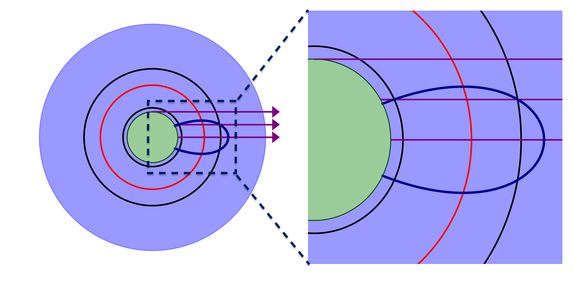
If $\Xi(y_{\infty}-1)<h<\Xi(y_{max})$, then the continuum ray will intersect $\Omega_{x}$ twice. Setting $\Xi=h$, we deduce the following relation,

$\displaystyle\frac{h^{2}}{(y_{\infty}-y)^{2/\gamma}}=1-\left(\frac{x}{y}\right)^{2},$

(7)

which has solutions $y_{h_{1}}$ and $y_{h_{2}}$ corresponding to the intrinsic velocities of the shells intersecting $\Gamma_{x}$ at height $h$. Shells with intrinsic velocities $y_{h_{1}}$ and $y_{h_{2}}$ for a fixed value of $h$ are shown in black in Figure 3. Finally, if $h<\Xi(y_{\infty}-1)$ the continuum ray will intersect $\Omega_{x}$ only once.

Putting it all together, we compute the absorption spectrum as follows. We define the integrand, $\rm{ABS}$, as

	$\displaystyle\rm{ABS}$	$\displaystyle=$	$\displaystyle 2\pi h(1-e^{-\bar{\tau}_{S}})|dh/dy|/\pi$
		$\displaystyle=$	$\frac{2}{\gamma}\left[\frac{x^{2}}{y^{2}}(y_{\infty}-y)^{\frac{2-\gamma}{\gamma}}+\frac{\gamma x^{2}}{y^{3}}(y_{\infty}-y)^{\frac{2}{\gamma}}-(y_{\infty}-y)^{\frac{2-\gamma}{\gamma}}\right]$
		$\displaystyle\times$	$\displaystyle(1-e^{-\bar{\tau}_{S}(y)}),$		(9)

where $\bar{\tau}_{S}(y)$ is defined over the following cases.

$$\displaystyle\bar{\tau}_{S}\equiv\begin{cases}\tau_{S}(y_{h_{1}})+\tau_{S}(y_{h_{2}})&\ \rm{if}\ \Xi(y_{\infty}-1)\leq\Xi(y)<\Xi(y_{\rm{max}})\\[10.00002pt] \tau_{S}(y)&\ \rm{otherwise}\\ \end{cases}$$

(10)

and $\tau_{S}$ is the Sobolev optical depth (Lamers & Cassinelli, 1999) defined as

$\displaystyle\tau_{S}$

$\displaystyle=$

$\displaystyle\frac{\pi e^{2}}{mc}f_{lu}\lambda_{lu}n_{l}(r)\left[1-\frac{n_{u}g_{l}}{n_{l}g_{u}}\right]\frac{r/v}{1+\sigma{\cos^{2}{\phi}}},$

(11)

where $f_{ul}$ and $\lambda_{ul}$ are the oscillator strength and wavelength, respectively, for the $ul$ transition, $\sigma=\frac{d\ln(v)}{d\ln(r)}-1$, and $\phi$ is the angle between the velocity and incoming photon ray (Castor, 1970). All other quantities take their usual definition. Writing Equation 11 in terms relevant to the SALT model, and by neglecting stimulated emission (i.e., $\left[1-\frac{n_{u}g_{l}}{n_{l}g_{u}}\right]=1$), we get

$\displaystyle\tau_{S}(y)=\tau_{0}\frac{(y_{\infty}-y)^{(1-\delta)/\gamma}}{y+[\gamma(y_{\infty}-y)-y](x/y)^{2}]},$

(12)

where

$\displaystyle\tau_{0}=\frac{\pi e^{2}}{mc}f_{lu}\lambda_{lu}n_{0}\frac{R_{SF}}{v_{0}}.$

(13)

Note that we are assuming that the population of the excited state is negligible ($n_{u}\sim 0$), and are therefore excluding the possibility of emission from the inflow and are focusing exclusively on continuum scattering. We will consider an emission component in a future paper and extend the range of our model to include radio observations and the interpretation of the inverse P Cygni profiles frequently observed in the spectra of cool atomic and molecular inflows (e.g., González-Alfonso et al. 2012; Falstad et al. 2015; Herrera-Camus et al 2020).

Finally, if $\Xi(y_{max})\leq 1$, then the normalized absorption profile becomes:

(14)

where $F(x)/F_{c}(x)$ is the flux at $x$ normalized by the continuum flux. If $\Xi(y_{max})>1$, then the normalized absorption profile becomes

$\displaystyle\frac{I_{\rm{abs,red}}}{I_{0}}=\frac{F(x)}{F_{c}(x)}-\frac{F(x)}{F_{c}(x)}\int_{x}^{y_{h}}\rm{ABS}(y)\ dy,$

(15)

where $y_{h}=\rm{min}(y_{h_{2}}(1),y_{h_{1}}(1))$, and $y_{h_{2}}(1)$ and $y_{h_{1}}(1)$ are the solutions of equation 7 for $h=1$.

We can compute the emission component of the inflowing SALT model using the same general procedure used in the outflowing case (see Carr et al. 2022, in prep). To this end, we think of $\Gamma_{x}(y)$ as a homotopy (i.e., a continuous map between surfaces of constant observed velocity), and compute the amount of energy absorbed by each surface that lies within the shell as we move in observed velocity space from $x=y\cos{\Theta_{C}}$ to $x=y$ where $\Theta_{C}=\arcsin{\left([y_{\infty}-y]^{-1/\gamma}\right)}$. Similar to the absorption case, we must be careful to identify which rays intersect $\Omega_{x}(y)$ before reaching the shell. With this in mind, we compute the total energy absorbed by a shell at velocity $y$ in the inflow as

	$\displaystyle L_{\rm{shell}}=$
			(16)

where $L(x)$ is the total energy emitted by the shell at resonance with material moving at observed velocity, $x$. We refer to SF as the Sobolev factor and define it for the following cases. If $y\geq y_{max}$, then

$\displaystyle\rm{SF}\equiv-[1-e^{-\tau_{S}(y)}];$

(17)

otherwise,

$\rm{SF}\equiv\begin{cases}e^{-\tau_{S}(y_{h_{2}})}[1-e^{-\tau_{S}(y_{h_{1}})}]&\ \rm{if}\ \Xi(y_{\infty}-1)\leq\Xi(y)<\Xi(y_{\rm{max}})\\[10.00002pt] 1-e^{-\tau_{S}(y)}&\ \rm{otherwise,}\\ \end{cases}$

(18)

where $\tau_{S}$ is given by Equation 12. The leading negative sign in Equation 17 accounts for the sign change in $dh$ when $y>y_{max}$. Now that we know the total energy absorbed by the shell, the reemission of energy in terms of the observed velocities can be computed exactly as in the outflowing case, albeit for a change in orientation (see Carr et al. 2022, in prep). We compute the normalized red emission profile as

	$\displaystyle I_{\rm{em,red}}/I_{0}=$
			(19)

where $SF$ is defined for the cases given above. Similar to the outflowing case, we account for the occultation effect on the blue emission profile by removing all photons reemitted from behind the source at heights $h=\Xi<1$. To this end, we define the scale factor $\Theta_{\rm{blue}}\equiv\Theta(\Xi-1)$ such that

$$\displaystyle\Theta\equiv\begin{cases}1&\rm{if\ }\ \Xi>1\\[10.00002pt] 0&\rm otherwise.\\ \end{cases}$$

(20)

The normalized blue emission profile becomes

	$\displaystyle I_{\rm{em,blue}}/I_{0}=$
			(21)

The technique developed by Carr et al. (2018) to account for the effects of a biconical outflow geometry still holds and can be applied to the line profile in the obvious way; however, rays which can interact with a surface of constant observed velocity more than once must be handled carefully since the geometry of the flow may be different at each interaction. When this is the case, we can approximate the expression for $SF$ in Equation 18 as

$\displaystyle f_{g}(y_{h_{1}})[I(y_{h_{2}})-I(y_{h_{2}})e^{-\tau_{S}(y_{h_{1}})}],$

(22)

where

$\displaystyle I=1-f_{g}(y_{h_{2}})[1-e^{-\tau_{S}(y_{h_{2}})}],$

(23)

and $f_{g}$ is the geometric factor as defined by Carr et al. (2018). Likewise, the Sobolev factor defined in Equations 9 & 10 will also need to change to the expression in Equation 22, but with the addition of the term, $f_{g}(y_{h_{2}})[1-e^{-\tau_{S}(y_{h_{2}})}]$. The techniques developed by Carr et al. (2018, 2021) to account for a dusty CGM, a limiting observing aperture, and holes in the outflow still hold and can be applied in the obvious way. Lastly, the multiple scattering procedure of Scarlata & Panagia (2015) used to account for resonant and fluorescent reemission still applies.

The absorption, emission, and full line profile or inverse P Cygni profile for a spherical inflow are shown in Figure 4. The most striking difference when compared to the traditional line profiles of outflows is that absorption now occurs to the right of systemic velocity or at positive observed velocities using our orientation. The emission profile is now more sharply peaked with a wider base compared to that of an outflow. This is because, in our model, the highest density material near the source is moving at the highest velocities - opposite of the outflowing case - thus the majority of energy is now spread over a larger observed velocity range; however, absorption (and reemission) can still occur in shells with low intrinsic velocities all the way to zero intrinsic velocity (outflows are cut off at the launch velocity) and accumulate emission into a sharp peak.

By far the most convincing evidence for inflows in absorption line studies is the direct detection of inverse P Cygni profiles (e.g., Rupke et al. 2021). These line profiles are characterized by having an overall net blueshift in emission and an overall net redshift in absorption. The latter of which is a stark quality unique to the spectra of inflowing gas; however, to declare the detection of an inflow, the redshifted absorption must reach observed velocities exceeding the limitations of the spectral resolution of the study. Furthermore, the absorption must be asymmetric with respect to line center (e.g., Martin et al. 2012) to distinguish the inflow from possible ISM absorption or thermal/turbulent line broadening (Carr et al. 2022, in prep). Here we investigate which parameter ranges favor detections of inflows in absorption for cases of pure spherical inflows and inflows with covering fractions less than unity.

We examine the effects of varying the power laws of both the density field (left column) and velocity field (right column) on the line profile of a spherical inflow in Figure 5. We have chosen to model the Fe II $2382$Å resonant transition which was used in the study by Martin et al. (2012) to identify inflows and outflows in galaxies at redshifts $0.4<z<1.4$ as an example. All atomic data for the lines used in this paper is provided in Table 2. In each column, we show how the absorption (top panel), emission (middle panel), and full inverse P Cygni profile (bottom panel) vary as functions of $\delta$ (left column) and $\gamma$ (right column) for fixed column density, $\log{(N\ [\rm{cm}^{-2}])}=15$. In regards to density, the amount of absorption at low observed velocities increases with decreasing $\delta$. This is because for steep density fields, most absorption is happening near the source at high observed velocities. When the density field becomes shallower, however, more absorption can occur at larger radii or at lower observed velocities. The spectrum varies significantly less over our chosen range for $\gamma$, but absorption does appear to increases at lower observed velocities for increasing $\gamma$. This occurs because the size of the inflow (i.e., $R_{W}=R_{SF}(v_{\infty}/v_{0})^{1/\gamma}$) increases with decreasing $\gamma$. Therefore, the bulk of material at low velocity is moving further away from the galaxy at lower density. We can conclude that steeper density and shallower velocity fields yield better conditions for identifying inflows. Under these conditions, most absorption will occur near the maximum observed velocity of the flow creating a more asymmetric (with regards to systemic velocity) absorption profile.

In Figure 6, we break the assumption of spherical symmetry and consider biconical inflows. These are the same geometrical models used by Carr et al. (2018), but are now inflowing. We mention that this is only an example, and note that the SALT model can just as easily be used in the case of a single cone geometry. In the left panel of Figure 6, we vary the opening angle, $\alpha$, of an inflow oriented along the line of sight. As is the case with outflows (see Carr et al. 2018), there is less reemission for smaller opening angles. This includes reducing the amount of red emission infilling²²2This is an analogous effect to the blue emission infilling which is typically associated with outflows., which enhances the increase of absorption for smaller opening angles. The opposite effect occurs when increasing the orientation angle, $\psi$, which is shown for an inflow with an opening angle $\alpha=30^{\circ}$ in the right panel of Figure 6. As $\psi$ increases, the inflowing gas is moved away from the line of sight, which results in less absorption since there is less material between the observer and the source. Coincidently, more and more emission appears near systemic or zero observed velocity, reflecting the position of the inflow with respect to the observer. The importance of this example is to demonstrate that when spherical symmetry is broken either the absorption or emission equivalent width can dominate based on the orientation of the inflow with respect to the observer. In regards to detecting inflows, a red shifted absorption profile is still a dead give away for inflowing gas; however, a pure emission profile could be mistaken for outflowing gas. The only difference between emission profiles that arise from outflows and inflows, is that, in the case of inflows, they are much more narrow peaked with wider bases³³3Emission profiles with wider bases and narrow peaks are also characteristic of outflows with decelerating velocity fields.. In this instance, fitting these lines with a single Gaussian - as is typically done in more traditional modeling techniques - may be difficult. More than likely fitting these emission lines would require two Gaussians (one for the narrow component near systemic velocity and the second for the wider base) and be misinterpreted as representing two kinematically distinct components. Thus the necessity to fit emission profiles with more than one Gaussian could be evidence for inflowing gas.

Realistically, both accretion and feedback occur simultaneously in galaxies - for example, during gas recycling when material expelled by the galaxy is returned via gravity. This is a fair assumption given the high detection rate of outflows and the necessity for inflows brought on by simulations. In fact, it has been suggested that the presence of outflows can mask inflows in spectral lines preventing the latter’s detection (e.g., Martin et al. 2012). This can foreseeably occur if the symmetric, with respect to line center, emission profile of an outflow fills in the weaker absorption feature of an inflow. Since numerical simulations show that outflows typically emerge in the direction perpendicular to the face of the disc while inflows move in the plane of the disc, orientation should also play a factor.

In this section, we attempt to explore which conditions favor the detection of inflows in galactic fountains (i.e., galactic systems with both inflows and outflows). To prevent the masking scenario mentioned above, we have chosen to model the Fe II 2343Å line. This line has two strong fluorescent channels at wavelengths 2365Å and 2381Å, and will therefore incur very little resonant emission (see Scarlata & Panagia 2015 for a detailed description of the role fluorescence plays in resonant scattering). In addition, ignoring the emission component will also allow us to much more easily model the simultaneous outflowing and inflowing of a single ionic species in SALT. In fact, under these conditions we can compute the spectrum from each model (inflow and outflow) independently and take the final spectrum as the superposition; otherwise, more modeling would be necessary to account for photons which are scattered by both the outflow and inflow. We also note that this situation can be enforced observationally by limiting the portion of the outflow captured by the observing aperture. By limiting the field of view to exclude the outflow except along the line of sight, one can effectively eliminate the entire emission component of a line profile (see Scarlata & Panagia 2015 for justification). This technique is feasible with IFU spectroscopy where one can obtain spectra from sub images.

We explore how the line profile of a galactic fountain changes with orientation in Figure 7. We show both a medium ($50\ \rm{km}\ \rm{s}^{-1}$) and a low ($120\ \rm{km}\ \rm{sec}^{-1}$) resolution spectra which has been smoothed with a Gaussian kernel. The latter is about the high resolution limit of the study by Martin et al. (2012). In this setup, we are assuming that the outflows and inflows occupy separate regions of the CGM with inflows moving perpendicular to a biconical outflow. Specifically, the models are made by generating the spectrum of a spherical inflow, removing the contribution of a biconical inflow from that spectrum, and then replacing it with a spectrum produced by a biconical outflow refilling that space. The remaining volume filled by inflowing gas is roughly the shape of a torus. Leaving such a large volume for the inflows represents a best case scenario for observing them. As expected, the orientation (compare the top two profiles) strongly affects our ability to detect an inflow at all resolutions: If there is no gas moving along the line of sight then we cannot detect any redshifted absorption, and thus have no possible way to identify an inflow given the weak emission component for this line. In the bottom panel, the low resolution spectrum of both the outflow and inflow appears to have merged together making it impossible to distinguish the inflow from another absorption feature such as absorption occurring in the ISM. This appears to be another form of masking by the outflow since this would not be the case if the outflow were absent (see the blue profile). There does appear to be hope of identifying the inflow at $50\ \rm{km}\ \rm{s}^{-1}$ resolution, however, since the asymmetric redshifted absorption feature becomes visible.

In the case of a true fountain, where warm ($5050\rm{K}<T<2\times 10^{4}\rm{K}$) ejected gas doesn’t have enough energy to escape the gravitational potential well, large regions of the CGM can have both an inflowing and outflowing component (see Kim & Ostriker 2018). We attempt to model such situations in Figure 8, where we show various outflows with an inflowing gas component occupying the same general volume. For each scenario, we have chosen covering fractions for the outflows, $f_{c,o}$, and inflows, $f_{c,i}$, such that $f_{c,o}+f_{c,i}=1$ and $f_{c,i}<f_{c,o}$ with the order representing the fact that inflows are typically expected to have smaller covering fractions than outflows (Kimm et al., 2011). Once again, we are not able to identify inflows at the $120\ \rm{km}\ \rm{sec}^{-1}$ resolution level given our model constraints, but are able to at the $50\ \rm{km}\ \rm{s}^{-1}$ level. This strongly suggests that the number of inflows detected in large low resolution surveys is undercounted, and can be improved by moving to higher, but still obtainable resolutions by active instruments.

References

- Anglés-Alcázar et al. (2017) Anglés-Alcázar, D., Faucher-Giguère, C.-A., Kereš, D., et al. 2017, MNRAS, 470, 4698. doi:10.1093/mnras/stx1517
- Carr et al. (2018) Carr, C., Scarlata, C., Panagia, N., & Henry, A. 2018, ApJ, 860, 143
- Carr et al. (2021) Carr, C., Scarlata, C., Henry, A., et al. 2021, ApJ, 906, 104. doi:10.3847/1538-4357/abc7c3
- Castor (1970) Castor, J. I. 1970, MNRAS, 149, 111. doi:10.1093/mnras/149.2.111
- Chisholm et al. (2016) Chisholm, J., Tremonti Christy, A., Leitherer, C., et al. 2016, MNRAS, 463, 541. doi:10.1093/mnras/stw1951
- Chisholm et al. (2017a) Chisholm, J., Orlitová, I., Schaerer, D., et al. 2017, A&A, 605, A67. doi:10.1051/0004-6361/201730610
- Chisholm et al. (2017b) Chisholm, J., Tremonti, C. A., Leitherer, C., et al. 2017, MNRAS, 469, 4831. doi:10.1093/mnras/stx1164
- Erb (2008) Erb, D. K. 2008, ApJ, 674, 151. doi:10.1086/524727
- Falstad et al. (2015) Falstad, N., González-Alfonso, E., Aalto, S., et al. 2015, A&A, 580, A52
- Faucher-Giguère (2017) Faucher-Giguère, C.-A. 2017, Gas Accretion onto Galaxies, 271. doi:10.1007/978-3-319-52512-9_12
- Fielding & Bryan (2022) Fielding, D. B. & Bryan, G. L. 2022, ApJ, 924, 82. doi:10.3847/1538-4357/ac2f41
- Ford et al. (2014) Ford A. B., Dave R., Oppenheimer B. D., Katz N., Kollmeier J. A., Thompson R., Weinberg D. H., 2014, MNRAS, 444, 1260 (F14)
- Gallerani et al. (2018) Gallerani, S., Pallottini, A., Feruglio, C., et al. 2018, MNRAS, 473, 1909. doi:10.1093/mnras/stx2458
- Gazagnes et al. (2018) Gazagnes, S., Chisholm, J., Schaerer, D., et al. 2018, A&A, 616, A29. doi:10.1051/0004-6361/201832759
- González-Alfonso et al. (2012) Gonzalez-Alfonso, E., Fischer, J., Gracia-Carpio, J., et al. 2012, A&A, 541, 4
- Heckman et al. (2017) Heckman, T., Borthakur, S., Wild, V., et al. 2017, ApJ, 846, 151. doi:10.3847/1538-4357/aa80dc
- Herrera-Camus et al (2020) Herrera-Camus, R., Sturm, E., Graciá-Carpio, J., et al. 2020, A&A, 633, L4
- Ho & Martin (2020) Ho, S. H. & Martin, C. L. 2020, ApJ, 888, 14. doi:10.3847/1538-4357/ab58cd
- Hopkins et al. (2014) Hopkins, P. F., Kereš, D., Oñorbe, J., et al. 2014, MNRAS, 445, 581. doi:10.1093/mnras/stu1738
- Hopkins et al. (2018) Hopkins, P. F., Wetzel, A., Kereš, D., et al. 2018, MNRAS, 480, 800. doi:10.1093/mnras/sty1690
- Kim & Ostriker (2018) Kim, C.-G. & Ostriker, E. C. 2018, ApJ, 853, 173. doi:10.3847/1538-4357/aaa5ff
- Kimm et al. (2011) Kimm, T., Slyz, A., Devriendt, J., et al. 2011, MNRAS, 413, L51. doi:10.1111/j.1745-3933.2011.01031.x
- Laha et al. (2018) Laha, S., Guainazzi, M., Piconcelli, E., et al. 2018, ApJ, 868, 10. doi:10.3847/1538-4357/aae390
- Lamers & Cassinelli (1999) Lamers, H. J. G. L. M. & Cassinelli, J. P. 1999, Introduction to Stellar Winds, 452
- Martin et al. (2012) Martin, C. L., Shapley, A. E., Coil, A. L., et al. 2012, ApJ, 760, 127
- Mannucci et al. (2010) Mannucci, F., Cresci, G., Maiolino, R., et al. 2010, MNRAS, 408, 2115. doi:10.1111/j.1365-2966.2010.17291.x
- Oppenheimer & Davé (2006) Oppenheimer, B. D. & Davé, R. 2006, MNRAS, 373, 1265. doi:10.1111/j.1365-2966.2006.10989.x
- Papovich et al. (2011) Papovich, C., Finkelstein, S. L., Ferguson, H. C., et al. 2011, MNRAS, 412, 1123. doi:10.1111/j.1365-2966.2010.17965.x
- Peeples et al. (2014) Peeples, M. S., Werk, J. K., Tumlinson, J., et al. 2014, ApJ, 786, 54. doi:10.1088/0004-637X/786/1/54
-
Prochaska et al. (2011)
Prochaska, J. X., Kasen, D., & Rubin, K. 2011, ApJ, 734, 24. doi:10.1088/0004-637X/734/1/24
- Rivera-Thorsen et al. (2015) Rivera-Thorsen, T. E., Hayes, M., Östlin, G., et al. 2015, ApJ, 805, 14. doi:10.1088/0004-637X/805/1/14
- Roberts-Borsani & Saintonge (2019) Roberts-Borsani, G. W. & Saintonge, A. 2019, MNRAS, 482, 4111. doi:10.1093/mnras/sty2824
- Rubin et al. (2012) Rubin, K. H. R., Prochaska, J. X., Koo, D. C., et al. 2012, ApJ, 747, L26. doi:10.1088/2041-8205/747/2/L26
- Rubin et al. (2014) Rubin, K. H. R., Prochaska, J. X., Koo, D. C., et al. 2014, ApJ, 794, 156. doi:10.1088/0004-637X/794/2/156
- Rupke et al. (2021) Rupke, D. S. N., Thomas, A. D., & Dopita, M. A. 2021, MNRAS, 503, 4748. doi:10.1093/mnras/stab743
- Scarlata & Panagia (2015) Scarlata, C, and Panagia, N. ”A semi-analytical line transfer model to interpret the spectra of galaxy outflows.” The Astrophysical Journal 801, no. 1 (2015): 43.
- Somerville & Davé (2015) Somerville, R. S., & Davé, R. 2015, ARA&A, 53, 51
- Springel (2005) Springel, V. 2005, MNRAS, 364, 1105. doi:10.1111/j.1365-2966.2005.09655.x
- Stocke et al. (2013) Stocke, J. T., Keeney, B. A., Danforth, C. W., et al. 2013, ApJ, 763, 148. doi:10.1088/0004-637X/763/2/148
Strickland et al. (1997)
Strickland, D. K., Ponman, T. J., & Stevens, I. R. 1997, A&A, 320, 378
- Tumlinson et al. (2017) Tumlinson, J., Peeples, M. S., & Werk, J. K. 2017, ARA&A, 55, 389. doi:10.1146/annurev-astro-091916-055240
- Veilleux et al. (2020) Veilleux, S., Maiolino, R., Bolatto, A. D., et al. 2020, A&A Rev., 28, 2. doi:10.1007/s00159-019-0121-9
- Vogelsberger et al. (2014) Vogelsberger, M., Genel, S., Springel, V., et al. 2014, MNRAS, 444, 1518. doi:10.1093/mnras/stu1536
- Werk et al. (2014) Werk J. K. et al., 2014, ApJ, 792, 8
- Xu et al. (2022) Xu, X., Heckman, T., Henry, A., et al. 2022, arXiv:2204.09181
- Zhu et al. (2015) Zhu, G. B., Comparat, J., Kneib, J.-P., et al. 2015, ApJ, 815, 48. doi:10.1088/0004-637X/815/1/48