A search for relativistic ejecta in a sample of ZTF broad-lined Type Ic supernovae
Abstract
The dividing line between gamma-ray bursts (GRBs) and ordinary stripped-envelope core-collapse supernovae (SNe) is yet to be fully understood. Observationally mapping the variety of ejecta outcomes (ultra-relativistic, mildly-relativistic or non-relativistic) in SNe of Type Ic with broad lines (Ic-BL) can provide a key test to stellar explosion models. However, this requires large samples of the rare Ic-BL events with follow-up observations in the radio, where fast ejecta can be probed largely free of geometry and viewing angle effects. Here, we present the results of a radio (and X-ray) follow-up campaign of 16 SNe Ic-BL detected by the Zwicky Transient Facility (ZTF). Our radio campaign resulted in 4 counterpart detections and 12 deep upper limits. None of the events in our sample is as relativistic as SN 1998bw and we constrain the fraction of SN 1998bw-like explosions to (3 Gaussian equivalent), a factor of smaller than previously established. We exclude relativistic ejecta with radio luminosity densities in between erg s-1 Hz-1 and erg s-1 Hz-1 at d since explosion for of the events in our sample. This shows that SNe Ic-BL similar to the GRB-associated SN 1998bw, SN 2003lw, SN 2010dh, or to the relativistic SN 2009bb and iPTF17cw, are rare. Our results also exclude an association of the SNe Ic-BL in our sample with largely off-axis GRBs with energies erg. The parameter space of SN 2006aj-like events (faint and fast-peaking radio emission) is, on the other hand, left largely unconstrained and systematically exploring it represents a promising line of future research.
1 Introduction
Massive stars contribute to the chemical composition of matter as we know it in the universe, and their deaths are accompanied by energetic core-collapse supernovae (SNe) that seed our universe with black holes (BHs) and neutron stars (NSs) – the most exotic objects of the stellar graveyard. Large time-domain surveys of the sky (e.g., York et al., 2000; Drake et al., 2009; Law et al., 2009; Kaiser et al., 2010; Shappee et al., 2014; Dark Energy Survey Collaboration et al., 2016; Tonry et al., 2018d; Bellm et al., 2019), paired with targeted follow-up efforts, have greatly enriched our view on the final stages of massive star evolution. Yet, a lot remains to be understood about the diverse paths that bring massive stars toward their violent deaths (Langer, 2012).
Core-collapse SNe can occur in stars with a hydrogen envelope (Type II) or in stars where hydrogen is almost or completely missing (Type Ib/c, also referred to as stripped-envelope SNe; Filippenko, 1997; Matheson et al., 2001; Li et al., 2011; Modjaz et al., 2014; Perley et al., 2020; Frohmaier et al., 2021). Type Ib/c SNe constitute approximately 25% of all massive star explosions (Smith et al., 2011), and their pre-SN progenitors are thought to be either massive ( M⊙) and metal-rich single stars that have been stripped through stellar mass loss; or the mass donors in close binary systems (at any metallicity) that have initial masses M⊙ (e.g., Langer, 2012, and references therein).
A small fraction of Type Ib/c SNe show velocities in their optical spectra that are systematically higher than those measured in ordinary SNe Ic at similar epochs. Hence, these explosions are referred to as SNe of Type Ic with broad lines (hereafter, Ic-BL; e.g., Filippenko, 1997; Modjaz et al., 2016; Gal-Yam, 2017). Compared to Type Ib/c SNe, broad-lined events are found to prefer environments with lower metallicity (in a single star scenario, mass loss mechanisms also remove angular momentum and are enhanced by higher metallicities), and in galaxies with higher star-formation rate density. Thus, it has been suggested that SN Ic-BL progenitors may be stars younger and more massive than those of normal Type Ic (more massive progenitors can lose their He-rich layers to winds at lower metallicity due to the higher luminosities driving the winds), and/or tight massive binary systems that can form efficiently in dense stellar clusters (e.g., Kelly et al., 2014; Japelj et al., 2018; Modjaz et al., 2020).
The spectroscopic and photometric properties used to classify core-collapse SNe are largely determined by the stars’ outer envelopes (envelope mass, radius, and chemical composition; Young, 2004). On the other hand, quantities such as explosion energies, nickel masses, and ejecta geometries can be inferred via extensive multi-wavelength and multi-band observations. These quantities, in turn, can help constrain the properties of the stellar cores (such as mass, density structure, spin, and magnetic fields; see e.g. Woosley et al., 2002; Burrows et al., 2007; Jerkstrand et al., 2015, and references therein) that are key to determine the nature of the explosion. For example, based on nickel masses and ejecta masses derived from bolometric light curve analyses, Taddia et al. (2019) found that of Ic-BL progenitors are compatible with massive ( M⊙), possibly single stars, whereas could be associated with less massive stars in close binary systems.
Understanding the progenitor scenario of SNe Ic-BL is particularly important as these SNe challenge greatly the standard explosion mechanism of massive stars (e.g., Mezzacappa et al., 1998; MacFadyen & Woosley, 1999; Heger et al., 2003; Woosley & Heger, 2006; Janka et al., 2007; Janka, 2012; Smith, 2014; Foglizzo et al., 2015; Müller, 2020; Schneider et al., 2021, and references therein). The energies inferred from optical spectroscopic modeling of Ic-BL events are of order , in excess of the inferred in typical SNe Ib/c, while ejecta masses are comparable or somewhat higher (Taddia et al., 2019). In the traditional core-collapse scenario, neutrino irradiation from the proto-NS revives the core-bounce shock, making the star explode. However, the neutrino mechanism cannot explain the more energetic SNe Ic-BL. Unveiling the nature of an engine powerful enough to account for the extreme energetics of SNe Ic-BL is key to understanding the physics behind massive stellar deaths, and remains as of today an open question.
A compelling scenario invokes the existence of a jet or a newly-born magnetar as the extra source of energy needed to explain SNe Ic-BL (e.g., Burrows et al., 2007; Papish & Soker, 2011; Gilkis & Soker, 2014; Mazzali et al., 2014; Lazzati et al., 2012; Gilkis et al., 2016; Soker & Gilkis, 2017; Barnes et al., 2018; Shankar et al., 2021). The rapid rotation of a millisecond proto-NS formed in the collapse of a rotating massive star can amplify the NS magnetic field to G, creating a magnetar. The magnetar spins down quickly via magnetic braking, and in some cases magneto-rotational instabilities can launch a collimated jet that drills through the outer layers of the star producing a gamma-ray burst (GRB; e.g., Heger et al., 2003; Izzard et al., 2004; Woosley & Heger, 2006; Burrows et al., 2007; Bugli et al., 2020, 2021). These jets can transfer sufficient energy to the surrounding stellar material to explode it into a SN.
The above scenario is particularly interesting in light of the fact that SNe Ic-BL are also the only type of core-collapse events that, observationally, have been unambiguously linked to GRBs (e.g., Woosley & Bloom, 2006; Cano et al., 2017, and references therein). GRBs are characterized by bright afterglows that emit radiation from radio to X-rays, and are unique laboratories for studying relativistic particle acceleration and magnetic field amplification processes (Piran, 2004; Mészáros, 2006). In between ordinary SNe Ic-BL and cosmological GRBs is a variety of transients that we still have to fully characterize. Among those are low-luminosity GRBs, of which the most famous example is GRB 980425, associated with the radio-bright Type Ic-BL SN 1998bw (Galama et al., 1998; Kulkarni et al., 1998).
Recently, Shankar et al. (2021) used the jetted outflow model produced from a consistently formed proto-magnetar in a 3D core-collapse SN to extract a range of central engine parameters (energy and opening angle ) that were then used as inputs to hydrodynamic models of jet-driven explosions. The output of these models, in turn, were used to derive predicted SN light curves and spectra from different viewing angles, and found to be in agreement with SN Ic-BL optical observables (see also Barnes et al., 2018). It was also shown that additional energy from the engine can escape through the tunnel drilled in the star as an ultra-relativistic jet (GRB) with energy erg. On the other hand, a SN Ic-BL can be triggered even if the jet engine fails to produce a successful GRB jet. The duration of the central engine, , together with and , are critical to determining the fate of the jet (Lazzati et al., 2012).
A more general scenario where the high velocity ejecta found in SNe Ic-BL originate from a cocoon driven by a relativistic jet (regardless of the nature of the central engine) is also receiving attention. In this scenario, cosmological long GRBs are explosions where the relativistic jet breaks out successfully from the stellar envelope, while low-luminosity GRBs and SNe Ic-BL that are not associated with GRBs represent cases where the jet is choked (see e.g. Piran et al., 2019; Eisenberg et al., 2022; Gottlieb et al., 2022; Pais et al., 2022, and references therein).
Overall, the dividing line between successful GRB jets and failed ones is yet to be fully explored observationally, and observed jet outcomes in SNe Ic-BL have not yet been systematically compared to model outputs. While we know that SNe discovered by means of a GRB are all of Type Ic-BL, the question that remains open is whether all SNe Ic-BL make a GRB (jet), at least from some viewing angle, or if instead the jet-powered SNe Ic-BL are intrinsically different and rarer than ordinary SNe Ic-BL. Indeed, due to the collimation of GRB jets, it is challenging to understand whether all SNe Ic-BL are linked to successful GRBs: a non-detection in - or X-rays could simply be due to the explosion being directed away from us. Radio follow-up observations are needed to probe the explosions’ fastest-moving ejecta () largely free of geometry and viewing angle constraints. Determining observationally what is the fraction of Type Ic-BL explosions that output jets which successfully break out of the star (as mildly-relativistic or ultra-relativistic ejecta), and measuring their kinetic energy via radio calorimetry, can provide jet-engine explosion models a direct test of their predictions.
Using one of the largest sample of SNe Ic-BL with deep radio follow-up observations (which included 15 SNe Ic-BL discovered by the Palomar Transient Factory, PTF/iPTF; Law et al., 2009), Corsi et al. (2016) already established that of SNe Ic-BL harbor relativistic ejecta similar to that of SN 1998bw. Here, we present the results of a systematic radio follow-up campaign of an additional 16 SNe Ic-BL (at ) detected independently of -rays by the Zwicky Transient Facility (ZTF; Bellm et al., 2019; Graham et al., 2019). This study greatly expands our previous works on the subject (Corsi et al., 2017, 2016, 2014). Before the advent of PTF and ZTF, the comparison between jet-engine model outcomes and radio observables was severely limited by the rarity of SN Ic-BL discoveries (e.g., Berger et al., 2003; Soderberg et al., 2006a) and/or by selection effects (e.g., Woosley & Bloom, 2006)—out of the thousands of jets identified, nearly all were discovered at large distances via their high-energy emission (implying aligned jet geometry and ultra-relativistic speeds). In this work, we aim to provide a study free of these biases.
Our paper is organized as follows. In Section 2 we describe our multi-wavelength observations; in Section 3 we describe in more details the SNe Ic-BL included in our sample; in Section 4 we model the optical, X-ray, and radio properties of the SNe presented here and derive constraints on their progenitor and ejecta properties. Finally, in Section 5 we summarize and conclude. Hereafter we assume cosmological parameters km s-1 Mpc-1, , (Bennett et al., 2014). All times are given in UT unless otherwise stated.
| SN (ZTF name) | RA, Dec (J2000) | ||
|---|---|---|---|
| (hh:mm:ss dd:mm:ss) | (Mpc) | ||
| 2018etk (18abklarx) | 15:17:02.53 +03:56:38.7 | 0.044 | 196 |
| 2018hom (18acbwxcc) | 22:59:22.96 +08:45:04.6 | 0.030 | 132 |
| 2018hxo (18acaimrb) | 21:09:05.80 +14:32:27.8 | 0.048 | 214 |
| 2018jex (18acpeekw) | 11:54:13.87 +20:44:02.4 | 0.094 | 434 |
| 2019hsx (19aawqcgy) | 18:12:56.22 +68:21:45.2 | 0.021 | 92 |
| 2019xcc (19adaiomg) | 11:01:12.39 +16:43:29.1 | 0.029 | 128 |
| 2020jqm (20aazkjfv) | 13:49:18.57 03:46:10.4 | 0.037 | 164 |
| 2020lao (20abbplei) | 17:06:54.61 +30:16:17.3 | 0.031 | 137 |
| 2020rph (20abswdbg) | 03:15:17.83 +37:00:50.8 | 0.042 | 187 |
| 2020tkx (20abzoeiw) | 18:40:09.01 +34:06:59.5 | 0.027 | 119 |
| 2021xv (21aadatfg) | 16:07:32.82 +36:46:46.2 | 0.041 | 182 |
| 2021aug (21aafnunh) | 01:14:04.81 +19:25:04.7 | 0.041 | 182 |
| 2021epp (21aaocrlm) | 08:10:55.27 06:02:49.3 | 0.038 | 168 |
| 2021htb (21aardvol) | 07:45:31.19 +46:40:01.3 | 0.035 | 155 |
| 2021hyz (21aartgiv) | 09:27:36.51 +04:27:11.0 | 0.046 | 205 |
| 2021ywf (21acbnfos) | 05:14:10.99 +01:52:52.4 | 0.028 | 123 |


2 Multi-wavelength observations
We have collected a sample of 16 SNe Ic-BL observed with the ZTF and with follow-up observations in the radio. The SNe Ic-BL included in our sample are listed in Table 1. We selected these SNe largely based on the opportunistic availability of follow-up observing time on the Karl G. Jansky Very Large Array (VLA). The sample of SNe presented here doubles the sample of SNe Ic-BL with deep VLA observations presented in Corsi et al. (2016).
The SNe considered in this work are generally closer than the PTF/iPTF sample of SNe Ic-BL presented in Taddia et al. (2019). In fact, their median redshift () is about twice as small as the median redshift of the PTF/iPTF SN Ic-BL sample (; Taddia et al., 2019). However, the median redshift of the ZTF SNe in our sample is compatible with the median redshift () of the full ZTF SN Ic-BL population presented in Srinivasaragavan et al. (2022). A subset of the SNe Ic-BL presented here is also analyzed in a separate paper and in a different context (r-process nucleosynthesis; Anand et al., 2022). In this work, we report for the first time the results of our radio follow-up campaign of these events. We note that the “Asteroid Terrestrial-impact Last Alert System”(ATLAS; Tonry et al., 2018d) has contributed to several of the SN detections considered here (see Section 3). Three of the Ic-BL in our sample were also reported in the recently released bright SN catalog by the All-Sky Automated Survey for Supernovae (ASAS-SN; Neumann et al., 2022).
In what follows, we describe the observations we carried for this work. In Section 3 we give more details on each of the SNe Ic-BL in our sample.
2.1 ZTF photometry
All photometric observations presented in this work were conducted with the Palomar Schmidt 48-inch (P48) Samuel Oschin telescope as part of the ZTF survey (Bellm et al., 2019; Graham et al., 2019), using the ZTF camera (Dekany et al., 2020). In default observing mode, ZTF uses 30 s exposures, and survey observations are carried out in and band, down to a typical limiting magnitude of mag. P48 light curves were derived using the ZTF pipeline (Masci et al., 2019), and forced photometry (see Yao et al., 2019). Hereafter, all reported magnitudes are in the AB system. The P48 light curves are shown in Figures 1-2. All the light curves presented in this work will be made public on the Weizmann Interactive Supernova Data Repository (WISeREP111https://www.wiserep.org/).
| SN | TXRT | Exp. | |
| (MJD) | (ks) | ( erg cm-2 s-1) | |
| 2018etk | 58377.85 | 4.8 | |
| 2018hom | 58426.02 | 4.3 | |
| 2019hsx | 58684.15 | 15 | |
| 2020jqm | 59002.09 | 7.4 | |
| 2020lao | 59007.40 | 14 | |
| 2020rph | 59088.89 | 7.5 | |
| 2020tkx | 59125.38 | 8.1 | |
| 2021hyz | 59373.09 | 4.7 | |
| 2021ywf | 59487.60 | 7.2 |
2.2 Optical Spectroscopy
Preliminary spectral type classifications of several of the SNe in our sample were obtained with the Spectral Energy Distribution Machine (SEDM) mounted on the Palomar 60-inch telescope (P60), and quickly reported to the Transient Name Server (TNS). The SEDM is a very low resolution () integral field unit spectrograph optimized for transient classification with high observing efficiency (Blagorodnova et al., 2018; Rigault et al., 2019).
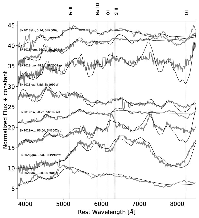
After initial classification, typically further spectroscopic observations are carried out as part of the ZTF transient follow-up programs to confirm and/or improve classification, and to characterize the time-evolving spectral properties of interesting events. Amongst the series of spectra obtained for each of the SNe presented in this work, we select one good quality photospheric phase spectrum (Figures 3-4; grey) on which we run SNID (Blondin & Tonry, 2007) to obtain the best match to a SN Ic-BL template (black), after clipping the host emission lines and fixing the redshift to that derived either from the SDSS host galaxy or from spectral line fitting (H; see Section 3 for further details). Hence, in addition to the SEDM, in this work we also made use of the following instruments: the Double Spectrograph (DBSP; Oke et al., 1995), a low-to-medium resolution grating instrument for the Palomar 200-inch telescope Cassegrain focus that uses a dichroic to split light into separate red and blue channels observed simultaneously; the Low Resolution Imaging Spectrometer (LRIS; Oke & Gunn, 1982; Oke et al., 1995), a visible-wavelength imaging and spectroscopy instrument operating at the Cassegrain focus of Keck-I; the Alhambra Faint Object Spectrograph and Camera (ALFOSC), a CCD camera and spectrograph installed at the Nordic Optical Telescope (NOT; Djupvik & Andersen, 2010). All spectra presented in this work will be made public on WISeREP.
2.3 X-ray follow up with Swift
For 9 of the 16 SNe presented in this work we carried out follow-up observations in the X-rays using the X-Ray Telescope (XRT; Burrows et al., 2005) on the Neil Gehrels Swift Observatory (Gehrels et al., 2004).
We analyzed these observations using the online XRT tools222See https://www.swift.ac.uk/user_objects/., as described in Evans et al. (2009). We correct for Galactic absorption, and adopt a power-law spectrum with photon index for count rate to flux conversion for non-detections, and for detections (two out of ninw events) where the number of photons collected is too small to enable a meaningful spectral fit (one out of two detections). Table 2 presents the results from co-adding all observations of each source.
2.4 Radio follow up with the VLA
We observed the fields of the SNe Ic-BL in our sample with the VLA via several of our programs using various array configurations and receiver settings (Table LABEL:tab:data).
The VLA raw data were calibrated in CASA (McMullin et al., 2007) using the automated VLA calibration pipeline. After manual inspection for further flagging, the calibrated data were imaged using the tclean task. Peak fluxes were measured from the cleaned images using imstat and circular regions centered on the optical positions of the SNe, with radius equal to the nominal width (FWHM) of the VLA synthesized beam (see Table LABEL:tab:data). The RMS noise values were estimated with imstat from the residual images. Errors on the measured peak flux densities in Table LABEL:tab:data are calculated adding a 5% error in quadrature to measured RMS values. This accounts for systematic uncertainties on the absolute flux calibration.
We checked all of our detections (peak flux density above ) for the source morphology (extended versus point-like), and ratio between integrated and peak fluxes using the CASA task imfit. All sources for which these checks provided evidence for extended or marginally resolved emission are marked accordingly in Table LABEL:tab:data. For non detections, upper-limits on the radio flux densities are given at the level unless otherwise noted.
| SN | a | Conf. | Nom.Syn.Beam | Project | ||
| (MJD) | (GHz) | (Jy) | (FWHM; arcsec) | |||
| 2018etk | 58363.08 | 6.3 | b | D | 12 | VLA/18A-176d |
| 58374.09 | 14 | D | 4.6 | VLA/18A-176d | ||
| 58375.03 | 6.3 | b | D | VLA/18A-176d | ||
| 59362.27 | 6.2 | b | D | 12 | VLA/20B-149d | |
| 2018hom | 58428.04 | 6.6 | D | 12 | VLA/18A-176d | |
| 2018hxo | 58484.73 | 6.4 | c | C | 3.5 | VLA/18A-176d |
| 2018jex | 58479.38 | 6.4 | C | 3.5 | VLA/18A-176d | |
| 2019hsx | 58671.14 | 6.2 | BnA | 1.0 | VLA/19B-230d | |
| 2019xcc | 58841.43 | 6.3 | b | D | 12 | VLA/19B-230d |
| 58876.28 | 6.3 | b | D | 12 | VLA/19B-230d | |
| 59363.00 | 6.3 | b | D | 12 | VLA/20B-149d | |
| 2020jqm | 58997.03 | 5.6 | C | 3.5 | SG0117d | |
| 59004.03 | 5.6 | C | 3.5 | SG0117d | ||
| 59028.48 | 5.5 | B | 1.0 | VLA/20A-568d | ||
| 59042.95 | 5.7 | B | 1.0 | VLA/20A-568d | ||
| 59066.09 | 5.5 | B | 1.0 | VLA/20A-568d | ||
| 59088.03 | 5.5 | B | 1.0 | VLA/20A-568d | ||
| 59114.74 | 5.5 | B | 1.0 | VLA/20A-568d | ||
| 59240.37 | 5.5 | A | 0.33 | VLA/20B-149d | ||
| 2020lao | 59006.21 | 5.2 | C | 3.5 | SG0117d | |
| 59138.83 | 5.5 | B | 1.0 | SG0117d | ||
| 2020rph | 59089.59 | 5.5 | B | 1.0 | SG0117d | |
| 59201.28 | 5.5 | A | 0.33 | SG0117d | ||
| 2020tkx | 59117.89 | 10 | B | 0.6 | VLA/20A-374e | |
| 59136.11 | 10 | B | 0.6 | VLA/20A-374e | ||
| 59206.92 | 5.5 | A | 0.33 | VLA/20B-149d | ||
| 2021xv | 59242.42 | 5.5 | A | 0.33 | VLA/20B-149d | |
| 59303.24 | 5.2 | D | 12 | VLA/20B-149d | ||
| 59353.11 | 5.2 | b | D | 12 | VLA/20B-149d | |
| 2021aug | 59254.75 | 5.2 | A | 0.33 | VLA/20B-149d | |
| 59303.62 | 5.4 | D | 12 | VLA/20B-149d | ||
| 59353.48 | 5.4 | D | 12 | VLA/20B-149d | ||
| 2021epp | 59297.06 | 5.3 | b | D | 12 | VLA/20B-149d |
| 59302.99 | 5.1 | b | D | 12 | VLA/20B-149d | |
| 59352.83 | 5.3 | b | D | 12 | VLA/20B-149d | |
| 2021htb | 59324.94 | 5.2 | b | D | 12 | VLA/20B-149d |
| 59352.87 | 5.2 | b | D | 12 | VLA/20B-149d | |
| 2021hyz | 59326.08 | 5.2 | D | 12 | VLA/20B-149d | |
| 59352.99 | 5.5 | D | 12 | VLA/20B-149d | ||
| 2021ywf | 59487.57 | 5.0 | B | 1.0 | SH0105d | |
| 59646.12 | 5.4 | A | 0.33 | SH0105d | ||
| a Mid MJD time of VLA observation (total time including calibration). | ||||||
| b Resolved or marginally resolved with emission likely dominated by the host galaxy. | ||||||
| c Image is dynamic range limited due to the presence of a bright source in the field. | ||||||
| d PI: Corsi. | ||||||
| e PI: Ho. | ||||||

3 Sample description
3.1 SN 2018etk
Our first ZTF photometry of SN 2018etk (ZTF18abklarx) was obtained on 2018 August 1 (MJD 58331.16) with the P48. This first ZTF detection was in the band, with a host-subtracted magnitude of mag (Figure 1), at =15h17m02.53s, (J2000). The object was reported to the TNS by ATLAS on 2018 August 8, who discovered it on 2018 August 6 (Tonry et al., 2018a). The last ZTF non-detection prior to ZTF discovery was on 2018 July 16, and the last shallow ATLAS non-detection was on 2018 August 2, at mag. The transient was classified as a Type Ic SN by Fremling et al. (2018a) based on a spectrum obtained on 2018 August 13 with the SEDM. We re-classify this transient as a SN Type Ic-BL most similar to SN 2006aj based on a P200 DBSP spectrum obtained on 2018 August 21 (see Figure 3). SN 2018etk exploded in a star-forming galaxy with a known redshift of derived from SDSS data.
3.2 SN 2018hom
Our first ZTF photometry of SN 2018hom (ZTF18acbwxcc) was obtained on 2018 November 1 (MJD 58423.54) with the P48. This first ZTF detection was in the band, with a host-subtracted magnitude of mag (Figure 1), at =22h59m22.96s, (J2000). The object was reported to the TNS by ATLAS on 2018 October 26, and discovered by ATLAS on 2018 October 24 at mag (Tonry et al., 2018b). The last ZTF non-detection prior to ZTF discovery was on 2018 October 9 at mag, and the last ATLAS non-detection was on 2018 October 22 at mag. The transient was classified as a SN Type Ic-BL by Fremling et al. (2018b) based on a spectrum obtained on 2018 November 2 with the SEDM. SN 2018etk exploded in a galaxy with unknown redshift. We measure a redshift of from star-forming emission lines in a Keck-I LRIS spectrum obtained on 2018 November 30. We plot this spectrum in Figure 3, along with its SNID template match to the Type Ic-BL SN 1997ef. We note that this SN was also reported in the recently released ASAS-SN bright SN catalog (Neumann et al., 2022).
3.3 SN 2018hxo
Our first ZTF photometry of SN 2018hxo (ZTF18acaimrb) was obtained on 2018 October 9 (MJD 58400.14) with the P48. This first detection was in the band, with a host-subtracted magnitude of mag (Figure 1), at =21h09m05.80s, (J2000). The object was first reported to the TNS by ATLAS on 2018 November 6, and first detected by ATLAS on 2018 September 25 at mag (Tonry et al., 2018c). The last ZTF non-detection prior to discovery was on 2018 September 27 at mag, and the last ATLAS non-detection was on 2018 September 24 at mag. The transient was classified as a SN Type Ic-BL by Dahiwale & Fremling (2020a) based on a spectrum obtained on 2018 December 1 with Keck-I LRIS. In Figure 3 we plot this spectrum along with its SNID match to the Type Ic-BL SN 2002ap. SN 2018etk exploded in a galaxy with unknown redshift. We measure a redshift of from star-forming emission lines in the Keck spectrum.
3.4 SN 2018jex
Our first ZTF photometry of SN 2018jex (ZTF18acpeekw) was obtained on 2018 November 16 (MJD 58438.56) with the P48. This first detection was in the band, with a host-subtracted magnitude of mag, at =11h54m13.87s, (J2000). The object was reported to the TNS by AMPEL on November 28 (Nordin et al., 2018). The last ZTF last non-detection prior to ZTF discovery was on 2018 November 16 at mag. The transient was classified as a SN Type Ic-BL based on a spectrum obtained on 2018 December 4 with Keck-I LRIS. In Figure 3 we show this spectrum plotted against the SNID template of the Type Ic-BL SN 1997ef. AT2018jex exploded in a galaxy with unknown redshift. We measure a redshift of from star-forming emission lines in the Keck spectrum.
3.5 SN 2019hsx
3.6 SN 2019xcc
3.7 SN 2020jqm
Our first ZTF photometry of SN 2020jqm (ZTF20aazkjfv) was obtained on 2020 May 11 (MJD 58980.27) with the P48. This first detection was in the band, with a host-subtracted magnitude of mag, at =13h49m18.57s, (J2000). The object was reported to the TNS by ALeRCE on May 11 (Forster et al., 2020). The last ZTF non-detection prior to ZTF discovery was on 2020 May 08 at mag. The transient was classified as a SN Type Ic-BL based on a spectrum obtained on 2020 May 26 with the SEDM (Dahiwale & Fremling, 2020b). SN 2020jqm exploded in a galaxy with unknown redshift. We measure a redshift of from host-galaxy emission lines in a NOT ALFOSC spectrum obtained on 2020 June 6. We plot the ALFOSC spectrum along with its SNID match to the Type Ic-BL SN 1998bw in Figure 3.
3.8 SN 2020lao
3.9 SN 2020rph
3.10 SN 2020tkx
3.11 SN 2021xv
3.12 SN 2021aug
Our first ZTF photometry of SN 2021aug (ZTF21aafnunh) was obtained on 2021 January 18 (MJD 59232.11) with the P48. This first detection was in the band, with a host-subtracted magnitude of mag, at =01h14m04.81s, (J2000). The last ZTF non-detection prior to ZTF discovery was on 2021 January 16 at mag. The transient was publicly reported to the TNS by ALeRCE on 2021 January 18 (Munoz-Arancibia et al., 2021a), and classified as a SN Type Ic-BL based on a spectrum obtained on 2021 February 09 with the SEDM (Dahiwale & Fremling, 2021). SN 2020jqm exploded in a galaxy with unknown redshift. We measure a redshift of from star-forming emission lines in a P200 DBSP spectrum obtained on 2021 February 08. This spectrum is shown in Figure 4 along with its template match to the Type Ic-BL SN 1997ef.
3.13 SN 2021epp
Our first ZTF photometry of SN 2021epp (ZTF21aaocrlm) was obtained on 2021 March 5 (MJD 59278.19) with the P48. This first ZTF detection was in the band, with a host-subtracted magnitude of mag (Figure 1), at =08h10m55.27s, (J2000). The transient was publicly reported to the TNS by ALeRCE on 2021 March 5 (Munoz-Arancibia et al., 2021b), and classified as a SN Type Ic-BL based on a spectrum obtained on 2021 March 13 by ePESSTO+ with the ESO Faint Object Spectrograph and Camera (Kankare et al., 2021). The last ZTF non-detection prior to discovery was on 2021 March 2 at mag. In Figure 4 we show the classification spectrum plotted against the SNID template of the Type Ic-BL SN 2002ap. SN 2021epp exploded in a galaxy with known redshift of .
3.14 SN 2021htb
Our first ZTF photometry of SN 2021htb (ZTF21aardvol) was obtained on 2021 March 31 (MJD 59304.164) with the P48. This first ZTF detection was in the band, with a host-subtracted magnitude of mag (Figure 1), at =07h45m31.19s, (J2000). The transient was publicly reported to the TNS by SGLF on 2021 April 2 (Poidevin et al., 2021). The last ZTF non-detection prior to ZTF discovery was on 2021 March 2, at mag. In Figure 4 we show a P200 DBSP spectrum taken on 2021 April 09 plotted against the SNID template of the Type Ic-BL SN 2002ap. SN 2021htb exploded in a SDSS galaxy with redshift .
3.15 SN 2021hyz
Our first ZTF photometry of SN 2021hyz (ZTF21aartgiv) was obtained on 2021 April 03 (MJD 59307.155) with the P48. This first ZTF detection was in the band, with a host-subtracted magnitude of mag (Figure 1), at =09h27m36.51s, (J2000). The transient was publicly reported to the TNS by ALeRCE on 2021 April 3 (Forster et al., 2021). The last ZTF non-detection prior to ZTF discovery was on 2021 April 1, at mag. In Figure 4 we show a P60 SEDM spectrum taken on 2021 April 30 plotted against the SNID template of the Type Ic-BL SN 1997ef. SN 2021hyz exploded in a galaxy with redshift .
3.16 SN 2021ywf
We refer the reader to Anand et al. (2022) for details about this SN Ic-BL. Its P48 light curves and the spectrum used for classification are shown in Figures 1 and 4.
| SN | Tr,max | M | M | -Tr,max | vph(a) | ||||
| (MJD) | (AB mag) | (AB mag) | (d) | (M⊙) | (d) | ( km/s) | (M⊙) | (erg) | |
| 2018etk | 58337.40 | (5) | |||||||
| 2018hom | 58426.31 | (27) | |||||||
| 2018hxo | 58403.76 | (48) | |||||||
| 2018jex | 58457.01 | (8) | |||||||
| 2019hsx | 58647.07 | (-0.2) | |||||||
| 2019xcc | 58844.59 | (6) | |||||||
| 2020jqm | 58996.21 | (-0.5) | |||||||
| 2020lao | 59003.92 | (9) | |||||||
| 2020rph | 59092.34 | (-1) | |||||||
| 2020tkx | 59116.50 | (53) | |||||||
| 2021xv | 59235.56 | (3) | |||||||
| 2021aug | 59251.98 | (1) | |||||||
| 2021epp | 59291.83 | (-4) | |||||||
| 2021htb | 59321.56 | (-6) | |||||||
| 2021hyz | 59319.10 | (16) | |||||||
| 2021ywf | 59478.64 | (0.5) | |||||||
| a Rest-frame phase days of the spectrum that was used to measure the velocity. | |||||||||

4 Multi-wavelength analysis
4.1 Photospheric velocities
We confirm the SN Type Ic-BL classification of each object in our sample by measuring the photospheric velocities (). SNe Ic-BL are characterized by high expansion velocities evident in the broadness of their spectral lines. A good proxy for the photospheric velocity is that derived from the maximum absorption position of the Fe II (; e.g., Modjaz et al., 2016). We caution, however, that estimating this velocity is not easy given the strong line blending. We first pre-processed one high-quality spectrum per object using the IDL routine WOMBAT, then smoothed the spectrum using the IDL routine SNspecFFTsmooth (Liu et al., 2016), and finally ran SESNSpectraLib (Liu et al., 2016; Modjaz et al., 2016) to obtain final velocity estimates.
In Figure 5 we show a comparison of the photospheric velocities estimated for the SNe in our sample with those derived from spectroscopic modeling for a number of SNe Ib/c. The velocities measured for our sample are compatible, within the measurement errors, with what was observed for the PTF/iPTF samples. Measured values for the photospheric velocities with the corresponding rest-frame phase in days since maximum -band light of the spectra that were used to measure them are also reported in Table LABEL:tab:opt_data.
We note that the spectra used to estimate the photospheric velocities of SN 2019xcc, SN 2020lao, and SN 2020jqm are different from those used for the classification of those events as SNe Ic-BL (see Section 3 and Figure 3). This is because for spectral classification we prefer later-time but higher-resolution spectra, while for velocity measurements we prefer earlier-time spectra even if taken with the lower-resolution SEDM.
4.2 Bolometric light curve analysis
In our analysis we correct all ZTF photometry for Galactic extinction, using the Milky Way (MW) color excess toward the position of the SNe. These are all obtained from Schlafly & Finkbeiner (2011). All reddening corrections are applied using the Cardelli et al. (1989) extinction law with . After correcting for Milky Way extinction, we interpolate our P48 forced-photometry light curves using a Gaussian Process via the GEORGE333https://george.readthedocs.io package with a stationary Matern32 kernel and the analytic functions of Bazin et al. (2009) as mean for the flux form. As shown in Figure 1, the colour evolution of the SNe in our sample are not too dissimilar with one another, which implies that the amount of additional host extinction is small. Hence, we set the host extinction to zero. Next, we derive bolometric light curves calculating bolometric corrections from the - and -band data following the empirical relations by Lyman et al. (2014, 2016). For SN 2018hxo, since there is only one -band detection, we assume a constant bolometric correction to estimate its bolometric light curve. These bolometric light curves are shown in the bottom panel of Figure 2.
We estimate the explosion time of the SNe in our sample as follows. For SN 2021aug, we fit the early ZTF light curve data following the method presented in Miller et al. (2020), where we fix the power-law index of the rising early-time temporal evolution to , and derive an estimate of the explosion time from the fit. For most of the other SNe in our sample, the ZTF - and -band light curves lack enough early-time data to determine an estimate of the explosion time following the formulation of Miller et al. (2020). For all these SNe we instead set the explosion time to the mid-point between the last non-detection prior to discovery, and the first detection. Results on are reported in Table LABEL:tab:opt_data.
We fit the bolometric light curves around peak ( to 60 rest-frame days relative to peak) to a model using the Arnett formalism (Arnett, 1982), with the nickel mass () and characteristic time scale as free parameters (see e.g. Equation A1 in Valenti et al., 2008). The derived values of (Table LABEL:tab:opt_data) have a median of M⊙, compatible with the median value found for SNe Ic-BL in the PTF sample by Taddia et al. (2019), somewhat lower than for SN 1998bw for which the estimated nickel mass values are in the range M⊙, but comparable to the M⊙ estimated for SN 2009bb (see e.g., Lyman et al., 2016; Afsariardchi et al., 2021). We note that events such as SN 2019xcc and SN 2021htb have relatively low values of , which are however compatible with the range of M⊙ expected for the nickel mass of magnetar-powered SNe Ic-BL (Nishimura et al., 2015; Chen et al., 2017; Suwa & Tominaga, 2015).
Next, from the measured characteristic timescale of the bolometric light curve, and the photospheric velocities estimated via spectral fitting (see previous Section) we derive the ejecta mass () and the kinetic energy () via the following relations (see e.g. Equations 1 and 2 in Lyman et al., 2016):
| (1) |
where we assume a constant opacity of g cm-2.
We note that to derive and as described above we assume the photospheric velocity evolution is negligible within 15 days relative to peak epoch, and use the spectral velocities measured within this time frame to estimate in Equation 1. However, there are four objects in our sample (SN 2018hom, SN 2018hxo, SN 2020tkx, and SN 2021hyz) for which the spectroscopic analysis constrained the photospheric velocity only after day 15 relative to peak epoch. For these events, we only provide lower limits on the ejecta mass and kinetic energy (see Table LABEL:tab:opt_data).
Considering only the SNe in our sample for which we are able to measure the photospheric velocity within 15 d since peak epoch, we derive median values for the ejecta masses and kinetic energies of M⊙ and erg, respectively. These are both a factor of smaller than the median values derived for the PTF/iPTF sample of SNe Ic-BL (Taddia et al., 2019). This could be due to either an intrinsic effect, or to uncertainties on the measured photospheric velocities. In fact, we note that the photospehric velocity is expected to decrease very quickly after maximum light (see e.g. Figure 5). Since the photospheric velocity in Equation (1) of the Arnett formulation is the one at peak, our estimates of could easily underestimate that velocity by a factor of for many of the SNe in our sample. This would in turn yield an underestimate of by a factor of (though the kinetic energy would be reduced by a larger factor). A more in-depth analysis of these trends and uncertainties will be presented in Srinivasaragavan et al. (2022).
4.3 Search for gamma-rays
Based on the explosion dates derived for each object in Section 4.2 (Table LABEL:tab:opt_data), we searched for potential GRB coincidences in several online archives. No potential counterparts were identified in both spatial and temporal coincidence with either the Burst Alert Telescope (BAT; Barthelmy et al. 2005) on the Neil Gehrels Swift Observatory444See https://swift.gsfc.nasa.gov/results/batgrbcat. or the Gamma-ray Burst Monitor (GBM; Meegan et al., 2009) on Fermi555See https://heasarc.gsfc.nasa.gov/W3Browse/fermi/fermigbrst.html..
Several candidate counterparts were found with temporal coincidence in the online catalog from the KONUS instrument on the Wind satellite (SN 2018etk, SN 2018hom, SN 2019xcc, SN 2020jqm, SN 2020lao, SN 2020tkx, SN 2021aug). However, given the relatively imprecise explosion date constraints for several of the events in our sample (see Table LABEL:tab:opt_data), and the coarse localization information from the KONUS instrument, we cannot firmly associate any of these GRBs with the SNe Ic-BL. In fact, given the rate of GRB detections by KONUS ( d-1) and the time window over which we searched for counterparts ( d in total; derived from the explosion date constraints), the observed number of coincidences (13) is consistent with random fluctuations. Finally, none of the possible coincidences were identified in events with explosion date constraints more precise than 1 d.

4.4 X-ray constraints
Seven of the 9 SNe Ic-BL observed with Swift-XRT did not result in a significant detection. In Table 2 we report the derived 90% confidence flux upper limits in the 0.3–10 keV band after correcting for Galactic absorption (Willingale et al., 2013).
While observations of SN 2021ywf resulted in a detection significance (Gaussian equivalent), the limited number of photons (8) precluded a meaningful spectral fit. Thus, a power-law spectrum was adopted for the flux conversion for this source as well. We note that because of the relatively poor spatial resolution of the Swift-XRT (estimated positional uncertainty of 11.7″ radius at 90% confidence), we cannot entirely rule out unrelated emission from the host galaxy of SN 2021ywf (e.g., AGN, X-ray binaries, diffuse host emission; see Figure 8 for the host galaxy).
For SN 2019hsx we detected enough photons to perform a spectral fit for count rate to flux conversion. The spectrum is found to be relatively soft, with a best-fit power-law index of . Our Swift observations of SN 2019hsx do not show significant evidence for variability of the source X-ray flux over the timescales of our follow up. While the lack of temporal variability is not particularly constraining given the low signal-to-noise ratio in individual epochs, we caution that also in this case the relatively poor spatial resolution of the Swift-XRT (7.4″ radius position uncertainty at 90% confidence) implies that unrelated emission from the host galaxy cannot be excluded.
The constraints derived from the Swift-XRT observations can be compared with the X-ray light curves of low-luminosity GRBs, or models of GRB afterglows observed slightly off-axis. For the latter, we use the numerical model by van Eerten & MacFadyen (2011); van Eerten et al. (2012). We assume equal energies in the electrons and magnetic fields (), and an interstellar medium (ISM) of density cm-3. We note that a constant density ISM (rather than a wind profile) has been shown to fit the majority of GRB afterglow light curves, implying that most GRB progenitors might have relatively small wind termination-shock radii (Schulze et al., 2011). We generate the model light curves for a nominal redshift of and then convert the predicted flux densities into X-ray luminosities by integrating over the 0.3-10 keV energy range and neglecting the small redshift corrections. We plot the model light curves in Figure 6, for various energies, different power-law indices of the electron energy distribution, and various off-axis angles (relative to a jet opening angle, set to ). In the same Figure we also plot the X-ray light curves of low-luminosity GRBs for comparison (neglecting redshift corrections). As evident from this Figure, our Swift/XRT upper limits (downward-pointing triangles) exclude X-ray afterglows associated with higher-energy GRBs observed slightly off-axis. However, X-ray emission as faint as the afterglow of the low-luminosity GRB 980425 cannot be excluded. As we discuss in the next Section, radio data collected with the VLA enable us to exclude GRB 980425/SN 1998bw-like emission for most of the SNe in our sample.
We note that our two X-ray detections of SN 2019hsx and SN 2021ywf are consistent with several GRB off-axis light curve models and, in the case of SN 2021ywf, also with GRB 980425-like emission within the large errors. However, for this interpretation of their X-ray emission to be compatible with our radio observations (see Table LABEL:tab:data), one needs to invoke a flattening of the radio-to-X-ray spectrum, similar to what has been invoked for other stripped-envelope SNe in the context of cosmic-ray dominated shocks (Ellison et al., 2000; Chevalier & Fransson, 2006).
4.5 Radio constraints
As evident from Table LABEL:tab:data, we have obtained at least one radio detection for 11 of the 16 SNe in our sample. None of these 11 radio sources were found to be coincident with known radio sources in the VLA FIRST (Becker et al., 1995) catalog (using a search radius of 30″ around the optical SN positions). This is not surprising since the FIRST survey had a typical RMS sensitivity of mJy at 1.4 GHz, much shallower than the deep VLA follow-up observations carried out within this follow-up program. We also checked the quick look images from the VLA Sky Survey (VLASS) which reach a typical RMS sensitivity of mJy at 3 GHz (Villarreal Hernández & Andernach, 2018; Law et al., 2018). We could find images for all but one (SN 2021epp) of the fields containing the 16 SNe BL-Ic in our sample. The VLASS images did not provide any radio detection at the locations of the SNe in our sample.
Five of the 11 SNe Ic-BL with radio detections are associated with extended or marginally resolved radio emission. Two other radio-detected events (SN 2020rph and SN 2021hyz) appear point-like in our images, but show no evidence for significant variability of the detected radio flux densities over the timescales of our observations. Thus, for a total of 7 out of 11 SNe Ic-BL with radio detections, we consider the measured flux densities as upper-limits corresponding to the brightness of their host galaxies, similarly to what was done in e.g. Soderberg et al. (2006a) and Corsi et al. (2016). The remaining 4 SNe Ic-BL with radio detections are compatible with point sources (SN 2018hom, SN 2020jqm, SN 2020tkx, and SN 2021ywf), and all but one (SN 2018hom) had more than one observation in the radio via which we were able to establish the presence of substantial variability of the radio flux density. Hereafter we consider these 4 detections as genuine radio SN counterparts, though we stress that with only one observation of SN 2018hom we cannot rule out a contribution from host galaxy emission, especially given that the radio follow up of this event was carried out with the VLA in its most compact (D) configuration with poorer angular resolution.
In summary, our radio follow-up campaign of 16 SNe Ic-BL resulted in 4 radio counterpart detections, and 12 deep upper-limits on associated radio counterparts.


4.5.1 Fraction of SN 1998bw-like SNe Ic-BL
The local rate of SNe Ic-BL is estimated to be of the core-collapse SN rate (Li et al., 2011; Shivvers et al., 2017; Perley et al., 2020) or Gpc-3 yr-1 assuming a core-collapse SN rate of Gpc-3 yr-1 (Perley et al., 2020). Observationally, we know that cosmological long GRBs are characterized by ultra-relativistic jets observed on-axis, and have an intrinsic (corrected for beaming angle) local volumetric rate of Gpc-3 yr-1 (e.g., Ghirlanda & Salvaterra, 2022, and references therein). Hence, only of SNe Ic-BL can make long GRBs. For low-luminosity GRBs, the observed local rate is affected by large errors, Gpc-3 yr-1 (see Bromberg et al., 2011, and references therein), and their typical beaming angles are largely unconstrained. Hence, the question of what fraction of SNe Ic-BL can make low-luminosity GRBs remains to be answered.
Radio observations of SNe Ic-BL are a powerful way to constrain this fraction independently of relativistic beaming effects that preclude observations of jets in X-rays and -rays for off-axis observers. However, observational efforts aimed at constraining the fraction of SNe Ic-BL harboring low-luminosity GRBs independently of -ray observations have long been challenged by the rarity of the SN Ic-BL optical detections (compared to other core-collapse events), coupled with the small number of these rare SNe for which the community has been able to collect deep radio follow-up observations within 1 yr since explosion (see e.g., Soderberg et al., 2006b). Progress in this respect has been made since the advent of the PTF, and more generally with synoptic optical surveys that have greatly boosted the rate of stripped-envelope core-collapse SN discoveries (e.g., Shappee et al., 2014; Sand et al., 2018; Tonry et al., 2018d).
In our previous work (Corsi et al., 2016), we presented one of the most extensive samples of SNe Ic-BL with deep VLA observations, largely composed of events detected by the PTF/iPTF. Combining our sample with the SN Ic-BL 2002ap (Gal-Yam et al., 2002; Mazzali et al., 2002) and SN 2002bl (Armstrong, 2002; Berger et al., 2003), and the CSM-interacting SN Ic-BL 2007bg (Salas et al., 2013), we had overall 16 SNe Ic-BL for which radio emission observationally similar to SN 1998bw was excluded, constraining the rate of SNe Ic-BL observationally similar to SN 1998bw to , where we have used the fact that the Poisson 99.865% confidence (or Gaussian equivalent for a single-sided distribution) upper-limit on zero SNe compatible with SN 1998bw is .
With the addition of the 16 ZTF SNe Ic-BL presented in this work, we now have doubled the sample of SNe Ic-BL with deep VLA observations presented in Corsi et al. (2016), providing evidence for additional 15 SNe Ic-BL (all but SN 2021epp; see Figure 9) that are observationally different from SN 1998bw in the radio. Adding to our sample also SN 2018bvw (Ho et al., 2020a), AT 2018gep (Ho et al., 2019), and SN 2020bvc (Ho et al., 2020b), whose radio observations exclude SN 1998bw-like emission, we are now at 34 SNe Ic-BL that are observationally different from SN 1998bw. Hence, we can tighten our constraint on the fraction of 1998bw-like SNe Ic-BL to (99.865% confidence). This upper-limit implies that the intrinsic rate of 1998bw-like GRBs is Gpc-3 yr-1. Combining this constraint with the rate of low-luminosity GRBs derived from their high-energy emission, we conclude that low-luminosity GRBs have inverse beaming factors , corresponding to jet half-opening angles deg.
We note that for 10 of the SNe in the sample presented here we also exclude relativistic ejecta with radio luminosity densities in between erg s-1 Hz-1 and erg s-1 Hz-1 at d, pointing to the fact that SNe Ic-BL similar to those associated with low-luminosity GRBs, such as SN 1998bw (Kulkarni et al., 1998), SN 2003lw (Soderberg et al., 2004), SN 2010dh (Margutti et al., 2013), or to the relativistic SN 2009bb (Soderberg et al., 2010) and iPTF17cw (Corsi et al., 2017), are intrinsically rare. However, none of our observations exclude radio emission similar to that of SN 2006aj. This is not surprising since the afterglow of this low-luminosity GRB faded on timescales much faster than the days since explosion that our VLA monitoring campaign allowed us to target. To enable progress, obtaining prompt ( d since explosion) and accurate spectral classification paired with deep radio follow-up observations of SNe Ic-BL should be a major focus of future studies. At the same time, as discussed in Ho et al. (2020b), high-cadence optical surveys can provide an alternative way to measure the rate of SNe Ic-BL that are similar to SN 2006aj independently of -ray and radio observations, by catching potential optical signatures of shock-cooling emission at early times. Based on an analysis of ZTF SNe with early high-cadence light curves, Ho et al. (2020b) concluded that it appears that SN 2006aj-like events are uncommon, but more events will be needed to measure a robust rate.
4.5.2 Properties of the radio-emitting ejecta
Given that none of the SNe in our sample shows evidence for relativistic ejecta, hereafter we consider their radio properties within the synchrotron self-absorption (SSA) model for radio SNe (Chevalier, 1998). Within this model, constraining the radio peak frequency and peak flux can provide information on the size of the radio emitting material. We start from Equations (11) and (13) of Chevalier (1998):
| (2) |
where is the ratio of relativistic electron energy density to magnetic energy density, is the flux density at the time of SSA peak, is the SSA frequency, and where is the thickness of the radiating electron shell. The normalization of the above Equation has a small dependence on and in the above we assume for the power-law index of the electron energy distribution. Setting in Equation (2), and considering that (neglecting redshift effects), we get:
| (3) |
where we have set . We plot in Figure 10 with blue-dotted lines the relationship above for various values of (and for , , ). As evident from this Figure, relativistic events such as SN 1998bw (for which the non-relativistic approximation used in the above Equations breaks down) are located at . None of the ZTF SNe Ic-BL in our sample for which we obtained a radio counterpart detection shows evidence for ejecta faster than , except possibly for SN 2018hom. However, for this event we only have one radio observation and hence contamination from the host galaxy cannot be excluded. We also note that SN 2020jqm lies in the region of the parameter space occupied by radio-loud CSM interacting SNe similar to PTF 11qcj.
The magnetic field can be expressed as (see Equations (12) and (14) in Chevalier, 1998):
| (4) |
Consider a SN shock expanding in a circumstellar medium (CSM) of density:
| (5) |
where:
| (6) |
Assuming that a fraction of the energy density goes into magnetic fields:
| (7) |
one can write:
| (8) |
where we have used Equations (4), (6), and (7). We plot in Figure 10 with yellow-dashed lines the relationship above for various values of (and for , , , , km s-1). As evident from this Figure, relativistic events such as SN 1998bw show a preference for smaller mass-loss rates. We note that while the above relationship depends strongly on the assumed values of , , and , this trend for remains true regardless of the specific values of these (uncertain) parameters. We also note that the above analysis assumes mass-loss in the form of a steady wind. While this is generally considered to be the case for relativistic SNe Ic-BL, binary interaction or eruptive mass loss in core-collapse SNe can produce denser CSM with more complex profiles (e.g. Montes et al., 1998; Soderberg et al., 2006a; Salas et al., 2013; Corsi et al., 2014; Margutti et al., 2017; Balasubramanian et al., 2021; Maeda et al., 2021; Stroh et al., 2021).
Finally, the total energy coupled to the fastest (radio emitting) ejecta can be expressed as (e.g., Soderberg et al., 2006a):
| (9) |
In Table 5 we summarize the properties of the radio ejecta derived for the four SNe for which we detect a radio counterpart. These values can be compared with and erg estimated for SN 1998bw by Li & Chevalier (1999), with and erg estimated for SN 2009bb by Soderberg et al. (2010), and with with and erg estimated for GRB 100316D by Margutti et al. (2013).
| SN | ||||
|---|---|---|---|---|
| (M⊙ yr-1) | (erg) | |||
| 2018hom | 0.35 | % | ||
| 2020jqm | 0.048 | 0.1% | ||
| 2020tkx | 0.14 | % | ||
| 2021ywf | 0.19 | 0.02% |

4.5.3 Off-axis GRB radio afterglow constraints
We finally consider what type of constraints our radio observations put on a scenario where the SNe Ic-BL in our sample could be accompanied by relativistic ejecta from a largely (close to 90 deg) off-axis GRB afterglow that would become visible in the radio band when the relativistic fireball enters the sub-relativistic phase and approaches spherical symmetry. Because our radio observations do not extend past 100-200 days since explosion, we can put only limited constraints on this scenario. Hence, hereafter we present some general order-of-magnitude considerations rather than a detailed event-by-event modeling.
Following Corsi et al. (2016), we can model approximately the late-time radio emission from an off-axis GRB based on the results by Livio & Waxman (2000), Waxman (2004), Zhang & MacFadyen (2009), and van Eerten et al. (2012). For fireballs expanding in an interstellar medium (ISM) of constant density (in units of cm-3), at timescales such that:
| (10) |
where the transition time to the spherical Sedov–Neumann–Taylor (SNT) blast wave, , reads:
| (11) |
the luminosity density can be approximated analytically via the following formula (see Equation (23) in Zhang & MacFadyen, 2009, where we neglect redshift corrections and assume ):
| (12) |
In the above Equations, is the beaming-corrected ejecta energy in units of erg. We note that here we assume again a constant density ISM in agreement with the majority of GRB afterglow observtions (e.g., Schulze et al., 2011).
We plot the above luminosity in Figure 11 together with our radio observations and upper-limits, assuming , , and for representative values of low-luminosity GRB energies and typical values of long GRB ISM densities . As evident from this Figure, our observations exclude fireballs with energies erg expanding in ISM media with densities cm-3. However, our observations become less constraining for smaller energy and ISM density values.
5 Summary and Conclusion
We have presented deep radio follow-up observations of 16 SNe Ic-BL that are part of the ZTF sample. Our campaign resulted in 4 radio counterpart detections and 12 deep radio upper-limits. For 9 of these 16 events we have also carried out X-ray observations with Swift/XRT. All together, these results constrain the fraction of SN 1998bw-like explosions to (3 Gaussian equivalent), tightening previous constraints by a factor of . Moreover, our results exclude relativistic ejecta with radio luminosities densities in between erg s-1 Hz-1 and erg s-1 Hz-1 at d since explosion for of the events in our sample, pointing to the fact that SNe Ic-BL similar to low-luminosity-GRB-SN such as SN 1998bw, SN 2003lw, SN 2010dh, or to the relativistic SN 2009bb and iPTF17cw, are intrinsically rare. This result is in line with numerical simulations that suggest that a SN Ic-BL can be triggered even if a jet engine fails to produce a successful GRB jet.
We showed that our radio observations exclude an association of the SNe Ic-BL in our sample with largely off-axis GRB afterglows with energies erg expanding in ISM media with densities cm-3. On the other hand, our radio observations are less constraining for smaller energy and ISM density values, and cannot exclude off-axis jets with energies erg.
We noted that the main conclusion of our work is subject to the caveat that the parameter space of SN 2006aj-like explosions (with faint radio emission peaking only a few days after explosion) is left largely unconstrained by current systematic radio follow-up efforts like the one presented here. In other words, we cannot exclude that a larger fraction of SNe Ic-BL harbors GRB 060218/SN 2006aj-like emission. In the future, obtaining fast and accurate spectral classification of SNe Ic-BL paired with deep radio follow-up observations executed within d since explosion would overcome this limitation. While high-cadence optical surveys can provide an alternative way to measure the rate of SNe Ic-BL that are similar to SN 2006aj via shock-cooling emission at early times, more optical detections are also needed to measure a robust rate.
The Legacy Survey of Space and Time on the Vera C. Rubin Observatory (LSST; Ivezić et al., 2019) promises to provide numerous discoveries of even the rarest type of explosive transients, such as the SNe Ic-BL discussed here. The challenge will be to recognize and classify these explosions promptly (e.g., Villar et al., 2019, 2020), so that they can be followed up in the radio with current and next generation radio facilities. Indeed, Rubin, paired with the increased sensitivity of the next generation VLA (ngVLA; Selina et al., 2018), could provide a unique opportunity for building a large statistical sample of SNe Ic-BL with deep radio observations that may be used to guide theoretical modeling in a more systematic fashion, beyond what has been achievable over the last years (i.e., since the discovery of GRB-SN 1998bw). In addition, the Square Kilometer Array (SKA) will enable discoveries of radio SNe and other transients in an untargeted and optically-unbiased way (Lien et al., 2011). Hence, one can envision that the Rubin-LSST+ngVLA and SKA samples will, together, provide crucial information on massive star evolution, as well as SNe Ic-BL physics and CSM properties.
We conclude by noting that understanding the evolution of single and stripped binary stars up to core collapse is of special interest in the new era of time-domain multi-messenger (gravitational-wave and neutrino) astronomy (see e.g., Murase, 2018; Scholberg, 2012; Abdikamalov et al., 2020; Guépin et al., 2022, for recent reviews). Gravitational waves from nearby core-collapse SNe, in particular, represent an exciting prospect for expanding multi-messenger studies beyond the current realm of compact binary coalescences. While they may come into reach with the current LIGO (The LIGO Scientific Collaboration, 2015) and Virgo (Acernese et al., 2015) detectors, it is more likely that next generation gravitational-wave observatories, such as the Einstein Telescope (Maggiore et al., 2020) and the Cosmic Explorer (Evans et al., 2021), will enable painting the first detailed multi-messenger picture of a core-collapse explosion. The physics behind massive stars’ evolution and deaths also impacts the estimated rates and mass distribution of compact object mergers (e.g., Schneider et al., 2021) which, in turn, are current primary sources for LIGO and Virgo, and will be detected in much large numbers by next generation gravitational-wave detectors. Hence, continued and coordinated efforts dedicated to understanding massive stars’ deaths and the link between pre-SN progenitors and properties of SN explosions, using multiple messengers, undoubtedly represent an exciting path forward.
References
- Abdikamalov et al. (2020) Abdikamalov, E., Pagliaroli, G., & Radice, D. 2020, arXiv e-prints, arXiv:2010.04356. https://arxiv.org/abs/2010.04356
- Acernese et al. (2015) Acernese, F., Agathos, M., Agatsuma, K., et al. 2015, Classical and Quantum Gravity, 32, 024001, doi: 10.1088/0264-9381/32/2/024001
- Afsariardchi et al. (2021) Afsariardchi, N., Drout, M. R., Khatami, D. K., et al. 2021, ApJ, 918, 89, doi: 10.3847/1538-4357/ac0aeb
- Anand et al. (2022) Anand, S., et al. 2022, in preparation
- Armstrong (2002) Armstrong, M. 2002, IAU Circ., 7845, 1
- Arnett (1982) Arnett, W. D. 1982, ApJ, 253, 785, doi: 10.1086/159681
- Balasubramanian et al. (2021) Balasubramanian, A., Corsi, A., Polisensky, E., Clarke, T. E., & Kassim, N. E. 2021, ApJ, 923, 32, doi: 10.3847/1538-4357/ac2154
- Barnes et al. (2018) Barnes, J., Duffell, P. C., Liu, Y., et al. 2018, ApJ, 860, 38, doi: 10.3847/1538-4357/aabf84
- Barthelmy et al. (2005) Barthelmy, S. D., Barbier, L. M., Cummings, J. R., et al. 2005, Space Sci. Rev., 120, 143, doi: 10.1007/s11214-005-5096-3
- Bazin et al. (2009) Bazin, G., Palanque-Delabrouille, N., Rich, J., et al. 2009, A&A, 499, 653, doi: 10.1051/0004-6361/200911847
- Becker et al. (1995) Becker, R. H., White, R. L., & Helfand, D. J. 1995, ApJ, 450, 559, doi: 10.1086/176166
- Bellm et al. (2019) Bellm, E. C., Kulkarni, S. R., Graham, M. J., et al. 2019, PASP, 131, 018002, doi: 10.1088/1538-3873/aaecbe
- Bennett et al. (2014) Bennett, C. L., Larson, D., Weiland, J. L., & Hinshaw, G. 2014, ApJ, 794, 135, doi: 10.1088/0004-637X/794/2/135
- Berger et al. (2003) Berger, E., Kulkarni, S. R., Frail, D. A., & Soderberg, A. M. 2003, ApJ, 599, 408, doi: 10.1086/379214
- Blagorodnova et al. (2018) Blagorodnova, N., Neill, J. D., Walters, R., et al. 2018, PASP, 130, 035003, doi: 10.1088/1538-3873/aaa53f
- Blondin & Tonry (2007) Blondin, S., & Tonry, J. L. 2007, ApJ, 666, 1024, doi: 10.1086/520494
- Bromberg et al. (2011) Bromberg, O., Nakar, E., & Piran, T. 2011, ApJ, 739, L55, doi: 10.1088/2041-8205/739/2/L55
- Bugli et al. (2021) Bugli, M., Guilet, J., & Obergaulinger, M. 2021, MNRAS, 507, 443, doi: 10.1093/mnras/stab2161
- Bugli et al. (2020) Bugli, M., Guilet, J., Obergaulinger, M., Cerdá-Durán, P., & Aloy, M. A. 2020, MNRAS, 492, 58, doi: 10.1093/mnras/stz3483
- Burrows et al. (2007) Burrows, A., Dessart, L., Livne, E., Ott, C. D., & Murphy, J. 2007, ApJ, 664, 416, doi: 10.1086/519161
- Burrows et al. (2005) Burrows, D. N., Hill, J. E., Nousek, J. A., et al. 2005, Space Sci. Rev., 120, 165, doi: 10.1007/s11214-005-5097-2
- Campana et al. (2006) Campana, S., Mangano, V., Blustin, A. J., et al. 2006, Nature, 442, 1008, doi: 10.1038/nature04892
- Cano et al. (2017) Cano, Z., Wang, S.-Q., Dai, Z.-G., & Wu, X.-F. 2017, Advances in Astronomy, 2017, 8929054, doi: 10.1155/2017/8929054
- Cardelli et al. (1989) Cardelli, J. A., Clayton, G. C., & Mathis, J. S. 1989, ApJ, 345, 245, doi: 10.1086/167900
- Chen et al. (2017) Chen, K.-J., Moriya, T. J., Woosley, S., et al. 2017, ApJ, 839, 85, doi: 10.3847/1538-4357/aa68a4
- Chevalier (1998) Chevalier, R. A. 1998, ApJ, 499, 810, doi: 10.1086/305676
- Chevalier & Fransson (2006) Chevalier, R. A., & Fransson, C. 2006, ApJ, 651, 381, doi: 10.1086/507606
- Corsi et al. (2014) Corsi, A., Ofek, E. O., Gal-Yam, A., et al. 2014, ApJ, 782, 42, doi: 10.1088/0004-637X/782/1/42
- Corsi et al. (2016) Corsi, A., Gal-Yam, A., Kulkarni, S. R., et al. 2016, ApJ, 830, 42, doi: 10.3847/0004-637X/830/1/42
- Corsi et al. (2017) Corsi, A., Cenko, S. B., Kasliwal, M. M., et al. 2017, ApJ, 847, 54, doi: 10.3847/1538-4357/aa85e5
- Dahiwale & Fremling (2020a) Dahiwale, A., & Fremling, C. 2020a, Transient Name Server Classification Report, 2020-1924, 1
- Dahiwale & Fremling (2020b) —. 2020b, Transient Name Server Classification Report, 2020-1592, 1
- Dahiwale & Fremling (2021) —. 2021, Transient Name Server Classification Report, 2021-405, 1
- Dark Energy Survey Collaboration et al. (2016) Dark Energy Survey Collaboration, Abbott, T., Abdalla, F. B., et al. 2016, MNRAS, 460, 1270, doi: 10.1093/mnras/stw641
- Dekany et al. (2020) Dekany, R., Smith, R. M., Riddle, R., et al. 2020, PASP, 132, 038001, doi: 10.1088/1538-3873/ab4ca2
- Djupvik & Andersen (2010) Djupvik, A. A., & Andersen, J. 2010, in Astrophysics and Space Science Proceedings, Vol. 14, Highlights of Spanish Astrophysics V, 211, doi: 10.1007/978-3-642-11250-8_21
- Drake et al. (2009) Drake, A. J., Djorgovski, S. G., Mahabal, A., et al. 2009, ApJ, 696, 870, doi: 10.1088/0004-637X/696/1/870
- Eisenberg et al. (2022) Eisenberg, M., Gottlieb, O., & Nakar, E. 2022, MNRAS, doi: 10.1093/mnras/stac2184
- Ellison et al. (2000) Ellison, D. C., Berezhko, E. G., & Baring, M. G. 2000, ApJ, 540, 292, doi: 10.1086/309324
- Evans et al. (2021) Evans, M., Adhikari, R. X., Afle, C., et al. 2021, arXiv e-prints, arXiv:2109.09882. https://arxiv.org/abs/2109.09882
- Evans et al. (2009) Evans, P. A., Beardmore, A. P., Page, K. L., et al. 2009, MNRAS, 397, 1177, doi: 10.1111/j.1365-2966.2009.14913.x
- Filippenko (1997) Filippenko, A. V. 1997, ARA&A, 35, 309, doi: 10.1146/annurev.astro.35.1.309
- Flewelling et al. (2020) Flewelling, H. A., Magnier, E. A., Chambers, K. C., et al. 2020, ApJS, 251, 7, doi: 10.3847/1538-4365/abb82d
- Foglizzo et al. (2015) Foglizzo, T., Kazeroni, R., Guilet, J., et al. 2015, PASA, 32, e009, doi: 10.1017/pasa.2015.9
- Forster et al. (2020) Forster, F., Bauer, F. E., Galbany, L., et al. 2020, Transient Name Server Discovery Report, 2020-1297, 1
- Forster et al. (2021) Forster, F., Bauer, F. E., Pignata, G., et al. 2021, Transient Name Server Discovery Report, 2021-1011, 1
- Fremling et al. (2018a) Fremling, C., Dugas, A., & Sharma, Y. 2018a, Transient Name Server Classification Report, 2018-1169, 1
- Fremling et al. (2018b) —. 2018b, Transient Name Server Classification Report, 2018-1720, 1
- Frohmaier et al. (2021) Frohmaier, C., Angus, C. R., Vincenzi, M., et al. 2021, MNRAS, 500, 5142, doi: 10.1093/mnras/staa3607
- Gal-Yam (2017) Gal-Yam, A. 2017, in Handbook of Supernovae, ed. A. W. Alsabti & P. Murdin, 195, doi: 10.1007/978-3-319-21846-5_35
- Gal-Yam et al. (2002) Gal-Yam, A., Ofek, E. O., & Shemmer, O. 2002, MNRAS, 332, L73, doi: 10.1046/j.1365-8711.2002.05535.x
- Galama et al. (1998) Galama, T. J., Vreeswijk, P. M., van Paradijs, J., et al. 1998, Nature, 395, 670, doi: 10.1038/27150
- Gehrels et al. (2004) Gehrels, N., Chincarini, G., Giommi, P., et al. 2004, ApJ, 611, 1005, doi: 10.1086/422091
- Ghirlanda & Salvaterra (2022) Ghirlanda, G., & Salvaterra, R. 2022, ApJ, 932, 10, doi: 10.3847/1538-4357/ac6e43
- Gilkis & Soker (2014) Gilkis, A., & Soker, N. 2014, MNRAS, 439, 4011, doi: 10.1093/mnras/stu257
- Gilkis et al. (2016) Gilkis, A., Soker, N., & Papish, O. 2016, ApJ, 826, 178, doi: 10.3847/0004-637X/826/2/178
- Gottlieb et al. (2022) Gottlieb, O., Lalakos, A., Bromberg, O., Liska, M., & Tchekhovskoy, A. 2022, MNRAS, 510, 4962, doi: 10.1093/mnras/stab3784
- Graham et al. (2019) Graham, M. J., Kulkarni, S. R., Bellm, E. C., et al. 2019, PASP, 131, 078001, doi: 10.1088/1538-3873/ab006c
- Guépin et al. (2022) Guépin, C., Kotera, K., & Oikonomou, F. 2022, arXiv e-prints, arXiv:2207.12205. https://arxiv.org/abs/2207.12205
- Heger et al. (2003) Heger, A., Fryer, C. L., Woosley, S. E., Langer, N., & Hartmann, D. H. 2003, ApJ, 591, 288, doi: 10.1086/375341
- Ho et al. (2019) Ho, A. Y. Q., Goldstein, D. A., Schulze, S., et al. 2019, ApJ, 887, 169, doi: 10.3847/1538-4357/ab55ec
- Ho et al. (2020a) Ho, A. Y. Q., Corsi, A., Cenko, S. B., et al. 2020a, ApJ, 893, 132, doi: 10.3847/1538-4357/ab7f3b
- Ho et al. (2020b) Ho, A. Y. Q., Kulkarni, S. R., Perley, D. A., et al. 2020b, ApJ, 902, 86, doi: 10.3847/1538-4357/aba630
- Ivezić et al. (2019) Ivezić, Ž., Kahn, S. M., Tyson, J. A., et al. 2019, ApJ, 873, 111, doi: 10.3847/1538-4357/ab042c
- Iwamoto et al. (1998) Iwamoto, K., Mazzali, P. A., Nomoto, K., et al. 1998, Nature, 395, 672, doi: 10.1038/27155
- Izzard et al. (2004) Izzard, R. G., Ramirez-Ruiz, E., & Tout, C. A. 2004, MNRAS, 348, 1215, doi: 10.1111/j.1365-2966.2004.07436.x
- Janka (2012) Janka, H.-T. 2012, Annual Review of Nuclear and Particle Science, 62, 407, doi: 10.1146/annurev-nucl-102711-094901
- Janka et al. (2007) Janka, H. T., Langanke, K., Marek, A., Martínez-Pinedo, G., & Müller, B. 2007, Phys. Rep., 442, 38, doi: 10.1016/j.physrep.2007.02.002
- Japelj et al. (2018) Japelj, J., Vergani, S. D., Salvaterra, R., et al. 2018, A&A, 617, A105, doi: 10.1051/0004-6361/201833209
- Jerkstrand et al. (2015) Jerkstrand, A., Timmes, F. X., Magkotsios, G., et al. 2015, ApJ, 807, 110, doi: 10.1088/0004-637X/807/1/110
- Kaiser et al. (2010) Kaiser, N., Burgett, W., Chambers, K., et al. 2010, in Society of Photo-Optical Instrumentation Engineers (SPIE) Conference Series, Vol. 7733, Ground-based and Airborne Telescopes III, ed. L. M. Stepp, R. Gilmozzi, & H. J. Hall, 77330E, doi: 10.1117/12.859188
- Kankare et al. (2021) Kankare, E., Nagao, T., Koivisto, N., et al. 2021, Transient Name Server Classification Report, 2021-762, 1
- Kelly et al. (2014) Kelly, P. L., Filippenko, A. V., Modjaz, M., & Kocevski, D. 2014, ApJ, 789, 23, doi: 10.1088/0004-637X/789/1/23
- Kouveliotou et al. (2004) Kouveliotou, C., Woosley, S. E., Patel, S. K., et al. 2004, ApJ, 608, 872, doi: 10.1086/420878
- Kulkarni et al. (1998) Kulkarni, S. R., Frail, D. A., Wieringa, M. H., et al. 1998, Nature, 395, 663, doi: 10.1038/27139
- Langer (2012) Langer, N. 2012, ARA&A, 50, 107, doi: 10.1146/annurev-astro-081811-125534
- Law et al. (2018) Law, C. J., Gaensler, B. M., Metzger, B. D., Ofek, E. O., & Sironi, L. 2018, ApJ, 866, L22, doi: 10.3847/2041-8213/aae5f3
- Law et al. (2009) Law, N. M., Kulkarni, S. R., Dekany, R. G., et al. 2009, PASP, 121, 1395, doi: 10.1086/648598
- Lazzati et al. (2012) Lazzati, D., Morsony, B. J., Blackwell, C. H., & Begelman, M. C. 2012, ApJ, 750, 68, doi: 10.1088/0004-637X/750/1/68
- Li et al. (2011) Li, W., Leaman, J., Chornock, R., et al. 2011, Monthly Notices of the Royal Astronomical Society, 412, 1441, doi: 10.1111/j.1365-2966.2011.18160.x
- Li & Chevalier (1999) Li, Z.-Y., & Chevalier, R. A. 1999, ApJ, 526, 716, doi: 10.1086/308031
- Lien et al. (2011) Lien, A., Chakraborty, N., Fields, B. D., & Kemball, A. 2011, ApJ, 740, 23, doi: 10.1088/0004-637X/740/1/23
- Liu et al. (2016) Liu, Y.-Q., Modjaz, M., Bianco, F. B., & Graur, O. 2016, ApJ, 827, 90, doi: 10.3847/0004-637X/827/2/90
- Livio & Waxman (2000) Livio, M., & Waxman, E. 2000, ApJ, 538, 187, doi: 10.1086/309120
- Lyman et al. (2014) Lyman, J. D., Bersier, D., & James, P. A. 2014, MNRAS, 437, 3848, doi: 10.1093/mnras/stt2187
- Lyman et al. (2016) Lyman, J. D., Bersier, D., James, P. A., et al. 2016, MNRAS, 457, 328, doi: 10.1093/mnras/stv2983
- MacFadyen & Woosley (1999) MacFadyen, A. I., & Woosley, S. E. 1999, ApJ, 524, 262, doi: 10.1086/307790
- Maeda et al. (2021) Maeda, K., Chandra, P., Matsuoka, T., et al. 2021, ApJ, 918, 34, doi: 10.3847/1538-4357/ac0dbc
- Maggiore et al. (2020) Maggiore, M., Van Den Broeck, C., Bartolo, N., et al. 2020, J. Cosmology Astropart. Phys, 2020, 050, doi: 10.1088/1475-7516/2020/03/050
- Margutti et al. (2013) Margutti, R., Soderberg, A. M., Wieringa, M. H., et al. 2013, ApJ, 778, 18, doi: 10.1088/0004-637X/778/1/18
- Margutti et al. (2017) Margutti, R., Kamble, A., Milisavljevic, D., et al. 2017, ApJ, 835, 140, doi: 10.3847/1538-4357/835/2/140
- Masci et al. (2019) Masci, F. J., Laher, R. R., Rusholme, B., et al. 2019, PASP, 131, 018003, doi: 10.1088/1538-3873/aae8ac
- Matheson et al. (2001) Matheson, T., Filippenko, A. V., Li, W., Leonard, D. C., & Shields, J. C. 2001, AJ, 121, 1648, doi: 10.1086/319390
- Mazzali et al. (2000) Mazzali, P. A., Iwamoto, K., & Nomoto, K. 2000, ApJ, 545, 407, doi: 10.1086/317808
- Mazzali et al. (2014) Mazzali, P. A., McFadyen, A. I., Woosley, S. E., Pian, E., & Tanaka, M. 2014, MNRAS, 443, 67, doi: 10.1093/mnras/stu1124
- Mazzali et al. (2002) Mazzali, P. A., Deng, J., Maeda, K., et al. 2002, ApJ, 572, L61, doi: 10.1086/341504
- Mazzali et al. (2003) Mazzali, P. A., Deng, J., Tominaga, N., et al. 2003, ApJ, 599, L95, doi: 10.1086/381259
- Mazzali et al. (2006a) Mazzali, P. A., Deng, J., Pian, E., et al. 2006a, ApJ, 645, 1323, doi: 10.1086/504415
- Mazzali et al. (2006b) Mazzali, P. A., Deng, J., Nomoto, K., et al. 2006b, Nature, 442, 1018, doi: 10.1038/nature05081
- McMullin et al. (2007) McMullin, J. P., Waters, B., Schiebel, D., Young, W., & Golap, K. 2007, in Astronomical Society of the Pacific Conference Series, Vol. 376, Astronomical Data Analysis Software and Systems XVI, ed. R. A. Shaw, F. Hill, & D. J. Bell, 127
- Meegan et al. (2009) Meegan, C., Lichti, G., Bhat, P. N., et al. 2009, ApJ, 702, 791, doi: 10.1088/0004-637X/702/1/791
- Mészáros (2006) Mészáros, P. 2006, Reports on Progress in Physics, 69, 2259, doi: 10.1088/0034-4885/69/8/R01
- Mezzacappa et al. (1998) Mezzacappa, A., Calder, A. C., Bruenn, S. W., et al. 1998, ApJ, 495, 911, doi: 10.1086/305338
- Miller et al. (2020) Miller, A. A., Yao, Y., Bulla, M., et al. 2020, ApJ, 902, 47, doi: 10.3847/1538-4357/abb13b
- Modjaz et al. (2016) Modjaz, M., Liu, Y. Q., Bianco, F. B., & Graur, O. 2016, ApJ, 832, 108, doi: 10.3847/0004-637X/832/2/108
- Modjaz et al. (2009) Modjaz, M., Li, W., Butler, N., et al. 2009, ApJ, 702, 226, doi: 10.1088/0004-637X/702/1/226
- Modjaz et al. (2014) Modjaz, M., Blondin, S., Kirshner, R. P., et al. 2014, The Astronomical Journal, 147, 99, doi: 10.1088/0004-6256/147/5/99
- Modjaz et al. (2020) Modjaz, M., Bianco, F. B., Siwek, M., et al. 2020, ApJ, 892, 153, doi: 10.3847/1538-4357/ab4185
- Montes et al. (1998) Montes, M. J., Van Dyk, S. D., Weiler, K. W., Sramek, R. A., & Panagia, N. 1998, ApJ, 506, 874, doi: 10.1086/306261
- Müller (2020) Müller, B. 2020, Living Reviews in Computational Astrophysics, 6, 3, doi: 10.1007/s41115-020-0008-5
- Munoz-Arancibia et al. (2021a) Munoz-Arancibia, A., Forster, F., Bauer, F. E., et al. 2021a, Transient Name Server Discovery Report, 2021-180, 1
- Munoz-Arancibia et al. (2021b) —. 2021b, Transient Name Server Discovery Report, 2021-685, 1
- Murase (2018) Murase, K. 2018, Phys. Rev. D, 97, 081301, doi: 10.1103/PhysRevD.97.081301
- Neumann et al. (2022) Neumann, K. D., Holoien, T. W. S., Kochanek, C. S., et al. 2022, arXiv e-prints, arXiv:2210.06492. https://arxiv.org/abs/2210.06492
- Nishimura et al. (2015) Nishimura, N., Takiwaki, T., & Thielemann, F.-K. 2015, ApJ, 810, 109, doi: 10.1088/0004-637X/810/2/109
- Nordin et al. (2018) Nordin, J., Brinnel, V., Giomi, M., et al. 2018, Transient Name Server Discovery Report, 2018-2043, 1
- Oke & Gunn (1982) Oke, J. B., & Gunn, J. E. 1982, PASP, 94, 586, doi: 10.1086/131027
- Oke et al. (1995) Oke, J. B., Cohen, J. G., Carr, M., et al. 1995, PASP, 107, 375, doi: 10.1086/133562
- Pais et al. (2022) Pais, M., Piran, T., & Nakar, E. 2022, arXiv e-prints, arXiv:2208.14459. https://arxiv.org/abs/2208.14459
- Papish & Soker (2011) Papish, O., & Soker, N. 2011, MNRAS, 416, 1697, doi: 10.1111/j.1365-2966.2011.18671.x
- Perley et al. (2020) Perley, D. A., Fremling, C., Sollerman, J., et al. 2020, ApJ, 904, 35, doi: 10.3847/1538-4357/abbd98
- Pian et al. (2006) Pian, E., Mazzali, P. A., Masetti, N., et al. 2006, Nature, 442, 1011, doi: 10.1038/nature05082
- Piran (2004) Piran, T. 2004, Reviews of Modern Physics, 76, 1143, doi: 10.1103/RevModPhys.76.1143
- Piran et al. (2019) Piran, T., Nakar, E., Mazzali, P., & Pian, E. 2019, ApJ, 871, L25, doi: 10.3847/2041-8213/aaffce
- Poidevin et al. (2021) Poidevin, F., Perez-Fournon, I., Angel, C. J., et al. 2021, Transient Name Server Discovery Report, 2021-1003, 1
- Rigault et al. (2019) Rigault, M., Neill, J. D., Blagorodnova, N., et al. 2019, A&A, 627, A115, doi: 10.1051/0004-6361/201935344
- Salas et al. (2013) Salas, P., Bauer, F. E., Stockdale, C., & Prieto, J. L. 2013, MNRAS, 428, 1207, doi: 10.1093/mnras/sts104
- Sand et al. (2018) Sand, D., Valenti, S., Tartaglia, L., Yang, S., & Wyatt, S. 2018, in American Astronomical Society Meeting Abstracts, Vol. 231, American Astronomical Society Meeting Abstracts #231, 245.11
- Sauer et al. (2006) Sauer, D. N., Mazzali, P. A., Deng, J., et al. 2006, MNRAS, 369, 1939, doi: 10.1111/j.1365-2966.2006.10438.x
- Schlafly & Finkbeiner (2011) Schlafly, E. F., & Finkbeiner, D. P. 2011, ApJ, 737, 103, doi: 10.1088/0004-637X/737/2/103
- Schneider et al. (2021) Schneider, F. R. N., Podsiadlowski, P., & Müller, B. 2021, A&A, 645, A5, doi: 10.1051/0004-6361/202039219
- Scholberg (2012) Scholberg, K. 2012, Annual Review of Nuclear and Particle Science, 62, 81, doi: 10.1146/annurev-nucl-102711-095006
- Schulze et al. (2011) Schulze, S., Klose, S., Björnsson, G., et al. 2011, A&A, 526, A23, doi: 10.1051/0004-6361/201015581
- Selina et al. (2018) Selina, R. J., Murphy, E. J., McKinnon, M., et al. 2018, in Astronomical Society of the Pacific Conference Series, Vol. 517, Science with a Next Generation Very Large Array, ed. E. Murphy, 15. https://arxiv.org/abs/1810.08197
- Shankar et al. (2021) Shankar, S., Mösta, P., Barnes, J., Duffell, P. C., & Kasen, D. 2021, MNRAS, 508, 5390, doi: 10.1093/mnras/stab2964
- Shappee et al. (2014) Shappee, B. J., Prieto, J. L., Grupe, D., et al. 2014, ApJ, 788, 48, doi: 10.1088/0004-637X/788/1/48
- Shivvers et al. (2017) Shivvers, I., Modjaz, M., Zheng, W., et al. 2017, PASP, 129, 054201, doi: 10.1088/1538-3873/aa54a6
- Smith (2014) Smith, N. 2014, ARA&A, 52, 487, doi: 10.1146/annurev-astro-081913-040025
- Smith et al. (2011) Smith, N., Li, W., Filippenko, A. V., & Chornock, R. 2011, MNRAS, 412, 1522, doi: 10.1111/j.1365-2966.2011.17229.x
- Soderberg et al. (2006a) Soderberg, A. M., Chevalier, R. A., Kulkarni, S. R., & Frail, D. A. 2006a, ApJ, 651, 1005, doi: 10.1086/507571
- Soderberg et al. (2006b) Soderberg, A. M., Nakar, E., Berger, E., & Kulkarni, S. R. 2006b, ApJ, 638, 930, doi: 10.1086/499121
- Soderberg et al. (2004) Soderberg, A. M., Kulkarni, S. R., Berger, E., et al. 2004, Nature, 430, 648, doi: 10.1038/nature02757
- Soderberg et al. (2010) Soderberg, A. M., Chakraborti, S., Pignata, G., et al. 2010, Nature, 463, 513, doi: 10.1038/nature08714
- Soker & Gilkis (2017) Soker, N., & Gilkis, A. 2017, ApJ, 851, 95, doi: 10.3847/1538-4357/aa9c83
- Srinivasaragavan et al. (2022) Srinivasaragavan, G. P., et al. 2022, in preparation
- Stroh et al. (2021) Stroh, M. C., Terreran, G., Coppejans, D. L., et al. 2021, ApJ, 923, L24, doi: 10.3847/2041-8213/ac375e
- Suwa & Tominaga (2015) Suwa, Y., & Tominaga, N. 2015, MNRAS, 451, 282, doi: 10.1093/mnras/stv901
- Taddia et al. (2019) Taddia, F., Sollerman, J., Fremling, C., et al. 2019, A&A, 621, A71, doi: 10.1051/0004-6361/201834429
- The LIGO Scientific Collaboration (2015) The LIGO Scientific Collaboration. 2015, Classical and Quantum Gravity, 32, 074001, doi: 10.1088/0264-9381/32/7/074001
- Tonry et al. (2018a) Tonry, J., Stalder, B., Denneau, L., et al. 2018a, Transient Name Server Discovery Report, 2018-1123, 1
- Tonry et al. (2018b) Tonry, J., Denneau, L., Heinze, A., et al. 2018b, Transient Name Server Discovery Report, 2018-1634, 1
- Tonry et al. (2018c) —. 2018c, Transient Name Server Discovery Report, 2018-1713, 1
- Tonry et al. (2018d) Tonry, J. L., Denneau, L., Heinze, A. N., et al. 2018d, PASP, 130, 064505, doi: 10.1088/1538-3873/aabadf
- Valenti et al. (2008) Valenti, S., Benetti, S., Cappellaro, E., et al. 2008, MNRAS, 383, 1485, doi: 10.1111/j.1365-2966.2007.12647.x
- van Eerten et al. (2012) van Eerten, H., van der Horst, A., & MacFadyen, A. 2012, ApJ, 749, 44, doi: 10.1088/0004-637X/749/1/44
- van Eerten & MacFadyen (2011) van Eerten, H. J., & MacFadyen, A. I. 2011, ApJ, 733, L37, doi: 10.1088/2041-8205/733/2/L37
- Villar et al. (2019) Villar, V. A., Berger, E., Miller, G., et al. 2019, ApJ, 884, 83, doi: 10.3847/1538-4357/ab418c
- Villar et al. (2020) Villar, V. A., Hosseinzadeh, G., Berger, E., et al. 2020, ApJ, 905, 94, doi: 10.3847/1538-4357/abc6fd
- Villarreal Hernández & Andernach (2018) Villarreal Hernández, A. C., & Andernach, H. 2018, arXiv e-prints, arXiv:1808.07178. https://arxiv.org/abs/1808.07178
- Waxman (2004) Waxman, E. 2004, ApJ, 602, 886, doi: 10.1086/381230
- Willingale et al. (2013) Willingale, R., Starling, R. L. C., Beardmore, A. P., Tanvir, N. R., & O’Brien, P. T. 2013, MNRAS, 431, 394, doi: 10.1093/mnras/stt175
- Woosley & Bloom (2006) Woosley, S. E., & Bloom, J. S. 2006, ARA&A, 44, 507, doi: 10.1146/annurev.astro.43.072103.150558
- Woosley & Heger (2006) Woosley, S. E., & Heger, A. 2006, ApJ, 637, 914, doi: 10.1086/498500
- Woosley et al. (2002) Woosley, S. E., Heger, A., & Weaver, T. A. 2002, Rev. Mod. Phys., 74, 1015, doi: 10.1103/RevModPhys.74.1015
- Yao et al. (2019) Yao, Y., Miller, A. A., Kulkarni, S. R., et al. 2019, ApJ, 886, 152, doi: 10.3847/1538-4357/ab4cf5
- York et al. (2000) York, D. G., Adelman, J., Anderson, John E., J., et al. 2000, AJ, 120, 1579, doi: 10.1086/301513
- Young (2004) Young, T. R. 2004, ApJ, 617, 1233, doi: 10.1086/425675
- Zhang & MacFadyen (2009) Zhang, W., & MacFadyen, A. 2009, ApJ, 698, 1261, doi: 10.1088/0004-637X/698/2/1261