A scheme to create and verify scalable entanglement in optical lattice

The behavior of ultracold atoms in optical lattices can be described by the Hubbard model which is characterized by the tunnel coupling between neighbouring sites $J$, the on-site interaction $V$, and the effective chemical potential $\mu$. By increasing the depth of the lattice, a phase transition from SF to MI can occur and the atoms start to be localized in each site. To extend the ability to manipulate atoms, a more complicated periodic potential, named superlattice, was proposed and applied in many experiments [44, 45, 46, 47]. It is normally formed by overlapping two distinct optical lattices. The period of the first lattice (denoted as the long lattice) is twice as that of the second (denoted as the short lattice), which induces an array of double wells steadily. The resulting potential shows $V_{\mathrm{t}}(x,\phi)=V_{\mathrm{l}}\text{cos}^{2}(\uppi x/a+\phi)+V_{\mathrm{s}}\text{cos}^{2}(2\uppi x/a)$ with $a$ being the lattice spacing of the long lattice. The structure of such potential is dependent on both the relative strength of two lattices and the relative phase $\phi$. When the phase $\phi$ is not equal to $n\uppi/2$ ($n$ is an integer), all the double wells are biased with a non-zero tilt $\Delta$ between the subsites. In addition, the center of each double well can shift a period of short lattice via changing n by an odd number, which is illustrated in Figure 1 (b).

Subsites in each double well are separated by a low barrier, while neighbour double wells are separated by a high barrier. We denote corresponding tunneling strengths as $J_{\mathrm{inter}}$ and $J_{\mathrm{inner}}$ respectively. As $J_{\mathrm{inter}}$ is much smaller than $J_{\mathrm{inner}}$, the hopping event between different double wells can be ignored and the movement of atoms is restricted in each double well. In this case, for two-level bosonic atoms, their dynamics in double wells can be described well with a two-site mode Bose-Hubbard Hamiltonian characterized with $V$, $J_{\mathrm{inner}}$ and $\Delta$ as follows.

Here, $\mathrm{R}(L)$ denotes right(left) subsite, $\hat{a}_{i,\sigma}^{{\dagger}}$($\hat{a}_{i,\sigma}$) is the creation(annihilation) operator for the boson on site i with the inner state $\sigma$, and $\hat{n}_{i,\sigma}$ is the number operator. We consider a non-biased double-well system starting with unit filling—one atom per site. Note that the chemical potential $\mu$ is fixed here for unit filling and thus has no effect on the dynamics, and it is ignored in Eq. (1). In the limit $V\gg J_{\mathrm{inner}}$, the large $V$ prevents multiple occupation, so that the system would evolve in a subspace consists of four basis states labeled by inner states of the bosons $\ket{\uparrow,\uparrow}$, $\ket{\downarrow,\uparrow}$, $\ket{\uparrow,\downarrow}$ and $\ket{\downarrow,\downarrow}$. By using perturbation theory, the above model in this subspace is equivalent to the isotropic Heisenberg Hamiltonian [48]:

where $\hat{X}_{i}$, $\hat{Y}_{i}$, $\hat{Z}_{i}$ are Pauli operators on subsite $i=\mathrm{R},\mathrm{L}$, and $J_{\mathrm{ex}}\approx 2J_{\mathrm{inner}}^{2}/V$ is the superexchange coupling between subsites.

In the remaining of this work, we denote spin configuration $\ket{\downarrow}$ and $\ket{\uparrow}$ as $\ket{0}$ and $\ket{1}$. Initialized at $\ket{0,1}$ and driven by this effective Hamiltonian, the state of the system can oscillate between $\ket{0,1}$ and $\ket{1,0}$ with a period of $T=2\uppi\hbar/J_{\mathrm{ex}}$ while global phase is also recovered, named the superexchange process. Taking an evolution time of $T/8$, the product states $\ket{0,1}$ and $\ket{1,0}$ are prepared into two-qubit maximally entangled states $1/\sqrt{2}(\ket{0,1}+i\ket{1,0})$ and $1/\sqrt{2}(\ket{0,1}-i\ket{1,0})$ respectively while $\ket{0,0}$ and $\ket{1,1}$ remain unchanged due to the high energy gap of $V$. The effective unitary transformation corresponds to a $\sqrt{\mathrm{SWAP}}^{\dagger}$ gate operation, i.e.,

with respect to the basis $\ket{0,0}$, $\ket{1,0}$, $\ket{0,1}$, $\ket{1,1}$. Moreover, with an evolution time of $3T/8$, one can realize the corresponding $\sqrt{\mathrm{SWAP}}$ gate. In particular, when $J_{\mathrm{inter}}/J_{\mathrm{ex}}\geq 25$, the infidelity of the $\sqrt{\mathrm{SWAP}}^{\dagger}$ operation caused by the tunneling between neighbour double wells would be smaller than $0.1\%$.

For the current gate generation scheme, due to the large ratio $V/J_{\mathrm{inner}}$, the effective $J_{\mathrm{ex}}$ is far less than $J_{\mathrm{inner}}$. In addition, such high $V/J_{\mathrm{inner}}$ requires a deep potential in each site thus leads to a small $J_{\mathrm{inner}}$. As a result, the period of the superexchange process would be long, e.g, tens of milliseconds for ⁸⁷Rb atoms in superlattice [22, 24], which would aggravate the decoherence effect. To ease this problem, an alternative and faster gate generation scheme can be adopted here [49], which is performed with a small $V/J_{\mathrm{inner}}$. Instead of introducing the large energy ratio, this scheme utilizes the coherent competition of superexchange and atom tunneling to decrease the component with double occupation in state. As $V/J_{\mathrm{inner}}$ is set to be a finite value $4/\sqrt{3}$, the undesired component can be eliminated completely at specific time intervals. In particular, with an evolution time of $\uppi\hbar/V$, such elimination leads to a fast $\sqrt{\mathrm{SWAP}}^{\dagger}$ gate realization with high fidelity.

Besides, the spin-dependent effect further improves the ability to manipulate the atoms in optical lattices. By adding circular polarization components into one lattice light field of superlattice [45, 50], the tilt $\Delta$ can be different for different inner states. Therefore, the energy gap between inner states on right subsite would be different from that on the left which induce two applications here. One is to spin flip atoms in one subsite of every double well without affecting atoms in the other subsite, enabling the state transfer between the four basis states mentioned above [45]. The other is to generate a relative phase between $\ket{0,1}$ and $\ket{1,0}$ and then transfer the states $1/\sqrt{2}(\ket{0,1}-i\ket{1,0})$, $1/\sqrt{2}(\ket{1,0}-i\ket{0,1})$ to the standard Bell states $1/\sqrt{2}(\ket{1,0}+\ket{0,1})$ , $1/\sqrt{2}(\ket{1,0}-\ket{0,1})$ [24], respectively.

Our protocol is expected to be performed on one-dimensional atomic chains along X direction with a short lattice isolating the atoms. On each site, the filling is initialized into unit through the SF-MI phase transition. Assuming the inner state of atoms are prepared into $\ket{0}$ and taking 10-qubit system as example, the protocol can be divided into the following steps which are illustrated in Fig. 2.

1. 1.

   Turn on the spin-dependent superlattice [50] by ramping up a spin-dependent long lattice along X. With selective spin-flip by coupled field, the Néel state is prepared:

   $$\ket{\Phi_{1}}=\ket{1010101010}$$

   (4)

2. 2.

   Turn off the spin-dependent effect and perform $\sqrt{\mathrm{SWAP}}^{\dagger}$ gate on the atom pairs $(1,2),(3,4),\cdots,(9,10)$ in each double well,

   	$\displaystyle\ket{\Phi_{2}^{\prime}}=$	$\displaystyle\bigotimes_{k=1}^{5}\sqrt{\mathrm{SWAP}}^{\dagger}_{\{2k-1,2k\}}\ket{\Phi_{1}}$		(5)
   	$\displaystyle=$	$\displaystyle\bigotimes_{k=1}^{5}\frac{1}{\sqrt{2}}(\ket{10}+i\ket{01})_{\{2k-1,2k\}}.$

3. 3.

   Turn on the spin-dependent effect again and introduce a relative phase $\uppi/2$ on $\ket{10}$. As a result, the state of the system is the tensor product of five Bell states,

   $\displaystyle\ket{\Phi_{2}}=U_{\mathrm{phase}}\ket{\Phi_{2}^{\prime}}=\bigotimes_{k=1}^{5}\frac{1}{\sqrt{2}}(\ket{01}+\ket{10})_{\{2k-1,2k\}}.$

   (6)

4. 4.

   Change the relative phase $\phi$ by $\uppi/2$ to trap the atom pair $(2,3),(4,5),\cdots,(8,9)$ in different double wells.

5. 5.

   Perform $\sqrt{\mathrm{SWAP}}^{\dagger}$ gates on the atom pairs $(2,3),(4,5),\cdots,(8,9)$ in each double well, the final state is

   $\displaystyle\ket{\Psi}=\bigotimes_{k=1}^{4}\sqrt{\mathrm{SWAP}}^{\dagger}_{\{2k,2k+1\}}\ket{\Phi_{2}}.$

   (7)

During the entire process atomic motions along other directions are frozen by deep lattice potentials. Finally, one-dimensional entangled systems are generated. The gate operations entangle every pair of neighbour atoms so that the target state is GME by itself. As the gate operation is not present, the depth of each site should be deep enough to avoid any undesirable hopping events.

The target state only owns non-zero projection on a few bases whose total spin numbers are zero, and the magnetic field fluctuation can only introduce a global phase. Consequently, our target can be robust to the magnetic field fluctuation, and thus has longer coherence time, compared to for example the GHZ state. In this basis collection, each basis can find another basis whose spin on each qubit is anti-parallel to its own, e.g. $\ket{0,1,1,0,...}$ and $\ket{1,0,0,1,...}$, and the projections on each pair of bases show same modules but different arguments.

According to the definition of GME [2], it is inferred that a pure state whose subsystems are all mixed states must be a GME state. Based on this, the purity of all subsystems of the target state in the case of 10-qubit are calculated and found to be less than 1, which verifies that this 10-qubit target state possesses GME. This conclusion can be extended to the target state with a different number of qubits.

We remark that Ref. [51] also studies the generation of entanglement by $\sqrt{\mathrm{SWAP}}$ in the cold atom system. The state generated there is like a GHZ state, which needs much more gate operations, compared to the cluster-like state here. In addition, there is no valid method given there to verify the entanglement.

In the following sections, we exhibit theoretical methods to detect the multipartite entanglement in the cold atom system. The prepared state shown in the Sec. III.2 is generated by parallel $\sqrt{\mathrm{SWAP}}^{\dagger}$ gates and thus not a stabilizer state, such as the GHZ state and the cluster state. This fact makes the entanglement detection task challenging and the methods proposed in literature are not suitable in this scenario.

To overcome this challenge, we propose three complementary methods. The first one is based on the fidelity estimation to the target state to detect the strongest form of entanglement—genuine multipartite entanglement. By evaluating the non-Pauli stabilizer after the entangling gate evolution, the method only needs constant number of measurement setting with respect to the system size to lower bound the fidelity. To further release the experiment efforts, the second method adopts homogeneous measurements, with only two measurement settings. Thus it is very efficient to realize and can tell whether the prepared state is separable or not considering any bipartition of the whole system. The third one is more intuitional but can reveal GME with less experiment requirements. In particular, we indirectly estimate the fidelity between the prepared state and the target state by evolving the entangling process forward and backward.

All these methods need the spin measurement on single atom, however the fluorescence imaging used in high-resolution experiments can not resolve different spins. As the state we consider here only has one atom on each site, it could be done by measuring the atom distribution after removing one spin component in which the occupied site and unoccupied site represent different spins [52] or splitting different spin components with gradient along perpendicular direction [53].

Before showing these three methods, we give some related definitions about multipartite entanglement.

A pure state is (bi-)separable if it is in a tensor product form $\ket{\Psi_{b}}=\ket{\Phi_{A}}\otimes\ket{\Phi_{\bar{A}}}$, where $\mathcal{P}_{2}=\{A,\bar{A}\}$ is a bipartition of the qubits in the system. A mixed state is separable if it can be written as a mixing of pure separable states, $\rho_{\mathrm{b}}=\sum_{i}p_{i}\ket{\Psi_{\mathrm{b}}^{i}}\bra{\Psi_{\mathrm{b}}^{i}}$. Note that each separable state $\ket{\Psi_{\mathrm{b}}^{i}}$ in the summation can have different bipartitions. The separable state set is denoted as $S_{\mathrm{b}}$. There is another restricted way for the extension to mixed states. A state is $\mathcal{P}_{2}$-separable, if it is a mixing of pure separable states with a same partition $\mathcal{P}_{2}$, and we denote the state set as $S_{\mathrm{b}}^{\mathcal{P}_{2}}$. It is clear that $S_{\mathrm{b}}^{\mathcal{P}_{2}}\subset S_{\mathrm{b}}$, and $S_{\mathrm{b}}$ can be generated by the convex mixture of all possible $S_{\mathrm{b}}^{\mathcal{P}_{2}}$.

Since $S_{\mathrm{b}}^{\mathcal{P}_{2}}\subset S_{\mathrm{b}}$, GME is a stronger claim than full entanglement. We also remark that the recently demonstrated entanglement in the IBM cloud quantum computing [54] is actually the full entanglement defined here. By Def. 1, for a state with full entanglement, it is possible to prepare it by mixing bi-separable states with different bipartitions [55]. On the other hand, GME describes the strongest form of quantum entanglement, that is, all the qubits in the system are indeed entangled with each other. GME is essential in various multipartite quantum information tasks, such as quantum cryptography [56], quantum nonlocality [57], quantum networks [58, 59], quantum metrology [60] and measurement-based quantum computing [61].

In this section, we show an entanglement detection protocol based on the fidelity value between the prepared state and the target state.

According to Proposition 1, if the fidelity of the prepared state $\rho_{\mathrm{pre}}$ with the target state $\ket{\Psi}$, i.e., $\mathrm{Tr}(\rho_{\mathrm{pre}}\ket{\Psi}\bra{\Psi})$, exceeds $\frac{5}{8}$, $\rho_{\mathrm{pre}}$ possesses GME. However, it is generally difficult to evaluate the quantity $\mathrm{Tr}(\rho_{\mathrm{pre}}\ket{\Psi}\bra{\Psi})$ by the direct projection on $\ket{\Psi}$, as it is an entangled state.

Alternatively, one needs to decompose the density operator $\Psi$ into the summation of many local measurements in the form $\otimes_{i=1}^{N}O_{i}$, which is easier to implement in experiments. Here $O_{i}$ is Hermitian operator of the i-th qubit. The number of local measurements characterizes the experiment effort to estimate the fidelity.

Here, in order to reduce the measurement effort, instead of direct decomposing $\Psi$, we give a lower bound of the fidelity by using the stabilizer-like operator for the non-stabilizer state $\Psi$.

Due to $\sqrt{\mathrm{SWAP}}^{{\dagger}}$ is not a Clifford gate, the corresponding stabilizer $S_{i}^{\prime}$ is not in a tensor product of Pauli operators, but the summation of them. One can directly get $S_{i}^{\prime}$ by the evolution of the parallel $\sqrt{\mathrm{SWAP}}^{\dagger}$ on $S_{i}$. Due to the locality of the evolution, $S_{i}$ can only be transformed by the gate with overlapping support. For example,

where each new stabilizer is the summation of four Pauli operator. For the stabilizers in the bulk of the 1-D chain, there are two $\sqrt{\mathrm{SWAP}}^{\dagger}$ on them. Take $X_{3}X_{4}$ and $-Z_{3}Z_{4}$ as example, $U_{2,3}$ and $U_{4,5}$ are performed on them. As a result, the corresponding stabilizers are:

Both are the linear combinations of 16 Pauli tensors. For other stabilizers, similar forms could be obtained in this way.

In total, the number of these Pauli tensors is almost $32N$ which scales linearly with the qubit number. In fact, the measurement effort can be further reduced, as several Pauli tensors can be grouped and measured in one local measurement setting (LMS) simultaneously. For the Pauli tensors from $S_{2k-1}^{\prime}=UX_{2k-1}X_{2k}U^{\dagger}$, we introduce the following expression for the example case $N=10$,

where one can periodically select one of the three Pauli tensors in every brace to construct one LMS, such that these LMSs cover all the possible Pauli operators from $S_{2k-1}^{\prime}$. That is, select same tensor in (2,3) and (6,7) and the same Pauli operator in (4,5) and (8,9). Thus, only 9 LMSs are needed here. Following the same way, we can also find another 9 LMSs for the Pauli operators from $S_{2k}^{\prime}=UZ_{2k-1}Z_{2k}U^{\dagger}$. As a result, totally only a constant number of $18$ LMSs is needed to obtain all the expectation values of the stabilizers.

To evaluate the robustness of our witness, we apply the white noise model $\rho_{\mathrm{pre}}=p\mathbb{I}/2^{N}+(1-p)\ket{\Psi}\bra{\Psi}$, and it shows that the noise tolerance is $p=\frac{3}{4N}$. As $N=10$, it equals $7.5\%$. In fact, by utilizing the trade-off between the robustness and the measure budget [62, 63], one can enhance the noise tolerance of the witness further. In Ref. [64], some of us further generalize the witness here by utilizing more local measurement settings, and the witnesses constructed there would be more suitable to realize in other quantum systems, such as superconducting-qubit. In particular, a numerical algorithm is developed in Ref. [64] to search for the witness with the optimal noise tolerance under given measurement settings. For instance, one can reach the noise tolerance $p=\frac{3}{16(1-2^{-N/2})}$ with about $2\cdot 3^{(N/2-1)}$ settings.

The entanglement witness shown in Sec. III.3 based on the fidelity estimation can detect GME, with a few number of LMSs. However, in each of the LMS, the Pauli operators may be not the same, such as $X_{1}Y_{2}Z_{3}\cdots$. This kind of inhomogeoneus measurement needs additional local basis rotation, which is challenging for the current cold atom system.

In this section, we reduce the measurement efforts further by only considering the homogenous measurement, say $O^{\otimes N}$. In particular, we only need two LMSs, $X^{\otimes N}$ and $Z^{\otimes N}$. Note that $X^{\otimes N}$ and $Y^{\otimes N}$ are symmetric for our generation, thus we only need to measure one of them. Detailed illustration on this point is given in Method.

Instead of detecting GME, the protocol here aims to detect the full entanglement property defined in Eq. (8), i.e., not separable with respective to any bipartition. First, let us show the following Lemma which plays an important role of the detection.

The proof of Lemma is based on the anticommutative relation [65, 66] on subsystems $A$ and $\bar{A}$ respectively. As $k=2$, it becomes to the common criterion for the Bell state. As a result, the violation of the bound in Eq. (16) indicates that the underlying even-qubit state is non-separable regarding any odd-odd bipartitions.

Second, we give the following observation which shows the relation of the entanglement property of the state and its reduced density matrix (RDM).

The observation holds as LOCC can not create entanglement. Specifically, the partial trace operation is an example of LOCC, where $B,\bar{B}$ are subsystems of $A,\bar{A}$ respectively.

By Definition 1, an $N$-qubit quantum state is fully entangled, if it cannot been written in the following form

for all possible bipartitions $\{A,\bar{A}\}$ of the whole system. In the following, we employ Lemma 1 and Observation 1 time and time again on RDMs of the 1-D prepared state, and finally certify its full entanglement. The RDM of the prepared state $\rho_{\mathrm{pre}}$, for example, on the first two qubits, is denoted by $\rho_{12}$. Note that the given expectation values are from the perfect target state. The practical value in the experiment may deviate from it, but can still reveal the entanglement property if the deviation is not too large. Detailed noise analysis are shown in Method.

To certify the full entanglement, we prove it by contradiction. Specifically, we first assume that the state can be written as right hand side of Eq. (18) for some $\{A,\bar{A}\}$, and then show that all the qubit are either in $A$ or in $\bar{A}$, which is actually not separable and leads to the contradiction.

Here we take $N=6$ for simplicity, and it can be directly generalized to any even qubit number $N$. The procedure is listed as follows.

1. 1.

   For the RDM $\rho_{12}$, one has

   $\displaystyle|\langle X_{1}X_{2}\rangle|+|\langle Y_{1}Y_{2}\rangle|+|\langle Z_{1}Z_{2}\rangle|=\gamma_{2}>1,$

   (19)

   with $\gamma_{2}=1.5$ for the target state. It indicates that $\rho_{12}$ is non-separable on account of Lemma 1. Thus qubits $1,2$ should both be contained in $A$ or $\bar{A}$, otherwise it violates Observation 1. Without loss of generality, we assume $1,2$ are in $A$. Similarly, $\rho_{13}$ also satisfies the inequality in Eq. (19), and thus $1,2,3$ are all in $A$.

2. 2.

   In fact, one can not proceed along the chain, since the RDMs $\rho_{23},\rho_{34}\cdots$ are not entangled. Thus we consider correlations involving more qubits. For the RDM $\rho_{1234}$, one has

   $\displaystyle\left|\left\langle\bigotimes_{i=1}^{4}X_{i}\right\rangle\right|+\left|\left\langle\bigotimes_{i=1}^{4}Y_{i}\right\rangle\right|+\left|\left\langle\bigotimes_{i=1}^{4}Z_{i}\right\rangle\right|=\gamma_{4}>1,$

   (20)

   with $\gamma_{4}=1.5$ for the target state. It indicates that $\rho_{1234}$ is non-separable for the bipartition $\{123,4\}$ due to Lemma 1. Thus qubits $1,2,3,4$ should all be contained in $A$, due to Observation 1 and Step 1.

3. 3.

   Same as Step 1, by applying Eq. (19) for $\rho_{46}$ and $\rho_{56}$, one can proceed to conclude that qubits $4,5,6$ should all be contained in $A$ or $\bar{A}$. Due to the result $\{1,2,3,4\}\subset A$ got in Step 2, we can arrive at the result that all the qubits are contained in $A$. This is contradict to the separable state on the right hand side of Eq. (18). Thus the prepared state owns full entanglement.

Compared with the previous two entanglement detection protocols, the third one is more intuitional and aims to reveal GME. As shown in Sec. III.3, it is not easy to obtain the fidelity to the target non-stabilizer state. The first method should use several non-homogenous LMSs to lower bound the fidelity.

In this section, we indirectly estimate the fidelity between the prepared state and the target state by evolving the entangling process backwards. Since the fidelity to both the Bell state and product state can be measured in the experiment, we can indirectly estimate the fidelity to $\ket{\Psi}$ and certify GME according to Lemma 1. The reverse evolution follows the state preparation process shown in Sec. III.2.

• •

  Operate $\sqrt{\mathrm{SWAP}}$ gates parallelly on the qubit pairs $(2,3),(4,5),\cdots,(8,9)$.

  	$\displaystyle\ket{\Phi_{4}}=$	$\displaystyle\bigotimes_{k=1}^{4}\sqrt{\mathrm{SWAP}}_{\{2k,2k+1\}}\ket{\Psi}$		(21)
  	$\displaystyle=$	$\displaystyle\bigotimes_{k=1}^{5}\frac{1}{\sqrt{2}}(\ket{01}+\ket{10})_{\{2k-1,2k\}}.$

• •

  Adjust the relative phase between $\ket{01}$ and $\ket{10}$ in each of the Bell pairs in $\ket{\Phi_{4}}$.

  $\displaystyle\ket{\Phi_{4}^{\prime}}=U_{\mathrm{phase}}^{\dagger}\ket{\Phi_{4}}=\bigotimes_{k=1}^{5}\frac{1}{\sqrt{2}}(\ket{10}+i\ket{01})_{\{2k-1,2k\}}.$

  (22)

• •

  Operate $\sqrt{\mathrm{SWAP}}$ gates parallelly on the qubit pairs $(1,2),(3,4),\cdots,(9,10)$.

  	$\displaystyle\ket{\Phi_{5}}$	$\displaystyle=\bigotimes_{k=1}^{5}\sqrt{\mathrm{SWAP}}_{\{2k-1,2k\}}\ket{\Phi_{4}^{\prime}}$		(23)
  		$\displaystyle=\ket{1010101010}.$

In the above reverse protocol, the state is evolved backwards finally to the initial product state. Note that here we list the perfect reverse evolution, that is, $\ket{\Phi_{4}}=\ket{\Phi_{2}}$ and $\ket{\Phi_{5}}=\ket{\Phi_{1}}$ shown in the generation protocol in Sec. III.2. The practical states actually deviate from them due to noises, denoted by $\rho_{\phi_{i}}$ for $i=1,2\cdots,5$, and the fidelity decreases due to the imperfection of the underlying gates.

One can estimate the fidelity to product states $\ket{\Phi_{1}},\ket{\Phi_{5}}$ with the $Z^{\otimes 10}$ measurement setting, entangled-pair states $\ket{\Phi_{2}^{\prime}},\ket{\Phi_{4}^{\prime}}$ with $XYXY\cdots XY$ and $Z^{\otimes 10}$, and Bell-pair states $\ket{\Phi_{2}},\ket{\Phi_{4}}$ with $X^{\otimes 10}$ and $Z^{\otimes 10}$. In Fig. 3, we show an illustration. By fitting the fidelity values from the experiment, one can indirectly estimate the fidelity of the prepared state $\rho_{\mathrm{pre}}$ to the target state $\ket{\Psi}$, which can be compared with the theoretical bound for GME, say $\frac{5}{8}$, denoted by the dotted horizon line in the figure. Note that $\sqrt{\mathrm{SWAP}}=\sqrt{\mathrm{SWAP}}^{{\dagger}3}$, i.e., it takes three times of evolution time, and one may needs to consider this point in the fitting. We remark that this entanglement detection method is intuitive, and one could make it more rigorous by assuming more specific noise models.

Remember that in principle we should apply three measurement settings $\{X^{\otimes N},Y^{\otimes N},Z^{\otimes N}\}$ to detect the full entanglement in Sec. III.4. Here we show rigorously as follows that one does not need to worry about the direction on the $X-Y$ plane in every measurement. In fact, one only needs to measure $\langle X^{\otimes N}\rangle$ by the symmetry of the target state.

In the experiment, actually there is no reference pulse to decide the direction of the measurement, that is, one chooses a random angle $X_{\theta}=\cos(\theta)X+\sin(\theta)Y$ for the measurement. Note that there is a corresponding unitary (rotation around $Z$),

such that $X_{\theta}=U_{\theta}XU_{\theta}^{{\dagger}}$.

As a result, suppose there is a standard $X$ direction, the actual measurement shows,

where $\rho$ is the prepared state in the experiment, and $\rho_{\mathrm{sym}}\equiv\int_{\theta=0}^{2\uppi}U_{\theta}^{{\dagger}\otimes N}\rho U_{\theta}^{\otimes N}d\theta$. In other words, measuring the state $\rho$ in random direction is equivalent to “twirling” the state, and the resulting state is symmetric with respective to the measurement direction.

Specifically, $X=X_{\theta=0}$ and $Y=X_{\theta=\frac{\uppi}{2}}$, and one also has

since $Z$ commutes with $U_{\theta}$ defined in Eq. (28).

It is not hard to see that the entanglement of $\rho_{\mathrm{sym}}$ is not stronger than $\rho$, since $\rho_{\mathrm{sym}}$ is obtained from $\rho$ using LOCC, that is, the twirling can not increase the entanglement. Thus if one can detect the entanglement property of $\rho_{\mathrm{sym}}$, this property should also holds for $\rho$.

On the other hand, the target state is a symmetric state on $X-Y$ plane, i.e., $U_{\theta}^{\otimes N}\Psi U_{\theta}^{{\dagger}\otimes N}=\Psi,\forall\theta$. In fact, one can write the rotation unitary as

Since our target state $\ket{\Psi}$ only has non-zero projection on the computational bases whose total spin is zero, i.e., half number of 0 and 1, the rotation unitary introduce the same phase for these bases, and the state is unchanged.

The fidelity of the state creation is affected by the error of each operation, caused by the decoherence effect and noises. For the large-scale entangled state, the degradation of fidelity and also the entanglement detection is more apparent compared to few-body states. In the meantime, the read-out error also affects the entanglement detection. As a result, it is meaningful to analyze the influence of various errors in the experimental implementation.

Here we consider the errors in the following operations: the initial preparation of Néel state; the final projective measurement of spins; and the fidelity of the intermediate quantum gates. We show their influences on the entanglement detection of a ten-qubit system, i.e., $N=10$, by using the witness method in Sec. III.4, which is more practical for experiments. As shown in the procedure of entanglement detection in Sec. III.4, we should measure the witness value in Eq. (16) for a few of reduced density matrices of subsystems and also the whole system. Here we take the subsystem as

which contain $n=2,4,6,8$ qubits.

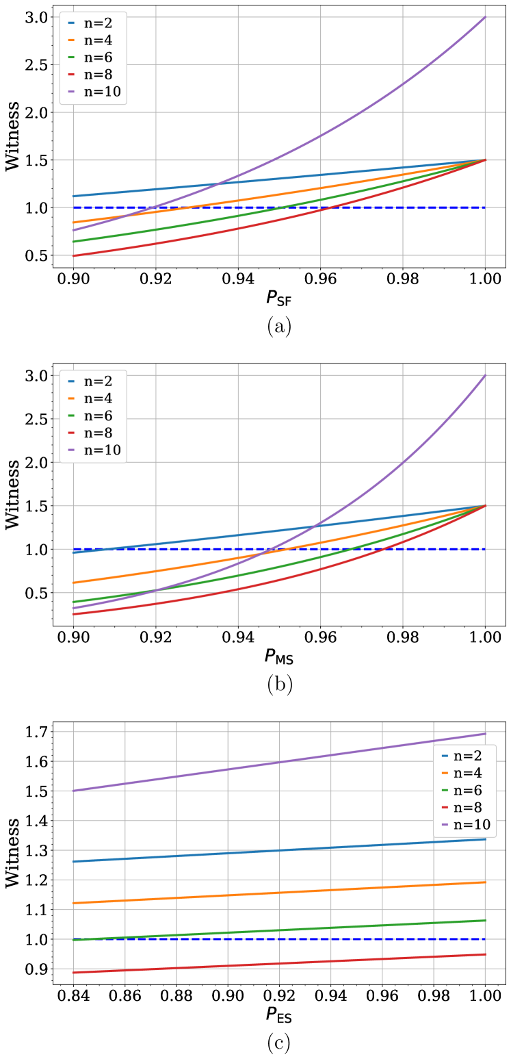
In the first step of Sec. III.2, starting from the all-zero state $\ket{00\cdots 0}$, one should flip the spins on the odd sites to prepare the Néel state in Eq. (4). There is the probability of a non-flip for the odd site, and also the probability of a wrong flip for the even site. For simplicity, we assume both error probabilities are equal, and denote the probability of the correct flip as $P_{\mathrm{SF}}$ for each site. In this case, the system is initially prepared into a mixture of different product states weighted with corresponding probabilities. In Fig. 5 (a), we plot the witness values of Eq. (16) for different subsystem size $n$ with respective to $P_{\mathrm{SF}}$. Similarly, in the final measurement, the probability to measure the spin of single atom correctly is denoted as $P_{\mathrm{MS}}$. That is, there is probability $1-P_{\mathrm{MS}}$ to recognize $\ket{0}$ as $\ket{1}$ or vice versa. The witness value with respective to $P_{\mathrm{MS}}$ is shown in Fig. 5 (b). From these two figures, we found that the witness values are the same for the subsystem with the same qubit number, for example, $n=2$ case with $\rho_{1,2}$ and $\rho_{1,3}$. When there is no error, say $P_{\mathrm{SF}}=1$ and $P_{\mathrm{MS}}=1$, all the witness values return $1.5$ for all the subsystems, except the whole system with the value $3$. One can see that even though there is some error, the witness can detect the entanglement as the value is larger than $1$. For larger subsystems, the values decay faster with $P_{\mathrm{SF}}$ and $P_{\mathrm{MS}}$.

Similar as the six-qubit case discussed in Sec. III.4, here for total system size $N=10$, one only needs to measure the witness for $\{\rho_{1,2},\rho_{1,3},\rho_{1,2,3,4},\rho_{1,2,3,5},\rho_{1,2,3,4,5,6},\\ \rho_{1,2,3,4,5,7},\rho_{7,8,9,10},\rho_{8,10},\rho_{9,10}\}$ to verify the full entanglement. As a result, the result of the subsystems with at most $n=6$ qubits decides the lower bound of the operation fidelity. According to Fig. 5 (a) and (b), the bounds are 0.95 and 0.97 for $P_{\mathrm{SF}}$ and $P_{\mathrm{MS}}$ respectively.

At last, in Fig. 5 (c), we study the influence of the fidelity of the entangling step between the above two steps by taking $P_{\mathrm{SF}}=0.98$ and $P_{\mathrm{MS}}=0.985$. Here we assume that this operation has a probability $P_{\mathrm{ES}}$ to be performed perfectly while it contributes zero to the witness with probability $1-P_{\mathrm{ES}}$, that is, essentially outputs a maximal mixed state. As shown in Fig. 5 (c), the full entanglement could be verified when the fidelity of entangling step exceeds $0.85$.

References

- Nielsen and Chuang [2011] Michael A. Nielsen and Isaac L. Chuang, Quantum Computation and Quantum Information: 10th Anniversary Edition, 10th ed. (Cambridge University Press, New York, NY, USA, 2011).
- Horodecki et al. [2009] Ryszard Horodecki, Paweł Horodecki, Michał Horodecki, and Karol Horodecki, “Quantum entanglement,” Rev. Mod. Phys. 81, 865–942 (2009).
- Monz et al. [2011] Thomas Monz et al., “14-qubit entanglement: Creation and coherence,” Phys. Rev. Lett. 106 (2011).
- Nigg et al. [2014] D. Nigg et al., “Quantum computations on a topologically encoded qubit,” Science 345, 302–305 (2014).
- Friis et al. [2018] Nicolai Friis et al., “Observation of entangled states of a fully controlled 20-qubit system,” Phys. Rev. X 8 (2018).
- Wang et al. [2018a] Xi-Lin Wang et al., “18-qubit entanglement with six photons’ three degrees of freedom,” Phys. Rev. Lett. 120 (2018a).
- Zhong et al. [2018] Han-Sen Zhong et al., “12-photon entanglement and scalable scattershot boson sampling with optimal entangled-photon pairs from parametric down-conversion,” Phys. Rev. Lett. 121 (2018).
- Omran et al. [2019] A. Omran et al., “Generation and manipulation of schrödinger cat states in rydberg atom arrays,” Science 365, 570–574 (2019).
- Gong et al. [2019] Ming Gong et al., “Genuine 12-qubit entanglement on a superconducting quantum processor,” Phys. Rev. Lett. 122 (2019).
- Wei et al. [2020] Ken X. Wei et al., “Verifying multipartite entangled greenberger-horne-zeilinger states via multiple quantum coherences,” Phys. Rev. A 101 (2020).
- Song et al. [2019] Chao Song et al., “Generation of multicomponent atomic schrödinger cat states of up to 20 qubits,” Science 365, 574–577 (2019).
- Zhang et al. [2017] J. Zhang et al., “Observation of a many-body dynamical phase transition with a 53-qubit quantum simulator,” Nature 551, 601–604 (2017).
- Arute et al. [2019] Frank Arute et al., “Quantum supremacy using a programmable superconducting processor,” Nature 574, 505–510 (2019).
- Preskill [2018] John Preskill, “Quantum Computing in the NISQ era and beyond,” Quantum 2, 79 (2018).
- Bloch et al. [2012] Immanuel Bloch, Jean Dalibard, and Sylvain Nascimbène, “Quantum simulations with ultracold quantum gases,” Nat. Phys. 8, 267–276 (2012).
- Jaksch et al. [1998] D. Jaksch, C. Bruder, J. I. Cirac, C. W. Gardiner, and P. Zoller, “Cold bosonic atoms in optical lattices,” Phys. Rev. Lett. 81, 3108–3111 (1998).
- Greiner et al. [2002] Markus Greiner, Olaf Mandel, Tilman Esslinger, Theodor W. Hänsch, and Immanuel Bloch, “Quantum phase transition from a superfluid to a mott insulator in a gas of ultracold atoms,” Nature 415, 39–44 (2002).
- Jaksch et al. [1999] D. Jaksch, H.-J. Briegel, J. I. Cirac, C. W. Gardiner, and P. Zoller, “Entanglement of atoms via cold controlled collisions,” Phys. Rev. Lett. 82, 1975–1978 (1999).
- Mandel et al. [2003] Olaf Mandel, Markus Greiner, Artur Widera, Tim Rom, Theodor W. Hänsch, and Immanuel Bloch, “Controlled collisions for multi-particle entanglement of optically trapped atoms,” Nature 425, 937–940 (2003).
- Raussendorf and Briegel [2001a] Robert Raussendorf and Hans J. Briegel, “A one-way quantum computer,” Phys. Rev. Lett. 86, 5188–5191 (2001a).
- Raussendorf et al. [2003] Robert Raussendorf, Daniel E. Browne, and Hans J. Briegel, “Measurement-based quantum computation on cluster states,” Phys. Rev. A 68, 022312 (2003).
- Trotzky et al. [2008] S. Trotzky et al., “Time-resolved observation and control of superexchange interactions with ultracold atoms in optical lattices,” Science 319, 295–299 (2008).
- Anderlini et al. [2007] Marco Anderlini, Patricia J. Lee, Benjamin L. Brown, Jennifer Sebby-Strabley, William D. Phillips, and J. V. Porto, “Controlled exchange interaction between pairs of neutral atoms in an optical lattice,” Nature 448, 452–456 (2007).
- Dai et al. [2016] Han-Ning Dai et al., “Generation and detection of atomic spin entanglement in optical lattices,” Nat. Phys. 12, 783–787 (2016).
- Scholl et al. [2021] Pascal Scholl et al., “Quantum simulation of 2D antiferromagnets with hundreds of Rydberg atoms,” Nature 595, 233–238 (2021).
- Scholl et al. [2022] P. Scholl et al., “Microwave engineering of programmable hamiltonians in arrays of rydberg atoms,” PRX Quantum 3, 020303 (2022).
- Weitenberg et al. [2011] Christof Weitenberg et al., “Single-spin addressing in an atomic mott insulator,” Nature 471, 319–324 (2011).
- Bakr et al. [2009] Waseem S. Bakr, Jonathon I. Gillen, Amy Peng, Simon Fölling, and Markus Greiner, “A quantum gas microscope for detecting single atoms in a hubbard-regime optical lattice,” Nature 462, 74–77 (2009).
- Sherson et al. [2010] Jacob F. Sherson, Christof Weitenberg, Manuel Endres, Marc Cheneau, Immanuel Bloch, and Stefan Kuhr, “Single-atom-resolved fluorescence imaging of an atomic mott insulator,” Nature 467, 68–72 (2010).
- Parsons et al. [2015] Maxwell F. Parsons, Florian Huber, Anton Mazurenko, Christie S. Chiu, Widagdo Setiawan, Katherine Wooley-Brown, Sebastian Blatt, and Markus Greiner, “Site-resolved imaging of FermionicLi6in an optical lattice,” Phys. Rev. Lett. 114 (2015).
- Cheuk et al. [2015] Lawrence W. Cheuk et al., “Quantum-gas microscope for fermionic atoms,” Phys. Rev. Lett. 114 (2015).
- Haller et al. [2015] Elmar Haller et al., “Single-atom imaging of fermions in a quantum-gas microscope,” Nat. Phys. 11, 738–742 (2015).
- Vogel and Risken [1989] K. Vogel and H. Risken, “Determination of quasiprobability distributions in terms of probability distributions for the rotated quadrature phase,” Phys. Rev. A 40, 2847–2849 (1989).
- Paris and Rehacek [2004] M. Paris and J. (eds) Rehacek, “Quantum state estimation,” Lect. Notes Phys. (2004).
- Terhal [2001] Barbara M. Terhal, “A family of indecomposable positive linear maps based on entangled quantum states,” Linear Algebra Appl. 323, 61 – 73 (2001).
- Guhne and Toth [2009] Otfried Guhne and Geza Toth, “Entanglement detection,” Phys. Rep. 474, 1 – 75 (2009).
- Friis et al. [2019] Nicolai Friis, Giuseppe Vitagliano, Mehul Malik, and Marcus Huber, “Entanglement certification from theory to experiment,” Nat. Rev. Phys. 1, 72–87 (2019).
- Tóth et al. [2009] Géza Tóth, Witlef Wieczorek, Roland Krischek, Nikolai Kiesel, Patrick Michelberger, and Harald Weinfurter, “Practical methods for witnessing genuine multi-qubit entanglement in the vicinity of symmetric states,” New J. Phys. 11, 083002 (2009).
- Tóth et al. [2010] G. Tóth, W. Wieczorek, D. Gross, R. Krischek, C. Schwemmer, and H. Weinfurter, “Permutationally invariant quantum tomography,” Phys. Rev. Lett. 105, 250403 (2010).
- Zhou et al. [2019a] You Zhou, Chenghao Guo, and Xiongfeng Ma, “Decomposition of a symmetric multipartite observable,” Phys. Rev. A 99, 052324 (2019a).
- Tóth and Gühne [2005a] Géza Tóth and Otfried Gühne, “Detecting genuine multipartite entanglement with two local measurements,” Phys. Rev. Lett. 94, 060501 (2005a).
- Knips et al. [2016] Lukas Knips, Christian Schwemmer, Nico Klein, Marcin Wieśniak, and Harald Weinfurter, “Multipartite entanglement detection with minimal effort,” Phys. Rev. Lett. 117, 210504 (2016).
- Zhou et al. [2019b] You Zhou, Qi Zhao, Xiao Yuan, and Xiongfeng Ma, “Detecting multipartite entanglement structure with minimal resources,” npj Quantum Inf. 5, 83 (2019b).
- Sebby-Strabley et al. [2006] J. Sebby-Strabley, M. Anderlini, P. S. Jessen, and J. V. Porto, “Lattice of double wells for manipulating pairs of cold atoms,” Phys. Rev. A 73 (2006).
- Lee et al. [2007] P. Lee, M. Anderlini, B. Brown, J. Sebby-Strabley, W. Phillips, and J. Porto, “Sublattice addressing and spin-dependent motion of atoms in a double-well lattice,” Phys. Rev. Lett. 99 (2007).
- Trotzky et al. [2010] Stefan Trotzky, Yu-Ao Chen, Ute Schnorrberger, Patrick Cheinet, and Immanuel Bloch, “Controlling and detecting spin correlations of ultracold atoms in optical lattices,” Phys. Rev. Lett. 105 (2010).
- Lohse et al. [2015] M. Lohse, C. Schweizer, O. Zilberberg, M. Aidelsburger, and I. Bloch, “A thouless quantum pump with ultracold bosonic atoms in an optical superlattice,” Nat. Phys. 12, 350–354 (2015).
- Duan et al. [2003] L.-M. Duan, E. Demler, and M. D. Lukin, “Controlling spin exchange interactions of ultracold atoms in optical lattices,” Phys. Rev. Lett. 91 (2003).
- Yang et al. [2020] Bing Yang et al., “Cooling and entangling ultracold atoms in optical lattices,” Science , eaaz6801 (2020).
- Yang et al. [2017] Bing Yang, Han-Ning Dai, Hui Sun, Andreas Reingruber, Zhen-Sheng Yuan, and Jian-Wei Pan, “Spin-dependent optical superlattice,” Phys. Rev. A 96 (2017).
- Vaucher et al. [2008] B Vaucher, A Nunnenkamp, and D Jaksch, “Creation of resilient entangled states and a resource for measurement-based quantum computation with optical superlattices,” New J. Phys. 10, 023005 (2008).
- Parsons et al. [2016] Maxwell F. Parsons, Anton Mazurenko, Christie S. Chiu, Geoffrey Ji, Daniel Greif, and Markus Greiner, “Site-resolved measurement of the spin-correlation function in the fermi-hubbard model,” Science 353, 1253–1256 (2016).
- Boll et al. [2016] Martin Boll et al., “Spin- and density-resolved microscopy of antiferromagnetic correlations in fermi-hubbard chains,” Science 353, 1257–1260 (2016).
- Wang et al. [2018b] Yuanhao Wang, Ying Li, Zhang-qi Yin, and Bei Zeng, “16-qubit ibm universal quantum computer can be fully entangled,” npj Quantum Inf. 4, 46 (2018b).
- Gühne and Tóth [2009] Otfried Gühne and Géza Tóth, “Entanglement detection,” Physics Reports 474, 1–75 (2009).
- Chen and Lo [2007] Kai Chen and Hoi-Kwong Lo, “Multi-partite quantum cryptographic protocols with noisy GHZ states,” Quantum Inf. Comput. 7, 689–715 (2007).
- Brunner et al. [2014] Nicolas Brunner, Daniel Cavalcanti, Stefano Pironio, Valerio Scarani, and Stephanie Wehner, “Bell nonlocality,” Reviews of Modern Physics 86, 419 (2014).
- Wehner et al. [2018] Stephanie Wehner, David Elkouss, and Ronald Hanson, “Quantum internet: A vision for the road ahead,” Science 362, eaam9288 (2018).
- Perseguers et al. [2013] S Perseguers, G J Lapeyre, D Cavalcanti, M Lewenstein, and A Acín, “Distribution of entanglement in large-scale quantum networks,” Rep. Prog. Phys. 76, 096001 (2013).
- Giovannetti et al. [2011] Vittorio Giovannetti, Seth Lloyd, and Lorenzo Maccone, “Advances in quantum metrology,” Nat. Photonics 5, 222–229 (2011).
- Raussendorf and Briegel [2001b] Robert Raussendorf and Hans J. Briegel, “A one-way quantum computer,” Phys. Rev. Lett. 86, 5188–5191 (2001b).
- Gühne et al. [2007] Otfried Gühne, Chao-Yang Lu, Wei-Bo Gao, and Jian-Wei Pan, “Toolbox for entanglement detection and fidelity estimation,” Phys. Rev. A 76, 030305(R) (2007).
- Zhao et al. [2019] Qi Zhao, Gerui Wang, Xiao Yuan, and Xiongfeng Ma, “Efficient and robust detection of multipartite greenberger-horne-zeilinger-like states,” Phys. Rev. A 99, 052349 (2019).
- Zhang et al. [2021] Yihong Zhang, Yifan Tang, You Zhou, and Xiongfeng Ma, “Efficient entanglement generation and detection of generalized stabilizer states,” Phys. Rev. A 103, 052426 (2021).
- Tóth and Gühne [2005b] Géza Tóth and Otfried Gühne, “Entanglement detection in the stabilizer formalism,” Phys. Rev. A 72, 022340 (2005b).
- Asadian et al. [2016] Ali Asadian, Paul Erker, Marcus Huber, and Claude Klöckl, “Heisenberg-weyl observables: Bloch vectors in phase space,” Phys. Rev. A 94, 010301 (2016).
- Bourennane et al. [2004] Mohamed Bourennane et al., “Experimental detection of multipartite entanglement using witness operators,” Phys. Rev. Lett. 92, 087902 (2004).