\savesymbol

iint \savesymbolopenbox \restoresymbolTXFiint \restoresymbolTXFopenbox

A Scaling Approach to Elliptic Theory for Geometrically-Natural Differential Operators with Sobolev-Type Coefficients

Michael Holst, David Maxwell and Gantumur Tsogtgerel

(June 28, 2023)

Abstract

We develop local elliptic regularity for operators having coefficients in a range of Sobolev-type function spaces (Bessel potential, Sobolev-Slobodeckij, Triebel-Lizorkin, Besov) where the coefficients have a regularity structure typical of operators in geometric analysis. The proofs rely on a nonstandard technique using rescaling estimates and apply to operators having coefficients with low regularity. For each class of function space for an operator’s coefficients, we exhibit a natural associated range of function spaces of the same type for the domain of the operator and we provide regularity inference along with interior estimates. Additionally, we present a unified set of multiplication results for the function spaces we consider.

^†^†2020 Mathematics Subject Classification. Primary: 35B65. Secondary: 35J47, 35J48, 46F10.^†^†Keywords: elliptic regularity, Bessel potential, Sobolev-Slobodeckij, Triebel-Lizorkin, Besov, multiplication

1 Introduction

Elliptic differential operators associated with Riemannian metrics having limited regularity arise naturally in the construction of initial data in general relativity. Moreover, because of connections with the associated evolution problem, it is natural to work with metrics having regularity measured in Sobolev-type scales, and with a non-integral number of derivatives [KR05][ST05][Ma06]. In this paper we develop a largely self-contained account of the mapping properties and local elliptic regularity theory for differential operators having coefficients in any one of a broad category of Sobolev-type spaces, including spaces with non-integral levels of differentiability, where the coefficients also admit a regularity structure typical of geometric differential operators. For each category of function spaces considered, we allow for coefficients with low regularity, and our approach to local elliptic theory is apparently novel in this context, relying on rescaling estimates for Sobolev-type spaces to reduce the problem to that of constant-coefficient operators.

Local elliptic regularity is a well-established subject, with a wealth of results available in a number of contexts, even in low-regularity settings. For second-order scalar elliptic operators in divergence form [Tr73] treats a form of elliptic regularity assuming only that the coefficients are measurable, although only for a very limited set of (operator-dependent) function spaces. A related theory appears in the text [GT01] that applies to a range of integer-based Sobolev spaces under progressively stronger hypotheses on the coefficients of the elliptic operator. See also [Gi93], which contains analogous results that apply to systems of equations. Spaces with a non-integral number of derivatives include the $L^{2}$ -based spaces $H^{s}$ which appear naturally in hyperbolic problems as well as their generalizations: Bessel potential spaces $H^{s,p}$ , Sobolev-Slobodeckij spaces $W^{s,p}$ , Triebel-Lizorkin spaces $F^{s,p}_{q}$ , and Besov spaces $B^{s,p}_{q}$ . So long as the differential operators involved have smooth coefficients, elliptic theory for these spaces can be found in [Tr10]. For less regular coefficients, one is led to the theory of pseudodifferential operators with non-smooth symbols and paradifferential calculus. See, e.g., [Ta91] and [Ma88]. Nevertheless, this theory is somewhat technical, and it can be difficult for non-practitioners to apply it immediately to the specific class of questions addressed in the current work.

Within the mathematical relativity literature one finds instead a sequence of custom-made regularity theorems for second-order operators associated with with a metric $g$ on a domain of dimension $n\geq 3$ :

•

[CC81]: $g\in W^{k,2}$ with $k\in\mathbb{N}$ , $k>n/2+1$ and hence possessing Hölder continuous derivatives,
•

[Ch04][Ma05]: $g\in W^{k,p}$ with $k\in\mathbb{N}$ , $k\geq 2$ and $k>n/p$ and hence Hölder continuous,
•

[Ma06]: $g\in H^{s}$ with $s\in\mathbb{R}$ , $s>n/2$ and hence Hölder continuous,
•

[HNT09] $g\in W^{s,p}$ with $s\in\mathbb{R}$ , $s\geq 1$ and $s>n/p$ and hence Hölder continuous.

Although [Ma06] was the first work in this context to treat spaces with a fractional number of derivatives, its limited focus on the $L^{2}$ setting meant that it did not recover the full set of earlier results. By contrast, [HNT09] recovers prior results fully, but its main regularity result, Lemma 32, contains an error that is not straightforward to correct. Moreover, although Sobolev-Slobodeckij spaces $W^{s,p}$ are a reasonable choice for interpolating between integer-based Sobolev spaces, Bessel potential spaces $H^{s,p}$ enjoy better interpolation and embedding properties and are a compelling alternative. Hence it would be desirable to extend the results above to other classes of function spaces, and indeed our work here concerning Bessel potential spaces provides the elliptic theory used by the recent preprint [ALM22], which treats geometric operators on asymptotically hyperbolic manifolds.

Our main results concern local elliptic regularity for differential operators having coefficients in any of the Sobolev-type spaces $H^{s,p}$ , $W^{s,p}$ , $F^{s,p}_{q}$ and $B^{s,p}_{q}$ mentioned above. Although we use basic techniques from the theory of paraproducts in the proofs of some of our work, we do so with a minimum of theoretical overhead, and Section 3.2 contains a short survey of the few tools needed. Moreover, although Bessel potential spaces are a special case of Triebel-Lizorkin spaces and could have been dealt with as a consequence of the general theory, in Section 2 we present a simplified approach in the Bessel potential context that is free from paraproduct methods. This approach comes at the expense of establishing a less-than-sharp intermediate result on rescaling (Proposition 2.17 vs. Proposition 3.10), but this has no impact on the final regularity theory. Readers who are only interested in the Bessel potential case can stop reading at the end of Section 2 without needing to move on to the relative complexities of the more general function spaces.

In addition to extending the scope of [Ma06] and [HNT09] to a broader class of function spaces, the results of this paper strengthen our earlier work. Rather than simply obtaining a-priori estimates for functions with a known level of regularity, we obtain full regularity inference in the spirit of, e.g., [GT01] Theorem 8.8. Additionally, we have extended the range of parameters of the function spaces treated. This extension is only marginal in the generic case, but substantially extends the range of parameters whenever the operators involved omit low-order terms; see the discussion following Definition 2.4. Although we restrict our attention to interior regularity, the tools developed here are also sufficient to address boundary value problems. We have omitted these considerations, in part for simplicity of exposition: boundary traces generally lie in Besov spaces, which are among the most technical of the spaces we consider, and which we treat last. We will address boundary regularity in followup work.

Principal applications of elliptic regularity only apply to the range of Lebesgue exponents $1<p<\infty$ . Motivated by this, and again for the sake of simple exposition, we have avoided the edge cases of $F^{s,p}_{q}$ and $B^{s,p}_{q}$ where $p,q=1,\infty$ , much less the quasi-normed spaces where $p,q<1$ . We observe, however, that the multiplication rules of Theorems 3.5 and 5.4 and the rescaling estimates of Propositions 3.10 and 5.11 are candidates that could benefit from extending beyond the parameter ranges treated here.

1.1 Coefficient regularity structure

Differential operators in geometric analysis admit a representation in local coordinates in terms of coefficients that are universal expressions involving the values and derivatives of the coordinate representation $g_{ab}$ of a metric $g$ . The prototypical example is the Laplacian $\Delta_{g}$ associated with $g$ , which can be written in terms of the inverse metric $g^{ab}$ and the determinant $\sqrt{g}$ as

\Delta_{g}=g^{ab}\partial_{a}\partial_{b}+\sum_{a}\sqrt{g}\left(\partial_{a}\left(\frac{1}{\sqrt{g}}g^{ab}\right)\right)\partial_{b}.

The leading order coefficients have the regularity of $g_{ab}$ , whereas the next order coefficients involve first derivatives of $g_{ab}$ . More generally, consider the conformal Laplacian $\mathcal{C}_{g}$ of $g$ ,

\mathcal{C}_{g}=-c_{n}\Delta_{g}+R_{g}

where $c_{n}=-4(n-1)/(n-2)$ and where $R_{g}$ is the scalar curvature of the metric. If the coefficients of the metric lie in $W^{1,p}_{\rm loc}$ with $p>n$ , a computation using Hölder’s inequality and Sobolev embedding shows that $\mathcal{C}_{g}$ has the form

\mathcal{C}_{g}=-c_{n}g^{ab}\partial_{a}\partial_{b}+\beta^{a}\partial_{a}+\gamma

where

\displaystyle g^{ab}\in W^{1,p}_{\rm loc},\qquad\beta^{a}\in W^{0,p}_{\rm loc},\qquad\gamma\in W^{-1,p}_{\rm loc}.

In particular, the leading order coefficients have the regularity of the metric, and there is a loss of one derivative as we descend from one order of coefficient to the next. This leads us to consider elliptic $d^{\rm th}$ -order operators of the form

L=\sum_{|\alpha|\leq d}a^{\alpha}\partial_{\alpha}

(1.1)

where the top-most coefficients lie in a space $J^{s}$ with $s$ derivatives and more generally where each $a^{\alpha}\in J^{s-d+|\alpha|}$ . While this category of operator is not the most general possible in geometric analysis [St75], it is sufficiently broad to include many operators of interest, including Hodge Laplacians, the Lichnerowicz Laplacian [Be87], the vector Laplacian [Is95] and the conformal Laplacian, so long as $s\geq 1$ and so long as the underlying metric lies in a space sufficiently regular so as to ensure Hölder continuity. It also includes the class of geometric operators satisfying the hypotheses of Assumption P of [ALM22].

Given an operator of the form (1.1) with leading order coefficients in some space $J^{s}$ with $s$ derivatives, one wants to find compatible spaces $K^{\sigma}$ with $\sigma$ derivatives such that that $L:K^{\sigma}\to K^{\sigma-d}$ and such that local elliptic regularity holds: roughly that if $u$ is regular enough that $L$ can act on it, and if $Lu\in K^{\sigma-d}$ , then locally $u\in K^{\sigma}$ along with associated estimates. We establish this theory for elliptic operators of the form (1.1) where the topmost coefficients come from a space $J^{s}$ of one of the following types:

•

a Bessel potential space $H^{s,p}$ , in which case $K^{\sigma}$ is another Bessel potential space $H^{\sigma,q}$ (Section 2),
•

a Triebel-Lizorkin space $F^{s,p}_{q}$ , in which case $K^{\sigma}$ is another Triebel-Lizorkin space $F^{\sigma,a}_{b}$ (Section 3),
•

a Sobolev-Slobodeckij space $W^{s,p}$ , in which case $K^{\sigma}$ is another Sobolev-Slobodeckij space $W^{\sigma,q}$ (Section 4),
•

a Besov space $B^{s,p}_{q}$ , in which case $K^{\sigma}$ is another Besov space $B^{\sigma,a}_{b}$ (Section 5).

In all these cases, the space $J^{s}$ is restricted to be suitably regular so that its elements are Hölder continuous, and we give a careful description of the parameters determining the allowable spaces $K^{\sigma}$ .

1.2 Rescaling estimates

Our general approach is the same for all the function spaces considered, and in the specific case of Bessel potential spaces $H^{s,p}$ the core ingredients are:

1.

Multiplication properties for $H^{s,p}$ spaces, Theorem 2.5.
2.

Mapping properties: given an operator $L$ of the form (1.1) with leading coefficients in $H^{s,p}$ , for which spaces $H^{\sigma,q}$ does $L$ map $H^{\sigma,q}\to H^{\sigma-d,q}$ ? This is the content of Proposition 2.6.
3.

A rescaling estimate, described below.
4.

A coefficient freezing/blowup argument which uses the rescaling estimate to establish “regularity at a point”, Proposition 2.20.
5.

A partition of unity decomposition and bootstrap to obtain the main regularity result, Theorem 2.21.

Coefficient freezing as used in step 4 above is classical, but we use a nonstandard rescaling technique to manage the perturbations from the constant coefficient operator. To motivate this technique, consider the simplest case of integer-based Sobolev spaces on the unit ball $B_{1}\subset\mathbb{R}^{n}$ , and let $u\in W^{k,p}(B_{1})$ , where $k\in\mathbb{N}$ , $1<p<\infty$ . For $0<r\leq 1$ we define $u_{\{r\}}(x)=u(rx)$ , so $u_{\{r\}}$ rescales $u$ up from the ball of radius $r$ to the unit ball. Derivatives are damped under this rescaling operation, but the singularities permitted by $L^{p}$ spaces are enhanced, and a computation using Sobolev embedding and Hölder’s inequality shows

||u_{\{r\}}||_{W^{k,p}(B_{1})}\lesssim r^{\alpha}||u||_{W^{k,p}(B_{1})}

(1.2)

where $\alpha=\min(k-\frac{n}{p},0)$ , except in the marginal case $k=n/p$ , in which case we can take $\alpha$ to be any negative number. The cap $\alpha\leq 0$ appears in this estimate because of the constants, which are invariant under rescaling. However, if $k>n/p$ so that elements of $W^{k,p}(B_{1})$ are Hölder continuous, and if $f(0)=0$ , one can do better. Now estimate (1.2) holds with $\alpha=\min(k-n/p,1)$ , except in the marginal case $k=n/p+1$ , in which case we can use any $\alpha<1$ . Regardless, if $k>n/p$ and if $f(0)=0$ , estimate (1.2) holds for some $\alpha>0$ .

Now consider a differential operator $L=\sum_{|\beta|\leq d}a^{\beta}\partial_{\beta}$ with coefficients $a^{\beta}\in W^{k-d+|\beta|,p}(B_{1})$ and with $k>n/p$ . The leading order coefficients lie in $W^{k,p}(B_{1})$ and are therefore Hölder continuous. Hence we can define the principal part of $L$ at $0$ ,

L_{0}=\sum_{|\beta|=d}a^{\beta}(0)\partial_{\beta}.

If $u$ is a distribution that is regular enough that $L$ can act on it, a computation shows that

\displaystyle r^{d}(Lu)_{{\{r\}}}

\displaystyle=L_{0}u_{\{r\}}+\underbrace{\sum_{|\beta|=d}(a^{\beta}-a^{\beta}(0))_{\{r\}}\partial_{\beta}u_{\{r\}}}_{:=B_{[r]}u_{\{r\}}}+\underbrace{\sum_{|\beta|<d}r^{d-|\beta|}a^{\beta}_{{\{r\}}}\partial_{\beta}u_{\{r\}}}_{:=C_{[r]}u_{\{r\}}}.

The aim at this point is to show that by taking $r$ sufficiently small, the coefficients of the perturbations $B_{[r]}$ and $C_{[r]}$ can be made as small as desired so that a parametrix for $L_{0}$ can be employed to deduce regularity properties of $u_{\{r\}}$ , and this is where the rescaling estimate (1.2) is needed. Using the structural hypothesis $a_{\beta}\in W^{k-d+|\beta|,p}(B_{1})$ along with the rescaling estimate (1.2) we find, except in marginal cases where an unimportant adjustment is needed, that the coefficients of $C_{[r]}$ satisfy

||r^{d-|\beta|}(a_{\beta})_{\{r\}}||_{W^{k-d+|\beta|,p}(B_{1})}\lesssim r^{d-|\beta|}r^{\min(k-d+|\beta|-n/p,0)}||a_{\beta}||_{W^{k-d+|\beta|,p}(B_{1})}.

Since $|\beta|<d$ for each of these coefficients, and since $k>n/p$ , we obtain

r^{d-|\beta|}r^{\min(k-d+\beta-n/p,0)}=r^{\min(k-n/p,d-|\beta|)}=r^{\epsilon}

for some $\epsilon>0$ . Hence the coefficients of $C_{[r]}$ scale away as $r\to 0$ . On the other hand, the high order perturbation coefficients $a^{\beta}-a^{\beta}(0)$ lie in $W^{k,p}(B_{1})$ with $k>n/p$ and vanish at $0$ , so the improved variation of the scaling estimate (1.2) again shows that the coefficients of $B_{[r]}$ vanish as $r\to 0$ .

Propositions 3.10 and 5.11 show that estimate (1.2) generalizes to Triebel-Lizorkin and Besov spaces respectively. For Triebel-Lizorkin spaces, the proof requires elementary techniques from Littlewood-Paley theory and paramultiplication, and the necessary background is recalled in Section 3.2 prior to the proof of Proposition 3.10. The analogous results for Besov spaces follow from the Triebel-Lizorkin result and interpolation. As mentioned above, in the interest of approachability, for Bessel potential spaces we use an alternative approach with a rescaling estimate, Proposition 2.17, that is not sharp, but which admits an elementary proof that is independent of Littlewood-Paley theory.

1.3 Multiplication

Mapping properties of differential operators with coefficients in Sobolev-type spaces depend on pointwise multiplication rules that determine when a product of factors from two given function spaces lies in a third space. There is an extensive literature on this subject, including [Pa68] [Zo77] [Am91] [ST95] [RS96] [Jo95] [BH21] that contains individual pieces of the theory we require. Chapter 4 of [RS96] is especially comprehensive. Where these works overlap, there is generally agreement on the hypotheses, but certain edge cases are treated, or not, by different authors. Rather than attempt to assemble these disparate pieces into a coherent whole, we include a self-contained proof of multiplication rules for Triebel-Lizorkin spaces, Theorem 3.5, and for Besov spaces, Theorem 5.4, in the appendices. Corresponding rules for Bessel potential spaces and Sobolev-Slobodeckij spaces, Theorems 2.5 and 4.2 respectively, follow as corollaries. The proofs rely on the same elementary Littlewood-Paley/paramultiplication techniques that we use to obtain the rescaling estimates of Section 3.2. Although we have limited our analysis to the region $1<p,q<\infty$ for the spaces $F^{s,p}_{q}$ and $B^{s,p}_{q}$ , in this restricted setting we obtain a consistent set of hypotheses over all ranges of $s$ that are simpler in character, and that are at least as sharp, as what appears currently in the literature.

2 Coefficients in Bessel Potential Spaces

In this section we prove interior elliptic estimates for operators having coefficients in Bessel potential spaces, with a goal of presenting the result using a minimum of technology. The primary background requirements are:

•

standard facts about Sobolev spaces with integer orders of differentiability,
•

embedding, interpolation and duality theory for Bessel potential spaces,
•

multiplication rules for Bessel potential spaces, which we recall below, and
•

elementary tools from harmonic analysis needed to construct parametrices for elliptic operators with constant coefficients.

In particular, the approach is otherwise independent of Littlewood-Paley theory or the general theory of pseudodifferential operators, beyond what is required to define the spaces themselves.

Let $\mathcal{F}$ denote the Fourier transform and for $s\in\mathbb{R}$ let $D^{s}$ be the pseudodifferential operator given by

\mathcal{F}[D^{s}u](\xi)=(1+|\xi|^{2})^{s/2}\mathcal{F}[u](\xi).

Given $1<p<\infty$ and $s\in\mathbb{R}$ a tempered distribution $u$ on $\mathbb{R}^{n}$ belongs to the Bessel potential space $H^{s,p}(\mathbb{R}^{n})$ if $D^{-s}u\in L^{p}(\mathbb{R}^{n})$ , in which case

||u||_{H^{s,p}(\mathbb{R}^{n})}=||D^{-s}u||_{L^{p}(\mathbb{R}^{n})}.

We use the same notation for for distributions taking on values in a real vector space (e.g., $\mathbb{R}^{k}$ or $\mathbb{R}^{k\times k}$ ). When $k\in\mathbb{Z}$ , then $H^{k,p}(\mathbb{R}^{n})$ with this definition coincides with standard Sobolev spaces of distributions having derivatives laying in Lebesgue spaces.

Given an open set $\Omega\subseteq\mathbb{R}^{n}$ the space $H^{s,p}(\Omega)$ consists of restrictions of distributions in $H^{s,p}(\mathbb{R}^{n})$ to $\Omega$ and is given the quotient norm. That is,

||u||_{H^{s,p}(\Omega)}=\inf\{||\hat{u}||_{H^{s,p}(\mathbb{R}^{n})}:\hat{u}\in H^{s,p}(\mathbb{R}^{n}),\hat{u}|_{\Omega}=u\}.

We say an open set $\Omega$ is a $C^{\infty}$ domain if each point in the boundary admits an open ball centered at it and a diffeomorphism from it to an open subset of $\mathbb{R}^{n}$ such that the image of the intersection of $\Omega$ with the ball is a simply connected subset of the upper half space $\mathbb{R}^{n,+}$ . If $\Omega$ is a bounded $C^{\infty}$ domain and if $k\in\mathbb{Z}$ , then $H^{k,p}(\Omega)$ coincides with the usual integer-based Sobolev spaces.

We have the following embedding, interpolation, and duality properties of Bessel potential spaces, which are special cases of the same results cited in Section 3 for the more general Triebel-Lizorkin spaces.

Proposition 2.1.

Assume $1<p,p_{1},p_{2}<\infty$ and $s,s_{1},s_{2}\in\mathbb{R}$ , and suppose $\Omega$ is a bounded open set in $\mathbb{R}^{n}$ .

1.

If $s_{1}>s_{2}$ then $H^{s_{1},p}(\mathbb{R}^{n})\hookrightarrow H^{s_{2},p}(\mathbb{R}^{n})$ and $H^{s_{1},p}(\Omega)\hookrightarrow H^{s_{2},p}(\Omega)$ .
2.

If $p_{1}\geq p_{2}$ then $H^{s,p_{1}}(\Omega)\hookrightarrow H^{s,p_{2}}(\Omega)$ .
3.

If $s_{1}>s_{2}$ and $\frac{1}{p_{1}}-\frac{s_{1}}{n}=\frac{1}{p_{2}}-\frac{s_{2}}{n}$ then $H^{s_{1},p_{1}}(\mathbb{R}^{n})\hookrightarrow H^{s_{2},p_{2}}(\mathbb{R}^{n})$ .
4.

If $s_{1}>s_{2}$ and $\frac{1}{p_{1}}-\frac{s_{1}}{n}\leq\frac{1}{p_{2}}-\frac{s_{2}}{n}$ then $H^{s_{1},p_{1}}(\Omega)\hookrightarrow H^{s_{2},p_{2}}(\Omega)$ .
5.

If $0<\alpha<1$ then $H^{\frac{n}{p}+\alpha,p}(\mathbb{R}^{n})\hookrightarrow C^{0,\alpha}(\mathbb{R}^{n})$ and $H^{\frac{n}{p}+\alpha,p}(\Omega)\hookrightarrow C^{0,\alpha}(\Omega)$ .

In the final embedding above, $C^{0,\alpha}(\mathbb{R}^{n})$ denotes the Hölder space with norm $||u||_{C^{0,\alpha}(\mathbb{R}^{n})}=||u||_{L^{\infty}(\mathbb{R}^{n})}+\sup_{x\neq y}\left|\frac{f(x)-f(y)}{|x-y|^{\alpha}}\right|$ , with an analogous norm for functions defined on $\Omega$ .

Proposition 2.2.

Assume $1<p_{1},p_{2}<\infty$ and $s_{1},s_{2}\in\mathbb{R}$ , and suppose $\Omega$ is either $\mathbb{R}^{n}$ or is a bounded $C^{\infty}$ domain in $\mathbb{R}^{n}$ . For $0<\theta<1$ ,

[H^{s_{1},p_{1}}(\Omega),H^{s_{2},p_{2}}(\Omega)]_{\theta}=H^{s,p}(\Omega)

where

s=(1-\theta)s_{1}+\theta s_{2},\quad\frac{1}{p}=(1-\theta)\frac{1}{p_{1}}+\theta\frac{1}{p_{2}}

Proposition 2.3.

Assume $1<p<\infty$ and $s\in\mathbb{R}$ . The bilinear map $C^{\infty}(\mathbb{R}^{n})\times C^{\infty}(\mathbb{R}^{n})\to\mathbb{R}$ given by $\left<f,g\right>:=\int_{\Omega}fg$ extends to a continuous bilinear map $F^{s,p}_{q}(\mathbb{R}^{n})\times F^{-s,p^{*}}_{q^{*}}(\mathbb{R}^{n})\to\mathbb{R}$ where $1/p^{*}=1-1/p$ and $1/q^{*}=1-1/q$ . Moreover, $f\mapsto\left<f,\cdot\right>$ is a continuous identification of $F^{s,p}_{q}(\mathbb{R}^{n})$ with $(F^{-s,p^{*}}_{q^{*}}(\mathbb{R}^{n}))^{*}$ .

2.1 Mapping properties

The following definition encodes the regularity structure of the coefficients of differential operators appearing frequently in geometric analysis.

Definition 2.4.

Consider a $d^{\rm th}$ order differential operator on an open set $\Omega\subseteq\mathbb{R}^{n}$ ,

L=\sum_{|\alpha|\leq d}a^{\alpha}\partial_{\alpha}

where the coefficients are $\mathbb{R}^{k\times k}$ -valued for a system of $k$ variables. We say that $L$ is of class $\mathcal{L}^{d}(H^{s,p};\Omega)$ for some $s\in\mathbb{R}$ and $1<p<\infty$ if each

a^{\alpha}\in H^{s+|\alpha|-d,p}(\Omega).

If $L$ omits terms of order lower than $d_{0}$ for some $0\leq d_{0}\leq d$ , i.e.,

L=\sum_{d_{0}\leq|\alpha|\leq d}a^{\alpha}\partial_{\alpha},

we say $L\in\mathcal{L}_{d_{0}}^{d}(H^{s,p};\Omega)$ .

To motivate the roles of the pair of indices $d$ and $d_{0}$ in the previous definition, recall from the introduction the conformal Laplacian $\mathcal{C}_{g}=-c_{n}\Delta_{g}+R[g]$ of a metric $g$ on a bounded $C^{\infty}$ domain $\Omega$ . An elementary computation using Sobolev embedding shows that if $g\in H^{1,p}(\Omega)$ with $p>n$ then $\mathcal{C}_{g}$ is of class $\mathcal{L}^{2}(H^{1,p};\Omega)$ . The low-order term is the scalar curvature $R[g]\in H^{-1,p}(\Omega)$ and its presence restricts the set of spaces that $\mathcal{C}_{g}$ can act on: functions in these spaces must possess at least one derivative. By contrast, the ordinary Laplacian for the same metric has no zero-order term and consequently is an operator of class $\mathcal{L}^{2}_{1}(H^{1,p};\Omega)$ . Moreover, one can show that it acts on a broader class of spaces and, for example, defines a map $L^{p}(\Omega)\to H^{-2,p}(\Omega)$ . Hence, in addition to the order $d$ of the differential operator we also track the order $d_{0}$ of the term with the lowest number of derivatives appearing in the operator.

Consider an operator $L$ of class $\mathcal{L}_{d_{0}}^{d}(H^{s,p};\Omega)$ . It defines a map from $C^{\infty}(\overline{\Omega})$ , the set of smooth functions on $\Omega$ admitting smooth extensions to $\mathbb{R}^{n}$ , to the set $D^{\prime}(\Omega)$ of distributions on $\Omega$ , and we wish to establish finer-grained mapping properties. Specifically, we would like to determine the indices $(\sigma,q)\in\mathbb{R}\times(1,\infty)$ such that $L$ is continuous $H^{\sigma,q}(\Omega)\to H^{\sigma-d,q}(\Omega)$ .

The following result on multiplication of Bessel potential spaces is the tool needed to establish these mapping properties. It can be readily proved for integral orders of differentiability using only Sobolev embedding and duality arguments, and a slightly less sharp version that would, in fact, be sufficient for our purposes can be proved with interpolation techniques ([BH21] Theorem 5.1). See also [Pa68], the original reference for multiplication of Bessel potential spaces, which also considers the case of more than two factors. The statement below is a special case of the multiplication rules for the broader class of Triebel-Lizorkin spaces proved in Appendix A.

Theorem 2.5.

Let $\Omega$ be a bounded open subset of $\mathbb{R}^{n}$ . Suppose $1<p_{1},p_{2},q<\infty$ and $s_{1},s_{2},\sigma\in\mathbb{R}$ . Let $r_{1},r_{2}$ and $r$ be defined by

\frac{1}{r_{1}}=\frac{1}{p_{1}}-\frac{s_{1}}{n},\qquad\frac{1}{r_{2}}=\frac{1}{p_{2}}-\frac{s_{2}}{n},\quad\text{\rm and}\quad\frac{1}{r}=\frac{1}{q}-\frac{\sigma}{n}.

Pointwise multiplication of $C^{\infty}(\overline{\Omega})$ functions extends to a continuous bilinear map $H^{s_{1},p_{1}}(\Omega)\times H^{s_{2},p_{2}}(\Omega)\rightarrow H^{\sigma,q}(\Omega)$ so long as

$\displaystyle s_{1}+s_{2}$	$\displaystyle\geq 0$	(2.1)
$\displaystyle\min({s_{1},s_{2}})$	$\displaystyle\geq\sigma$	(2.2)
$\displaystyle\max\left(\frac{1}{r_{1}},\frac{1}{r_{2}}\right)$	$\displaystyle\leq\frac{1}{r}$	(2.3)
$\displaystyle\frac{1}{r_{1}}+\frac{1}{r_{2}}$	$\displaystyle\leq 1$	(2.4)
$\displaystyle\frac{1}{r_{1}}+\frac{1}{r_{2}}$	$\displaystyle\leq\frac{1}{r}$	(2.5)

with inequality (2.5) strict if $\min(1/r_{1},1/r_{2},1-1/r)=0$ .

There are admittedly a large number of conditions in the previous result, but they all have an easy interpretation. For a pair $(\sigma,q)\in\mathbb{R}\times(1,\infty)$ we call

\frac{1}{r}=\frac{1}{q}-\frac{\sigma}{n}

the Lebesgue regularity of the pair, the terminology motivated by the observation that if $0<1/r<1$ then Sobolev embedding implies $H^{\sigma,q}_{\rm loc}(\mathbb{R}^{n})$ embeds in $L^{r}_{\rm loc}(\mathbb{R}^{n})$ . Using this vocabulary, the conditions (2.1)–(2.5) are, loosely:

(2.1)

If one factor has a negative number of derivatives, the remaining factor must have at as many positive derivatives.
(2.2)

The product will not have, in general, more derivatives than either factor.
(2.3)

The product will not have, in general, better Lebesgue regularity than either factor.
(2.4)

$L^{1}$ is a least-regular barrier for multiplication of $L^{p}$ spaces. Note that in light of inequality (2.5) this condition only plays a role if $s<0$ .
(2.5)

The Lebesgue regularity of the product is consistent with multiplication of $L^{p}$ spaces. Strictness of this inequality is needed in edge cases because $L^{\infty}$ is not the right target space for borderline Sobolev embeddings.

Repeated applications of Theorem 2.5 imply the following mapping result, where we emphasize the new hypothesis $s>n/p$ which ensures, among other consequences, that the highest order coefficients of the differential operator are continuous.

Proposition 2.6.

Let $\Omega$ be a bounded open subset of $\mathbb{R}^{n}$ . Suppose $1<p,q<\infty$ , $s>n/p$ , $\sigma\in\mathbb{R}$ and $d,d_{0}\in\mathbb{Z}_{\geq 0}$ with $d\geq d_{0}$ . An operator of class $\mathcal{L}_{d_{0}}^{d}(H^{s,p};\Omega)$ extends from a map $C^{\infty}(\overline{\Omega})\mapsto\mathcal{D}^{\prime}(\Omega)$ to a continuous linear map $H^{\sigma,q}(\Omega)\mapsto H^{\sigma-d,q}(\Omega)$ so long as

	$\displaystyle\sigma$	$\displaystyle\in[d-s,s+d_{0}]$		(2.6)
	$\displaystyle\frac{1}{q}-\frac{\sigma}{n}$	$\displaystyle\in\left[\frac{1}{p}-\frac{s+d_{0}}{n},\frac{1}{p^{*}}-\frac{d-s}{n}\right]$		(2.6)

where $1/p^{*}=1-1/p$ is the conjugate Lebesgue exponent of $p$ . Moreover, the map $A$ between these spaces depends continuously on its coefficients $a^{\alpha}\in H^{s-d+\alpha,p}(\Omega)$ .

Conditions (2.6) on $\sigma$ and $q$ describe the natural Sobolev indices of spaces for an operator of class $\mathcal{L}_{d_{0}}^{d}(H^{s,p};\Omega)$ to act on, and it is convenient to have notation for this set.

Definition 2.7.

Suppose $1<p<\infty$ , $s\in\mathbb{R}$ and $d,d_{0}\in\mathbb{Z}_{\geq 0}$ with $d\geq d_{0}$ . The compatible Sobolev indices for an operator of class $\mathcal{L}_{d_{0}}^{d}(H^{s,p};\Omega)$ acting on a bounded open set $\Omega$ is the set

\mathcal{S}_{d_{0}}^{d}(H^{s,p})\subseteq\mathbb{R}\times(1,\infty)

of tuples $(\sigma,q)\in\mathbb{R}\times(1,\infty)$ satisfying (2.6).

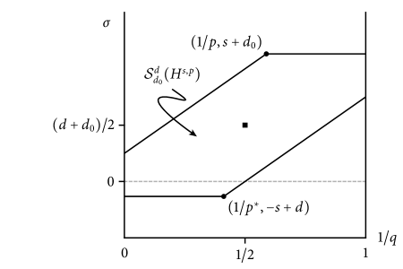
Refer to caption — Figure 1: The region $\mathcal{S}_{d_{0}}^{d}(H^{s,p})$ for $n=3$ , $d=2$ , $d_{0}=0$ , $p=1.7$ and $s=\frac{n}{p}+\frac{1}{2}$ .

The second condition of (2.6) is a restriction on the Lebesgue regularity of $(\sigma,q)$ and it is helpful to visualize $\mathcal{S}^{d}_{d_{0}}(H^{s,p})$ after making the transformation $q\mapsto 1/q$ since sets of constant Lebesgue regularity then appear as straight lines with slope $1/n$ as in Figure 1.

For any particular collection of parameters, it may be that $\mathcal{S}^{d}_{d_{0}}(H^{s,p})$ is empty. The following result establishes when the set is nonempty and hence when an operator of class $\mathcal{L}_{d_{0}}^{d}(H^{s,p};\Omega)$ has a suitable collection of Bessel potential spaces to act on.

Lemma 2.8.

Suppose $1<p<\infty$ , $s\in\mathbb{R}$ and $d,d_{0}\in\mathbb{Z}_{\geq 0}$ with $d\geq d_{0}$ . Then $\mathcal{S}_{d_{0}}^{d}(H^{s,p})$ is nonempty if and only if

	$\displaystyle s$	$\displaystyle\geq(d-d_{0})/2\text{, and}$		(2.7)
	$\displaystyle\frac{1}{p}-\frac{s}{n}$	$\displaystyle\leq\frac{1}{2}-\frac{(d-d_{0})/2}{n}.$		(2.8)

If $S_{d_{0}}^{d}(H^{s,p})$ is non-empty then it contains $(s+d_{0},p)$ , $(d-s,p^{*})$ , and $((d+d_{0})/2,2)$ . Moreover, if $(\sigma,q)\in\mathcal{S}_{d_{0}}^{d}(H^{s,p})$ , then we have the continuous inclusions of Fréchet spaces

H^{s+d_{0},p}_{\rm loc}(\mathbb{R}^{n})\subseteq H^{\sigma,q}_{\rm loc}(\mathbb{R}^{n})\subseteq H^{d-s,p^{*}}_{\rm loc}(\mathbb{R}^{n}).

(2.9)

Proof.

The intervals in (2.6) defining $\mathcal{S}_{d_{0}}^{d}(H^{s,p})$ are non-empty if and only if $s\geq(d-d_{0})/2$ and

\frac{1}{p}-\frac{s+d_{0}}{n}\leq 1-\frac{1}{p}-\frac{d-s}{n},

which is equivalent to inequality (2.8). Moreover, if these intervals are nonempty, then $(s+d_{0},p)$ and $(d-s,p^{*})$ evidently belong to $\mathcal{S}_{d_{0}}^{d}(H^{s,p})$ . To show that $(\sigma,q)=((d+d_{0})/2,2)\in\mathcal{S}_{d_{0}}^{d}(H^{s,p})$ whenever this set is nonempty, define

\frac{1}{r_{1}}=\frac{1}{p}-\frac{s+d_{0}}{n},\qquad\frac{1}{r_{2}}=\frac{1}{p^{*}}-\frac{d-s}{n},\quad\text{and}\quad\frac{1}{r}=\frac{1}{2}-\frac{(d+d_{0})/2}{n}.

Then $((d+d_{0})/2,2)\in\mathcal{S}_{d_{0}}^{d}(H^{s,p})$ so long as

d-s\leq\frac{d+d_{0}}{2}\leq s+d_{0}

(2.10)

and

\frac{1}{r_{1}}\leq\frac{1}{r}\leq\frac{1}{r_{2}}.

(2.11)

Since $\mathcal{S}_{d_{0}}^{d}(H^{s,p})$ is nonempty, $d-s\leq s+d_{0}$ and $1/r_{1}\leq 1/r_{2}$ . Inequalities (2.10) and (2.11) are then consequences of the observations

\frac{d+d_{0}}{2}=\frac{1}{2}\left[(d-s)+(s+d_{0})\right]

and

\frac{1}{r}=\frac{1}{2}\left(\frac{1}{r}_{1}+\frac{1}{r}_{2}\right).

Finally, recall that $H^{s_{1},p_{1}}_{\rm loc}(\mathbb{R}^{n})$ embeds continuously in $H^{s_{2},p_{2}}_{\rm loc}(\mathbb{R}^{n})$ if $s_{1}\geq s_{2}$ and if

\frac{1}{p_{1}}-\frac{s_{1}}{n}\leq\frac{1}{p_{2}}-\frac{s_{2}}{n}.

So conditions (2.6) ensure that if $(\sigma,q)\in\mathcal{S}_{d_{0}}^{d}(H^{s,p})$ then we have the continuous inclusions (2.9). ∎

The indices $(s+d_{0},p)$ and $(d-s,p^{*})$ correspond to the most regular and least regular spaces an operator in $\mathcal{L}_{d_{0}}^{d}(H^{s,p};\Omega)$ can naturally act on; indices $(\sigma,q)\in\mathcal{S}_{d_{0}}^{d}(H^{s,p})$ yield spaces $H^{\sigma,q}_{\rm loc}(\mathbb{R}^{n})$ that lie intermediate between the two extreme spaces $H^{s+d_{0},p}_{\rm loc}(\mathbb{R}^{n})$ and $H^{d-s,p^{*}}_{\rm loc}(\mathbb{R}^{n})$ . Indeed, one interpretation of Lemma 2.8 is that $\mathcal{S}^{d}_{d_{0}}(H^{s,p})$ is nonempty exactly when $H^{s+d_{0},p}_{\rm loc}(\mathbb{R}^{n})$ includes $H^{d-s,p^{*}}_{\rm loc}(\mathbb{R}^{n})$ . Alternatively, inequalities (2.7)–(2.8) are exactly the condition that $H^{s,p}_{\rm loc}$ includes $H^{(d+d_{0})/2,2}_{\rm loc}$ , which highlights the importance of this $L^{2}$ -based space. In effect, Lemma 2.8 implies $\mathcal{S}_{d_{0}}^{d}(H^{s,p})$ is nonempty exactly when it contains $((d+d_{0})/2,2)$ . For example, consider the case of a general second-order operator, so $d=2$ and $d_{0}=0$ . Then $\mathcal{S}_{0}^{2}(H^{s,p})$ is non-empty when $H^{s,p}_{\rm loc}(\mathbb{R}^{n})$ contains $H^{1,2}_{\rm loc}(\mathbb{R}^{n})$ , the natural $L^{2}$ -based space for a weak existence theory. See also Figure 1, where the key $L^{2}$ -based space appears as a small square.

In addition to the mapping properties of $L$ described in Proposition 2.6 we require an analogous result for the commutator of $L$ with a smooth cutoff function $\phi$ .

Lemma 2.9.

Let $\Omega$ be a bounded open subset of $\mathbb{R}^{n}$ . Suppose $1<p,q<\infty$ , $s>n/p$ , $\sigma\in\mathbb{R}$ and $d,d_{0}\in\mathbb{Z}_{\geq 0}$ with $d\geq d_{0}$ . Let $L$ be an operator of class $\mathcal{L}_{d_{0}}^{d}(H^{s,p};\Omega)$ and let $\phi\in\mathcal{D}(\Omega)$ . Then $[L,\phi]$ extends from a map $C^{\infty}(\overline{\Omega})\mapsto\mathcal{D}^{\prime}(\Omega)$ to a continuous linear map $H^{\sigma,q}(\Omega)\mapsto H^{\sigma-d+1,q}(\Omega)$ so long as $(\sigma+1,q)\in\mathcal{S}^{d}_{d_{0}}(H^{s,p})$ . Moreover, if $d_{0}=0$ , the same result holds if $(\sigma,q)\in\mathcal{S}^{d}_{0}(H^{s,p})$ .

Proof.

Suppose $u\in H^{\sigma,q}(\Omega)$ . A term of $[L,\phi]u$ has the form

a^{\alpha}\partial_{\beta}\phi\partial_{\gamma}u

where $a^{\alpha}\in H^{s-d+|\alpha|,p}$ and where $\max(1,d_{0})\leq|\alpha|\leq d$ and $|\gamma|\leq|\alpha|-1$ . The result in the case of general $d_{0}$ follows from a direct computation using these facts along with Theorem 2.5.

If $d_{0}=0$ , we can improve the result as follows. Let $\hat{L}$ be $L$ with its zero-order term removed, so $\hat{L}\in\mathcal{L}_{1}^{d}(H^{s,p};\Omega)$ . Then $[L,\phi]=[\hat{L},\phi]$ and using the result just proved we find that the commutator $[L,\phi]$ maps $H^{\sigma,q}(\Omega)\to H^{\sigma-d+1,a}(\Omega)$ so long as $(\sigma+1,q)\in\mathcal{S}^{d}_{1}(H^{s,p})$ . But a routine computation shows that this condition is equivalent to $(\sigma,q)\in\mathcal{S}^{d-1}_{0}(H^{s,p})$ and the claimed improvement follows since $S^{d-1}_{0}(H^{s,p})\supset S^{d}_{0}(H^{s,p})$ . ∎

2.2 Rescaling estimates

For a Schwartz function $u$ let $u_{\{r\}}(x)=u(rx)$ . This rescaling operation extends to general tempered distributions by continuity and duality arguments, and we use the same notation when $u$ is a distribution. When $m$ is a non-negative integer, it is easy to see that $u\mapsto u_{\{r\}}$ is a continuous automorphism of $H^{m,p}(\mathbb{R}^{n})$ for all $1<p<\infty$ . The same holds for $H^{s,p}(\mathbb{R}^{n})$ for $s>0$ by interpolation, and for $s<0$ by an elementary duality argument.

In this section, we prove two principal estimates for the norms of rescaling operators, with bounds depending on $r$ along with the parameters of the function space being acted on. First, we have Proposition 2.10, which establishes the desired estimates for functions with integer-order differentiability. Then, using interpolation, we generalize the estimates to non-integer differentiability at the penalty of a mild loss of sharpness; this is the content of Proposition 2.17, which is the main result of this section. In fact, one can recover the sharpness using more sophisticated tools from Littlewood-Paley theory, and indeed we do for the broader class of Triebel-Lizorkin spaces in Section 3.2. Nevertheless, the less-than optimal estimates of Proposition 2.17 are sufficient to establish local elliptic regularity in the context of Bessel potential function spaces, and it permits a proof using only a minimal set of tools.

Proposition 2.10.

Suppose $1<p<\infty$ , $m\in\mathbb{Z}$ and that $\chi$ is a Schwartz function on $\mathbb{R}^{n}$ . There exists a constant $\alpha\in\mathbb{R}$ such that for all $0<r\leq 1$ and all $u\in H^{m,p}(\mathbb{R}^{n})$

||\chi u_{\{r\}}||_{H^{m,p}(\mathbb{R}^{n})}\lesssim r^{\alpha}||u||_{H^{m,p}(\mathbb{R}^{n})}.

(2.12)

Specifically:

1.

Inequality (2.12) holds with

$\alpha=\min\left(m-\frac{n}{p},0\right)$

unless $m-n/p=0$ , in which case it holds for any choice of $\alpha<0$ , with implicit constant depending on $\alpha$ .
2.

If $m>n/p$ (in which case functions in $H^{m,p}(\mathbb{R}^{n})$ are Hölder continuous) and if $u(0)=0$ , then inequality (2.12) holds with

$\alpha=\min\left(m-\frac{n}{p},1\right)$

unless $m-n/p=1$ , in which case it holds for any choice of $\alpha<1$ , with implicit constant depending on $\alpha$ .

Proposition 2.10 is established in the following sequence of elementary results which treat specific subcases and supporting lemmas. Specifically, it is an immediate consequence of Corollary 2.13, Lemma 2.14 and Corollary 2.16 below. In applications, $\chi$ in Proposition 2.10 will be compactly supported and we are effectively interested in rescaling $u$ from a ball of radius $r<1$ up to a ball of fixed radius. Derivatives are dampened under this operation, and the role of $\chi$ is to control the zero-frequency terms; without the cutoff function, for all $m>0$ the optimal scaling would be $\alpha=-n/p$ instead.

We begin in the easier setting $m\leq 0$ , in which case it turns out that the the cutoff function plays no role. When $m=0$ , we have the following consequence of the change of variables formula that the $L^{p}$ norm has straightforward scaling behavior for all $r>0$ .

Lemma 2.11.

Suppose $1<p<\infty$ , $r>0$ , and $u\in L^{p}(\mathbb{R}^{n})$ . Then

||u_{\{r\}}||_{L^{p}(\mathbb{R}^{n})}=||u||_{L^{p}(\mathbb{R}^{n})}r^{-n/p}.

Turning to the case $m<0$ in Proposition 2.10, the proof proceeds via a duality argument, for which we need the following result concerning rescaling $H^{k,p}(\mathbb{R}^{n})$ for $k>0$ with $r>1$ (rather than $r\leq 1$ ).

Lemma 2.12.

Suppose $1<p<\infty$ and $k\in\mathbb{Z}_{\geq 0}$ . For all $r\geq 1$ and all $u\in H^{k,p}(\mathbb{R}^{n})$ ,

||u_{\{r\}}||_{H^{k,p}(\mathbb{R}^{n})}\lesssim||u||_{H^{k,p}(\mathbb{R}^{n})}r^{m-\frac{n}{p}}.

(2.13)

Proof.

Lemma 2.11, the Gagliardo-Nirenberg-Sobolev inequality and the fact that $r\geq 1$ imply

	$\displaystyle\|\|u_{\{r\}}\|\|_{H^{k,p}(\mathbb{R}^{n})}$	$\displaystyle\lesssim\|\|u_{\{r\}}\|\|_{L^{p}(\mathbb{R}^{n})}+\sum_{\|\alpha\|=k}\|\|\nabla^{\alpha}u_{\{r\}}\|\|_{L^{p}(\mathbb{R}^{n})}$
		$\displaystyle=r^{-\frac{n}{p}}\|\|u\|\|_{L^{p}(\mathbb{R}^{n})}+r^{k}\sum_{\|\alpha\|=k}\|\|(\nabla^{\alpha}u)_{\{r\}}\|\|_{L^{p}(\mathbb{R}^{n})}$
		$\displaystyle=r^{-\frac{n}{p}}\|\|u\|\|_{L^{p}(\mathbb{R}^{n})}+r^{k-\frac{n}{p}}\sum_{\|\alpha\|=k}\|\|(\nabla^{\alpha}u)\|\|_{L^{p}(\mathbb{R}^{n})})$
		$\displaystyle\lesssim r^{k-\frac{n}{p}}\|\|u\|\|_{H^{k,p}(\mathbb{R}^{n})}.$

∎

The following corollary follows from duality from Lemma 2.12.

Corollary 2.13.

Suppose $1<p<\infty$ and $m\in\mathbb{Z}_{\leq 0}$ . For all $0<r\leq 1$ and all $u\in H^{m,p}(\mathbb{R}^{n})$

||u_{\{r\}}||_{H^{m,p}(\mathbb{R}^{n})}\lesssim r^{m-\frac{n}{p}}||u||_{H^{m,p}(\mathbb{R}^{n})}.

Proof.

Using a density argument it is enough to establish the result when $u$ is smooth and compactly supported. For any test function $\phi$ ,

$\displaystyle\|\left<u_{\{r\}},\phi\right>\|$	$\displaystyle=\left\|\int_{\mathbb{R}^{n}}u(rx)\phi(x)\;dx\right\|$	(2.14)
	$\displaystyle=r^{-n}\left\|\int_{\mathbb{R}^{n}}u(y)\phi(y/r)\;dy\right\|$
	$\displaystyle\leq r^{-n}\|\|u\|\|_{H^{m,p}(\mathbb{R}^{n})}\|\|\phi_{{\{1/r\}}}\|\|_{H^{-m,p^{*}}(\mathbb{R}^{n})}.$

Since $-m\geq 0$ and since $1/r\geq 1$ , Lemma 2.12 implies

||\phi_{{\{1/r\}}}||_{H^{-m,p^{*}}(\mathbb{R}^{n})}\lesssim r^{m+\frac{n}{p^{*}}}||\phi||_{H^{-m,p^{*}}(\mathbb{R}^{n})}

where the implicit constant is independent of $r$ and $u$ . Hence

|\left<u_{\{r\}},\phi\right>|\lesssim||u||_{H^{m,p}(\mathbb{R}^{n})}||\phi||_{H^{-m,p^{*}}(\mathbb{R}^{n})}r^{-n+m+\frac{n}{p^{*}}}=||u||_{H^{m,p}(\mathbb{R}^{n})}||\phi||_{H^{-m,p^{*}}(\mathbb{R}^{n})}r^{m-\frac{n}{p}},

which concludes the proof, noting that $H^{m,p}(\mathbb{R}^{n})$ is the dual space of $H^{-m,p^{*}}(\mathbb{R}^{n})$ . ∎

Corollary 2.13 implies Proposition 2.10 in the case $m\leq 0$ , for if $\chi$ is a Schwartz function $||\chi u||_{H^{m,p}(\mathbb{R}^{n})}\lesssim||u||_{H^{m,p}(\mathbb{R}^{n})}.$ We now turn to the more involved case of Proposition 2.10, $m>0$ .

Lemma 2.14.

Suppose $1<p<\infty$ , $m\in\mathbb{N}$ and that $\chi$ is a Schwartz function on $\mathbb{R}^{n}$ . There exists $\alpha\in\mathbb{R}$ such that for all $1<r\leq 1$ and all $u\in H^{m,p}(\mathbb{R}^{n})$

||u_{\{r\}}||_{H^{m,p}(\mathbb{R}^{n})}\lesssim r^{\alpha}||u||_{H^{m,p}(\mathbb{R}^{n})}.

(2.15)

Specifically, we can take $\alpha=\min(0,m-n/p)$ in inequality (2.15) unless $m-n/p=0$ , in which case inequality (2.15) holds for any choice of $\alpha<0$ and the implicit constant depends on $\alpha$ .

Proof.

Repeated applications of the Gagliardo-Nirenberg-Sobolev inequality imply

||\chi u_{\{r\}}||_{H^{m,p}(\mathbb{R}^{n})}\lesssim||\chi u_{\{r\}}||_{L^{p}(\mathbb{R}^{n})}+||\nabla^{m}u_{\{r\}}||_{L^{p}(\mathbb{R}^{n})}

(2.16)

where the implicit constant depends on $\chi$ ; since $\chi$ is fixed the explicit dependence is unimportant.

The second term on the right-hand side of equation (2.16) is easy to estimate. Using the identity $\nabla^{m}u_{\{r\}}=r^{m}(\nabla^{m}u)_{\{r\}}$ Lemma 2.11 we find

||\nabla^{m}u_{\{r\}}||_{L^{p}(\mathbb{R}^{n})}\lesssim r^{m-n/p}||\nabla^{m}u||_{L^{p}(\mathbb{R}^{m})}\leq r^{m-n/p}||u||_{H^{m,p}(\mathbb{R}^{n})}.

Turning to the low order term, first consider the case $m>n/p$ . Sobolev imbedding implies $u\in L^{\infty}(\mathbb{R}^{n})$ and

	$\displaystyle\|\|\chi u_{\{r\}}\|\|_{L^{p}(\mathbb{R}^{n})}\leq\|\|\chi\|\|_{L^{p}(\mathbb{R}^{n})}\|\|u_{\{r\}}\|\|_{L^{\infty}(\mathbb{R}^{n})}$	$\displaystyle=\|\|\chi\|\|_{L^{p}(\mathbb{R}^{n})}\|\|u\|\|_{L^{\infty}(\mathbb{R}^{n})}$
		$\displaystyle\lesssim\|\|u\|\|_{H^{m,p}(\mathbb{R}^{n})}=r^{\min(0,m-n/p)}\|\|u\|\|_{H^{m,p}(\mathbb{R}^{n})}$

Now suppose $m<n/p$ . Then Sobolev embedding implies $u\in L^{q}(\mathbb{R}^{n})$ where

\frac{1}{q}=\frac{1}{p}-\frac{m}{n}.

Hölder’s inequality, the fact that $\chi$ lies in every Lebesgue space, and Lemma 2.11 imply

	$\displaystyle\|\|\chi u_{\{r\}}\|\|_{L^{p}(\mathbb{R}^{n}))}\lesssim\|\|u_{\{r\}}\|\|_{L^{q}(\mathbb{R}^{n})}$	$\displaystyle\leq r^{-n/q}\|\|u\|\|_{L^{q}(\mathbb{R}^{n})}$
		$\displaystyle=r^{m-n/p}\|\|u\|\|_{L^{q}(\mathbb{R}^{n})}\lesssim r^{m-n/p}\|\|u\|\|_{H^{m,p}(\mathbb{R}^{n})}=r^{\min(m-n/p,0)}\|\|u\|\|_{H^{m,p}(\mathbb{R}^{n})}.$

When $m=n/p$ we use the marginal case of Sobolev embedding and an argument similar to the above to conclude

||\chi u_{\{r\}}||_{L^{p}(\mathbb{R}^{n})}\lesssim r^{-n/q}||u||_{H^{m,p}(\mathbb{R}^{n})}

for any $q\geq p$ . Taking $q$ sufficiently large we find inequality (2.15) holds for any choice of $\alpha<0$ . ∎

Lemma 2.14 completes the proof of part (1) of Proposition 2.10, and the following two results establish part (2).

Lemma 2.15.

Let $\chi$ be a Schwartz function on $\mathbb{R}^{n}$ and let $\alpha\in[0,1]$ . For all $0<r\leq 1$ and all $u\in C^{0,\alpha}(\mathbb{R}^{n})$ with $u(0)=0$ ,

||\chi u_{\{r\}}||_{L^{p}(\mathbb{R}^{n})}\lesssim||u||_{C^{0,\alpha}(\mathbb{R}^{n})}r^{\alpha}.

Proof.

We divide $\mathbb{R}^{n}$ into three regions: the ball $B_{1}(0)$ , the annulus $A=B_{1/r}(0)\setminus B_{1}(0)$ and the exterior region $E=\mathbb{R}^{n}\setminus B_{1/r}(0)$ . On the unit ball, since $u(0)=0$ ,

||\chi u_{\{r\}}||_{L^{p}(B_{1}(0))}\lesssim||\chi||_{L^{\infty}(\mathbb{R}^{n})}||u||_{C^{0,\alpha}(B_{1}(0))}r^{\alpha}.

To obtain the remainder of the estimate, pick a constant $B>0$ such that $|\chi(x)|\leq B|x|^{-(n+1)/p-\alpha}$ for all $x\in\mathbb{R}^{n}$ with $|x|\geq 1$ . Then, letting $C_{n}$ be the volume of the unit $n-1$ sphere, we find on the annulus $A$ ,

	$\displaystyle\int_{A}\chi^{p}u_{\{r\}}^{p}$	$\displaystyle\leq C_{n}\int_{1}^{1/r}B^{p}s^{-n-1-\alpha p}\|\|u\|\|_{C^{0,\alpha}(\mathbb{R}^{n})}^{p}(rs)^{\alpha p}s^{n-1}\;ds$		(2.17)
		$\displaystyle\leq C_{n}B^{p}\|\|u\|\|_{C^{0,\alpha}(\mathbb{R}^{n})}^{p}r^{p\alpha}\int_{1}^{1/r}s^{-2}\;ds\leq C_{n}B^{p}\|\|u\|\|_{C^{0,\alpha}(\mathbb{R}^{n})}^{p}r^{p\alpha}.$		(2.17)

Taking $p^{\rm th}$ roots establishes the desired estimate on $A$ .

Finally, for the exterior region we have

\int_{E}|\chi u_{\{r\}}|^{p}\leq C_{n}B^{p}||u||_{C_{0,\alpha}(\mathbb{R}^{n})}^{p}\int_{1/r}^{\infty}s^{-n-1-\alpha p}s^{n-1}\;ds=C_{n}B^{p}||u||_{C^{0,\alpha}(\mathbb{R}^{n})}^{p}\frac{1}{1+\alpha p}r^{1+\alpha p}

which completes the proof. ∎

Corollary 2.16.

Let $\chi$ be a Schwartz function on $\mathbb{R}^{n}$ . Suppose $1<p<\infty$ and $m\in\mathbb{N}$ with $m>n/p$ . There exists $\alpha\in\mathbb{R}$ such that for all $0<r\leq 1$ and all $u\in H^{m,p}(\mathbb{R}^{n})$ with $u(0)=0$

||\chi u_{\{r\}}||_{H^{m,p}(\mathbb{R}^{n})}\lesssim r^{\alpha}||u||_{H^{m,p}(\mathbb{R}^{n})}.

(2.18)

Specifically, we can take $\alpha=\min(1,m-n/p)$ in inequality (2.18) unless $m-n/p=1$ , in which case inequality (2.18) holds for any choice of $\alpha<1$ and the implicit constant depends on $\alpha$ .

Proof.

Following the argument of the beginning of the proof of Lemma 2.14 we know that

||\chi u_{\{r\}}||_{H^{m,p}(\mathbb{R}^{n})}\lesssim||\chi u_{\{r\}}||_{L^{p}(\mathbb{R}^{n})}+||\nabla^{m}u_{\{r\}}||_{L^{p}(\mathbb{R}^{n})}

and that $||\nabla^{m}u_{\{r\}}||_{L^{p}(\mathbb{R}^{n})}\lesssim r^{m-n/p}||u||_{H^{s,p}(\mathbb{R}^{n})}$ . Hence it suffices to show

||\chi u_{\{r\}}||_{L^{p}(\mathbb{R}^{n})}\lesssim r^{\min(1,m-n/p)}||u||_{H^{m,p}(\mathbb{R}^{n})}.

Suppose first that $0<m-n/p<1$ . Then $u\in C^{0,\alpha}(\mathbb{R}^{n})$ with $\alpha=m-n/p$ . Since $u(0)=0$ , Lemma 2.15 implies

||\chi u_{\{r\}}||_{L^{p}(\mathbb{R}^{n})}\lesssim||u||_{C^{0,\alpha}(\mathbb{R}^{n})}r^{\alpha}\lesssim||u||_{H^{m,p}(\mathbb{R}^{n})}r^{m-n/p}=||u||_{H^{m,p}(\mathbb{R}^{n})}r^{\min(1,m-n/p)}.

On the other hand, if $m-n/p>1$ then $u$ lies in $C^{0,1}(\mathbb{R}^{n})$ and the same argument shows

||\chi u_{\{r\}}||_{L^{p}(\mathbb{R}^{n})}\lesssim||u||_{H^{m,p}(\mathbb{R}^{n})}r^{1}=||u||_{H^{m,p}(\mathbb{R}^{n})}r^{\min(1,m-n/p)}

The result in the marginal case $m-n/p=1$ follows from a similar argument using the fact that $H^{m,p}(\mathbb{R}^{n})$ embeds into $C^{0,\alpha}(\mathbb{R}^{n})$ for any $\alpha\in(0,1)$ . ∎

Having now established Proposition 2.10, we turn to its generalization to non-integer orders of differentiability. In fact, one can show that the statement of Proposition 2.10 generalizes without change, other than replacing $m\in\mathbb{Z}$ with $s\in\mathbb{R}$ ; see Proposition 3.10 which establishes an extension of this fact to the broader class of Triebel-Lizorkin spaces. The following result is mildly weaker, but is easier to prove and is sufficient for our application establishing local elliptic regularity. The key difference is that the equal sign in the definition of the exponent $\alpha$ in parts (1) and (2) of Proposition 2.10 has been replaced with a strict inequality.

Proposition 2.17.

Suppose $1<p<\infty$ , $s\in\mathbb{R}$ and $\chi$ is a Schwartz function on $\mathbb{R}^{n}$ . There exists $\alpha\in\mathbb{R}$ such that for all $0<r\leq 1$ and all $u\in H^{s,p}(\mathbb{R}^{n})$ ,

||\chi u_{\{r\}}||_{H^{s,p}(\mathbb{R}^{n})}\lesssim r^{\alpha}||u||_{H^{s,p}(\mathbb{R}^{n})}.

(2.19)

In particular:

1.

Inequality (2.19) holds with any

$\alpha<\min\left(s-\frac{n}{p},0\right)$

with implicit constant depending on $\alpha$ .
2.

If $s>n/p$ and $u(0)=0$ then inequality (2.19) holds with any

$\alpha<\min\left(s-\frac{n}{p},1\right)$

with implicit constant depending on $\alpha$ .

Proof.

We divide the tuples $(s,1/p)$ in $\mathbb{R}\times(0,1)$ into the following regions (see Figure 2):

$\mathcal{A}$ :

$s\leq n-1$ , $0<1/p<1$ , $s-n/p<0$ ,
$\mathcal{B}$ :

$s\geq 1$ , $0<1/p<1$ , $s-n/p>0$ ,
$\mathcal{C}$ :

$s<1$ , $s-n/p\geq 0$ ,
$\mathcal{D}$ :

$s>n-1$ , $s-n/p\leq 0$ ,
$\mathcal{E}$ :

$1\leq s\leq n-1$ , $s-n/p=0$ .

Suppose $(s,1/p)\in\mathcal{A}$ and for the moment assume $s\geq 0$ . If $s$ is an integer, the result follows from Proposition 2.10 so we can assume $0<s<n-1$ . There exist $1/p_{0},1/p_{1}\in(0,1)$ such that $(s,1/p)$ lies on the line joining $(0,1/p_{0})$ and $(n-1,1/p_{1})$ . That is,

(s,1/p)=(1-\theta)(0,1/p_{0})+\theta(n-1,1/p_{1})

for some $\theta\in(0,1)$ . Since $H^{s,p}(\mathbb{R}^{n})=[H^{0,p_{0}}(\mathbb{R}^{n}),H^{n-1,p_{1}}(\mathbb{R}^{n})]_{\theta}$ we conclude from Proposition 2.10 and interpolation applied to the map $u\mapsto\chi u_{\{r\}}$ that

||\chi u_{\{r\}}||_{H^{s,p}(\mathbb{R}^{n})}\lesssim(r^{-n/p_{0}})^{1-\theta}(r^{n-1-n/p_{1}})^{\theta}||u||_{H^{s,p}(\mathbb{R}^{n})}=r^{s-n/p}||u||_{H^{s,p}(\mathbb{R}^{n})}.

Replacing Proposition 2.10 with Corollary 2.13, the same technique works in region $\mathcal{A}$ if $s<0$ and indeed the argument is simpler since we can select $p_{0}=p_{1}=p$ .

If $(s,1/p)\in\mathcal{B}$ and $s$ is an integer then Proposition 2.10 implies inequality (2.12) holds with $\alpha=0$ . When $s$ is not an integer we can interpolate between $(\lfloor s\rfloor,1/p_{1})$ and $(\lceil s\rceil,1/p_{2})$ for appropriate choices of $p_{1}$ and $p_{2}$ to obtain the same result.

Next, suppose $(s,1/p)$ lies in the triangular region $\mathcal{C}$ , so $n/p<s<1$ . Consider any $\sigma$ with $0<\sigma<n/p$ , so $\sigma<s<1$ as well. Then

H^{s,p}(\mathbb{R}^{n})=[H^{\sigma,p}(\mathbb{R}^{n}),H^{1,p}(\mathbb{R}^{n})]_{\theta}

with $\theta=(s-\sigma)/(1-\sigma)\in(0,1)$ . From interpolation we find

||\chi u_{\{r\}}||_{H^{s,p}(\mathbb{R}^{n})}\lesssim(r^{\sigma-n/p})^{1-\theta}||u||_{H^{s,p}(\mathbb{R}^{n})}.

Noting that $1-\theta\to(1-s)/(1-n/p)<\infty$ as $\sigma\to n/p$ we can take $\sigma$ as close to $n/p$ from below as we please to conclude that inequality (2.19) holds with any fixed choice of $\alpha<0$ . Note that this interpolation, and the one to follow for region $\mathcal{D}$ , is the source of the loss of sharpness of the current proposition.

In the region $\mathcal{D}$ the argument is similar to the argument for region $\mathcal{C}$ ; we now interpolate between a point with $s=n-1$ and a point with $s>n/p$ in region $\mathcal{A}$ taken arbitrarily close to the line $s=n/p$ . On the line segment $\mathcal{E}$ the proof follows by interpolating between a point in region $\mathcal{A}$ and a point region $\mathcal{B}$ taken arbitrarily close to the line segment. This completes the proof of part (1).

The proof of part (2) is proved in a completely analogous way with the main division now occurring on the line $s=n/p+1$ . Given the careful proof of part (1) we omit the details. ∎

2.3 Interior elliptic estimates

This section contains our principal elliptic regularity results, which are established in two steps. First, Proposition 2.20 shows that if an operator is elliptic at a single point, then elliptic regularity can be established for functions that are supported in a sufficiently small neighborhood near the point. The rescaling estimates of the previous section, along with a parametrix construction, are the key tools needed at this first stage. Theorem 3.21 then builds on Proposition 2.20 to obtain full interior regularity for elliptic operators using a partition of unity argument along with a bootstrap. The commutator estimates of Lemma 2.9 are the key technical used at this second stage.

Definition 2.18.

Let $\Omega$ be an open subset of $\mathbb{R}^{n}$ . Suppose $1<p<\infty$ and $s>n/p$ . An operator

\sum_{|\alpha|\leq d}a^{\alpha}\partial_{\alpha}

of class $\mathcal{L}_{d_{0}}^{d}(H^{s,p};\Omega)$ is elliptic at $x_{0}\in\Omega$ if for every $\xi\in\mathbb{R}^{n}\setminus\{0\}$

\sum_{|\alpha|=d}a^{\alpha}(x_{0})\xi^{\alpha}\in\mathbb{R}^{k\times k}

is non-singular, where $\xi^{\alpha}=\xi^{\alpha_{1}}\cdots\xi^{\alpha_{d}}$ .

We have the following standard parametrix construction for homogeneous, constant coefficient elliptic operators.

Lemma 2.19.

Suppose $L=\sum_{|\alpha|=d}a^{\alpha}\partial_{\alpha}$ is a constant coefficient elliptic differential operator. There exists maps $Q$ and $T$ acting on tempered distributions supported on $B_{R}(0)$ such that

•

$Q:H^{s-d,p}(\mathbb{R}^{n})\to H^{s,p}(\mathbb{R}^{n})$ is is continuous for all $s\in\mathbb{R}$ and $1<p<\infty$ ,
•

$T:H^{s_{1},p}(\mathbb{R}^{n})\to H^{s_{2},p}(\mathbb{R}^{n})$ is continuous for all $s_{1},s_{2}\in\mathbb{R}$ and $1<p<\infty$ ,
•

$QLu=u+Tu$ for all tempered distributions $u$ .

Proof.

Let $\chi$ be a smooth, compactly supported cutoff function that equals 1 in a neighborhood of zero. Define the parametrix $Q$ on tempered distributions by $Qu=\mathcal{F}^{-1}(1-\chi(\xi))(a^{\alpha}\xi^{\alpha})^{-1}\mathcal{F}$ , where $\mathcal{F}$ is the Fourier transform. Similarly, let $T$ be the smoothing map $Tu=\mathcal{F}^{-1}\chi(\xi)\mathcal{F}$ . A computation shows $QLu=u+Tu$ for all tempered distributions.

Setting $\left<\xi\right>=\sqrt{1+|\xi|^{2}}$ , the claimed continuity properties of $Q$ follows from factoring the multiplier as

\left[(1-\chi(\xi))(a^{\alpha}\xi^{\alpha})^{-1}\left<\xi\right>^{d}\right]\left<\xi\right>^{-d}

The continuity of the multiplier operator determined by the the first factor follows from the Mikhlin multiplier theorem whereas the second factor is handled by the definition of Bessel potential spaces.

The smoothing map $T$ has a compactly supported multiplier and its continuity properties follow from the same arguments as above, without restriction on the gain in derivatives. ∎

We now establish Proposition 2.20, the regularity result for functions supported in a sufficiently small region near a point where an operator is elliptic. The statement of this proposition requires notation for function spaces associated with compactly supported functions on a bounded open set $\Omega$ , and there are two natural classes of spaces one can work with. The first is the closure of $\mathcal{D}(\Omega)$ in $H^{s,p}(\Omega)$ . We find it more convenient to take the closure of $\mathcal{D}(\Omega)$ in $H^{s,p}(\mathbb{R}^{n})$ instead; following the notation of [Mc00] we denote this latter space by $\widetilde{H}^{s,p}(\Omega)$ . An element in $\widetilde{H}^{s,p}(\Omega)$ is, by definition, an element of $H^{s,p}(\mathbb{R}^{n})$ and it is easy to see that it has support in $\overline{\Omega}$ . Moreover, if $u\in H^{s,p}(\Omega)$ has support contained in a compact set $V\subseteq\Omega$ , an easy argument using a cutoff function that equals 1 on $V$ and vanishes outside $\Omega$ shows that there exists a unique $\tilde{u}\in\widetilde{H}^{s,p}(\Omega)$ with $\tilde{u}|_{\Omega}=u$ , and indeed one has the estimate $||\tilde{u}||_{\tilde{H}^{s,p}(\Omega)}\lesssim||u||_{H^{s,p}(\Omega)}$ with implicit constant depending on $V$ . Following standard practice we informally identify $u$ with its zero extension $\tilde{u}$ .

Proposition 2.20.

Let $\Omega\subset\mathbb{R}^{n}$ be a bounded open set. Suppose $s\in\mathbb{R}$ , $1<p<\infty$ , $d,d_{0}\in\mathbb{Z}_{\geq 0}$ with $d_{0}\leq d$ , that $s>n/p$ , and that these parameters satisfy inequalities (2.7)–(2.8) of Lemma 2.8 and hence $\mathcal{S}_{d_{0}}^{d}(H^{s,p})\neq\emptyset$ . Suppose additionally that $L=\sum_{|\alpha|\leq d}a^{\alpha}\partial_{\alpha}$ is a differential operator of class $\mathcal{L}_{d_{0}}^{d}(H^{s,p};\Omega)$ and that for some $x\in\Omega$ that

L_{0}=\sum_{|\alpha|=m}a^{\alpha}(x)\partial_{\alpha}

is elliptic. Given $(\sigma,q)\in\mathcal{S}_{d_{0}}^{d}(H^{s,p})$ there exists $r>0$ such that $\overline{B_{r}(x)}\subset\Omega$ and such that if

	$\displaystyle u$	$\displaystyle\in\widetilde{H}^{d-s,p^{*}}(B_{r}(x))\quad\text{and}$
	$\displaystyle Lu$	$\displaystyle\in H^{\sigma-d,q}(\Omega)$

then $u\in H^{\sigma,q}(\Omega)$ and

||u||_{H^{\sigma,q}(\Omega)}\lesssim||Lu||_{H^{\sigma-d,q}(\Omega)}+||u||_{H^{d-s-1,p^{*}}(\Omega)}

(2.20)

with implicit constant independent of $u$ but depending on all other parameters.

Proof.

It suffices to prove the result assuming $x=0$ and that $B_{1}(0)\subset\Omega$ . From the definition of Bessel potential spaces on bounded domains, we can further assume that the coefficients of $L$ have been extended to all of $\mathbb{R}^{n}$ .

For each $r\in(0,1]$ define

L_{[r]}=L_{0}+B_{[r]}+C_{[r]}

where

	$\displaystyle B_{[r]}$	$\displaystyle=\sum_{\|\alpha\|=d}(a^{\alpha}-a^{\alpha}(0))_{\{r\}}\partial_{\alpha}$		(2.21)
	$\displaystyle C_{[r]}$	$\displaystyle=\sum_{\|\alpha\|<d}r^{d-\|\alpha\|}(a^{\alpha})_{\{r\}}\partial_{\alpha}.$		(2.21)

Suppose $u\in\widetilde{H}^{d-s,p^{*}}(B_{r}(0))$ for some $r<1$ and that $Lu\in H^{\sigma-d,q}(\Omega)$ . Recall that by definition $u\in H^{d-s,p^{*}}(\mathbb{R}^{n})$ . Moreover, $Lu$ is compactly supported in $\Omega$ and hence defines an element of $\widetilde{H}^{\sigma-d,q}(\Omega)\subset H^{\sigma-d,q}(\mathbb{R}^{n})\subset H^{-s,p^{*}}(\mathbb{R}^{n})$ . In particular, we can treat $u$ and $Lu$ as distributions on $\mathbb{R}^{n}$ and a short computation shows $u_{\{r\}}$ satisfies

L_{0}u_{\{r\}}+B_{[r]}u_{\{r\}}+C_{[r]}u_{\{r\}}=r^{d}(Lu)_{\{r\}}

as an equation in $H^{-s,p^{*}}(\mathbb{R}^{n})$ .

Pick a cutoff function $\chi$ that equals $1$ on a neighborhood of $\overline{B_{1}(0)}$ . Since $u_{\{r\}}$ is supported on $\overline{B_{1}(0)}$ ,

L_{0}u_{\{r\}}+\chi B_{[r]}u_{\{r\}}+\chi C_{[r]}u_{\{r\}}=r^{d}(Lu)_{\{r\}}

(2.22)

as well.

Let $Q$ and $T$ be the parametrix and smoothing operator for $L_{0}$ from Lemma 2.19. Applying $\chi Q$ to equation (2.22) we have

u_{\{r\}}+\chi Tu_{\{r\}}+\chi Q\circ(\chi(B_{[r]}+C_{[r]}))u_{\{r\}}=r^{d}\chi Q(Lu)_{\{r\}}.

(2.23)

It will be convenient to define $Q^{\prime}=\chi Q$ and $T^{\prime}=\chi T$ , in which case $Q^{\prime}$ has the same continuity properties as in Lemma 2.19 and, using the compact support of $\chi$ , $T^{\prime}$ is a continuous map $H^{s_{1},p_{1}}(\mathbb{R}^{n})\to H^{s_{2},p_{2}}(\mathbb{R}^{n})$ for all choices of $s_{1},s_{2},p_{1},p_{2}$ .

Consider a coefficient of $C_{[r]}$ , $c^{\alpha}=r^{d-|\alpha|}(a^{\alpha})_{\{r\}}\in H^{s-d+|\alpha|,p}(\mathbb{R}^{n})$ . From Proposition 2.17, for any $\epsilon>0$

||\chi c^{\alpha}||_{H^{s-d+|\alpha|,p}(\mathbb{R}^{n})}\lesssim r^{d-|\alpha|}r^{\min\left(s-d+|\alpha|-\frac{n}{p},0\right)-\epsilon}||a^{\alpha}||_{H^{s+d-|\alpha|,p}(\mathbb{R}^{n})}=r^{\min\left(s-\frac{n}{p},d-|\alpha|\right)-\epsilon}||a^{\alpha}||_{H^{s+d-|\alpha|,p}(\mathbb{R}^{n})}.

(2.24)

Similarly, consider a coefficient $b^{\alpha}=(a^{\alpha}-a^{\alpha}(0))_{\{r\}}$ of $B_{[r]}$ . Since $a^{\alpha}\in H^{s,p}(\mathbb{R}^{n})$ when $|\alpha|=d$ , and since $b^{\alpha}(0)=0$ , Proposition 2.17 implies

||\chi b^{\alpha}||_{H^{s,p}(\mathbb{R}^{n})}\lesssim r^{\min\left(s-\frac{n}{p},1\right)-\epsilon}||b^{\alpha}||_{H^{s,p}(\mathbb{R}^{n})}.

(2.25)

Pick $\epsilon>0$ with $\epsilon<\min\left(s-\frac{n}{p},1\right)$ . Since $d-|\alpha|\geq 1$ in estimate (2.24) it follows that the coefficients of $\chi B_{[r]}$ and $\chi C_{{[r]}}$ converge to zero in the norms indicated on the left-hand sides of inequalities (2.24) and (2.25) as $r\to 0$ . Using the fact that these coefficients are compactly supported in a common bounded open set, a computation using Theorem 2.5 shows that $\chi(B_{[r]}+C_{[r]})$ converges to zero as an operator $H^{\sigma^{\prime},q^{\prime}}(\mathbb{R}^{n})\to H^{\sigma^{\prime}-d,q^{\prime}}(\mathbb{R}^{n})$ as $r\to 0$ for any choice of $(\sigma^{\prime},q^{\prime})\in\mathcal{S}^{d}_{d_{0}}(H^{s,p})$ . Hence we may take $r$ sufficiently small so that $I+Q^{\prime}\circ(\chi(B_{[r]}+C_{[r]}))$ has a continuous inverse $U_{[r]}:H^{s-d,p^{*}}(\mathbb{R}^{n})\rightarrow H^{s-d,p^{*}}(\mathbb{R}^{n})$ that also maps $H^{s+d_{0},p}(\mathbb{R}^{n})\rightarrow H^{s+d_{0},p}(\mathbb{R}^{n})$ and $H^{\sigma,q}(\mathbb{R}^{n})\rightarrow H^{\sigma,q}(\mathbb{R}^{n})$ . Applying $U_{[r]}$ to equation (2.23) we conclude

u_{\{r\}}+U_{[r]}T^{\prime}u_{\{r\}}=r^{d}U_{[r]}Q^{\prime}(Lu)_{\{r\}}

and consequently

$\displaystyle\|\|u_{\{r\}}\|\|_{H^{\sigma,q}(\mathbb{R}^{n})}$	$\displaystyle\lesssim\|\|U_{[r]}T^{\prime}u_{\{r\}}\|\|_{H^{\sigma,q}(\mathbb{R}^{n})}+\|\|U_{[r]}Q^{\prime}(Lu)_{\{r\}}\|\|_{H^{\sigma,q}(\mathbb{R}^{n})}$	(2.26)
	$\displaystyle\lesssim\|\|U_{[r]}T^{\prime}u_{\{r\}}\|\|_{H^{s+d_{0},p}(\mathbb{R}^{n})}+\|\|Q^{\prime}(Lu)_{\{r\}}\|\|_{H^{\sigma,q}(\mathbb{R}^{n})}$
	$\displaystyle\lesssim\|\|u_{\{r\}}\|\|_{H^{d-s-1,p^{*}}(\mathbb{R}^{n})}+\|\|(Lu)_{\{r\}}\|\|_{H^{\sigma-d,q}(\mathbb{R}^{n})}.$

Note that the implicit constants above depend on $r$ , but this dependence is unimportant since the smallness of $r$ has already be chosen. Since rescaling $v\mapsto v_{\{r\}}$ with fixed $r$ is a continuous automorphism of any Bessel potential space on $\mathbb{R}^{n}$ we conclude

||u||_{H^{\sigma,q}(\mathbb{R}^{n})}\lesssim||Lu||_{H^{\sigma-d,q}(\mathbb{R}^{n})}+||u||_{H^{d-s-1,p^{*}}(\mathbb{R}^{n})}.

(2.27)

Estimate (2.20) follows from inequality (2.27) along with the fact that if $v\in H^{\sigma^{\prime},q^{\prime}}(\mathbb{R}^{n})$ for some $(\sigma^{\prime},q^{\prime})$ has support on a fixed $\overline{B_{r}(0)}\subset\Omega$ , then $||v||_{H^{\sigma^{\prime},q^{\prime}}(\Omega)}\sim||v||_{H^{\sigma^{\prime},q^{\prime}}(\mathbb{R}^{n})}$ with implicit constants depending on $r$ . ∎

We now arrive at our main regularity result.

Theorem 2.21.

Let $\Omega$ be a bounded open set in $\mathbb{R}^{n}$ and suppose $s,p,d_{0}$ and $d$ are parameters as in Lemma 2.8 such that $s>n/p$ and such that inequalities (2.7)–(2.8) are satisfied so $\mathcal{S}_{d_{0}}^{d}(H^{s,p})\neq\emptyset$ . Suppose $L$ is of class $\mathcal{L}_{d_{0}}^{d}(H^{s,p};\Omega)$ and is elliptic on $\Omega$ . If $u\in H^{d-s,p^{*}}(\Omega)$ and $Lu\in H^{\sigma-d,q}(\Omega)$ for some $(\sigma,q)\in\mathcal{S}_{d_{0}}^{d}(H^{s,p})$ then for any open set $U$ with $\overline{U}\subseteq\Omega$ , $u\in H^{\sigma,q}(U)$ and

||u||_{H^{\sigma,q}(U)}\lesssim||Lu||_{H^{\sigma-d,q}(\Omega)}+||u||_{H^{d-s-1,p^{*}}(\Omega)}.

(2.28)

Proof.

The proof is a bootstrap that relies on the following main step. We have initially assumed that $u\in H^{d-s,p^{*}}(\Omega)$ so that $L$ can be applied to it, and that $Lu\in H^{\sigma-d,q}(\Omega)$ for some $(\sigma,q)\in\mathcal{S}^{d}_{d_{0}}(H^{s,p})$ . Suppose we know additionally that on some open set $\Omega_{A}$ with $\overline{U}\subset\Omega_{A}\subset\Omega$ that $u\in H^{\sigma_{A},q_{A}}(\Omega_{A})$ for some pair $(\sigma_{A},q_{A})$ such that the commutator result Lemma 2.9 applies. Now consider a target level of regularity $(\sigma_{B},q_{B})$ satisfying the following:

H1:

$\sigma_{B}\leq\sigma$ ,
H2:

$\displaystyle\frac{1}{q}-\frac{\sigma}{n}\leq\frac{1}{q_{B}}-\frac{\sigma_{B}}{n}$ ,
H3:

$\sigma_{B}\leq\sigma_{A}+1$ ,
H4:

$\displaystyle\frac{1}{q_{A}}-\frac{\sigma_{A}+1}{n}\leq\frac{1}{q_{B}}-\frac{\sigma_{B}}{n}$ .

The first two conditions ensure via Sobolev embedding that $H^{\sigma,q}(\Omega)$ is contained in $H^{\sigma_{B},q_{B}}(\Omega)$ and form a hard limit on the target regularity. The second two conditions ensure $H^{\sigma_{B},q_{B}}(\Omega_{A})\supset H^{\sigma_{A}+1,q_{A}}(\Omega_{A})$ and limit the improvement in regularity that can be achieved on a single step of the bootstrap. We claim that under these hypotheses that $u\in H^{\sigma_{B},q_{B}}(\Omega_{B})$ for some open set $\Omega_{B}\subset\Omega_{A}$ such that $\overline{U}\subset\Omega_{B}$ and that we have the estimate

||u||_{H^{\sigma_{B},q_{B}}(\Omega_{B})}\lesssim||Lu||_{H^{\sigma-d,q}(\Omega)}+||u||_{H^{\sigma_{A},q_{A}}(\Omega_{A})}

(2.29)

with implicit constant independent of $u$ .

To establish inequality (2.29) we first select an open set $\Omega_{B}$ with $\overline{U}\subseteq\Omega_{B}\subseteq\overline{\Omega}_{B}\subseteq\Omega_{A}$ . Since $\overline{\Omega_{B}}$ is compact we can select finitely many balls $B_{i}=B_{r_{i}}(x_{i})\subset\Omega_{0}$ that cover $\Omega_{B}$ and such that the conclusion of Proposition 2.20 holds for the pair $(\sigma_{B},q_{B})$ . Using a partition of unity subordinate to the balls $B_{i}$ and $\Omega_{A}\setminus\overline{\Omega}_{B}$ we can find non-negative smooth functions $\phi_{i}$ compactly supported in $B_{i}$ such that $\sum\phi_{i}=1$ on $\Omega_{B}$ .

Consider

L(\phi_{i}u)=\phi_{i}Lu+[L,\phi_{i}]u.

(2.30)

From conditions (H1:)–(H2:) and Sobolev embedding we know

||\phi_{i}Lu||_{H^{\sigma_{B}-d,q_{B}}(\Omega_{B})}\lesssim||Lu||_{H^{\sigma_{B}-d,q_{B}}(\Omega_{B})}\lesssim||Lu||_{H^{\sigma-d,q}(\Omega)}.

(2.31)

Conditions (H3:)–(H4:) allow us to apply Sobolev embedding to the commutator term from equation (2.30) and we have

||[L,\phi_{i}]u||_{H^{\sigma_{B}-d,q_{B}}(B_{i})}\lesssim||[L,\phi_{i}]u||_{H^{\sigma_{A}-d+1,q_{A}}(B_{i})}.

(2.32)

Since we have assumed that $(\sigma_{A},q_{A})$ satisfies the conditions of Lemma 2.9 (i.e., either $(\sigma_{A}+1,q_{A})\in\mathcal{S}^{d}_{d_{0}}(H^{s,p})$ or $d_{0}=0$ and $(\sigma_{A},q_{A})\in\mathcal{S}^{d}_{d_{0}}(H^{s,p})$ ), we have

||[L,\phi_{i}]u||_{H^{\sigma_{A}-d+1,q_{A}}(B_{i})}\lesssim||u||_{H^{\sigma_{A},q_{A}}(B_{i})}\lesssim||u||_{H^{\sigma_{A},q_{A}}(\Omega_{A})}.

(2.33)

Combining inequalities equalities (2.31), (2.32) and (2.32) we find $L(\phi_{i}u)\in H^{\sigma_{B}-d,q_{B}}(B_{i})$ and we conclude from Proposition 2.20 that $\phi_{i}u\in H^{\sigma_{B},q_{B}}(\mathbb{R}^{n})$ and additionally

||\phi_{i}u||_{H^{\sigma_{B},q_{B}}(\Omega_{A})}\lesssim||Lu||_{H^{\sigma,q}(\Omega)}+||u||_{H^{\sigma_{A},q_{A}}(\Omega_{A})}.

Inequality (2.29) now follows from the observation $||\phi_{i}u||_{H^{\sigma_{B},q_{B}}(\Omega_{B})}\lesssim||\phi_{i}u||_{H^{\sigma_{B},q_{B}}(\Omega_{A})}$ and summing on $i$ .

We now describe the bootstrap in the easier case when $d_{0}=0$ , where Lemma 2.9 has the fewest restrictions. The argument begins with $(\sigma_{0},q_{0})=(d-s-1,p^{*})$ and $(\sigma_{1},q_{1})=(d-s,p^{*})$ . Conditions (H1:)–(H2:) are an immediate consequence of the definition of the region $\mathcal{S}^{d}_{0}(H^{s,p})$ and conditions (H3:)–(H4:) are obvious. Moreover, since $(\sigma_{0}+1,q_{0})=(d-s,p^{*})\in\mathcal{S}^{d}_{0}(H^{s,p})$ , Lemma 2.9 applies. Hence all the conditions of the bootstrap step are met and we conclude there is an open set $\Omega_{1}$ with $\overline{U}\subset\Omega_{1}\subset\Omega$ such that

||u||_{H^{d-s,p^{*}}(\Omega_{1})}\lesssim||Lu||_{H^{\sigma,q}(\Omega)}+||u||_{H^{d-s-1,p^{*}}(\Omega)}.

(2.34)

We now iteratively apply the bootstrap step through a finite sequence $(\sigma_{k},q_{k})$ in $S^{d}_{0}(H^{s,p})$ described below that starts at $(s-d,p^{*})$ and terminates at $(\sigma,q)$ . At each step we ensure conditions (H1:)–(H4:) hold and obtain inequalities

||u||_{H^{\sigma_{k+1},q_{k+1}}(\Omega_{k+1})}\lesssim||Lu||_{H^{\sigma,q}(\Omega)}+||u||_{H^{\sigma_{k},q_{k}}(\Omega_{k})}

(2.35)

for a sequence nested open sets $\overline{U}\subset\Omega_{k+1}\subset\Omega_{k}\subset\Omega$ . Because we have assumed that $d_{0}=0$ , and since each $(\sigma_{k},q_{k})\in\mathcal{S}^{d}_{0}(H^{s,p})$ , we are assured that at each step we can use the commutator estimate from Lemma (2.9). Inequality (2.28) follows from chaining together the initial estimate (2.34) with the estimates (2.35) obtained along the bootstrap.

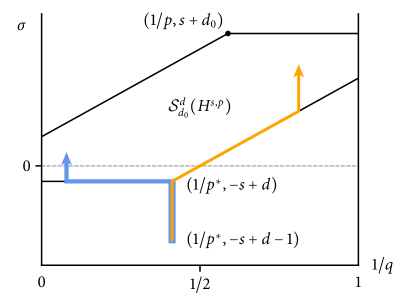
The specific sequence $(\sigma_{k},q_{k})$ can be achieved as follows, starting from $(\sigma_{1},q_{1})=(d-s,p^{*})$ , in two cases depending on whether $1/q\leq 1/p^{*}$ or not as depicted in Figure 3.

If $1/q\leq 1/p^{*}$ we first lower $1/q_{k}$ by steps of at most $1/n$ until it has been lowered to $1/q$ . At this point we raise $\sigma_{k}$ by steps of at most $1$ until it has been raised to $q$ . Note that at each step $k$ ,

\frac{1}{p}-\frac{s}{n}\leq\frac{1}{q}-\frac{\sigma}{n}\leq\frac{1}{q_{k}}-\frac{\sigma_{k}}{n}\leq\frac{1}{q_{1}}-\frac{\sigma_{1}}{n}=\frac{1}{p^{*}}-\frac{d-s}{n}

and hence the sequence remains in $\mathcal{S}^{d}_{0}(H^{s,p})$ as is required to apply Lemma 2.9. These same inequalities also show that conditions (H1:)–(H2:) are maintained at each step. Moreover, conditions (H3:)–(H4:) hold because we either fix $\sigma_{k}$ and lower $q_{k}$ by at most $1/n$ or we fix $q_{k}$ and raise $\sigma_{k}$ by at most $1$ .

Now suppose $1/q>1/p^{*}$ . Since $1/q-\sigma/n\leq 1/p^{*}-(d-s)/n$ , we can lower $\sigma$ to a value $\sigma^{\prime}$ such that the inequality becomes an equality. We now start the bootstrap by raising $\sigma_{k}$ to $\min(\sigma_{k}+1,\sigma^{\prime})$ at each step while simultaneously raising $1/q_{k}$ so that the value $1/q_{k}-\sigma_{k}/n=1/p^{*}-(d-s)/n$ remains invariant. This stage ends when $(\sigma_{k},q_{k})=(\sigma^{\prime},q)$ . We then increase $\sigma_{k}$ while leaving $q_{k}$ fixed as in the earlier argument when $1/q<1/p^{*}$ . The first stage of the sequence has $d-s\leq\sigma_{k}\leq\sigma^{\prime}\leq\sigma\leq s$ and

\frac{1}{p}-\frac{s}{n}\leq\frac{1}{q}-\frac{\sigma}{n}\leq\frac{1}{p^{*}}-\frac{d-s}{n}=\frac{1}{q_{k}}-\frac{\sigma_{k}}{n}.

Hence for this first part of the sequence the terms $(\sigma_{k},q_{k})$ lie in $\mathcal{S}^{d}_{0}(H^{s,p})$ and additionally conditions (H1:)–(H2:) are maintained. Moreover, condition (H3:) is enforced because we raise $\sigma_{k}$ by at most $1$ , and condition (H4:) is satisfied because it is an equality during this first stage where we lower $1/q_{k}$ . The same argument as in the case when $1/q\leq 1/p^{*}$ then shows that conditions (H1:)–(H4:) hold in the second stage when we raise $\sigma_{k}$ while leaving $q_{k}$ fixed. The proof is now complete in event that $d_{0}=0$ .

We now turn to the case $d_{0}>0$ where the bootstrap requires more care because the hypotheses of Lemma 2.9 are more restrictive. Consider the case $d_{0}=1$ . If $(\sigma,q)\in\mathcal{S}^{d}_{0}(H^{s,p})$ , we can simply apply the earlier result, so it suffices to assume $(\sigma,q)\in\mathcal{S}^{d}_{1}(H^{s,p}))$ but $(\sigma,q)\not\in\mathcal{S}^{d}_{0}(H^{s,p})$ . Because $d_{0}=1$ we can define a point $(\sigma^{\prime},q^{\prime})$ in $\mathcal{S}^{d}_{0}(H^{s,p})$ determined by $(\sigma,q)$ and the following rules:

1.

If $\sigma<s$ , leave $\sigma^{\prime}=\sigma$ fixed but raise $1/q$ by at most $1/n$ to $1/q^{\prime}$ such that $1/q^{\prime}-\sigma/n=1/p-s/n$ .
2.

If $\sigma\geq s$ and $1/p-s/n\leq 1/q-\sigma/n$ , lower $\sigma$ by at most 1 to $s$ while simultaneously lowering $1/q$ by at most $1/n$ so that the Lebesgue regularity $1/q-\sigma/n=1/q^{\prime}-\sigma^{\prime}/n$ is unchanged.
3.

Otherwise, $(\sigma,q)$ satisfies $s\leq\sigma\leq\sigma+1$ and

$\frac{1}{p}-\frac{s+1}{n}\leq\frac{1}{q}-\frac{\sigma}{n}<\frac{1}{p}-\frac{s}{n}$

and we set $(\sigma^{\prime},q^{\prime})=(s,p)$ .

In each of these cases $H^{s,q}(\Omega)$ is contained in $H^{s^{\prime},q^{\prime}}(\Omega)$ by Sobolev embedding, so we can apply the original bootstrap for $d_{0}=0$ to get to $(\sigma^{\prime},q^{\prime})$ . Since $(\sigma^{\prime},q^{\prime})\in\mathcal{S}^{d}_{0}(H^{s,p})$ a computation shows $(\sigma^{\prime}+1,q^{\prime})\in\mathcal{S}^{d_{0}}_{1}(H^{s,p})$ and hence the commutator result Lemma 2.9 can be applied at $(\sigma^{\prime},q^{\prime})$ . One verifies that in all three cases listed above, the target regularity $(\sigma,q)$ satisfies conditions (H1:)-(H4:) when starting from $(\sigma^{\prime},q^{\prime})$ and we can apply the bootstrap step exactly once to arrive at $(\sigma,q)$ . This proves the result when $d_{0}=1$ , and iterating this argument obtains the proof for any value of $d_{0}$ . ∎

3 Coefficients in Triebel-Lizorkin Spaces

This section generalizes the results of Section 2 to operators having coefficients in Triebel-Lizorkin spaces, which are defined defined in terms of Littlewood-Paley projection operators. Let $\phi$ be a smooth radial bump function that equals $1$ on $B_{1}$ and vanishes outside of $B_{2}$ and let $\psi(\xi)=\phi(\xi)-\phi(2\xi)$ , so $\psi(\xi)=0$ if $|\xi|>2$ or $|\xi|<1/2$ . For $k\in\mathbb{Z}$ we define the Littlewood-Paley projections $P_{k}$ and $P_{\leq k}$

	$\displaystyle\mathcal{F}[P_{k}u](\xi)$	$\displaystyle=\psi(2^{-k}\xi)\mathcal{F}[u](\xi)$
	$\displaystyle\mathcal{F}[P_{\leq k}u](\xi)$	$\displaystyle=\phi(2^{-k}\xi)\mathcal{F}[u](\xi).$

We also use the notation $P_{a\leq\cdot\leq b}$ for $\sum_{j=a}^{b}P_{j}$ .

Let $s\in\mathbb{R}$ and $1<p,q<\infty$ . Given a tempered distribution $u$ , each $P_{k}u$ is an analytic function on $\mathbb{R}^{n}$ and a tempered distribution belongs to the Triebel-Lizorkin space $F^{s,p}_{q}(\mathbb{R})$ if

||u||_{F^{s,p}_{q}(\mathbb{R}^{n})}=||P_{\leq 0}u||_{L^{p}(\mathbb{R}^{n})}+\left|\left|\,\,\left[\sum_{k=1}^{\infty}(2^{sk}|P_{k}u|)^{q}\,\,\right]^{1/q}\right|\right|_{L^{p}(\mathbb{R}^{n})}<\infty.

We call $p$ the Lebesgue parameter, whereas $q$ is the fine parameter. Bessel potential spaces are Triebel-Lizorkin spaces with fine parameter $q=2$ and, as recalled in the following section, Sobolev-Slobodeckij spaces $W^{s,p}(\mathbb{R}^{n})$ are also special cases of Triebel-Lizorkin spaces with either $q=2$ or $q=p$ . Just as for Bessel potential spaces, on an open set $\Omega\subseteq\mathbb{R}^{n}$ , $F^{s,p}_{q}(\Omega)$ consists of the restrictions to $\Omega$ of distributions in $F^{s,p}_{q}(\mathbb{R}^{n})$ to $\Omega$ and is given the quotient norm. The text [Tr10] contains a comprehensive description of Triebel-Lizorkin spaces, and indeed considers a wider set of parameters than those we employ here.

Embedding properties for Triebel-Lizorkin spaces follow those for Bessel potential spaces with the following rule of thumb: when a loss of derivatives is involved, the fine parameter has no role. Specifically, we recall the following results summarizing [Tr10] Proposition 2.3.2/2 and Theorems 2.7.1 and 3.3.1 along with [Tr78] Theorems 2.8.1 and 4.6.1; the notation $A\hookrightarrow B$ denotes a continuous inclusion of space $A$ into space $B$ . Note that here and elsewhere when we quote established results, we restrict the range of the parameters to $1<p,q<\infty$ even when they apply with greater generality.

Proposition 3.1.

Assume $1<p,p_{1},p_{2},q,q_{1},q_{2}<\infty$ and $s,s_{1},s_{2}\in\mathbb{R}$ , and suppose $\Omega$ is a bounded open set in $\mathbb{R}^{n}$ .

1.

If $s_{1}>s_{2}$ then $F^{s_{1},p}_{q_{1}}(\mathbb{R}^{n})\hookrightarrow F^{s_{2},p}_{q_{2}}(\mathbb{R}^{n})$ and $F^{s_{1},p}_{q_{1}}(\Omega)\hookrightarrow F^{s_{2},p}_{q_{2}}(\Omega)$ .
2.

If $q_{1}\leq q_{2}$ then $F^{s,p}_{q_{1}}(\mathbb{R}^{n})\hookrightarrow F^{s,p}_{q_{2}}(\mathbb{R}^{n})$ and $F^{s_{1},p}_{q_{1}}(\Omega)\hookrightarrow F^{s_{2},p}_{q_{2}}(\Omega)$ .
3.

If $p_{1}\geq p_{2}$ then $F^{s,p_{1}}_{q}(\Omega)\hookrightarrow F^{s,p_{2}}_{q}(\Omega)$ .
4.

If $s_{1}>s_{2}$ and $\frac{1}{p_{1}}-\frac{s_{1}}{n}=\frac{1}{p_{2}}-\frac{s_{2}}{n}$ then $F^{s_{1},p_{1}}_{q_{1}}(\mathbb{R}^{n})\hookrightarrow F^{s_{2},p_{2}}_{q_{2}}(\mathbb{R}^{n})$ .
5.

If $s_{1}>s_{2}$ and $\frac{1}{p_{1}}-\frac{s_{1}}{n}\leq\frac{1}{p_{2}}-\frac{s_{2}}{n}$ then $F^{s_{1},p_{1}}_{q_{1}}(\Omega)\hookrightarrow F^{s_{2},p_{2}}_{q_{2}}(\Omega)$ .
6.

If $0<\alpha<1$ then $F^{\frac{n}{p}+\alpha,p}_{q}(\mathbb{R}^{n})\hookrightarrow C^{0,\alpha}(\mathbb{R}^{n})$ and $F^{\frac{n}{p}+\alpha,p}_{q}(\Omega)\hookrightarrow C^{0,\alpha}(\Omega)$ .

Note that for bounded open sets $\Omega$ , [Tr10] and [Tr78] proves these embedding properties under the the addition hypothesis that $\Omega$ is a $C^{\infty}$ domain. The results for arbitrary bounded open sets follow as a corollary using the quotient space definition of the relevant spaces.

Complex interpolation of Triebel-Lizorkin spaces is described in [Tr10] Theorems 2.4.7 and 3.3.6.

Proposition 3.2.

Assume $1<p_{1},p_{2},q_{1},q_{2}<\infty$ and $s_{1},s_{2}\in\mathbb{R}$ , and suppose $\Omega$ is either $\mathbb{R}^{n}$ or is a bounded $C^{\infty}$ domain in $\mathbb{R}^{n}$ . For $0<\theta<1$ ,

[F^{s_{1},p_{1}}_{q_{1}}(\Omega),F^{s_{2},p_{2}}_{q_{2}}(\Omega)]_{\theta}=F^{s,p}_{q}(\Omega)

where

s=(1-\theta)s_{1}+\theta s_{2},\quad\frac{1}{p}=(1-\theta)\frac{1}{p_{1}}+\theta\frac{1}{p_{2}},\quad(1-\theta)\frac{1}{q_{1}}+\theta\frac{1}{q_{2}}.

Duality of spaces of functions on $\mathbb{R}^{n}$ follows from [Tr10] Theorem 2.11.2. Duality for Lipschitz bounded domains can be found in [Tr02], but the theory is more complex and we have avoided its use in our arguments; see, e.g., Proposition A.7.

Proposition 3.3.

Assume $1<p,q<\infty$ and $s\in\mathbb{R}$ . The bilinear map $\mathcal{D}(\mathbb{R}^{n})\times\mathcal{D}(\mathbb{R}^{n})\to\mathbb{R}$ given by $\left<f,g\right>:=\int_{\Omega}fg$ extends to a continuous bilinear map $F^{s,p}_{q}(\mathbb{R}^{n})\times F^{-s,p^{*}}_{q^{*}}(\mathbb{R}^{n})\to\mathbb{R}$ where $1/p^{*}=1-1/p$ and $1/q^{*}=1-1/q$ . Moreover, $f\mapsto\left<f,\cdot\right>$ is a continuous identification of $F^{s,p}_{q}(\mathbb{R}^{n})$ with $(F^{-s,p^{*}}_{q^{*}}(\mathbb{R}^{n}))^{*}$ .

3.1 Mapping properties

Operators with coefficients in Triebel-Lizorkin spaces are defined analogously to those of Definition 2.4.

Definition 3.4.

Suppose $d_{0},d\in\mathbb{Z}_{\geq 0}$ with $d_{0}\leq d$ . A differential operator on an open set $\Omega\subseteq\mathbb{R}^{n}$ of the form

\sum_{d_{0}\leq|\alpha|\leq d}a^{\alpha}\partial_{\alpha}

is of class $\mathcal{L}_{d_{0}}^{d}(F^{s,p}_{q};\Omega)$ for some $s\in\mathbb{R}$ , and $1<p,q<\infty$ if each

a^{\alpha}\in F^{s+|\alpha|-d,p}_{q}(\Omega).

We have the following multiplication rules for Triebel-Lizorkin spaces that generalize the rules found in Theorem 2.5. A self-contained proof is given in Appendix A.

Theorem 3.5.

Let $\Omega$ be a bounded open subset of $\mathbb{R}^{n}$ . Suppose $1<p_{1},p_{2},p,q_{1},q_{2},q<\infty$ and $s_{1},s_{2},s\in\mathbb{R}$ . Let $r_{1},r_{2}$ and $r$ be defined by

\frac{1}{r_{1}}=\frac{1}{p_{1}}-\frac{s_{1}}{n},\qquad\frac{1}{r_{2}}=\frac{1}{p_{2}}-\frac{s_{2}}{n},\quad\text{\rm and}\quad\frac{1}{r}=\frac{1}{p}-\frac{s}{n}.

Pointwise multiplication of $C^{\infty}(\overline{\Omega})$ functions extends to a continuous bilinear map $F^{s_{1},p_{1}}_{q_{1}}(\Omega)\times F^{s_{2},p_{2}}_{q_{2}}(\Omega)\rightarrow F^{s,p}_{q}(\Omega)$ so long as

$\displaystyle s_{1}+s_{2}$	$\displaystyle\geq 0$	(3.1)
$\displaystyle\min({s_{1},s_{2}})$	$\displaystyle\geq s$	(3.2)
$\displaystyle\max\left(\frac{1}{r_{1}},\frac{1}{r_{2}}\right)$	$\displaystyle\leq\frac{1}{r}$	(3.3)
$\displaystyle\frac{1}{r_{1}}+\frac{1}{r_{2}}$	$\displaystyle\leq 1$	(3.4)
$\displaystyle\frac{1}{r_{1}}+\frac{1}{r_{2}}$	$\displaystyle\leq\frac{1}{r}$	(3.5)

with the the following caveats:

•

Inequality (3.5) is strict if $\min(1/r_{1},1/r_{2},1-1/r)=0$ .
•

If $s_{i}=s$ for some $i$ then $1/q\leq 1/q_{i}$ .
•

If $s_{1}+s_{2}=0$ then $\frac{1}{q_{1}}+\frac{1}{q_{2}}\geq 1$ .
•

If $s_{1}=s_{2}=s=0$ then $\displaystyle\frac{1}{q}\leq\frac{1}{2}\leq\frac{1}{q_{i}}$ for $i=1,2$ .

Repeated applications of Theorem 3.5 lead to the following analogue of Proposition 2.6.

Proposition 3.6.

Let $\Omega$ be a bounded open set in $\mathbb{R}^{n}$ . Suppose $1<p,q,a,b<\infty$ , $s>n/p$ , $\sigma\in\mathbb{R}$ and $d,d_{0}\in\mathbb{Z}_{\geq 0}$ with $d\geq d_{0}$ . An operator of class $\mathcal{L}_{d_{0}}^{d}(F^{s,p}_{q};\Omega)$ extends from a map $C^{\infty}(\overline{\Omega})\mapsto\mathcal{D}^{\prime}(\Omega)$ to a continuous linear map $F^{\sigma,a}_{b}(\Omega)\mapsto F^{\sigma-d,a}_{b}(\Omega)$ so long as

	$\displaystyle\sigma$	$\displaystyle\in[d-s,s+d_{0}]$		(3.6)
	$\displaystyle\frac{1}{a}-\frac{\sigma}{n}$	$\displaystyle\in\left[\frac{1}{p}-\frac{s+d_{0}}{n},\frac{1}{p^{*}}-\frac{d-s}{n}\right]$		(3.6)

and so long as:

•

If $\sigma=s+d_{0}$ then $\frac{1}{q}\geq\frac{1}{b}$ .
•

If $\sigma=d-s$ then $\frac{1}{b}\geq\frac{1}{q^{*}}$ .

Moreover, operators in $\mathcal{L}_{d_{0}}^{d}(F^{s,p}_{q};\Omega)$ depend continuously on their coefficients $a^{\alpha}\in F^{s-d+\alpha,p}_{q}(\Omega)$ .

Note that in the Bessel potential case, $q=b=2$ in Proposition 3.6 and the supplemental conditions at $\sigma=s+d_{0}$ and $\sigma=d-s$ are always satisfied. We have the following generalization of Definition 2.7.

Definition 3.7.

Suppose $1<p,q<\infty$ , $s\in\mathbb{R}$ and $d,d_{0}\in\mathbb{Z}_{\geq 0}$ with $d\geq d_{0}$ . The compatible Sobolev indices for an operator of class $\mathcal{L}_{d_{0}}^{d}(F^{s,p}_{q};\Omega)$ is the set

\mathcal{S}_{d_{0}}^{d}(F^{s,p}_{q})\subseteq\mathbb{R}\times(1,\infty)\times(1,\infty)

of tuples $(\sigma,a,b)$ satisfying (3.6) along with the additional conditions at the end of Proposition 3.6 when $\sigma=s+d_{0}$ or $\sigma=d-s$ .

The proof of Lemma 2.8 generalizes to the Triebel-Lizorkin context with minimal changes, using Proposition 3.1 for facts about Sobolev embedding. The only interesting difference is that the marginal conditions at the end of Proposition 3.6 adds an additional condition when $s$ is the smallest possible value such that $\mathcal{S}_{d_{0}}^{d}(F^{s,p}_{q})$ is nonempty.

Lemma 3.8.

Suppose $1<p,q<\infty$ , $s\in\mathbb{R}$ and $d,d_{0}\in\mathbb{Z}_{\geq 0}$ with $d\geq d_{0}$ . Then $\mathcal{S}_{d_{0}}^{d}(F^{s,p}_{q})$ is nonempty if and only if

	$\displaystyle s$	$\displaystyle\geq(d-d_{0})/2\text{, and}$		(3.7)
	$\displaystyle\frac{1}{p}-\frac{s}{n}$	$\displaystyle\leq\frac{1}{2}-\frac{(d-d_{0})/2}{n}$		(3.8)

with the additional condition $q\leq 2$ in the marginal case $s=(d-d_{0})/2$ . If $S_{d_{0}}^{d}(F^{s,p}_{q})$ is non-empty then it contains $(s+d_{0},p,q)$ , $(d-s,p^{*},q^{*})$ , and $((d+d_{0})/2,2,2)$ . Moreover, if $(\sigma,a,b)\in\mathcal{S}_{d_{0}}^{d}(F^{s,p}_{q})$ , then we have the continuous inclusions of Fréchet spaces

F^{s+d_{0},p}_{q,\rm loc}(\mathbb{R}^{n})\subseteq F^{\sigma,a}_{b,\rm loc}(\mathbb{R}^{n})\subseteq F^{d-s,p^{*}}_{q^{*},\rm loc}(\mathbb{R}^{n}).

(3.9)

Just as in the Bessel potential case, if an operator of class $\mathcal{L}_{d_{0}}^{d}(F^{s,p}_{q};\Omega)$ is compatible with any indices at all, it acts on a compatible $L^{2}$ -based Bessel potential space, $F^{(d-d_{0})/2,2}_{2}(\Omega)=H^{(d-d_{0})/2,2}(\Omega)$ .

The following commutator result generalizes Lemma 2.9.

Lemma 3.9.

Suppose $1<p,q,a,b<\infty$ , $s>n/p$ , $\sigma\in\mathbb{R}$ and $d,d_{0}\in\mathbb{Z}_{\geq 0}$ with $d\geq d_{0}$ . Let $L$ be an operator of class $\mathcal{L}_{d_{0}}^{d}(F^{s,p}_{q};\Omega)$ and let $\phi\in\mathcal{D}(\Omega)$ . Then $[L,\phi]$ extends from a map $C^{\infty}(\overline{\Omega})\mapsto\mathcal{D}^{\prime}(\Omega)$ to a continuous linear map $F^{\sigma,a}_{b}(\Omega)\mapsto F^{\sigma-d+1,a}_{b}(\Omega)$ so long as $(\sigma+1,a,b)\in\mathcal{S}^{d}_{d_{0}}(F^{s,p}_{q})$ . Moreover, if $d_{0}=0$ , the same result holds if $(\sigma,a,b)\in\mathcal{S}^{d}_{0}(H^{s,p}_{q})$ .

Proof.

The proof in the case of general $d_{0}$ is a computation that follows the analogous part of the proof of Lemma 2.9. The only difference is that there are fine parameter restrictions that need to be checked. In the notation of Theorem 3.5, nontrivial restrictions could happen when $s_{i}=s$ , when $s_{1}+s_{2}=0$ and when $s_{1}=s_{2}=s=0$ . One readily verifies that under the given hypotheses that $s_{1}=s_{2}=s=0$ cannot happen and that in the remaining cases the fine parameter restrictions are always met.

If $d_{0}=0$ the proof again follows the strategy of Lemma 2.9. First we observe that $[L,\phi]=[\hat{L},\phi]$ where $\hat{L}$ is $L$ with its constant term eliminated. Using the case $d_{0}=1$ already proved we have continuity so long as $(\sigma+1,a,b)\in\mathcal{S}^{d}_{1}(F^{s,p}_{q})$ , and computation shows that if $(\sigma,a,b)\in\mathcal{S}^{d}_{0}(F^{s,p}_{q})$ then $(\sigma+1,a,b)\in\mathcal{S}^{d}_{1}(F^{s,p}_{q})$ . ∎

3.2 Rescaling estimates

In this section we show that the rescaling estimates of Proposition 2.10 carry over to Triebel-Lizorkin spaces.

Proposition 3.10.

Suppose $1<p,q<\infty$ , $s\in\mathbb{R}$ and that $\chi$ is a Schwartz function on $\mathbb{R}^{n}$ . There exists a constant $\alpha\in\mathbb{R}$ such that for all $0<r\leq 1$ and all $u\in F^{s,p}_{q}(\mathbb{R}^{n})$

||\chi u_{\{r\}}||_{F^{s,p}_{q}(\mathbb{R}^{n})}\lesssim r^{\alpha}||u||_{F^{s,p}_{q}(\mathbb{R}^{n})}.

(3.10)

Specifically:

1.

Inequality (3.10) holds with

$\alpha=\min\left(s-\frac{n}{p},0\right)$

unless $s-n/p=0$ , in which case it holds for any choice of $\alpha<0$ , with implicit constant depending on $\alpha$ .
2.

If $s>n/p$ (in which case functions in $F^{s,p}_{q}(\mathbb{R}^{n})$ are Hölder continuous) and if $u\in F^{s,p}_{q}(\mathbb{R}^{n})$ with $u(0)=0$ , then inequality holds with

$\alpha=\min\left(s-\frac{n}{p},1\right)$

unless $s-n/p=1$ , in which case it holds for any choice of $\alpha<1$ , with implicit constant depending on $\alpha$ .

The remainder of this section is an extended proof of this result, and relies on the following elementary facts from Littlewood-Paley theory.

Proposition 3.11.

Let $1<p,q,t<\infty$ .

1.

If $\eta$ is a Schwartz function then for any $M>0$ ,

$|(P_{k}\eta)(x)|\lesssim\frac{2^{-Mk}}{(1+|x|^{M})}$

with implicit constant independent of $x$ and $k$ but depending on $\eta$ and $M$ .

There exist Schwartz functions $\kappa,\kappa^{*}$ such that for any tempered distribution $u$ ,

	$\displaystyle(P_{k}u)(x)$	$\displaystyle=\int u(x+2^{-k}y)\kappa(y)\;dy$
	$\displaystyle(P_{\leq k}u)(x)$	$\displaystyle=\int u(x+2^{-k}y)\kappa^{*}(y)\;dy,$

with convolution and scaling interpreted in the distributional sense.

For all $u\in L^{p}(\mathbb{R}^{n})$ , $k\in\mathbb{N}$ , and $x\in\mathbb{R}^{n}$

	$\displaystyle\|P_{k}u(x)\|$	$\displaystyle\lesssim\|(Mu)(x)\|\quad\text{and}$
	$\displaystyle\|P_{\leq k}u(x)\|$	$\displaystyle\lesssim\|(Mu)(x)\|.$

Here $M$ is the Hardy-Littlewood maximal operator and the implicit constants are independent of $u$ , $k$ and $x$ .

For any sequence $\{f_{k}\}_{k\in\mathbb{N}}$ of functions in $L^{p}(\mathbb{R}^{n})$ ,

\left|\left|\,\,\left[\sum_{k\in\mathbb{N}}|P_{k}f_{k}|^{q}\right]^{1/q}\,\right|\right|_{L^{p}(\mathbb{R}^{n})}\lesssim\left|\left|\,\,\left[\,\,\sum_{k\in\mathbb{N}}|f_{k}|^{q}\right]^{1/q}\,\right|\right|_{L^{p}(\mathbb{R}^{n})}.

Let $s>0$ and $a\in\mathbb{N}$ . For all $u\in F^{s,p}_{q}(\mathbb{R}^{n})$ ,

||u||_{F^{s,p}_{q}(\mathbb{R}^{n})}\sim||u||_{L^{p}(\mathbb{R}^{n})}+\left|\left|\,\,\left[\sum_{k\geq a}|2^{sk}P_{k}u|^{q}\right]^{1/q}\,\right|\right|_{L^{p}(\mathbb{R}^{n})}.

6.
(Littlewood-Paley Trichotomy) Suppose $u\in L^{p}(\mathbb{R}^{n})$ and $v\in L^{t}(\mathbb{R}^{n})$ . Given $k,k^{\prime},k^{\prime\prime}\in\mathbb{Z}$ ,

$P_{k}((P_{k^{\prime}}u)(P_{k^{\prime\prime}}v))=0$

unless one of the following three conditions holds:
- •
  
  $k^{\prime}\leq k-4$ and $k-3\leq k^{\prime\prime}\leq k+3$ ,
- •
  
  $k-3\leq k^{\prime}\leq k+3$ and $k^{\prime\prime}\leq k+5$ ,
- •
  
  $k^{\prime}\geq k+4$ and $|k^{\prime}-k^{\prime\prime}|\leq 2$ .

Part (1) is a consequence of the definition of the projection operator and elementary properties of the Fourier transform. The proof of parts (2) and (3) can be found in the approachable lecture notes [Ta01], weeks 2/3. Part (4) in full generality follows from the Fefferman-Stein inequality [FS71] together with part (3). We note, however, that the cases of greatest interest (Bessel potential spaces and Sobolev-Slobodeckij spaces) only involve the cases $q=2$ and $q=p$ , which do not require the full power of [FS71]. The lecture notes [Ta01] contain a proof of part (4) when $q=2$ , and the result when $q=p$ is an easy consequence of part (3) and the Hardy-Littlewood maximal inequality. Part (5) follows from the definition of the norm, part (2) and embedding $F^{s,p}_{q}(\mathbb{R}^{n})\hookrightarrow F^{0,p}_{2}(\mathbb{R}^{n})=L^{p}(\mathbb{R}^{n})$ . Part (6) is just a computation based on the supports of convolutions of functions $\psi_{k}$ used to define Littlewood-Paley projection; see [Ta01] for a related statement. Note that there is an artificial asymmetry in part (6) between $k^{\prime}$ and $k^{\prime\prime}$ , and symmetry can be restored at the expense of increasing the number of cases.

As for Bessel potential spaces, rescaling $u\mapsto u_{\{r\}}$ is a continuous automorphism of any space $F^{s,p}_{q}(\mathbb{R}^{n})$ ; for $s>0$ this is a straightforward consequence of the Closed Graph Theorem, using the fact that rescaling is continuous acting on $L^{p}(\mathbb{R}^{n})$ , whereas for $s<0$ and $s=0$ the result follows from duality and interpolation respectively. We initially require the following basic estimate for the norms of the rescaling maps.

Lemma 3.12.

Let $R>0$ , and suppose $1<p,q<\infty$ and $s\in\mathbb{R}$ . Then

||u_{\{r\}}||_{F^{s,p}_{q}(\mathbb{R}^{n})}\lesssim||u||_{F^{s,p}_{q}(\mathbb{R}^{n})}

for all $u\in F^{s,p}_{q}(\mathbb{R}^{n})$ and all $r\in[-R,R]$ .

Proof.

Recall the cutoff functions $\phi$ and $\psi$ used to define the Littlewood-Paley projection operators and define

\psi_{k}(\xi)=\begin{cases}0&k<0\\ \phi(\xi)&k=0\\ \psi(2^{-k}\xi)&k>0\end{cases}

A computation shows that for $k\geq 0$ ,

(P_{k}u_{\{r\}})(x)=f_{k}(rx)

where $f_{k}=\mathcal{F}^{-1}M_{k}\mathcal{F}u$ and where

M_{k}(\xi)=\phi_{k}(r\xi).

From the bound $|r|\leq R$ we can find $J$ independent of $r$ such that

M_{k}=M_{k}\sum_{j=-J}^{J}\psi_{k+j}

with the convention that $\psi_{k}=0$ for $k<0$ . Hence

f_{k}=\sum_{j=-J}^{J}(\mathcal{F}^{-1}M_{k}\mathcal{F})[P_{k+j}u].

Using [Tr10] Theorem 1.6.3 via the same argument as in [Tr10] Proposition 2.3.2/1 we find

\int\left(\sum|f_{k}|^{q}\right)^{p/q}\lesssim\int\left(\sum|P_{k}u_{\{r\}}|^{q}\right)^{p/q}=||u||^{p}_{F^{s,p}_{q}(\mathbb{R}^{n})}

with implicit constant independent of $r\in[-R,R]$ . Recalling that $(P_{k}u_{\{r\}})(x)=f_{k}(rx)$ the result now follows from the obvious uniform bounds on rescaling in $L^{p}(\mathbb{R}^{n})$ for $|r|\leq R$ . ∎

We now proceed with the proof of Proposition 3.10 part (1) is broken into three cases depending on whether $s>0$ , $s<0$ , or $s=0$ . We begin with $s>0$ and first establish the following technical lemma, which is needed to control high frequency rescaling.

Lemma 3.13.

Suppose $s>0$ . For all $0<r\leq 1$ and all $u\in F^{s,p}_{q}(\mathbb{R}^{n})$ ,

\left|\left|\left[\sum_{k\geq 1}|2^{ks}P_{k}u_{\{r\}}|^{q}\right]^{1/q}\right|\right|_{L^{p}(\mathbb{R}^{n})}\lesssim r^{s-\frac{n}{p}}||u||_{F^{s,p}_{q}(\mathbb{R}^{n})}.

Proof.

Suppose first that $r=2^{-j}$ for some $j\in\mathbb{Z}_{\geq 0}$ . An easy computation from the definition of the Fourier transform and change of variables shows for each $k\in\mathbb{N}$ ,

(P_{k}u_{\{r\}})=(P_{k+j}u)_{\{r\}}

for all Schwartz functions $u$ , and hence also for all $u\in F^{s,p}_{q}(\mathbb{R}^{n})$ . But then

	$\displaystyle\left\|\left\|\left[\sum_{k\geq 1}\|2^{ks}P_{k}u_{\{r\}}\|^{q}\right]^{1/q}\right\|\right\|_{L^{p}(\mathbb{R}^{n})}$	$\displaystyle=2^{-js}\left\|\left\|\left[\sum_{k\geq 1+j}\|2^{ks}(P_{k}u)\|^{q}\right]^{1/q}\right\|\right\|_{L^{p}(\mathbb{R}^{n})}$
		$\displaystyle=2^{-js}2^{-n/p}\left\|\left\|\left[\sum_{k\geq 1+j}\|2^{ks}P_{k}u\|^{q}\right]^{1/q}\right\|\right\|_{L^{p}(\mathbb{R}^{n})}$
		$\displaystyle\lesssim 2^{-js}r^{-n/p}\|\|u\|\|_{F^{s,p}_{q}(\mathbb{R}^{n})}$
		$\displaystyle=r^{s-\frac{n}{p}}\|\|u\|\|_{F^{s,p}_{q}(\mathbb{R}^{n})}.$

This completes the proof in the case $r=2^{-j}$ . The general case follows from the consequence of Lemma 3.12 that that $u\mapsto u_{\{r\}}$ is uniformly bounded in $F^{s,p}_{q}(\mathbb{R}^{n})$ for $1/2\leq r\leq 2$ . ∎

Proposition 3.10 part (1) when $s>0$ now follows from the following.

Proposition 3.14.

Suppose $1<p,q<\infty$ and $s>0$ , and let $\chi$ be a Schwartz function. For all $u\in F^{s,p}_{q}(\mathbb{R}^{n})$ and $0<r\leq 1$ ,

||\chi u_{\{r\}}||_{F^{s,p}_{q}(\mathbb{R}^{n})}\lesssim r^{\alpha}||u||_{F^{s,p}_{q}(\mathbb{R}^{n})}

(3.11)

where

\alpha=\min\left(s-\frac{n}{p},0\right)

(3.12)

unless $s=n/p$ , in which case $\alpha$ can be any (fixed) negative number. The implicit constant in (3.11) depends on $\chi$ is independent of $u$ and $r$ .

Proof.

We first assume that $s\neq n/p$ and define $\alpha$ according to equation 3.12. Since $s>0$ , Proposition 3.11 part (5) implies

||\chi u_{\{r\}}||_{F^{s,p}_{q}(\mathbb{R}^{n})}\lesssim||\chi u_{\{r\}}||_{L^{p}(\mathbb{R}^{n})}+\left|\left|\left[\sum_{k\geq 10}|P_{k}(\chi u_{\{r\}})|^{q}\right]^{\frac{1}{q}}\right|\right|_{L^{p}(\mathbb{R}^{n})}.

(3.13)

To estimate the first term on the right-hand side of inequality (3.13) first consider the case $s<n/p$ . Define $t$ by

\frac{1}{t}=\frac{1}{p}-\frac{s}{n}

(3.14)

and observe that since $1/p<1$ and since $s<n/p$ , we have $0<1/t<1$ . Proposition 3.1 implies $F^{s,p}_{q}(\mathbb{R}^{n})$ embeds in $F^{0,t}_{2}(\mathbb{R}^{n})=L^{t}(\mathbb{R}^{n})$ . From Hölder’s inequality we find

||\chi u_{\{r\}}||_{L^{p}(\mathbb{R}^{n})}\leq||\chi||_{L^{\tau}(\mathbb{R}^{n})}||u_{\{r\}}||_{L^{t}(\mathbb{R}^{n})}

where $\frac{1}{\tau}=\frac{1}{p}-\frac{1}{t}$ . Hence, from Lemma 2.11

||u_{\{r\}}||_{L^{t}(\mathbb{R}^{n})}=r^{-\frac{n}{t}}||u||_{L^{t}(\mathbb{R}^{n})}=r^{s-\frac{n}{p}}||u||_{L^{t}(\mathbb{R}^{n})}\lesssim r^{\alpha}||u||_{F^{s,p}_{q}(\mathbb{R}^{n})}

and we conclude $||\chi u_{\{r\}}||_{L^{p}(\mathbb{R}^{n})}\lesssim r^{\alpha}||u||_{F^{s,p}_{q}(\mathbb{R}^{n})}$ . On the other hand, if $s>n/p$ then

||\chi u_{\{r\}}||_{L^{p}(\mathbb{R}^{n})}\lesssim||u_{\{r\}}||_{L^{\infty}(\mathbb{R}^{n})}||\chi||_{L^{p}(\mathbb{R}^{n})}\lesssim||u||_{F^{s,p}_{q}(\mathbb{R}^{n})}=r^{\alpha}||u||_{F^{s,p}_{q}(\mathbb{R}^{n})}.

Hence in both cases, $||\chi u_{\{r\}}||_{L^{p}(\mathbb{R}^{n})}\lesssim r^{\alpha}||u||_{F^{s,p}_{q}(\mathbb{R}^{n})}$ .

Turning to the second term on the right-hand side of inequality (3.13) we introduce the notation

\widetilde{P}_{k}=P_{k-3\leq\cdot\leq k+3}.

The Littlewood-Paley trichotomy, Proposition 3.11 part (6), implies

P_{k}(\chi u_{\{r\}})=P_{k}\left(\underbrace{(\widetilde{P}_{k}\chi)(P_{\leq k-4}u_{\{r\}})}_{\text{high-low}}+\underbrace{(P_{\leq k+5}\chi)\widetilde{P}_{k}u_{\{r\}})}_{\text{low-high}}+\underbrace{\sum_{k^{\prime}\geq k+4}(\widetilde{P}_{k^{\prime}}\chi)(P_{k^{\prime}}u_{\{r\}})}_{\text{high-high}}\right)

(3.15)

and we estimate the contributions from each of these three terms individually via the triangle inequality.

Starting with the high-low term, Proposition 3.11 parts (4) and (3) imply

	$\displaystyle\left\|\left\|\left[\sum_{k\geq 10}\|2^{sk}P_{k}\left\{\left(\widetilde{P}_{k}\chi\right)\left(P_{\leq k-4}u_{\{r\}}\right)\right\}\|^{q}\right]^{\frac{1}{q}}\right\|\right\|_{L^{p}(\mathbb{R}^{n})}$	$\displaystyle\lesssim\left\|\left\|\left[\sum_{k\geq 10}\|2^{sk}\left(\widetilde{P}_{k}\chi\right)\left(P_{\leq k-4}u_{\{r\}}\right)\|^{q}\right]^{\frac{1}{q}}\right\|\right\|_{L^{p}(\mathbb{R}^{n})}$
		$\displaystyle\lesssim\left\|\left\|\|Mu_{\{r\}}\|\left[\sum_{k\geq 10}\|2^{sk}\widetilde{P}_{k}\chi\|^{q}\right]^{\frac{1}{q}}\right\|\right\|_{L^{p}(\mathbb{R}^{n})}$

where $M$ is the Hardy-Littlewood maximal operator. Now suppose $s<n/p$ and pick $t$ according to equation (3.14). Then Hölder’s inequality and the triangle inequality imply

\left|\left||Mu_{\{r\}}|\left[\sum_{k\geq 10}|2^{sk}\widetilde{P}_{k}\chi|^{q}\right]^{\frac{1}{q}}\right|\right|_{L^{p}(\mathbb{R}^{n})}\lesssim||Mu_{\{r\}}||_{L^{t}(\mathbb{R}^{n})}||\chi||_{F^{s,\tau}_{q}(\mathbb{R}^{n})}

where again $1/\tau=1/p-1/t$ . The Hardy-Littlewood maximal inequality and Lemma 2.11 then imply $||Mu_{\{r\}}||_{L^{t}(\mathbb{R}^{n})}\lesssim||u_{\{r\}}||_{L^{t}(\mathbb{R}^{n})}\lesssim r^{-\frac{n}{t}}||u||_{L^{t}(\mathbb{R}^{n})}=r^{\alpha}||u||_{F^{s,p}_{q}(\mathbb{R}^{n})}$ , which yields the desired estimate

\left|\left|\left[\sum_{k\geq 10}|2^{ks}P_{k}\left\{\left(\widetilde{P}_{k}\chi\right)\left(P_{k-4}u_{\{r\}}\right)\right\}|^{q}\right]^{\frac{1}{q}}\right|\right|_{L^{p}(\mathbb{R}^{n})}\lesssim r^{\alpha}||u||_{F^{s,p}_{q}(\mathbb{R}^{n})}.

Obtaining this same inequality in the case $s>n/p$ is similar but easier, using the estimate

|Mu_{\{r\}}|\lesssim||u||_{L^{\infty}(\mathbb{R}^{n})}\lesssim||u||_{F^{s,p}_{q}(\mathbb{R}^{n})}=r^{\alpha}||u||_{F^{s,p}_{q}(\mathbb{R}^{n})}

along with the fact $\chi\in F^{s,p}_{q}(\mathbb{R}^{n})$ .

To estimate the low-high term we estimate $|P_{\leq k+5}\chi|\lesssim||\chi||_{L^{\infty}(\mathbb{R}^{n})}$ and use Proposition 3.11 part (4) and Lemma 3.13 to conclude

	$\displaystyle\left\|\left\|\left[\sum_{k\geq 10}\|P_{k}\left\{2^{ks}\left(P_{\leq k+5}\chi\right)\left(\widetilde{P}_{k}u_{\{r\}}\right)\right\}\|^{q}\right]^{\frac{1}{q}}\right\|\right\|_{L^{p}(\mathbb{R}^{n})}$	$\displaystyle\lesssim\left\|\left\|\left[\sum_{k\geq 10}\|2^{ks}\widetilde{P}_{k}u_{\{r\}}\|^{q}\right]^{\frac{1}{q}}\right\|\right\|_{L^{p}(\mathbb{R}^{n})}$
		$\displaystyle\lesssim\left\|\left\|\left[\sum_{k\geq 7}\|2^{ks}P_{k}u_{\{r\}}\|^{q}\right]^{\frac{1}{q}}\right\|\right\|_{L^{p}(\mathbb{R}^{n})}$
		$\displaystyle\lesssim r^{s-\frac{n}{p}}\|\|u\|\|_{F^{s,p}_{q}(\mathbb{R}^{n})}$
		$\displaystyle\lesssim r^{\alpha}\|\|u\|\|_{F^{s,p}_{q}(\mathbb{R}^{n})}.$

Finally, for the high-high term we observe from Proposition 3.11 part (2) that $\widetilde{P}_{j}\chi\lesssim 2^{-j}$ is uniformly bounded in $L^{\infty}(\mathbb{R}^{n})$ independent of $j$ and hence Proposition 3.11 part (4) and Lemma 3.13 along with the triangle inequality imply

	$\displaystyle\left\|\left\|\left[\sum_{k\geq 10}\left\|2^{ks}P_{k}\left\{\sum_{k^{\prime}\geq k+4}(P_{k^{\prime}}u_{\{r\}})(\widetilde{P}_{k^{\prime}}\chi)\right\}\right\|^{q}\right]^{\frac{1}{q}}\right\|\right\|_{L^{p}(\mathbb{R}^{n})}$	$\displaystyle\lesssim\left\|\left\|\left[\sum_{k\geq 10}\left\|2^{ks}\sum_{k^{\prime}\geq k+4}(P_{k^{\prime}}u_{\{r\}})(\widetilde{P}_{k^{\prime}}\chi)\right\|^{q}\right]^{\frac{1}{q}}\right\|\right\|_{L^{p}(\mathbb{R}^{n})}$
		$\displaystyle\lesssim\sum_{a\geq 4}2^{-as}\left\|\left\|\left[\sum_{k\geq 10}\left\|2^{(k+a)s}P_{k+a}u_{\{r\}}\right\|^{q}\right]^{\frac{1}{q}}\right\|\right\|_{L^{p}(\mathbb{R}^{n})}$
		$\displaystyle\lesssim\sum_{a\geq 4}2^{-as}\left\|\left\|\left[\sum_{k\geq 1}\|2^{ks}P_{k}u_{\{r\}}\|^{q}\right]^{\frac{1}{q}}\right\|\right\|_{L^{p}(\mathbb{R}^{n})}$
		$\displaystyle\lesssim r^{s-\frac{n}{p}}\|\|u\|\|_{F^{s,p}_{q}(\mathbb{R}^{n})}.$

This concludes the proof unless $s=n/p$ , in which case the result follows from interpolation. ∎

The proof of Proposition 3.10 part (1) when $s<0$ uses a duality argument analogous to that used for the same step in Section 2.2. First, the following generalization of Lemma 2.12 follows from [Tr10] Proposition 3.4.1/1, which is proved similarly to Lemma 3.13.

Lemma 3.15.

Suppose $1<p,q<\infty$ , and $s>0$ . For all $r\geq 1$ and all $u\in F^{s,p}_{q}(\mathbb{R}^{n})$ ,

||u_{\{r\}}||_{F^{s,p}_{q}(\mathbb{R}^{n})}\lesssim||u||_{F^{s,p}_{q}(\mathbb{R}^{n})}r^{s-\frac{n}{p}}.

(3.16)

The following corollary, which completes the case of part (1), is proved identically to Corollary 2.13 using the duality property of Proposition 3.3.

Corollary 3.16.

Suppose $1<p,q<\infty$ and $s<0$ . For all $0<r\leq 1$ and all $u\in F^{s,p}_{q}(\mathbb{R}^{n})$

||u_{\{r\}}||_{F^{s,p}_{q}(\mathbb{R}^{n})}\lesssim r^{\sigma-\frac{n}{p}}||u||_{F^{s,p}_{q}(\mathbb{R}^{n})}.

Proposition 3.10 part (1) has now been established except for the case $s=0$ , which follows from the following easy interpolation argument.

Lemma 3.17.

Suppose $1<p,q<\infty$ . For all $0<r\leq 1$ and all $u\in F^{0,p}_{q}(\mathbb{R}^{n})$ ,

||u_{\{r\}}||_{F^{0,p}_{q}(\mathbb{R}^{n})}\lesssim r^{-\frac{n}{p}}||u||_{F^{0,p}_{q}(\mathbb{R}^{n})}.

Proof.

Pick $\sigma\in\mathbb{R}$ such that $0<\sigma<n/p$ . Then for all Schwartz functions $u$ , Corollary 3.16 and Proposition 3.14 imply

	$\displaystyle\|\|u_{\{r\}}\|\|_{F^{\sigma,p}_{q}(\mathbb{R}^{n})}$	$\displaystyle\lesssim r^{\sigma-\frac{n}{p}}\|\|u\|\|_{F^{\sigma,p}_{q}(\mathbb{R}^{n})}$
	$\displaystyle\|\|u_{\{r\}}\|\|_{F^{-\sigma,p}_{q}(\mathbb{R}^{n})}$	$\displaystyle\lesssim r^{-\sigma-\frac{n}{p}}\|\|u\|\|_{F^{\sigma,p}_{q}(\mathbb{R}^{n})}.$

for all $0<r\leq 1$ . The result follows from interpolation. ∎

With the proof of Proposition 3.10 part (1) now complete we turn to part (2), the improved estimate when $u(0)=0$ . The following estimate is the key to controlling low-frequency interactions near $x=0$ .

Lemma 3.18.

Suppose $u\in C^{0,\alpha}(\mathbb{R}^{n})$ for some $\alpha\in(0,1]$ and that $u(0)=0$ . For all $k\in\mathbb{N}$ and all $0<r\leq 1$

|P_{\leq k}u_{\{r\}}(x)|\lesssim||u||_{C^{0,\alpha}(\mathbb{R}^{n})}\min(r^{\alpha}(|x|^{\alpha}+1),1).

Proof.

Proposition 3.11 part (2) implies there is a Schwartz function $\kappa^{*}$ such that

P_{\leq k}u_{\{r\}}(x)=\int u(rx+r2^{-k}y)\kappa^{*}(y)\;dy.

We therefore have the easy estimate $||P_{\leq k}u_{\{r\}}||_{L^{\infty}(\mathbb{R}^{n})}\lesssim||u||_{C^{0,\alpha}(\mathbb{R}^{n})}$ and it suffices to show

|P_{\leq k}u_{\{r\}}(x)|\lesssim||u||_{C^{0,\alpha}(\mathbb{R}^{n})}r^{\alpha}(|x|^{\alpha}+1)

as well.

Since $u(0)=0$ , on each annulus $A_{j}=\{y:2^{j}\leq|y|\leq 2^{j+1}\}$ for $j\in\mathbb{Z}_{\geq 0}$ we find

|u_{\{r\}}(x+2^{-k}y)|\leq||u||_{C^{0,\alpha}(\mathbb{R}^{n})}r^{\alpha}|x+2^{-k}y|^{\alpha}\lesssim r^{\alpha}||u||_{C^{0,\alpha}(\mathbb{R}^{n})}\left(|x|^{\alpha}+2^{\alpha j}\right)

where the implicit constant is independent of $j$ . Hence

\displaystyle\left|\int_{A_{j}}u(rx+r2^{-k}y)\kappa^{*}(y)\;dy\right|

\displaystyle\lesssim r^{\alpha}||u||_{C^{0,\alpha}(\mathbb{R}^{n})}\left(|x|^{\alpha}+2^{\alpha j}\right)\int_{A_{j}}|\kappa^{*}(y)|\;dy.

Since $\kappa^{*}$ is a Schwartz function, $\int_{A_{j}}|\kappa^{*}(y)|\;dy\lesssim 2^{-(1+\alpha)j}$ and hence

\left|\int_{A_{j}}u(rx+r2^{-k}y)\kappa^{*}(y)\;dy\right|\lesssim r^{\alpha}||u||_{C^{0,\alpha}(\mathbb{R}^{n})}(|x|^{\alpha}+1)2^{-j}.

(3.17)

On the other hand,

	$\displaystyle\left\|\int_{B_{1}(0)}u(rx+r2^{-k}y)\kappa^{*}(y)\;dy\right\|$	$\displaystyle\leq\|\|u\|\|_{C^{0,\alpha}(\mathbb{R}^{n})}r^{\alpha}(\|x\|+1)^{\alpha}\int_{B_{1}}\|\kappa^{*}(y)\|\;dy$		(3.18)
		$\displaystyle\lesssim\|\|u\|\|_{C^{0,\alpha}(\mathbb{R}^{n})}r^{\alpha}(\|x\|^{\alpha}+1).$		(3.18)

The result follows from adding the contributions in inequalities (3.17) and (3.18). ∎

Part (2) of Proposition 3.10 now follows from the following.

Proposition 3.19.

Suppose $1<p,q<\infty$ and $s>n/p$ , and let $\chi$ be a Schwartz function. For all $u\in F^{s,p}_{q}(\mathbb{R}^{n})$ with $u(0)=0$ , and for all $0<r\leq 1$ ,

||\chi u_{\{r\}}||_{F^{s,p}_{q}(\mathbb{R}^{n})}\lesssim r^{\alpha}||u||_{F^{s,p}_{q}(\mathbb{R}^{n})}

(3.19)

where

\alpha=\min\left(s-\frac{n}{p},1\right)

(3.20)

unless $s=n/p+1$ , in which case $\alpha$ can be any (fixed) number less than 1. The implicit constant in (3.19) depends on $\chi$ but is independent of $u$ and $r$ .

Proof.

We start by assuming $s\neq\frac{n}{p}+1$ and define $\alpha$ according to equation (3.20). Hence $F^{s,p}_{q}(\mathbb{R}^{n})$ embeds in $C^{0,\alpha}(\mathbb{R}^{n})$ .

As in the proof of Proposition 3.14 we start from the estimate

||\chi u_{\{r\}}||_{F^{s,p}_{q}(\mathbb{R}^{n})}\lesssim||\chi u_{\{r\}}||_{L^{p}(\mathbb{R}^{n})}+\left|\left|\left[\sum_{k\geq 10}\left|2^{ks}P_{k}(\chi u_{\{r\}})\right|^{q}\right]^{\frac{1}{q}}\right|\right|_{L^{p}(\mathbb{R}^{n})}.

(3.21)

The second term on the right-hand side is again estimated using the Littlewood-Paley trichotomy (equation (3.15)) and the proof of Proposition 3.14 shows that the low-high and high-high terms of that decomposition satisfy a bound of the form $r^{s-\frac{n}{p}}||u||_{F^{s,p}_{q}(\mathbb{R}^{n})}$ , regardless of the value of $u$ at zero. Consequently, we need only estimate the effects of the low-frequency contributions from $u_{\{r\}}$ , namely the high-low term, as well as $||\chi u_{\{r\}}||_{L^{p}(\mathbb{R}^{n})}$ .

For the low-high term, let $v_{r}(x)=\min(r^{\alpha}(|x|^{\alpha}+1),1)$ and hence Lemma 3.18 implies $|u_{\{r\}}|\lesssim||u||_{C^{0,\alpha}(\mathbb{R}^{n})}v_{r}$ for all $0<r\leq 1$ . Recalling the notation $\widetilde{P}_{k}=P_{k-3\leq\cdot\leq k+3}$ , Proposition 3.11 part 4 and Lemma 3.18 imply

	$\displaystyle\left\|\left\|\left[\sum_{k\geq 10}\left\|2^{ks}P_{k}\left\{\left(\widetilde{P}_{k}\chi\right)\left(P_{\leq k-4}u_{\{r\}}\right)\right\}\right\|^{q}\right]^{\frac{1}{q}}\right\|\right\|_{L^{p}(\mathbb{R}^{n})}$	$\displaystyle\lesssim\left\|\left\|\left[\sum_{k\geq 10}\left\|2^{ks}\left(\widetilde{P}_{k}\chi\right)\left(P_{\leq k-4}u_{\{r\}}\right)\right\|^{q}\right]^{\frac{1}{q}}\right\|\right\|_{L^{p}(\mathbb{R}^{n})}$		(3.22)
		$\displaystyle\lesssim\|\|u\|\|_{C^{0,\alpha}(\mathbb{R}^{n})}\|\|v_{r}\eta\|\|_{L^{p}(\mathbb{R}^{n})}$		(3.22)

where $\eta=\left[\sum_{k\geq 10}|2^{ks}\widetilde{P}_{k}\chi|^{q}\right]^{\frac{1}{q}}$ . Since $\chi$ is a Schwartz function, Proposition 3.11 part (1) implies that given $M>0$ we can estimate

|(P_{j}\chi)(x)|\lesssim\frac{2^{-Mj}}{(1+|x|)^{M}}

with implicit constant independent of $j$ . As a consequence, $|\eta(x)|\lesssim 1/(1+|x|)^{M}$ ; i.e., $\eta$ is rapidly decreasing.

To estimate $||v_{r}\eta||_{L^{p}(\mathbb{R}^{n})}$ we divide $\mathbb{R}^{n}$ into three regions: the ball $B_{1}(0)$ , the annulus $A=B_{1/r}(0)\setminus B_{1}(0)$ and the exterior region $E=B_{1/r}(0)^{c}$ . On the unit ball $|v_{r}|\lesssim r^{\alpha}$ and hence

||v_{r}\eta||_{L^{p}(B_{1}(0))}\lesssim r^{\alpha}.

(3.23)

Outside the unit ball, $|v_{r}(x)|\lesssim r^{\alpha}(|x|^{\alpha}+1)\lesssim r^{\alpha}|x|^{\alpha}$ and $|\eta(x)|\lesssim|x|^{-(n+1)/p-\alpha}$ So

\displaystyle\int_{A}\eta^{p}v_{r}^{p}

\displaystyle\lesssim\int_{1}^{1/r}s^{-n-1-\alpha p}(rs)^{\alpha p}s^{n-1}\;ds\leq r^{p\alpha}\int_{1}^{1/r}s^{-2}\;ds\lesssim r^{p\alpha}

(3.24)

Finally, for the exterior region we estimate $|v_{r}|\leq 2$ and find

\int_{E}\eta^{p}|v_{r}|^{p}\lesssim\int_{1/r}^{\infty}s^{-n-1-\alpha p}s^{n-1}\;ds\lesssim r^{1+\alpha p}\lesssim r^{\alpha p}.

(3.25)

Combining inequalities (3.23), (3.24) and (3.25) we conclude $||v_{r}\eta||_{L^{p}(\mathbb{R}^{n})}\lesssim r^{\alpha}$ which, when combined with inequality (3.22), completes the estimate for the low-high term.

It remains to show that $||\chi u_{\{r\}}||_{L^{p}(\mathbb{R}^{n})}\lesssim||u||_{F^{s,p}_{q}(\mathbb{R}^{n})}r^{\alpha}$ . The argument that showed $||v_{r}\eta||_{L^{p}(\mathbb{R}^{n})}\lesssim r^{\alpha}$ only used the fact that $\eta$ was rapidly decreasing, and hence we also find $||v_{r}\chi||_{L^{p}(\mathbb{R}^{n})}\lesssim r^{\alpha}$ . Again using the estimate $|u_{\{r\}}|\lesssim||u||_{C^{0,\alpha}(\mathbb{R}^{n})}v_{r}$ we obtain

||\chi u_{\{r\}}||_{L^{p}(\mathbb{R}^{n})}\lesssim||u||_{C^{0,\alpha}(\mathbb{R}^{n})}||\chi v_{r}||_{L^{p}(\mathbb{R}^{n})}\lesssim||u||_{F^{s,p}_{q}(\mathbb{R}^{n})}r^{\alpha}.

This concludes the proof assuming $s\neq\frac{n}{p}+1$ . For the marginal case, let $F^{s,p}_{q,0}(\mathbb{R}^{n})$ denote the closed subspace of $F^{s,p}_{q}(\mathbb{R}^{n}$ ) consisting of functions that vanish at zero, assuming of course that $s>n/p$ . The proof when $s=n/p+1$ follows from interpolation if we can show

[F^{s_{1},p}_{q,0}(\mathbb{R}^{n}),F^{s_{2},p}_{q,0}(\mathbb{R}^{n})]_{\theta}=F^{s,p}_{q,0}(\mathbb{R}^{n})

(3.26)

assuming that $s_{i}>n/p$ for $i=1,2$ and that $0<\theta<1$ and $s=s_{1}(1-\theta)+s_{2}\theta$ .

Let $\phi$ be a compactly supported smooth function with $\phi(0)=1$ . For smooth compactly supported functions $u$ define $Ru=u-u(0)\phi$ . This extends to a continuous retraction $F^{s,p}_{q}(\mathbb{R}^{n})\to F^{s,p}_{q,0}(\mathbb{R}^{n})$ so long as $s>n/p$ , with the co-retraction being the natural embedding. The interpolation property (3.26) now follows from, e.g, [Tr76] Lemma 6. ∎

3.3 Interior elliptic estimates

Elliptic operators for operators with coefficients in Triebel-Lizorkin spaces are defined analogously to Definition 2.18. This section contains our primary elliptic regularity result,

which relies on the following generalization of the rescaling estimates of Proposition 2.10. The proof of these estimates is a little involved, so we record the result for now and defer the proof to Section 3.2.

The “regularity at a point” result, Proposition 2.20, admits a straightforward generalization. Note that $\tilde{F}^{s,p}_{q}(\Omega)$ denotes the closure of $\mathcal{D}(\Omega)$ in $F^{s,p}_{q}(\mathbb{R}^{n})$ .

Proposition 3.20.

Let $\Omega\subset\mathbb{R}^{n}$ be a bounded open set. Suppose $1<p,q<\infty$ , $s\in\mathbb{R}$ , that $d,d_{0}\in\mathbb{Z}_{\geq 0}$ with $d_{0}\leq d$ , that $s>n/p$ , and that the conditions of Lemma 3.8 are are satisfied and hence $\mathcal{S}_{d_{0}}^{d}(F^{s,p}_{q})\neq\emptyset$ . Suppose additionally that $L=\sum_{|\alpha|\leq d}a^{\alpha}\partial_{\alpha}$ is a differential operator of class $\mathcal{L}_{d_{0}}^{d}(F^{s,p}_{q};\Omega)$ and that for some $x\in\Omega$ that

L_{0}=\sum_{|\alpha|=m}a^{\alpha}(x)\partial_{\alpha}

is elliptic. Given $(\sigma,a,b)\in\mathcal{S}_{d_{0}}^{d}(F^{s,p}_{q})$ there exists $r>0$ such that $B_{r}(x)\subset\Omega$ and such that if

	$\displaystyle u$	$\displaystyle\in\widetilde{F}^{d-s,p^{}}_{q^{}}(B_{r}(x))\quad\text{and}$
	$\displaystyle Lu$	$\displaystyle\in F^{\sigma-d,a}_{b}(\Omega)$

then $u\in F^{\sigma,a}_{b}(\Omega)$ and

||u||_{F^{\sigma,a}_{b}(\Omega)}\lesssim||Lu||_{F^{\sigma-d,a}_{b}(\Omega)}+||u||_{F^{d-s-1,p^{*}}_{q^{*}}(\Omega)}

(3.27)

with implicit constant independent of $u$ but depending on all other parameters.

Proof.

The proof is essentially the same as the proof of Proposition 2.20, with the following notes:

1.

The proof of the natural generalization of Lemma 2.19 regarding the parametrix goes through now using [Tr10] Theorems 2.3.7 and 2.3.8 in place of the Mikhlin multiplier theorem to establish the desired continuity properties.
2.

We replace the use of the rescaling result Proposition 2.17 with Proposition 3.10, which results in a little simplification because the replacement result is sharper.
3.

Fine parameters need tracking, but the changes are straightforward. When the Lebesgue parameter is $p$ the fine parameter is $q$ , when the Lebesgue parameter is $p^{*}$ the fine parameter is $q^{*}$ and for the intermediate spaces the Lebesgue parameter is $a$ and the fine parameter is $b$ .

∎

The proof of the main interior regularity result for Bessel potential spaces, Theorem 2.21, carries over to the Triebel-Lizorkin setting. The bulk of the new work consists of tracking the fine parameter.

Theorem 3.21.

Let $\Omega$ be a bounded open set in $\mathbb{R}^{n}$ and suppose $s,p,q,d_{0}$ and $d$ are parameters as in Lemma 3.8 such that $s>n/p$ and such that the conditions of Lemma 3.8 are satisfied so $\mathcal{S}_{d_{0}}^{d}(F^{s,p}_{q})\neq\emptyset$ . Suppose $L$ is of class $\mathcal{L}_{d_{0}}^{d}(F^{s,p}_{q};\Omega)$ and is elliptic on $\Omega$ . If $u\in F^{d-s,p^{*},q^{*}}(\Omega)$ and $Lu\in F^{\sigma-d,a}_{b}(\Omega)$ for some $(\sigma,a,b)\in\mathcal{S}_{d_{0}}^{d}(F^{s,a}_{b})$ then for any open set $U$ with $\overline{U}\subseteq\Omega$ , $u\in F^{\sigma,a}_{b}(U)$ and

||u||_{F^{\sigma,a}_{b}(U)}\lesssim||Lu||_{F^{\sigma-d,a}_{b}(\Omega)}+||u||_{F^{d-s-1,p^{*}}_{q^{*}}(\Omega)}.

(3.28)

Proof.

The proof follows that of Theorem 2.21 with the following changes needed to manage the fine parameter.

A bootstrap step starts with knowing $u\in F^{\sigma_{A},a_{A}}_{b_{A}}(\Omega_{A})$ for some open set $\Omega_{A}$ containing $\overline{U}$ and we wish to improve these parameters to $(\sigma_{B},a_{B},b_{B})$ while shrinking $\Omega_{A}$ . We assume:

H1:

$\sigma_{B}\leq\sigma$ ,
H2:

$\displaystyle\frac{1}{q}-\frac{\sigma}{n}\leq\frac{1}{q_{B}}-\frac{\sigma_{B}}{n}$ ,
H3:

$\sigma_{B}\leq\sigma_{A}+1$ ,
H4:

$\displaystyle\frac{1}{q_{A}}-\frac{\sigma_{A}+1}{n}\leq\frac{1}{q_{B}}-\frac{\sigma_{B}}{n}$ ,
H5:

if $\sigma_{B}=\sigma$ then $b_{B}\geq b$ ,
H6:

if $\sigma_{B}=\sigma_{A}+1$ then $b_{B}\geq b_{A}$ .

Hypotheses (H1:)–(H4:) are exactly those of Theorem (2.21) expressed in terms of the notation of the current result. Condition (H5:) is needed additionally to ensure $F^{\sigma,a}_{b}(\Omega)\subset F^{\sigma_{B},a_{B}}_{b_{B}}(\Omega)$ . Similarly (H6:) is the extra hypothesis needed to ensure $F^{\sigma_{A}+1,a_{A}}_{b_{A}}(\Omega_{A})\subset F^{\sigma_{B},a_{B}}_{b_{B}}(\Omega_{A})$ . If we additionally assume that $(\sigma_{A},a_{A},b_{A})$ satisfies the conditions of Lemma 3.9 so that its commutator estimate applies, the bootstrap step argument of Theorem 2.21 then goes through with obvious changes and we obtain an open set $\Omega_{B}$ with $\overline{U}\subset\Omega_{B}\subset\Omega_{A}$ such that $u\in F^{\sigma_{B},a_{B}}_{b_{B}}(\Omega_{B})$ along with the estimate

||u||_{F^{\sigma_{B},a_{B}}_{b_{B}}(\Omega_{B})}\lesssim||Lu||_{F^{\sigma-d,a}_{b}(\Omega)}+||u||_{F^{\sigma_{A},a_{A}}_{b_{A}}(\Omega_{A})}.

Now consider the bootstrap in the case $d_{0}=0$ where we pass through a sequence of regularity parameters $(\sigma_{k},a_{k},b_{k})$ starting from $(\sigma_{,}a_{0},b_{0})=(d-s-1,p^{*},q^{*})$ ; we need not track the shrinking open sets. Focusing for the moment only on the parameters $\sigma_{k}$ and $a_{k}$ , the bootstrap consists of three distinct stages:

1.

The initial step arriving at $(\sigma_{1},a_{1},b_{1})=(d-s,p^{*},q^{*})$ .
2.
A low regularity stage that either
- •
  
  preserves $\sigma_{k}=d-s$ while lowering $1/a_{k}$ by at most $1/n$ per step, or
- •
  
  preserves the Lebesgue regularity at the low value $1/p^{*}-(d-s)/n$ while raising $\sigma_{k}$ by at most 1 per step.
At the end of the low regularity stage $\sigma_{k}\leq\sigma$ and $a_{k}=a$ .
3.

A derivative improving stage where $a_{k}=a$ is fixed and $\sigma_{k}$ is raised by at most 1 per step until arriving at its final value.

We now discuss the sequence of fine parameters $b_{k}$ , which will in fact be set to $q^{*}$ throughout the sequence just described except at the last step, where it is set to its desired value.

1.

The initial stage starts at $(\sigma_{0},a_{0},b_{0})=(d-s-1,p^{*},q^{*})$ and wish to improve to $(-d+s,p^{*},q^{*})$ . Because $(\sigma_{0}+1,a_{0},b_{0})\in\mathcal{S}^{d}_{0}(F^{s,p}_{q})$ , the commutator result Lemma 3.9 applies. Hypotheses (H1:)–(H4:) hold for the same reasons as in Theorem 2.21. At this step, hypothesis (H5:) reads “if $d-s$ = $\sigma$ then $b\leq q^{*}$ ”, which is satisfied by the definition of $\mathcal{S}^{d}_{0}(F^{s,p}_{q})$ . Finally, hypothesis (H8:) holds trivially. Thus this first bootstrap step is justified.
2.
During the low regularity stage we again preserve $b_{k}=q^{*}$ at every step. This is justified as follows for the two possibilities:
- •
  
  Consider a step where $\sigma_{k}=d-s$ and where $1/a_{k}$ is lowered by at most $1/n$ . Conditions (H1:)–(H4:) are met for the same reasons as in Theorem (2.21) and condition (H8:) is met trivially. Condition (H7:) is a restriction only if $\sigma=d-s$ , in which case it requires $b\leq q^{*}$ ; this condition is met by the definition of $\mathcal{S}^{d}_{0}(F^{s,p}_{q})$ . We also need to ensure that the commutator estimate can be employed, which can be done by showing that $(\sigma_{k},a_{k},b_{k})=(d-s,a_{k},q^{*})\in\mathcal{S}^{d}_{0}(F^{s,p})$ . In fact, the definition of $\mathcal{S}^{d}_{0}(F^{s,p}_{q})$ permits the fine parameter to be $q^{*}$ along the line $\sigma=d-s$ , even in the marginal case $s=d-s$ where the region $S^{d}_{0}(F^{s,p}_{q})$ collapses to a line segment. The remainder of the justification of the commutator estimate is the same as in Theorem 2.21.
- •
  
  Consider a step where the Lebesgue regularity is preserved at the low value $1/p^{*}-(d-s)/n$ . and where $\sigma_{k}$ is raised by at most 1; without loss of generality we can assume we raise $\sigma_{k}$ by less than 1. Hypotheses (H1:)–(H4:) are met for the same reasons as in Theorem 2.21. Condition (H6:) is always met because of our additional restriction on the step size. Condition (H7:) only comes into play if we are raising $\sigma_{k}$ to its terminal value, in which case we also set the fine parameter to its terminal value $b$ (and stop the bootstrap). We need to ensure that each non-terminal $(\sigma_{k},a_{k},b_{k})$ lies in $S^{d}_{0}(F^{s,p}_{q})$ in order to apply the commutator estimate, but this is ensured because a fine parameter value of $q^{*}$ is always permitted along this line of Lebesgue regularity.
3.

On a step where we raise $\sigma_{k}$ and leave $a_{k}$ fixed at its terminal value we can again assume we raise $\sigma_{k}$ by less than 1. Throughout this stage we again leave $b_{k}$ fixed at $q^{*}$ except at the very last step. There are no fine parameter restrictions that arise to allow the commutator estimate to apply, and hypotheses (H1:)–(H4:) hold for the same reasons as in Theorem (2.21). Hypothesis (H6:) is always met because of our restriction on the step size and hypothesis (H7:) only comes into play at the final step, where we meet it by setting $b_{k}$ to its terminal value $b$ .

At this point of the procedure we have arrived at the desired parameters $(\sigma,a,b)$ , except in the marginal case $\sigma=d-s$ in which case we are at $(d-s,a,q^{*})$ . Since $\sigma=d-s$ , the definition of $\mathcal{S}^{d}_{0}(F^{s,p}_{q})$ implies $b\leq q^{*}$ and we can use this inequality to confirm that conditions (H1:)–(H8:) hold if we perform one more bootstrap step to improve the fine parameter to its desired value $b$ ; note that the commutator result Lemma (3.9) is available for this bootstrap step since $(d-s,a,q^{*})\in\mathcal{S}^{d}_{0}(F^{s,p}_{q})$ .

Now consider the case where $d_{0}=1$ . As in Theorem 2.21 it suffices to consider assume $(\sigma,a,b)\in\mathcal{S}^{d}_{1}(F^{s,p}_{q})$ but $(\sigma,a,b)\not\in\mathcal{S}^{d}_{0}(F^{s,p}_{q})$ . Starting from $(\sigma,a,b)$ we define $(\sigma^{\prime},a^{\prime},b^{\prime})\in\mathcal{S}^{d}_{0}(F^{s,p}_{q})$ by setting $b^{\prime}=\max(q,b)$ and then applying the following rules:

1.

If $\sigma<s$ , leave $\sigma^{\prime}=\sigma$ fixed but raise $1/a$ by at most $1/n$ to $1/a^{\prime}$ such that $1/a^{\prime}-\sigma/n=1/p-s/n$ .
2.

If $\sigma\geq s$ and $1/p-s/n\leq 1/a-\sigma/n$ , lower $\sigma$ by at most 1 to $s$ while simultaneously lowering $1/a$ by at most $1/n$ so that the Lebesgue regularity $1/a-\sigma/n=1/a^{\prime}-\sigma^{\prime}/n$ is unchanged.
3.

Otherwise, $(\sigma,a)$ satisfies $s\leq\sigma\leq\sigma+1$ and

$\frac{1}{p}-\frac{s+1}{n}\leq\frac{1}{a}-\frac{\sigma}{n}<\frac{1}{p}-\frac{s}{n}$

and we set $(\sigma^{\prime},a^{\prime})=(s,p)$ .

Note that we set $b^{\prime}=\max(q,b)$ to satisfy the fine parameter restriction on $\mathcal{S}^{d}_{0}(F^{s,p}_{q})$ when $\sigma^{\prime}=s$ . In all of these three cases, $F^{\sigma,a}_{b}(\Omega)$ is contained in $F^{\sigma^{\prime},a^{\prime}}_{b^{\prime}}(\Omega)$ and we can therefore apply the $d_{0}=0$ bootstrap to arrive at $(\sigma^{\prime},a^{\prime},b^{\prime})$ . Since $(\sigma^{\prime},a^{\prime},b^{\prime})\in\mathcal{S}_{0}^{d}(F^{s,p}_{q})$ , a computation shows that $(\sigma^{\prime}+1,a^{\prime},b^{\prime})\in\mathcal{S}_{1}^{d}(F^{s,p}_{q})$ and hence the commutator result from Lemma 3.9 can be applied starting from $(\sigma^{\prime},a^{\prime},b^{\prime})$ . Hence we can apply one round of the bootstrap starting from $(\sigma_{A},a_{A},b_{A})=(\sigma^{\prime},a^{\prime},b^{\prime})$ to arrive at $(\sigma_{B},a_{B},b_{B})=(\sigma,a,b)$ so long as hypotheses (H1:)–(H6:) are met. The first four are satisfied for the same reasons as in Theorem 2.21 and (H5:) is satisfied trivially since $b_{B}=b$ . Finally, (H6:) is a restriction only if $\sigma_{B}=\sigma_{A}+1$ , in which case $\sigma=s+1$ . But then, since $(\sigma,a,b)\in\mathcal{S}^{d}_{1}(F^{s,p}_{q})$ , we have assumed $q\leq b$ and hence $b^{\prime}=\max(q,b)=b$ . So we are not changing the fine parameter and condition (H6:) is met. This completes the proof when $d_{0}=1$ , and the result for higher values of $d_{0}$ follows from iterating this argument. ∎

4 Coefficients in Sobolev-Slobodeckij Spaces

Sobolev-Slobodeckij spaces of functions on an open set $\Omega\subset\mathbb{R}^{n}$ are special cases of Triebel-Lizorkin spaces as follows:

W^{s,p}(\Omega)=\begin{cases}F^{s,p}_{2}(\Omega)&s\in\mathbb{Z}\\ F^{s,p}_{p}(\Omega)&s\not\in\mathbb{Z}.\end{cases}

Hence the results of Section 3 specialize to statements about Sobolev-Slobodeckij spaces, which we briefly record here.

Definition 4.1.

Suppose $d_{0},d\in\mathbb{Z}_{\geq 0}$ with $d_{0}\leq d$ . A differential operator on an open set $\Omega\subseteq\mathbb{R}^{n}$ of the form

\sum_{d_{0}\leq|\alpha|\leq d}a^{\alpha}\partial_{\alpha}

is of class $\mathcal{L}_{d_{0}}^{d}(W^{s,p};\Omega)$ for some $s\in\mathbb{R}$ and $1<p<\infty$ if each

a^{\alpha}\in W^{s+|\alpha|-d,p}(\Omega).

Theorem 4.2.

Suppose $1<p_{1},p_{2},p<\infty$ and $s_{1},s_{2},s\in\mathbb{R}$ . Let $r_{1},r_{2}$ and $r$ be defined by

\frac{1}{r_{1}}=\frac{1}{p_{1}}-\frac{s_{1}}{n},\qquad\frac{1}{r_{2}}=\frac{1}{p_{2}}-\frac{s_{2}}{n},\quad\text{\rm and}\quad\frac{1}{r}=\frac{1}{p}-\frac{s}{n}.

Pointwise multiplication of $C^{\infty}(\overline{\Omega})$ functions extends to a continuous bilinear map $W^{s_{1},p_{1}}(\Omega)\times W^{s_{2},p_{2}}(\Omega)\rightarrow W^{s,p}(\Omega)$ so long as

$\displaystyle s_{1}+s_{2}$	$\displaystyle\geq 0$	(4.1)
$\displaystyle\min({s_{1},s_{2}})\geq\sigma$		(4.2)
$\displaystyle\max\left(\frac{1}{r_{1}},\frac{1}{r_{2}}\right)$	$\displaystyle\leq\frac{1}{r}$	(4.3)
$\displaystyle\frac{1}{r_{1}}+\frac{1}{r_{2}}$	$\displaystyle\leq 1$	(4.4)
$\displaystyle\frac{1}{r_{1}}+\frac{1}{r_{2}}$	$\displaystyle\leq\frac{1}{r}$	(4.5)

with the the following caveats:

•

Inequality (4.5) is strict if $\min(1/r_{1},1/r_{2},1-1/r)=0$ .
•

If $s=s_{i}\not\in\mathbb{Z}$ , then $p=p_{i}$ , $i=1,2$ .
•

If $s_{1},s_{2}\not\in\mathbb{Z}$ and $s_{1}+s_{2}=0$ then $\frac{1}{p_{1}}+\frac{1}{p_{2}}=1$ .

Proposition 4.3.

Let $\Omega$ be a bounded open subset of $\mathbb{R}^{n}$ . Suppose $1<p,q<\infty$ , $s>n/p$ , $\sigma\in\mathbb{R}$ and $d,d_{0}\in\mathbb{Z}_{\geq 0}$ with $d\geq d_{0}$ . An operator of class $\mathcal{L}_{d_{0}}^{d}(W^{s,p};\Omega)$ extends from a map $C^{\infty}(\overline{\Omega})\mapsto\mathcal{D}^{\prime}(\Omega)$ to a continuous linear map $W^{\sigma,q}(\Omega)\mapsto W^{\sigma-d,q}(\Omega)$ so long as

	$\displaystyle\sigma$	$\displaystyle\in[d-s,s+d_{0}]$		(4.6)
	$\displaystyle\frac{1}{q}-\frac{\sigma}{n}$	$\displaystyle\in\left[\frac{1}{p}-\frac{s+d_{0}}{n},\frac{1}{p^{*}}-\frac{d-s}{n}\right]$		(4.6)

and so long as:

•

If $s\not\in\mathbb{Z}$ and $\sigma=s+d_{0}$ then $q=p$ .
•

If $s\not\in\mathbb{Z}$ and $\sigma=d-s$ then $q=p^{*}$ .

Moreover, operators in $\mathcal{L}_{d_{0}}^{d}(W^{s,p};\Omega)$ depend continuously on their coefficients $a^{\alpha}\in W^{s,p+|\alpha|-d}(\Omega)$ .

Definition 4.4.

\mathcal{S}_{d_{0}}^{d}(W^{s,p})\subseteq\mathbb{R}\times(1,\infty)

of tuples $(\sigma,q)$ satisfying (4.6) along with the additional conditions at the end of Proposition 4.3 when $\sigma=s+d_{0}$ or $\sigma=d-s$ .

Lemma 4.5.

Suppose $1<p<\infty$ , $s\in\mathbb{R}$ and $d,d_{0}\in\mathbb{Z}_{\geq 0}$ with $d\geq d_{0}$ . Then $\mathcal{S}_{d_{0}}^{d}(W^{s,p})$ is nonempty if and only if

	$\displaystyle s$	$\displaystyle\geq(d-d_{0})/2\text{, and}$		(4.7)
	$\displaystyle\frac{1}{p}-\frac{s}{n}$	$\displaystyle\leq\frac{1}{2}-\frac{(d-d_{0})/2}{n}$		(4.8)

with the additional condition when $s\not\in\mathbb{Z}$ that $p=2$ in the marginal case $s=(d-d_{0})/2$ . If $S_{d_{0}}^{d}(W^{s,p})$ is non-empty then it contains $(s+d_{0},p)$ , $(d-s,p^{*})$ , and $((d+d_{0})/2,2)$ . Moreover, if $(\sigma,q)\in\mathcal{S}_{d_{0}}^{d}(W^{s,p})$ , then we have the continuous inclusions of Fréchet spaces

W^{s+d_{0},p}_{\rm loc}(\mathbb{R}^{n})\subseteq W^{\sigma,q}_{\rm loc}(\mathbb{R}^{n})\subseteq W^{d-s,p^{*}}_{\rm loc}(\mathbb{R}^{n}).

(4.9)

Theorem 4.6.

Let $\Omega$ be a bounded open set in $\mathbb{R}^{n}$ and suppose $s,p,d_{0}$ and $d$ are parameters as in Lemma 4.5 such that $s>n/p$ and such that the conditions of Lemma 4.5 are satisfied so $\mathcal{S}_{d_{0}}^{d}(W^{s,p})\neq\emptyset$ . Suppose $L$ is of class $\mathcal{L}_{d_{0}}^{d}(W^{s,p};\Omega)$ and is elliptic on $\Omega$ . If $u\in W^{d-s,p^{*}}(\Omega)$ and $Lu\in W^{\sigma-d,q}(\Omega)$ for some $(\sigma,q)\in\mathcal{S}_{d_{0}}^{d}(W^{s,p})$ then for any open set $U$ with $\overline{U}\subseteq\Omega$ , $u\in W^{\sigma,q}(U)$ and

||u||_{W^{\sigma,q}(U)}\lesssim||Lu||_{W^{\sigma-d,q}(\Omega)}+||u||_{W^{d-s-1,p^{*}}(\Omega)}.

(4.10)

5 Coefficients in Besov Spaces

We establish results for operators with coefficients in Besov spaces, mirroring the developments of the preceding sections. Recall from Section 3 the Littlewood-Paley projectors $P_{k}$ and $P_{\leq k}$ . Let $1<p,q<\infty$ and $s\in\mathbb{R}$ . A tempered distribution $u$ belongs to the Besov space $B^{s,p}_{q}(\mathbb{R}^{n})$ if

||u||_{B^{s,p}_{q}(\mathbb{R}^{n})}=\left\|P_{\leq 0}u\right\|_{L^{p}(\mathbb{R}^{n})}+\left(\sum_{k\geq 1}2^{sqk}\|P_{k}u\|_{L^{p}(\mathbb{R}^{n})}^{q}\right)^{\frac{1}{q}}<\infty.

(5.1)

On an open set $\Omega\subseteq\mathbb{R}^{n}$ , the space $B^{s,p}_{q}(\Omega)$ consists of the restrictions of distributions in $B^{s,p}_{q}(\mathbb{R}^{n})$ to $\Omega$ and is given the quotient norm.

Embedding properties of Besov spaces can be found in [Tr10] Proposition 2.3.2/2, and Theorems 2.7.1 and 3.3.1 along with [Tr78] Theorems 2.8.1 and 4.6.1; we summarize these in the following proposition. The important distinction here from Triebel-Lizorkin spaces is that when performing Sobolev embedding, the fine parameter cannot be improved if the Lebesgue regularity $1/p-s/n$ stays fixed. This phenomenon is the source of many of the additional fine parameter restrictions in this section beyond those of Section 3.

Proposition 5.1.

Assume $1<p,p_{1},p_{2},q,q_{1},q_{2}<\infty$ and $s,s_{1},s_{2}\in\mathbb{R}$ , and suppose $\Omega$ is a bounded open set in $\mathbb{R}^{n}$ .

1.

If $s_{1}>s_{2}$ then $B^{s_{1},p}_{q_{1}}(\mathbb{R}^{n})\hookrightarrow B^{s_{2},p}_{q_{2}}(\mathbb{R}^{n})$ and $B^{s_{1},p}_{q_{1}}(\Omega)\hookrightarrow B^{s_{2},p}_{q_{2}}(\Omega)$ .
2.

If $q_{1}\leq q_{2}$ then $B^{s,p}_{q_{1}}(\mathbb{R}^{n})\hookrightarrow B^{s,p}_{q_{2}}(\mathbb{R}^{n})$ and $B^{s,p}_{q_{1}}(\Omega)\hookrightarrow B^{s,p}_{q_{2}}(\Omega)$ .
3.

If $p_{1}\geq p_{2}$ then $B^{s,p_{1}}_{q}(\Omega)\hookrightarrow B^{s,p_{2}}_{q}(\Omega)$ .
4.

If $s_{1}>s_{2}$ and $\frac{1}{p_{1}}-\frac{s_{1}}{n}=\frac{1}{p_{2}}-\frac{s_{2}}{n}$ then $B^{s_{1},p_{1}}_{q}(\mathbb{R}^{n})\hookrightarrow B^{s_{2},p_{2}}_{q}(\mathbb{R}^{n})$ and $B^{s_{1},p_{1}}_{q}(\Omega)\hookrightarrow B^{s_{2},p_{2}}_{q}(\Omega)$ .
5.

If $s_{1}>s_{2}$ and $\frac{1}{p_{1}}-\frac{s_{1}}{n}<\frac{1}{p_{2}}-\frac{s_{2}}{n}$ then $B^{s_{1},p_{1}}_{q_{1}}(\Omega)\hookrightarrow B^{s_{2},p_{2}}_{q_{2}}(\Omega)$ .
6.

If $0<\alpha<1$ then $B^{\frac{n}{p}+\alpha,p}_{q}(\mathbb{R}^{n})\hookrightarrow C^{0,\alpha}(\mathbb{R}^{n})$ and $B^{\frac{n}{p}+\alpha,p}_{q}(\Omega)\hookrightarrow C^{0,\alpha}(\Omega)$ .

As noted previously following Proposition 3.1, although [Tr10] and [Tr78] only prove the embedding results above for bounded domains when the boundary is smooth, the result for arbitrary bounded open sets is an easy corollary.

Complex interpolation of Besov spaces ([Tr10] Theorems 2.4.7 and 3.3.6) follows the same pattern as for Triebel-Lizorkin spaces.

Proposition 5.2.

Assume $1<p_{1},p_{2},q_{1},q_{2}<\infty$ and $s_{1},s_{2}\in\mathbb{R}$ , and suppose $\Omega$ is either $\mathbb{R}^{n}$ or is a bounded $C^{\infty}$ domain in $\mathbb{R}^{n}$ . For $0<\theta<1$ ,

[B^{s_{1},p_{1}}_{q_{1}}(\Omega),B^{s_{2},p_{2}}_{q_{2}}(\Omega)]_{\theta}=B^{s,p}_{q}(\Omega)

where

s=(1-\theta)s_{1}+\theta s_{2},\quad\frac{1}{p}=(1-\theta)\frac{1}{p_{1}}+\theta\frac{1}{p_{2}},\quad(1-\theta)\frac{1}{q_{1}}+\theta\frac{1}{q_{2}}.

Duality for Besov spaces of functions on $\mathbb{R}^{n}$ is analogous to that for Triebel-Lizorkin spaces; see [Tr10] Theorem 2.11.2.

Proposition 5.3.

Assume $1<p,q<\infty$ and $s\in\mathbb{R}$ . The bilinear map $\mathcal{D}(\mathbb{R}^{n})\times\mathcal{D}(\mathbb{R}^{n})\to\mathbb{R}$ given by $\left<f,g\right>:=\int_{\Omega}fg$ extends to a continuous bilinear map $B^{s,p}_{q}(\mathbb{R}^{n})\times B^{-s,p^{*}}_{q^{*}}(\mathbb{R}^{n})\to\mathbb{R}$ . Moreover, $f\mapsto\left<f,\cdot\right>$ is a continuous identification of $B^{s,p}_{q}(\mathbb{R}^{n})$ with $(B^{-s,p^{*}}_{q^{*}}(\mathbb{R}^{n}))^{*}$ .

5.1 Mapping properties

As for the other function spaces, mapping properties of differential operators depend on the rules for multiplication in Besov spaces. We recall the relevant result here, and give a self-contained proof in Appendix B.

Theorem 5.4.

Let $\Omega$ be a bounded open subset of $\mathbb{R}^{n}$ . Suppose $1<p_{1},p_{2},p,q_{1},q_{2},q<\infty$ and $s_{1},s_{2},s\in\mathbb{R}$ . Let $r_{1},r_{2}$ and $r$ be defined by

\frac{1}{r_{1}}=\frac{1}{p_{1}}-\frac{s_{1}}{n},\qquad\frac{1}{r_{2}}=\frac{1}{p_{2}}-\frac{s_{2}}{n},\quad\text{\rm and}\quad\frac{1}{r}=\frac{1}{p}-\frac{s}{n}.

Pointwise multiplication of $C^{\infty}(\overline{\Omega})$ functions extends to a continuous bilinear map $B^{s_{1},p_{1}}_{q_{1}}(\Omega)\times B^{s_{2},p_{2}}_{q_{2}}(\Omega)\to B^{s,p}_{q}(\Omega)$ so long as

$\displaystyle\min(s_{1},s_{2})$	$\displaystyle\geq s$	(5.2)
$\displaystyle s_{1}+s_{2}$	$\displaystyle\geq 0$	(5.3)
$\displaystyle\max\left(\frac{1}{r_{1}},\frac{1}{r_{2}}\right)$	$\displaystyle\leq\frac{1}{r}$	(5.4)
$\displaystyle\frac{1}{r_{1}}+\frac{1}{r_{2}}$	$\displaystyle\leq 1$	(5.5)
$\displaystyle\frac{1}{r_{1}}+\frac{1}{r_{2}}$	$\displaystyle\leq\frac{1}{r}$	(5.6)

with the following caveats:

•

If $s=s_{i}$ or $1/r=1/r_{i}$ for some $i$ then $1/q\leq 1/q_{i}$ .
•

If $s_{1}+s_{2}=0$ or $1/r_{1}+1/r_{2}=1$ then $1/q_{1}+1/q_{2}\geq 1$ .
•
If equality holds in (5.6) then
- $\circ$
  
  $\min(1/r_{1},1/r_{2},1-1/r)\neq 0$ .
- $\circ$
  
  If $\min(s_{1},s_{2})\leq 0$ then $1/q_{1}+1/q_{2}\geq 1$ and $1/q\leq 1/r$ .
- $\circ$
  
  If $s_{i}$ has the same sign as $\min(s_{1},s_{2})$ for some $i$ then $1/q\leq 1/q_{i}$ .
- $\circ$
  
  If $s_{i}$ has the same sign as $\max(s_{1},s_{2})$ for some $i$ then $1/r_{i}\leq 1/q_{i}$ .
- $\circ$
  
  If $s=0$ then $1/q\leq 1/q_{i}$ and $1/r_{i}\leq 1/q_{i}$ for both $i=1,2$ .
•

If $s_{1}=s_{2}=s=0$ then $\displaystyle\frac{1}{q}\leq\min\left(\frac{1}{2},\frac{1}{r}\right)$ and $\displaystyle\max\left(\frac{1}{2},\frac{1}{r_{i}}\right)\leq\frac{1}{q_{i}}$ for both $i=1,2$ .

The list of caveats above is extensive in comparison with Theorem 3.5, but the bulk of these occur when inequality (5.6) is not strict, and we do not encounter this edge case in our applications.

Operators with coefficients in Besov spaces are defined analogously to those of Definition 2.4.

Definition 5.5.

Suppose $d_{0},d\in\mathbb{Z}_{\geq 0}$ with $d_{0}\leq d$ . A differential operator on an open set $\Omega\subseteq\mathbb{R}^{n}$ of the form

\sum_{d_{0}\leq|\alpha|\leq d}a^{\alpha}\partial_{\alpha}

is of class $\mathcal{L}_{d_{0}}^{d}(B^{s,p}_{q};\Omega)$ for some $s\in\mathbb{R}$ and $1<p,q<\infty$ if each

a^{\alpha}\in B^{s+|\alpha|-d,p}_{q}(\Omega).

Theorem 5.4 implies the following. Notably, in the computations that lead to this result, the caveats of Theorem 5.4 concerning the edge cases $1/r_{1}+1/r_{2}=1/r$ and $s_{1}=s_{2}=s=0$ never occur.

Proposition 5.6.

Let $\Omega$ be a bounded open subset of $\mathbb{R}^{n}$ . Suppose $1<p,q,a,b<\infty$ , $s>n/p$ , $\sigma\in\mathbb{R}$ and $d,d_{0}\in\mathbb{Z}_{\geq 0}$ with $d\geq d_{0}$ . An operator of class $\mathcal{L}_{d_{0}}^{d}(B^{s,p}_{q};\Omega)$ extends from a map $C^{\infty}(\overline{\Omega})\mapsto\mathcal{D}^{\prime}(\Omega)$ to a continuous linear map $B^{\sigma,a}_{b}(\Omega)\mapsto B^{\sigma-d,a}_{b}(\Omega)$ so long as

	$\displaystyle\sigma$	$\displaystyle\in[d-s,s+d_{0}]$		(5.7)
	$\displaystyle\frac{1}{a}-\frac{\sigma}{n}$	$\displaystyle\in\left[\frac{1}{p}-\frac{s+d_{0}}{n},\frac{1}{p^{*}}-\frac{d-s}{n}\right]$		(5.7)

and so long as:

•

If $\sigma=s+d_{0}$ or $\frac{1}{a}-\frac{\sigma}{n}=\frac{1}{p}-\frac{s+d_{0}}{n}$ then $\frac{1}{b}\leq\frac{1}{q}$ .
•

If $\sigma=d-s$ or $\frac{1}{a}-\frac{\sigma}{n}=\frac{1}{p^{*}}-\frac{d-s}{n}$ then $\frac{1}{b}\geq\frac{1}{q^{*}}$ .

Moreover, operators in $\mathcal{L}_{d_{0}}^{d}(B^{s,p}_{q};\Omega)$ depend continuously on their coefficients $a^{\alpha}\in B^{s-d+|\alpha|,p}_{q}(\Omega)$ .

We have the following generalization of Definition 2.7.

Definition 5.7.

Suppose $1<p,q<\infty)$ , $s\in\mathbb{R}$ and $d,d_{0}\in\mathbb{Z}_{\geq 0}$ with $d\geq d_{0}$ . The compatible Sobolev indices for an operator of class $\mathcal{L}_{d_{0}}^{d}(B^{s,p}_{q};\Omega)$ is the set

\mathcal{S}_{d_{0}}^{d}(B^{s,p}_{q})\subseteq\mathbb{R}\times(1,\infty)\times(1,\infty)

of tuples $(\sigma,a,b)$ satisfying (5.7) along with the additional conditions at the end of Proposition 5.6 in any of the boundary cases $\sigma=s+d_{0}$ , $\sigma=d-s$ , $1/a-\sigma/n=1/p-s/n$ or $1/a-\sigma/n=1/p^{*}-(d-s)/n$ .

The analogue of Lemma 2.8 in the Besov context is the following.

Lemma 5.8.

Suppose $1<p,q<\infty$ , $s\in\mathbb{R}$ and $d,d_{0}\in\mathbb{Z}_{\geq 0}$ with $d\geq d_{0}$ . Then $\mathcal{S}_{d_{0}}^{d}(B^{s,p}_{q})$ is nonempty if and only if

	$\displaystyle s$	$\displaystyle\geq(d-d_{0})/2\text{, and}$		(5.8)
	$\displaystyle\frac{1}{p}-\frac{s}{n}$	$\displaystyle\leq\frac{1}{2}-\frac{(d-d_{0})/2}{n}$		(5.9)

with the additional condition $q\leq 2$ in each of the marginal cases $s=(d-d_{0})/2$ and $\frac{1}{p}-\frac{s}{n}=\frac{1}{2}-\frac{(d-d_{0})/2}{n}$ . If $S_{d_{0}}^{d}(B^{s,p}_{q})$ is non-empty then it contains $(s+d_{0},p,q)$ , $(d-s,p^{*},q^{*})$ , and $((d+d_{0})/2,2,2)$ . Moreover, if $(\sigma,a,b)\in\mathcal{S}_{d_{0}}^{d}(B^{s,p}_{q})$ , then we have the continuous inclusions of Fréchet spaces

B^{s+d_{0},p}_{q,\rm{loc}}(\mathbb{R}^{n})\subseteq B^{\sigma,a}_{b,\rm{loc}}(\mathbb{R}^{n})\subseteq B^{d-s,p^{*}}_{q^{*},\rm{loc}}(\mathbb{R}^{n}).

(5.10)

The following commutator result is the analogue of Lemma 3.9

Lemma 5.9.

Suppose $1<p,q,a,b<\infty$ , $s>n/p$ , $\sigma\in\mathbb{R}$ and $d,d_{0}\in\mathbb{Z}_{\geq 0}$ with $d\geq d_{0}$ . Let $\Omega$ be a bounded open subset of $\mathbb{R}^{n}$ and let $L$ be an operator of class $\mathcal{L}_{d_{0}}^{d}(B^{s,p}_{q};\Omega)$ . If $\phi\in\mathcal{D}(\Omega)$ then $[L,\phi]$ extends from a map $C^{\infty}(\overline{\Omega})\mapsto\mathcal{D}^{\prime}(\Omega)$ to a continuous linear map $B^{\sigma,a}_{b}(\Omega)\mapsto B^{\sigma-d+1,a}_{b}(\Omega)$ so long as $(\sigma+1,a,b)\in\mathcal{S}^{d}_{d_{0}}(B^{s,p}_{q})$ . Moreover, if $d_{0}=0$ , the same result holds if $(\sigma,a,b)\in\mathcal{S}^{d}_{0}(B^{s,p}_{q})$ .

Proof.

The proof is a computation using Theorem 5.4 that parallels that of Lemma 3.9. The only difference is that there are three additional fine parameter restrictions that arise. In the notation of Theorem 5.4, these occur when $r=r_{i}$ , when $1/r_{1}+1/r_{2}=1$ and when $1/r_{1}+1/r_{2}=1/r$ . Under the given hypotheses, the last of these conditions never occurs, and in remaining two cases the fine parameter restrictions are met for the same reasons as the analogous restrictions are met when $s=s_{i}$ and when $s_{1}+s_{2}=0$ in Lemma 3.9. ∎

5.2 Rescaling estimates

The same argument used for Triebel-Lizorkin spaces shows that rescaling $u\mapsto u_{\{r\}}$ is a continuous automorphism of Besov spaces, and we wish to generalize the associated estimates of Theorem 3.10 to the Besov setting. This could be accomplished by suitably modifying the arguments of Section 3.2, but we can prove the desired results as a corollary of the Triebel-Lizorkin estimates using the following real interpolation property, which follows from [Tr10] Theorem 2.4.2.

Proposition 5.10.

Assume $1<p,q_{1},q_{2},q<\infty$ and $s_{1},s_{2}\in\mathbb{R}$ with $s_{1}\neq s_{2}$ . Suppose $0<\theta<1$ and let $s=(1-\theta)s_{1}+\theta s_{2}$ . Then

[F^{s_{1},p}_{q_{1}}(\mathbb{R}^{n}),F^{s_{2},p}_{q_{2}}(\mathbb{R}^{n})]_{\theta,q}=B^{s,p}_{q}(\mathbb{R}^{n}).

Proposition 5.11.

||\chi u_{\{r\}}||_{B^{s,p}_{q}(\mathbb{R}^{n})}\lesssim r^{\alpha}||u||_{B^{s,p}_{q}(\mathbb{R}^{n})}.

(5.11)

Specifically:

1.

Inequality (5.11) holds with

$\alpha=\min\left(s-\frac{n}{p},0\right)$

unless $s-n/p=0$ , in which case it holds for any choice of $\alpha<0$ , with implicit constant depending on $\alpha$ .
2.

If $s>n/p$ (in which case functions in $B^{s,p}_{q}(\mathbb{R}^{n})$ are Hölder continuous) and if $u\in B^{s,p}_{q}(\mathbb{R}^{n})$ with $u(0)=0$ , then inequality holds with

$\alpha=\min\left(s-\frac{n}{p},1\right)$

unless $s-n/p=1$ , in which case it holds for any choice of $\alpha<1$ , with implicit constant depending on $\alpha$ .

Proof.

Suppose $s<n/p$ . Pick $\epsilon>0$ such that $s_{1}=s+\epsilon<n/p$ as well, and let $s_{2}=s-\epsilon$ . From real interpolation with endpoints $F^{s_{1},p}_{2}(\mathbb{R}^{n})$ and $F^{s_{2},p}_{2}(\mathbb{R}^{n})$ along with Proposition 3.10 we find

||u_{r}||_{B^{s,p}_{q}(\mathbb{R}^{n})}\lesssim r^{\frac{1}{2}\left(s_{1}-\frac{n}{p}\right)+\frac{1}{2}\left(s_{2}-\frac{n}{p}\right)}||u||_{B^{s,p}_{q}(\mathbb{R}^{n})}=r^{s-\frac{n}{p}}||u||_{B^{s,p}_{q}(\mathbb{R}^{n})}.

A similar and easier proof works when $s>n/p$ and the marginal case $s=n/p$ can be handled by interpolation between endpoints with differentiability $s_{1}$ and $s_{2}$ taken arbitrarily close to $s$ , as in the proof of Proposition 2.17.

For the improved estimate in the Hölder continuous case, we let $F^{s,p}_{q,0}(\mathbb{R}^{n})$ be the closed subspace of $F^{s,p}_{q}(\mathbb{R}^{n})$ of functions that vanish at $0$ , assuming of course that $s>n/p$ . The spaces $B^{s,p}_{q,0}$ are defined similarly. The same argument as at the end of the proof of Proposition 3.19 shows that

[F^{s_{1},p}_{q_{1},0}(\mathbb{R}^{n}),F^{s_{2},p}_{q_{2},0}(\mathbb{R}^{n})]_{\theta,q}=B^{s,p}_{q,0}(\mathbb{R}^{n})

(5.12)

assuming that $s_{i}>n/p$ for $i=1,2$ and that $0<\theta<1$ and $s=(1-\theta)s_{1}+\theta s_{2}$ . Using this interpolation property, the proof of the improved estimate now follows exactly as in the generic case. ∎

5.3 Interior elliptic estimates

Elliptic operators with Besov space coefficients are defined analogously as in Definition 2.18. The following “regularity at a point” result is proved identically as for Proposition 3.20, using the fact that the parametrix result Lemma 2.19 is proved identically for Besov spaces. Note that $\widetilde{B}^{s,p}_{q}(\Omega)$ denotes the closure of $\mathcal{D}(\Omega)$ in $B^{s,p}_{q}(\mathbb{R}^{n})$ .

Proposition 5.12.

Let $\Omega\subset\mathbb{R}^{n}$ be a bounded open set. Suppose $s\in\mathbb{R}$ , $1<p,q<\infty$ , that $d,d_{0}\in\mathbb{Z}_{\geq 0}$ with $d_{0}\leq d$ , that $s>n/p$ , and that the conditions of Lemma 5.8 are are satisfied and hence $\mathcal{S}_{d_{0}}^{d}(B^{s,p}_{q})\neq\emptyset$ . Suppose additionally that $L=\sum_{|\alpha|\leq d}a^{\alpha}\partial_{\alpha}$ is a differential operator of class $\mathcal{L}_{d_{0}}^{d}(B^{s,p}_{q};\Omega)$ and that for some $x\in\Omega$ that

L_{0}=\sum_{|\alpha|=m}a^{\alpha}(x)\partial_{\alpha}

is elliptic. Given $(\sigma,a,b)\in\mathcal{S}_{d_{0}}^{d}(F^{s,p}_{q})$ there exists $r>0$ such that $B_{r}(x)\subset\Omega$ and such that if

	$\displaystyle u$	$\displaystyle\in\widetilde{B}^{d-s,p^{}}_{q^{}}(B_{r}(x))\quad\text{and}$
	$\displaystyle Lu$	$\displaystyle\in B^{\sigma-d,a}_{b}(\Omega)$

then $u\in B^{\sigma,a}_{b}(\Omega)$ and

||u||_{B^{\sigma,a}_{b}(\Omega)}\lesssim||Lu||_{B^{\sigma-d,a}_{b}(\Omega)}+||u||_{B^{d-s-1,p^{*}}_{q^{*}}(\Omega)}

(5.13)

with implicit constant independent of $u$ but depending on all other parameters.

With the previous proposition established, local elliptic regularity is proved using the same techniques as in Theorem 3.21, taking into account extra fine-parameter restrictions that arise for Besov spaces.

Theorem 5.13.

Let $\Omega$ be a bounded open set in $\mathbb{R}^{n}$ and suppose $s,p,d_{0}$ and $d$ are parameters as in Lemma 5.8 such that $s>n/p$ and such that the conditions of Lemma 5.8 are satisfied so $\mathcal{S}_{d_{0}}^{d}(B^{s,p}_{q})\neq\emptyset$ . Suppose $L$ is of class $\mathcal{L}_{d_{0}}^{d}(B^{s,p}_{q};\Omega)$ and is elliptic on $\Omega$ . If $u\in B^{d-s,p^{*}}_{q^{*}}(\Omega)$ and $Lu\in B^{\sigma-d,a}_{b}(\Omega)$ for some $(\sigma,a,b)\in\mathcal{S}_{d_{0}}^{d}(B^{s,p}_{q})$ then for any open set $U$ with $\overline{U}\subseteq\Omega$ , $u\in B^{\sigma,a}_{b}(U)$ and

||u||_{B^{\sigma,a}_{b}(U)}\lesssim||Lu||_{B^{\sigma-d,a}_{b}(\Omega)}+||u||_{B^{d-s-1,p^{*}}_{q^{*}}(\Omega)}.

(5.14)

Proof.

The proof very closely follows that of Theorem 3.21, and we list here the additional steps needed to further manage the fine parameter.

In addition to conditions (H1:)–(H6:) from that proof, the bootstrap step requires two more hypotheses to ensure the needed embeddings:

H7:

if $\frac{1}{a_{B}}-\frac{\sigma_{B}}{n}=\frac{1}{a}-\frac{\sigma}{n}$ then $b_{B}\geq b$ ,
H8:

if $\frac{1}{a_{B}}-\frac{\sigma_{B}}{n}=\frac{1}{a_{A}}-\frac{\sigma_{A}+1}{n}$ then $b_{B}\geq b_{A}$ .

For the stages of the main bootstrap for $d_{0}=0$ from Theorem 3.21 we make the following adjustments

1.

In the initial step from $(\sigma_{0},a_{0},b_{0})=(d-s-1,p^{*},q^{*})$ to $(\sigma_{1},a_{1},b_{1})=(d-s,p^{*},q^{*})$ hypothesis (H8:) is met trivially and hypothesis (H7:) only yields a restriction if $\frac{1}{p^{*}}-\frac{d-s}{n}=\frac{1}{a}-\frac{\sigma}{n}$ , in which case it requires $b\leq q^{*}$ . But this fine parameter restriction is met because $(\sigma,a,b)=(d-s,a,b)\in\mathcal{S}^{d}_{0}(B^{s,p}_{q})$ .
2.
During the low regularity stage we again preserve $b_{k}=q^{*}$ .
- •
  
  If we preserve $\sigma_{k}=d-s$ and lower $1/a_{k}$ we can arrange to do so by less than $1/n$ . In this case hypothesis (H8:) is met automatically. Hypothesis (H7:) only applies if $\sigma=d-s$ and only on the last step where we lower $1/a_{k}$ , in which case we set the fine parameter to its final value (satisfying (H7:)) and the bootstrap stops. All other aspects of this stage are justified identically to Theorem 3.21.
- •
  
  If we preserve the Lebesgue regularity $1/p^{*}-(d-s)/n$ and raise $\sigma_{k}$ then hypothesis (H8:) is met automatically. Hypothesis (H7:) provides a restriction only if $1/a-\sigma/n=1/p^{*}-(d-s)/n$ , in which case we have assumed $b\leq q^{*}$ from the definition of $\mathcal{S}^{d}_{0}(B^{s,p}_{q})$ and condition (H7:) is met. We need to ensure that the iterates $(\sigma_{k},a_{k},b_{k})$ all remain in $S^{d}_{0}(B^{s,p}_{q})$ in order for the commutator result Lemma 5.9 to apply. Indeed, the line of Lebesgue regularity $1/p^{*}-(d-s)/n$ is associated with a fine parameter restriction, but it is always met by keeping $b_{k}=q^{*}$ .
3.

In the final stage we raise $\sigma_{k}$ (by less than 1 per iteration) while keeping $a_{k}=a$ . Again we preserve $b_{k}=q^{*}$ except at the final step. Hypothesis (H8:) is met because of the step size restriction and hypothesis (H7:) is a restriction only at the last step, at which point it is satisfied by setting the fine parameter to its terminal value $b$ .

At the end of this procedure, the bootstrap has stopped at its desired value except in the two marginal cases $\sigma=d-s$ and $1/a-\sigma/n=1/p^{*}-(d-s)/n$ , in which case we have arrived at $(\sigma,a,q^{*})$ . In both these cases the definition of $\mathcal{S}^{d}_{0}(B^{s,p}_{q})$ ensures that $b<q^{*}$ . Using this inequality, one readily verifies that hypotheses (H1:)–(H8:) hold if we perform one more bootstrap step to improve the fine parameter to its final value $b$ . As in the proof of Theorem 3.21, one needs to verify that the starting regularity $(\sigma,a,q^{*})$ for the bootstrap lies in $\mathcal{S}^{d}_{0}(B^{s,p}_{q})$ so as to use the commutator result Lemma 5.9, but this is always met for the fine parameter $q^{*}$ on the two marginal lines $\sigma=d-s$ and $1/a-\sigma/n=1/p^{*}-(d-s)/n$ . This completes the proof when $d_{0}=0$ .

Now consider the case $d_{0}=1$ . Arguing as in Theorem 3.21, we can apply the $d_{0}=0$ bootstrap to arrive at some $(\sigma^{\prime},a^{\prime},b^{\prime})\in\mathcal{S}^{d}_{0}(B^{s,p}_{q})$ where $b^{\prime}=\max(q,b)$ and where $(\sigma^{\prime},a^{\prime})$ is obtained from $(\sigma,a)$ as follows:

1.

If $\sigma<s$ , leave $\sigma^{\prime}=\sigma$ fixed but raise $1/a$ by at most $1/n$ to $1/a^{\prime}$ such that $1/a^{\prime}-\sigma/n=1/p-s/n$ .
2.

If $\sigma\geq s$ and $1/p-s/n\leq 1/a-\sigma/n$ , lower $\sigma$ by at most 1 to $s$ while simultaneously lowering $1/a$ by at most $1/n$ so that the Lebesgue regularity $1/a-\sigma/n=1/a^{\prime}-\sigma^{\prime}/n$ is unchanged.
3.

Otherwise, $(\sigma,a)$ satisfies $s\leq\sigma\leq\sigma+1$ and

$\frac{1}{p}-\frac{s+1}{n}\leq\frac{1}{a}-\frac{\sigma}{n}<\frac{1}{p}-\frac{s}{n}$

and we set $(\sigma^{\prime},a^{\prime})=(s,p)$ .

Note that we set $b^{\prime}=\max(q,b)$ to ensure that the fine parameter restrictions of $\mathcal{S}^{d}_{0}(B^{s,p}_{q})$ along the lines $\sigma^{\prime}=s$ and $1/a^{\prime}-\sigma^{\prime}/n=1/p-s/n$ are met. Since $B^{\sigma,a}_{b}(\Omega)$ embeds in $B^{\sigma^{\prime},a^{\prime}}_{b^{\prime}}(\Omega)$ we can initially apply the $d_{0}=0$ bootstrap to arrive at $(\sigma^{\prime},a^{\prime},b^{\prime})$ . At this point we wish to apply a single bootstrap step to terminate at $(\sigma,a,b)$ . Since $(\sigma^{\prime},a^{\prime},b^{\prime})\in\mathcal{S}^{d}_{0}(B^{s,p}_{q})$ a computation shows $(\sigma^{\prime}+1,a^{\prime},b^{\prime})\in\mathcal{S}^{d}_{1}(B^{s,p}_{q})$ and hence the commutator Lemma 5.9 is available starting from $(\sigma^{\prime},a^{\prime},b^{\prime})$ . Hence we can perform the desired bootstrap step if we show that hypotheses (H1:)–(H8:) hold with $(\sigma_{A},a_{A},b_{A})=(\sigma^{\prime},a^{\prime},b^{\prime})$ and $(\sigma_{B},a_{B},b_{B})=(\sigma,a,b)$ .

Conditions (H1:)–(H4:) hold for the same reasons as in Theorem 2.21 and conditions (H5:) and (H7:) hold trivially since we are setting the fine parameter to $b$ . Condition (H6:) holds for exactly the same reason as in Theorem 3.21. Finally, condition (H8:) implies a restriction only in cases (1) and (3) and only when $1/a-\sigma/n=1/p-(s+1)/n$ . But then $(\sigma,a,b)\in\mathcal{S}^{d}_{1}(B^{s,p}_{q})$ is a spot where the fine parameter restriction $q\leq b$ holds and hence $b^{\prime}=\max(q,b)=b$ already. Hence condition (H8:) is met.

This concludes the proof when $d_{0}=1$ and the result holds for higher values of $d_{0}$ by iterating this argument. ∎

Appendix A Multiplication in Triebel-Lizorkin Spaces

We prove the multiplication rules for Triebel-Lizorkin spaces, Theorem 3.5, which we restate here for convenience.

Theorem 3.5.

Let $\Omega$ be a bounded open subset of $\mathbb{R}^{n}$ . Suppose $1<p_{1},p_{2},p,q_{1},q_{2},q<\infty$ and $s_{1},s_{2},s\in\mathbb{R}$ . Let $r_{1},r_{2}$ and $r$ be defined by

\frac{1}{r_{1}}=\frac{1}{p_{1}}-\frac{s_{1}}{n},\qquad\frac{1}{r_{2}}=\frac{1}{p_{2}}-\frac{s_{2}}{n},\quad\text{\rm and}\quad\frac{1}{r}=\frac{1}{p}-\frac{s}{n}.

Pointwise multiplication of $C^{\infty}(\Omega)$ functions extends to a continuous bilinear map $F^{s_{1},p_{1}}_{q_{1}}(\Omega)\times F^{s_{2},p_{2}}_{q_{2}}(\Omega)\rightarrow F^{s,p}_{q}(\Omega)$ so long as

$\displaystyle s_{1}+s_{2}\geq 0$		(A.1)
$\displaystyle\min({s_{1},s_{2}})\geq s$		(A.2)
$\displaystyle\max\left(\frac{1}{r_{1}},\frac{1}{r_{2}}\right)$	$\displaystyle\leq\frac{1}{r}$	(A.3)
$\displaystyle\frac{1}{r_{1}}+\frac{1}{r_{2}}$	$\displaystyle\leq 1$	(A.4)
$\displaystyle\frac{1}{r_{1}}+\frac{1}{r_{2}}$	$\displaystyle\leq\frac{1}{r}$	(A.5)

with the the following caveats:

•

Inequality (A.5) is strict if $\min(1/r_{1},1/r_{2},1-1/r)=0$ .
•

If $s_{i}=s$ for some $i$ then $1/q\leq 1/q_{i}$ .
•

If $s_{1}+s_{2}=0$ then $\displaystyle\frac{1}{q_{1}}+\frac{1}{q_{2}}\geq 1$ .
•

If $s_{1}=s_{2}=s=0$ then $\displaystyle\frac{1}{q}\leq\frac{1}{2}\leq\frac{1}{q_{i}}$ for $i=1,2$ .

The proof is broken into a number of cases depending on the value of $\min(s_{1},s_{2})$ . Propositions A.5 and A.6 cover the case $\min(s_{1},s_{2})>0$ , Proposition A.7 is the case $\min(s_{1},s_{2})<0$ and the remaining case $\min(s_{1},s_{2})=0$ is the content of Proposition A.8.

These results all build on the following two lemmas, which concern multiplication of spaces having the same number $s>0$ of derivatives and the same fine parameter, but where the Lebesgue parameters vary. The lemmas employ the same elementary Littlewood-Paley techniques used in Section 3.2.

Lemma A.1.

Suppose $1<p_{2}\leq p_{1}<\infty$ , $1<q<\infty$ , $s\in\mathbb{R}$ and $s>n/p_{1}$ . Given $u\in F^{s,p_{1}}_{q}(\mathbb{R}^{n})$ and $v\in F^{s,p_{2}}_{q}(\mathbb{R}^{n})$ , both supported in $B_{R}(0)$ for some $R>0$ , $uv\in F^{s,p_{2}}_{q}(\mathbb{R}^{n})$ and

||uv||_{F^{s,p_{2}}_{q}(\mathbb{R}^{n})}\lesssim||u||_{F^{s,p_{1}}_{q}}(\mathbb{R}^{n})||v||_{F^{s,p_{2}}_{q}(\mathbb{R}^{n})}.

The implicit constant depends on $s$ , $p_{1}$ , $p_{2}$ $q$ and $R$ but is independent of $u$ and $v$ .

Proof.

Since $s>0$ , Proposition 3.11(5) implies

||uv||_{F^{s,p_{2}}_{q}(\mathbb{R}^{n})}\lesssim\ \left|\left|uv\right|\right|_{L^{p_{2}}(\mathbb{R}^{n})}+\left|\left|\left[\sum_{k\geq 10}|2^{sk}P_{k}(uv)|^{q}\right]^{1/q}\right|\right|_{L^{p_{2}}(\mathbb{R}^{n})}.

For the low frequency component we use the fact that $s>n/p$ and Proposition 3.1 twice to conclude

\left|\left|uv\right|\right|_{L^{p_{2}}(\mathbb{R}^{n})}\lesssim||u||_{L^{\infty}(\mathbb{R}^{n})}||v||_{L^{p_{2}}(\mathbb{R}^{n})}\lesssim||u||_{F^{s,p_{1}}_{q}(\mathbb{R}^{n})}||v||_{F^{s,p_{2}}_{q}(\mathbb{R}^{n})}.

Turning to the high-frequency component we use the Littlewood-Paley trichotomy Proposition 3.11(6), to conclude for any $k\geq 10$

P_{k}(uv)=P_{k}\left(\underbrace{(P_{\leq k-4}u)(\widetilde{P}_{k}v)}_{\text{low-high}}+\underbrace{(\widetilde{P}_{k}u)(P_{\leq k+5}v)}_{\text{high-low}}+\underbrace{\sum_{k^{\prime}\geq k+4}(P_{k^{\prime}}u)(\widetilde{P}_{k^{\prime}}v)}_{\text{high-high}}\right)

(A.6)

where $\widetilde{P}_{k}=P_{k-3\leq\cdot\leq k+3}$ . For the low-high contributions we use Proposition 3.11 parts (4) and (3) to conclude

	$\displaystyle\left\|\left\|\left[\sum_{k\geq 10}\|2^{sk}P_{k}((P_{\leq k-4}u)(\widetilde{P}_{k}v))\|^{q}\right]^{1/q}\right\|\right\|_{L^{p_{2}}(\mathbb{R}^{n})}$	$\displaystyle\lesssim\left\|\left\|\left[\sum_{k\geq 10}\|2^{sk}(P_{\leq k-4}u)(\widetilde{P}_{k}v)\|^{q}\right]^{1/q}\right\|\right\|_{L^{p_{2}}(\mathbb{R}^{n})}$
		$\displaystyle\lesssim\|\|Mu\|\|_{L^{\infty}(\mathbb{R}^{n})}\left\|\left\|\left[\sum_{k\geq 10}\|2^{sk}\widetilde{P}_{k}v\|^{q}\right]^{1/q}\right\|\right\|_{L^{p_{2}}(\mathbb{R}^{n})}.$

Since $s>n/p$ , $||Mu||_{L^{\infty}(\mathbb{R}^{n})}\lesssim||u||_{L^{\infty}(\mathbb{R}^{n})}\lesssim||u||_{F^{s,p_{1}}_{q}(\mathbb{R}^{n})}$ . Moreover the triangle inequality implies

\left|\left|\left[\sum_{k\geq 10}|2^{sk}\widetilde{P}_{k}v|^{q}\right]^{1/q}\right|\right|_{L^{p_{2}}(\mathbb{R}^{n})}\lesssim||v||_{F^{s,p_{2}}_{q}(\mathbb{R}^{n})}

and we conclude that the low-high interactions are controlled by $||u||_{F^{s,p_{1}}_{q}(\mathbb{R}^{n})}||v||_{F^{s,p_{2}}_{q}(\mathbb{R}^{n})}$ .

To analyze the high-low term we set

\frac{1}{t}=\frac{1}{p_{2}}-\frac{1}{p_{1}}

and observe that since $p_{1}\geq p_{2}$ , $1<t\leq\infty$ . The estimate now proceeds similarly to the low-high case: using Proposition 3.11 parts (4) and (3) along with Hölder’s inequality and the Hardy-Littlewood maximal inequality we find

	$\displaystyle\left\|\left\|\left[\sum_{k\geq 10}\|2^{sk}P_{k}((\widetilde{P}_{k}u)(P_{\leq k+5}v))\|^{2}\right]^{1/2}\right\|\right\|_{L^{p_{2}}(\mathbb{R}^{n})}$	$\displaystyle\lesssim\left\|\left\|\left[\sum_{k\geq 10}\|2^{sk}(\widetilde{P}_{k}u)\|^{q}\right]^{1/q}\|Mv\|\right\|\right\|_{L^{p_{2}}(\mathbb{R}^{n})}$
		$\displaystyle\lesssim\left\|\left\|\left[\sum_{k\geq 10}\|2^{sk}(\widetilde{P}_{k}u)\|^{q}\right]^{1/q}\right\|\right\|_{L^{p_{1}}(\mathbb{R}^{n})}\|\|Mv\|\|_{L^{t}(\mathbb{R}^{n})}$
		$\displaystyle\lesssim\|\|u\|\|_{F^{s,p_{1}}_{q}(\mathbb{R}^{n})}\|\|v\|\|_{L^{t}(\mathbb{R}^{n})}.$

Since $s>n/p_{1}$ we have

\frac{1}{t}=\frac{1}{p_{2}}-\frac{1}{p_{1}}>\frac{1}{p_{2}}-\frac{s}{n}.

So Sobolev embedding and the bounded support of $v$ imply

||v||_{L^{t}(\mathbb{R}^{n})}\lesssim||v||_{F^{s,p_{2}}_{q}(\mathbb{R}^{n})}

with implicit constant depending on the radius $R$ of support. We conclude that the low-high terms are controlled by $||u||_{F^{s,p_{1}}_{q}(\mathbb{R}^{n})}||v||_{F^{s,p_{2}}_{q}(\mathbb{R}^{n})}$ .

Finally, for the high-high contributions we start by applying Proposition 3.11 parts (4) and (3) to obtain

	$\displaystyle\left\|\left\|\left[\sum_{k\geq 10}\left\|2^{sk}P_{k}\left(\sum_{k^{\prime}\geq k+4}(P_{k^{\prime}}u)(\widetilde{P}_{k^{\prime}}v\right)\right\|^{q}\right]^{1/q}\right\|\right\|_{L^{p_{2}}(\mathbb{R}^{n})}$	$\displaystyle\lesssim\left\|\left\|\|Mu\|\left[\sum_{k\geq 10}\left\|2^{sk}\left(\sum_{k^{\prime}\geq k+4}(\widetilde{P}_{k^{\prime}}v\right)\right\|^{q}\right]^{1/q}\right\|\right\|_{L^{p_{2}}(\mathbb{R}^{n})}$
		$\displaystyle\lesssim\|\|Mu\|\|_{L^{\infty}(\mathbb{R}^{n})}\sum_{a\geq 4}2^{-sa}\left\|\left\|\left[\sum_{k\geq 10}\left\|2^{s(k+a)}\left(\widetilde{P}_{k+a}v\right)\right\|^{q}\right]^{1/q}\right\|\right\|_{L^{p_{2}}(\mathbb{R}^{n})}$
		$\displaystyle\lesssim\|\|Mu\|\|_{L^{\infty}(\mathbb{R}^{n})}\|\|v\|\|_{F^{s,p_{2}}_{q}(\mathbb{R}^{n})}\sum_{a\geq 4}2^{-sa}.$

Since $s>0$ the sum is finite, and we have already seen that $||Mu||_{L^{\infty}(\mathbb{R}^{n})}\lesssim||u||_{F^{s,p_{1}}_{q}(\mathbb{R}^{n})}$ . So the high-high terms are also controlled by $||u||_{F^{s,p_{1}}_{q}(\mathbb{R}^{n})}||v||_{F^{s,p_{2}}_{q}(\mathbb{R}^{n})}$ as needed. ∎

Lemma A.2.

Suppose $s>0$ , $1<p\leq p_{2}\leq p_{1}<\infty$ , $1<q<\infty$ and $s<n/p_{1}$ . Suppose moreover that

\frac{1}{p}\geq\frac{1}{p_{1}}+\frac{1}{p_{2}}-\frac{s}{n}

(A.7)

Given $u\in F^{s,p_{1}}_{q}(\mathbb{R}^{n})$ and $v\in H^{s,p_{2}}_{q}(\mathbb{R}^{n})$ , both supported in $B_{R}(0)$ for some $R>0$ , $uv\in F^{s,p}_{q}(\mathbb{R}^{n})$ and

||uv||_{F^{s,p}_{q}(\mathbb{R}^{n})}\lesssim||u||_{F^{s,p_{1}}_{q}(\mathbb{R}^{n})}||v||_{F^{s,p_{2}}_{q}(\mathbb{R}^{n})}.

The implicit constant depends on $s$ , $p_{1}$ , $p_{2}$ , $q$ and $R$ but is independent of $u$ and $v$ .

Proof.

The proof follows the pattern of Lemma A.1. First apply Proposition 3.11(5) to obtain

||uv||_{F^{s,p}_{q}(\mathbb{R}^{n})}\lesssim\ \left|\left|uv\right|\right|_{L^{p}(\mathbb{R}^{n})}+\left|\left|\left[\sum_{k\geq 10}|2^{sk}P_{k}(uv)|^{q}\right]^{1/q}\right|\right|_{L^{p}(\mathbb{R}^{n})}.

To estimate the low frequency term define

\frac{1}{t}=\frac{1}{p}-\frac{1}{p_{2}}

(A.8)

and observe $1>1/p>1/t\geq(1/p_{1})-(s/n)>0$ by inequality (A.7) and the hypothesis $s<n/p_{1}$ . Sobolev embedding and the fact that $u$ is supported on $B_{R}(0)$ then imply

||u||_{L^{t}(\mathbb{R}^{n})}\lesssim||u||_{F^{s,p_{1}}_{q}(\mathbb{R}^{n})}

(A.9)

and we conclude from Hölder’s inequality

\left|\left|uv\right|\right|_{L^{p}(\mathbb{R}^{n})}\lesssim||u||_{L^{t}(\mathbb{R}^{n})}||v||_{L^{p_{2}}(\mathbb{R}^{n})}\lesssim||u||_{F^{s,p_{1}}_{q}(\mathbb{R}^{n})}||v||_{F^{s,p_{2}}_{q}(\mathbb{R}^{n})}.

As in the proof of Lemma A.1 the high-frequency term is split into three terms using the Littlewood-Paley trichotomy, Proposition 3.11(6); see equation (A.6). For the low-high contributions we use Proposition 3.11 parts (4) and (3) together with the Hardy-Littlewood maximal inequality to obtain

	$\displaystyle\left\|\left\|\left[\sum_{k\geq 10}\|2^{sk}P_{k}((P_{\leq k-4}u)(\widetilde{P}_{k}v))\|^{q}\right]^{1/q}\right\|\right\|_{L^{p}(\mathbb{R}^{n})}$	$\displaystyle\lesssim\left\|\left\|\left[\sum_{k\geq 10}\|2^{sk}(P_{\leq k-4}u)(\widetilde{P}_{k}v)\|^{q}\right]^{1/q}\right\|\right\|_{L^{p}(\mathbb{R}^{n})}$
		$\displaystyle\lesssim\left\|\left\|\|Mu\|\left[\sum_{k\geq 10}\|2^{sk}\widetilde{P}_{k}v\|^{q}\right]^{1/q}\right\|\right\|_{L^{p}(\mathbb{R}^{n})}$
		$\displaystyle\lesssim\|\|Mu\|\|_{L^{t}(\mathbb{R}^{n})}\|\|v\|\|_{F^{s,p_{2}}_{q}(\mathbb{R}^{n})}$
		$\displaystyle\lesssim\|\|u\|\|_{L^{t}(\mathbb{R}^{n})}\|\|v\|\|_{F^{s,p_{2}}_{q}(\mathbb{R}^{n})}$

where $t$ is again defined as in (A.8). From inequality (A.9) we conclude that the low-high interactions are controlled by $||u||_{F^{s,p_{1}}_{q}(\mathbb{R}^{n})}||v||_{F^{s,p_{2}}_{q}(\mathbb{R}^{n})}$ .

The estimate for the high-low contributions proceeds identically to that for the low-high contributions with the minor change that in equation (A.8) we replace $p_{2}$ with $p_{1}$ .

Turning now to the high-high contributions we define $t$ as in equation in (A.8) and apply Proposition 3.11 parts (4) and (3) to obtain

	$\displaystyle\left\|\left\|\left[\sum_{k\geq 10}\left\|2^{sk}P_{k}\left(\sum_{k^{\prime}\geq k+4}(P_{k^{\prime}}u)(\widetilde{P}_{k^{\prime}}v)\right)\right\|^{q}\right]^{1/q}\right\|\right\|_{L^{p}(\mathbb{R}^{n})}$	$\displaystyle\lesssim\left\|\left\|\|Mu\|\left[\sum_{k\geq 10}\left\|2^{sk}\left(\sum_{k^{\prime}\geq k+4}(\widetilde{P}_{k^{\prime}}v\right)\right\|^{q}\right]^{1/q}\right\|\right\|_{L^{p}(\mathbb{R}^{n})}$
		$\displaystyle\lesssim\|\|Mu\|\|_{L^{t}(\mathbb{R}^{n})}\sum_{a\geq 4}2^{-sa}\left\|\left\|\left[\sum_{k\geq 10}\left\|2^{s(k+a)}\left(\widetilde{P}_{k+a}v\right)\right\|^{q}\right]^{1/q}\right\|\right\|_{L^{p_{2}}(\mathbb{R}^{n})}$
		$\displaystyle\lesssim\|\|u\|\|_{L^{t}(\mathbb{R}^{n})}\|\|v\|\|_{F^{s,p_{2}}_{q}(\mathbb{R}^{n})}\sum_{a\geq 4}2^{-sa}.$

Since $s>0$ the sum is finite, and we have already seen that $||u||_{L^{t}(\mathbb{R}^{n})}\lesssim||u||_{F^{s,p_{1}}_{q}(\mathbb{R}^{n})}$ . So the high-high terms are also controlled by $||u||_{F^{s,p_{1}}_{q}(\mathbb{R}^{n})}||v||_{F^{s,p_{2}}_{q}(\mathbb{R}^{n})}$ as needed. ∎

Having established the technical core of the theory, it remains for us to build a conveniently accessible interface in the form of Theorem 3.5. We now turn to a sequence of results that prove the theorem by cases based on the sign of $\min(s_{1},s_{2})$ , and for brevity we establish the following standing hypothesis.

Assumption A.3.

Suppose

•

$\Omega\subseteq\mathbb{R}^{n}$ is a bounded $C^{\infty}$ domain,
•

$s_{1},s_{2},s\in\mathbb{R}$ ,
•

$1<p_{1},p_{2},p<\infty$ ,
•

$1<q_{1},q_{2},q<\infty$ .

Moreover, define

\frac{1}{r_{1}}=\frac{1}{p_{1}}-\frac{s}{n},\qquad\frac{1}{r_{2}}=\frac{1}{p_{2}}-\frac{s}{n},\quad\text{\rm and}\quad\frac{1}{r}=\frac{1}{p}-\frac{s}{n}.

Note, in particular, that Assumption A.3 supposes that $\Omega$ has a smooth boundary. This hypothesis is made for convenience, and the proof of Theorem 3.5 follows for general bounded domains from the smooth case using a straightforward extension argument based on the quotient space definition of the relevant spaces.

The following result is mostly a translation of Lemmas A.1 and A.2 into the hypotheses of Theorem 3.5.

Proposition A.4.

Assume the multiplication hypothesis A.3 and that $s_{1}=s_{2}=s>0$ and $q_{1}=q_{2}=q$ . Pointwise multiplication of $C^{\infty}(\overline{\Omega})$ functions extends to a continuous bilinear map $F^{s,p_{1}}_{q}(\Omega)\times F^{s,p_{2}}_{q}(\Omega)\rightarrow F^{s,p}_{q}(\Omega)$ so long as

	$\displaystyle\max\left(\frac{1}{r_{1}},\frac{1}{r_{2}}\right)$	$\displaystyle\leq\frac{1}{r}$		(A.10)
	$\displaystyle\frac{1}{r_{1}}+\frac{1}{r_{2}}$	$\displaystyle\leq\frac{1}{r}$		(A.11)

with the final inequality strict if $\min(1/r_{1},1/r_{2})=0$ .

Proof.

Using an elementary extension and cutoff function argument, it suffices to show

||uv||_{F^{s,p}_{q}(\mathbb{R}^{n})}\lesssim||u||_{F^{s,p_{1}}_{q}(\mathbb{R}^{n})}||v||_{F^{s,p_{2}}_{q}(\mathbb{R}^{n})}

(A.12)

whenever $u\in H^{s,p_{1}}(\mathbb{R}^{n})$ and $v\in H^{s,p_{2}}(\mathbb{R}^{n})$ are supported in $B_{R}(0)$ for some $R>0$ .

Suppose $\min(1/r_{1},1/r_{2})\neq 0$ . Without loss of generality, we can assume $1/r_{1}=\min(1/r_{1},1/r_{2})$ . Suppose $1/r_{1}<0$ . Since $1/r_{1}\leq 1/r_{2}\leq 1/r$ it follows that $1/p_{1}\leq 1/p_{2}\leq 1/p$ and Lemma A.1 together with Proposition 3.1 implies

||uv||_{F^{s,p}_{q}(\mathbb{R}^{n})}\lesssim||uv||_{F^{s,p_{2}}_{q}(\mathbb{R}^{n})}\lesssim||u||_{F^{s,p_{1}}_{q}(\mathbb{R}^{n})}||v||_{H^{s,p_{2}}_{q}(\mathbb{R}^{n})}.

Next, assume $1/r_{1}>0$ . Since $1/r_{1}+1/r_{2}\leq 1/r$ , inequality (A.7) holds and the result follows from Lemma A.2.

Finally, consider the threshold case $1/r_{1}=0$ , so $\min(1/r_{1},1/r_{2})=0$ . We have therefore also assumed $1/r_{1}+1/r_{2}<1/r$ and can lower $p_{1}$ and $p_{2}$ slightly to $\hat{p}_{1}$ and $\hat{p}_{2}$ so that

1/\hat{r}_{1}+1/\hat{r}_{2}<1/r

(A.13)

remains true. Notice that $\min(1/\hat{r}_{1},1/\hat{r}_{2})>0$ , and hence inequality (A.13) also implies $\max(1/\hat{r}_{1},1/\hat{r}_{2})<1/r$ . We have therefore already established continuity of multiplication $F^{s,\hat{p}_{1}}_{q}(\Omega)\times F^{s,\hat{p}_{2}}_{q}(\Omega)\to F^{s,p}_{q}(\Omega)$ and the result follows from the continuous embedding $F^{s,p_{1}}_{q}(\Omega)\times F^{s,p_{2}}_{q}(\Omega)\hookrightarrow F^{s,\hat{p}_{1}}_{q}(\Omega)\times F^{s,\hat{p}_{2}}_{q}(\Omega).$ ∎

Using Sobolev embedding we can now relax the requirement $s_{1}=s_{2}=s$ and $q_{1}=q_{2}=q$ , noting that a fine parameter restriction arises if $s=s_{i}$ for some $i$ .

Proposition A.5.

Assume the multiplication hypothesis A.3 and that $s_{1},s_{2},s>0$ . Multiplication is continuous $F^{s_{1},p_{1}}_{q_{1}}(\Omega)\times F^{s_{2},p_{2}}_{q_{2}}(\Omega)\to F^{s,p}_{q}(\Omega)$ so long as

$\displaystyle s$	$\displaystyle\leq\min({s_{1},s_{2}})$	(A.14)
$\displaystyle\max\left(\frac{1}{r_{1}},\frac{1}{r_{2}}\right)$	$\displaystyle\leq\frac{1}{r}$	(A.15)
$\displaystyle\frac{1}{r_{1}}+\frac{1}{r_{2}}$	$\displaystyle\leq\frac{1}{r}$	(A.16)

with the following caveats:

•

Inequality (A.16) is strict if $\min(1/r_{1},1/r_{2})=0$ .
•

If $s_{i}=s$ for some $i$ then $q\geq q_{i}$ .

Proof.

First, suppose $\min(1/r_{1},1/r_{2})>0$ . Define $t_{1},t_{2}$ by

\frac{1}{t_{i}}-\frac{s}{n}=\frac{1}{r_{i}}=\frac{1}{p_{i}}-\frac{s_{i}}{n}.

Since $s_{i}\geq s\geq 0$ ,

0<\frac{1}{r_{i}}\leq\frac{1}{t_{i}}\leq\frac{1}{p_{i}}<1

so by Sobolev embedding (Proposition 3.1) we have

F^{s_{1},p_{1}}_{q_{1}}(\Omega)\times F^{s_{2},p_{2}}_{q_{2}}(\Omega)\hookrightarrow F^{s,t_{1}}_{q}(\Omega)\times F^{s,t_{2}}_{q}(\Omega).

Note that this is the point where we used the caveat $q_{i}\leq q$ if $s_{i}=s$ . Because the value of $r_{i}$ is preserved in the transition from $p_{i}$ to $t_{i}$ , the hypotheses of Proposition A.4 are satisfied and we have continuity of multiplication $F^{s,t_{1}}_{q}(\Omega)\times F^{s,t_{2}}_{q}(\Omega)\to F^{s,p}_{q}(\Omega)$ .

Now suppose $\min(1/r_{1},1/r_{2})<0$ ; without loss of generality we can assume $1/r_{1}\leq 1/r_{2}$ and therefore $1/r_{1}<0$ . Using the hypotheses $s\leq s_{2}$ , $1/r\geq 1/r_{2}$ and $q_{i}\leq q$ if $s=s_{2}$ we know from Sobolev embedding that $F^{s_{2},p_{2}}_{q_{2}}(\Omega)\hookrightarrow F^{s,p}_{q}(\Omega)$ . Hence it suffices to prove that multiplication is continuous

F^{s_{1},p_{1}}_{q_{1}}(\Omega)\times F^{s,p}_{q}(\Omega)\to F^{s,p}_{q}(\Omega).

Proposition A.4 implies multiplication is continuous

F^{s,t}_{q}(\Omega)\times F^{s,p}_{q}(\Omega)\to F^{s,p}_{q}(\Omega)

if $t\in(1,\infty)$ satisfies

	$\displaystyle\frac{1}{t}-\frac{s}{n}$	$\displaystyle\leq\frac{1}{p}-\frac{s}{n}$		(A.17)
	$\displaystyle\frac{1}{t}-\frac{s}{n}$	$\displaystyle<0.$		(A.17)

Hence we need only show that $F^{s_{1},p_{1}}_{q_{1}}(\Omega)$ embeds into $F^{s,t}_{q}(\Omega)$ for some $t$ satisfying conditions (A.17).

There are two cases depending on the value of

\frac{1}{\hat{t}}=\frac{1}{p_{1}}-\frac{s_{1}}{n}+\frac{s}{n}.

If $\hat{t}>0$ we take $t=\hat{t}$ and observe that since $s_{1}\geq s$ , $t>1$ . Sobolev embedding (using the hypothesis $q_{1}\leq q$ if $s_{1}=s$ ) implies $F^{s_{1},p_{1}}_{q_{1}}(\Omega)\hookrightarrow F^{s,t}_{q}(\Omega)$ . Inequalities (A.17) follow from the the observations $1/t-s/n=1/p_{1}-s_{1}/n<0$ and

\frac{1}{t}-\frac{s}{n}=\frac{1}{p_{1}}-\frac{s_{1}}{n}=\frac{1}{r_{1}}\leq\frac{1}{r}=\frac{1}{p}-\frac{s}{n}.

Suppose instead $\hat{t}\leq 0$ . Now we simply choose any $t>1$ satisfying conditions (A.17). Sobolev embedding $F^{s_{1},p_{1}}_{q_{1}}(\Omega)\hookrightarrow F^{s,t}_{q}(\Omega)$ now follows from the inequality $\hat{t}\leq 0$ (noting that this can only happen if $s_{1}>s$ and hence the fine parameter plays no role).

The proposition is now proved except in the marginal case $\min(1/r_{1},1/r_{2})=0$ . In this case we have assumed $1/r_{1}+1/r_{2}<1/r$ and consequently $1/r_{i}<1/r$ , $i=1,2$ . Just as in Proposition A.4 we can lower $p_{1}$ and $p_{2}$ slightly while maintaining these strict inequalities, and the result follows from our previous work. ∎

We now extend Proposition A.5 to the case $s\leq 0$ while still assuming $\min(s_{1},s_{2})>0$ . The proof relies on the embeddings

•

$L^{1}(\Omega)\hookrightarrow F^{s,p}_{q}(\Omega)$ if $s<0$ and $1/p^{*}+s/n<0$
•

$L^{a}(\Omega)\hookrightarrow F^{s,p}_{q}(\Omega)$ for any $a>1$ if $s<0$ and $1/p^{*}+s/n=0$

which are proved by extending functions on $\Omega$ by zero to all of $\mathbb{R}^{n}$ and applying duality on $\mathbb{R}^{n}$ , Proposition 3.20, along with Sobolev embedding on $\mathbb{R}^{n}$ .

Proposition A.6.

Assume the multiplication hypothesis A.3 and that $s_{1},s_{2}>0$ and $s\leq 0$ . Multiplication of $C^{\infty}(\Omega)$ functions extends to a continuous bilinear map $F^{s_{1},p_{1}}_{q_{1}}(\Omega)\times F^{s_{2},p_{2}}_{q_{2}}(\Omega)\to F^{s,p}_{q}(\Omega)$ so long as

$\displaystyle\max\left(\frac{1}{r_{1}},\frac{1}{r_{2}}\right)$	$\displaystyle\leq\frac{1}{r}$	(A.18)
$\displaystyle\frac{1}{r_{1}}+\frac{1}{r_{2}}$	$\displaystyle\leq\frac{1}{r}$	(A.19)
$\displaystyle\frac{1}{r_{1}}+\frac{1}{r_{2}}$	$\displaystyle\leq 1$	(A.20)

with the following caveat:

•

Inequality (A.19) is strict if $\min(1/r_{1},1/r_{2},1-1/r)=0$ .

Proof.

First, suppose $1/r<1$ . Choose $1/t\in(0,1)$ and $\sigma>0$ such that $\sigma<\min(s_{1},s_{2})$ and such that $(1/t)-(\sigma/n)=1/r$ . This is possible because of the strict inequality $1/r<1$ . Proposition A.5 and Sobolev embedding then ensure the continuity of multiplication

F^{s_{1},p_{1}}_{q_{1}}(\Omega)\times F^{s_{2},p_{2}}_{q_{2}}(\Omega)\to F^{\sigma,t}_{q}(\Omega)\hookrightarrow F^{s,p}_{q}(\Omega).

Now suppose $1/r>1$ . Since $1/p^{*}+s/n=1-1/r<0$ , from the comments before the start of the proposition it suffices to show show that product embeds continuously in $L^{1}(\Omega)$ , and the hard case occurs when $\min(1/r_{1},1/r_{2})>0$ . But then Sobolev embedding implies $F^{s_{i},p_{i}}_{q_{i}}(\Omega)\hookrightarrow L^{r^{i}}(\Omega)$ . Since $1/r_{1}+1/r_{2}\leq 1/r<1$ , the result follows from Hölder’s inequality.

Finally, suppose $1/r=1$ . Now Sobolev embedding implies $F^{-s,p^{*}}_{q^{*}}(\Omega)\hookrightarrow L^{t}(\Omega)$ for all $t<\infty$ . So it suffices to show that the product embeds continuously in $L^{a}(\Omega)$ for some $a>1$ and again the hard case occurs when $1/r_{1},1/r_{2}>0$ . Since $1-1/r=0$ , $\min(1/r_{1},1/r_{2},1-1/r)=0$ and we have hence assumed $1/r_{1}+1/r_{2}<1/r=1$ . Arguing as in the case $1/r<1$ , the product lies in $L^{a}(\Omega)$ with $1/a=1/r_{1}+1/r_{2}$ . The proof is complete, noting that the assumption $1/r_{1}+1/r_{2}<1$ implies $a>1$ as required. ∎

The previous two propositions establish Theorem 3.5 if $\min(s_{1},s_{2})>0$ . The case $\min(s_{1},s_{2})<0$ follows from a duality argument.

Proposition A.7.

Assume the multiplication hypothesis A.3 and that $\min(s_{1},s_{2})<0$ . Multiplication of $C^{\infty}(\Omega)$ functions extends to a continuous bilinear map $F^{s_{1},p_{1}}_{q_{1}}(\Omega)\times F^{s_{2},p_{2}}_{q_{2}}(\Omega)\to F^{s,p}_{q}(\Omega)$ so long as

$\displaystyle s_{1}+s_{2}$	$\displaystyle\geq 0$	(A.21)
$\displaystyle s$	$\displaystyle\leq\min(s_{1},s_{2})$	(A.22)
$\displaystyle\max\left(\frac{1}{r_{1}},\frac{1}{r_{2}}\right)$	$\displaystyle\leq\frac{1}{r}$	(A.23)
$\displaystyle\frac{1}{r_{1}}+\frac{1}{r_{2}}$	$\displaystyle\leq\frac{1}{r}$	(A.24)
$\displaystyle\frac{1}{r_{1}}+\frac{1}{r_{2}}$	$\displaystyle\leq 1$	(A.25)

with the following caveats:

•

Inequality (A.24) is strict if $\min(1/r_{1},1/r_{2},1-1/r)=0$ .
•

If $s=s_{i}$ for some $i$ , then $q_{i}\leq q$ .
•

If $s_{1}+s_{2}=0$ then $\frac{1}{q_{1}}+\frac{1}{q_{2}}\geq 1$ .

Proof.

Without loss of generality we can assume $s_{1}<0$ , in which case $s_{2}>0$ . Note moreover that $s<0$ since $s\leq s_{1}$ .

We first show continuity of multiplication

F^{s_{2},p_{2}}_{q_{2}}(\Omega)\times F^{-s,p^{*}}_{q^{*}}(\Omega)\to F^{-s_{1},p_{1}^{*}}_{q_{1}^{*}}(\Omega).

Since $s_{2},-s,-s_{1}>0$ we need only verify the conditions of Proposition A.5. These read

	$\displaystyle-s_{1}\leq s_{2}$
	$\displaystyle-s_{1}\leq-s$
	$\displaystyle\frac{1}{p_{2}}-\frac{s_{2}}{n}\leq\frac{1}{p_{1}^{*}}+\frac{s_{1}}{n}$
	$\displaystyle\frac{1}{p^{}}+\frac{s}{n}\leq\frac{1}{p_{1}^{}}+\frac{s_{1}}{n}$
	$\displaystyle\frac{1}{p_{2}}-\frac{s_{2}}{n}+\frac{1}{p^{}}-\frac{-s}{n}\leq\frac{1}{p_{1}^{}}-\frac{-s_{1}}{n}$

with the final inequality strict if $\min(\frac{1}{p_{2}}-\frac{s_{2}}{n},\frac{1}{p^{*}}-\frac{-s}{n})=0$ and additionally

	$\displaystyle q^{*}$	$\displaystyle\leq q_{1}^{*}\quad\text{if $-s=-s_{1}$},$
	$\displaystyle q_{2}$	$\displaystyle\leq q_{1}^{*}\quad\text{if $s_{2}=-s_{1}$.}$

These conditions can be rewritten

	$\displaystyle 0\leq s_{1}+s_{2}$
	$\displaystyle s\leq s_{1}=\min(s_{1},s_{2})$
	$\displaystyle\frac{1}{r_{2}}\leq 1-\frac{1}{r}$
	$\displaystyle 1-\frac{1}{r}\leq 1-\frac{1}{r_{1}}$
	$\displaystyle\frac{1}{r_{2}}+1-\frac{1}{r}\leq 1-\frac{1}{r_{1}}.$

with the final inequality strict if $\min(1/r_{2},1-1/r)=0$ and additionally

	$\displaystyle q$	$\displaystyle\geq q_{1}\quad\text{if $s=s_{1}$},$
	$\displaystyle\frac{1}{q_{1}}+\frac{1}{q_{2}}$	$\displaystyle\geq 1\quad\text{if $s_{1}+s_{2}=0$.}$

Note that since $1/r_{1}>0$ , $\min(1/r_{2},1-1/r)=0$ if and only if $\min(1/r_{1},1/r_{2},1-1/r)=0$ . Hence we have assumed all of these conditions.

The result now follows from a duality argument. Suppose $u_{i}\in F^{s_{i},p_{i}}_{q_{i}}(\Omega)$ , $i=1,2$ . We define an element $z\in F^{s,p}_{q}(\Omega)$ as follows. Let $\tilde{u}_{i}$ be an extension to $\mathbb{R}^{n}$ that has support in some large ball $\overline{B_{R}(0)}$ independent of the functions $u_{i}$ , such that $||\tilde{u}_{i}||_{F^{s_{i},p_{i}}_{q_{i}}(\mathbb{R}^{n})}\lesssim||u_{i}||_{F^{s_{i},p_{i}}_{q_{i}}(\Omega)}$ . Given $w\in F^{-s,p^{*}}_{q^{*}}(\mathbb{R}^{n})$ , the product $\tilde{u}_{2}w$ is an element of $F^{-s_{1},p_{1}^{*}}_{q_{1}^{*}}(B_{2R(0)})$ by the argument above, and because of the support of $\tilde{u}_{2}$ in $\overline{B_{R}(0)}$ , it extends continuously by zero to an element of $F^{-s_{1},p_{1}^{*}}_{q_{1}^{*}}(\mathbb{R}^{n})$ . Using duality pairing on $\mathbb{R}^{n}$ we define $f(w)=\left<\tilde{u}_{2}w,\tilde{u}_{1}\right>$ and one readily verifies the estimate

|f(w)|\lesssim||u_{1}||_{F^{s_{1},p_{1}}_{q_{1}}(\Omega)}||u_{2}||_{F^{s_{2},p_{2}}_{q_{2}}(\Omega)}||w||_{F^{-s,p^{*}}_{q^{*}}(\mathbb{R}^{n})}

(A.26)

and hence $f$ determines an element of $F^{s,p}_{q}(\mathbb{R}^{n})$ . Let $z$ be its restriction to $\Omega$ . A routine computation shows that $z$ is independent of the choice of extensions, depends bilinearly (and via (A.26) continuously) on the factors $u_{i}$ , and that if $u_{1}$ and $u_{2}$ are smooth, then $z$ is simply the product $u_{1}u_{2}$ . ∎

It remains to establish Theorem 3.5 when $\min(s_{1},s_{2})=0$ .

Proposition A.8.

Assume the multiplication hypothesis A.3 that $\min(s_{1},s_{2})=0$ . Multiplication is continuous $F^{s_{1},p_{1}}_{q_{1}}(\Omega)\times F^{s_{2},p_{2}}_{q_{2}}(\Omega)\to F^{s,p}_{q}(\Omega)$ so long as

	$\displaystyle\max\left(\frac{1}{r_{1}},\frac{1}{r_{2}}\right)$	$\displaystyle\leq\frac{1}{r}$		(A.27)
	$\displaystyle\frac{1}{r_{1}}+\frac{1}{r_{2}}$	$\displaystyle\leq\frac{1}{r}$		(A.28)

with the following caveats:

•

Inequality (A.28) is strict if $\min(1/r_{1},1/r_{2},1-1/r)=0$ .
•

If $s_{i}=s$ for some $i$ then $q\geq q_{i}$ .
•

If $s_{1}+s_{2}=0$ then $\frac{1}{q_{1}}+\frac{1}{q_{2}}\geq 1$ .
•

If $s_{1}=s_{2}=s=0$ then $q_{1},q_{2}\leq 2$ and $q\geq 2$ .

Proof.

Without loss of generality we can assume $s_{1}\geq s_{2}=0$ .

Suppose first that $s_{1}>0$ and $s<0$ . By a duality argument analogous to the one at the end of Proposition A.7 it suffices to show that multiplication is continuous $F^{s_{1},p_{1}}_{q_{1}}(\Omega)\times F^{-s,p^{*}}_{q^{*}}(\Omega)\to F^{0,p_{2}^{*}}_{q_{2}^{*}}(\Omega)$ . Proposition A.6 ensures this is possible so long as

\frac{1}{r_{1}}\leq\frac{1}{p_{2}^{*}},\quad\frac{1}{p^{*}}+\frac{s}{n}\leq\frac{1}{p_{2}^{*}},\quad\frac{1}{r_{1}}+\frac{1}{p^{*}}+\frac{s}{n},\quad\frac{1}{r_{1}}+\frac{1}{p^{*}}+\frac{s}{n}\leq\frac{1}{p_{2}^{*}}

with the final inequality strict if $\min(1/r_{1},1/p^{*}+s/n,1-1/p_{2}^{*})=0$ . But these are equivalent to

\frac{1}{r_{1}}+\frac{1}{r_{2}}\leq 1,\quad\frac{1}{r_{2}}\leq\frac{1}{r},\quad\frac{1}{r_{1}}\leq\frac{1}{r},\quad\frac{1}{r_{1}}+\frac{1}{r_{2}}\leq\frac{1}{r}

with the final inequality strict if $\min(1/r_{1},1-1/r,1/r_{2})=0$ , which were all assumed.

Now consider the case $s_{1}>0$ but $s=0$ . Pick $\epsilon>0$ so that $\epsilon<s_{1}$ and so that

	$\displaystyle\frac{1}{t_{1}}$	$\displaystyle:=\frac{1}{r_{2}}+\frac{\epsilon}{n}<1$	$\displaystyle\qquad\frac{1}{t_{2}}$	$\displaystyle:=\frac{1}{r_{2}}-\frac{\epsilon}{n}>0$
	$\displaystyle\frac{1}{\tau_{1}}$	$\displaystyle:=\frac{1}{r}+\frac{\epsilon}{n}<1$	$\displaystyle\qquad\frac{1}{\tau_{2}}$	$\displaystyle:=\frac{1}{r}-\frac{\epsilon}{n}>0$

This collection of inequalities can be satisfied because $1/r_{2}=1/p_{2}\in(0,1)$ and because $0<1/r_{2}\leq 1/r=1/p<1$ . An easy computation shows that Proposition A.5 ensures continuity of multiplication

F^{s_{1},p_{1}}_{q_{1}}(\Omega)\times F^{\epsilon,t_{1}}_{q_{2}}(\Omega)\to F^{\epsilon,\tau_{1}}_{q}(\Omega);

note that this uses the hypothesis $q\geq q_{2}$ which we have assumed since $s_{2}=s=0$ . Similarly, Proposition A.7 ensures continuity of multiplication

F^{s_{1},p_{1}}_{q_{1}}(\Omega)\times F^{-\epsilon,t_{2}}_{q_{2}}(\Omega)\to F^{-\epsilon,\tau_{2}}_{q}(\Omega).

The result now follows from interpolation, noting that $\frac{1}{2}(\frac{1}{t_{1}}+\frac{1}{t_{2}})=\frac{1}{r_{2}}=\frac{1}{p_{2}}$ and $\frac{1}{2}(\frac{1}{\tau_{1}}+\frac{1}{\tau_{2}})=\frac{1}{r}=\frac{1}{p}$ .

Finally suppose $s_{1}=0$ and $s<0$ . By duality it suffices to prove multiplication is continuous

F^{0,p_{1}}_{q_{1}}(\Omega)\times F^{-s,p^{*}}_{q^{*}}(\Omega)\to F^{0,p_{2}^{*}}_{q_{2}^{*}}(\Omega).

This follows from the case just considered, noting that we pick up the requirement, $q_{1}\leq q_{2}^{*}$ , which is equivalent to $1/q_{1}+1/q_{2}\geq 1$ , which we have assumed since $s_{1}+s_{2}=0$ .

All that remains is the case $s_{1}=s_{2}=s=0$ . We have the obvious consequence of Hölder’s inequality:

F^{0,p_{1}}_{q_{1}}(\Omega)\times F^{0,p_{2}}_{q_{2}}(\Omega)\hookrightarrow L^{p_{1}}(\Omega)\times L^{p_{2}}(\Omega)\to L^{p}(\Omega)\hookrightarrow F^{0,p}_{q}(\Omega).

if $q_{1},q_{2}\leq 2$ , $q\geq 2$ , and $1/p_{1}+1/p_{2}\leq 1/p$ . It is perhaps surprising that this cannot be improved ([ST95] Corollary 4.3.1(ii)). ∎

Appendix B Multiplication in Besov spaces

We prove the following multiplication theorem for Besov spaces following a strategy similar to that of Appendix A.

Theorem 5.4.

Let $\Omega$ be a bounded open subset of $\mathbb{R}^{n}$ . Suppose $1<p_{1},p_{2},p,q_{1},q_{2},q<\infty$ and $s_{1},s_{2},s\in\mathbb{R}$ . Let $r_{1},r_{2}$ and $r$ be defined by

\frac{1}{r_{1}}=\frac{1}{p_{1}}-\frac{s_{1}}{n},\qquad\frac{1}{r_{2}}=\frac{1}{p_{2}}-\frac{s_{2}}{n},\quad\text{\rm and}\quad\frac{1}{r}=\frac{1}{p}-\frac{s}{n}.

$\displaystyle\min(s_{1},s_{2})$	$\displaystyle\geq s$	(B.1)
$\displaystyle s_{1}+s_{2}$	$\displaystyle\geq 0$	(B.2)
$\displaystyle\max\left(\frac{1}{r_{1}},\frac{1}{r_{2}}\right)$	$\displaystyle\leq\frac{1}{r}$	(B.3)
$\displaystyle\frac{1}{r_{1}}+\frac{1}{r_{2}}$	$\displaystyle\leq 1$	(B.4)
$\displaystyle\frac{1}{r_{1}}+\frac{1}{r_{2}}$	$\displaystyle\leq\frac{1}{r}$	(B.5)

with the following caveats:

•

If $s=s_{i}$ or $1/r=1/r_{i}$ for some $i$ then $1/q\leq 1/q_{i}$ .
•

If $s_{1}+s_{2}=0$ or $1/r_{1}+1/r_{2}=1$ then $1/q_{1}+1/q_{2}\geq 1$ .
•
If equality holds in (B.5) then
- $\circ$
  
  $\min(1/r_{1},1/r_{2},1-1/r)\neq 0$ .
- $\circ$
  
  If $\min(s_{1},s_{2})\leq 0$ then $1/q_{1}+1/q_{2}\geq 1$ and $1/q\leq 1/r$ .
- $\circ$
  
  If $s_{i}$ has the same sign as $\min(s_{1},s_{2})$ for some $i$ then $1/q\leq 1/q_{i}$ .
- $\circ$
  
  If $s_{i}$ has the same sign as $\max(s_{1},s_{2})$ for some $i$ then $1/r_{i}\leq 1/q_{i}$ .
- $\circ$
  
  If $s=0$ then $1/q\leq 1/q_{i}$ and $1/r_{i}\leq 1/q_{i}$ for both $i=1,2$ .
•

If $s_{1}=s_{2}=s=0$ then $\displaystyle\frac{1}{q}\leq\min\left(\frac{1}{2},\frac{1}{r}\right)$ and $\displaystyle\max\left(\frac{1}{2},\frac{1}{r_{i}}\right)\leq\frac{1}{q_{i}}$ for both $i=1,2$ .

The large number of new caveats in the edge cases compared to those of Triebel-Lizorkin multiplication is a consequence of two phenomena related to Besov space embedding on a bounded domain $\Omega$ . First, recall from Proposition 5.1 that if $\frac{1}{p_{1}}-\frac{s_{1}}{n}\leq\frac{1}{p_{2}}-\frac{s_{2}}{n}$ and $s_{1}\geq s_{2}$ then

B^{s_{1},p_{1}}_{q_{1}}(\Omega)\hookrightarrow B^{s_{2},p_{2}}_{q_{2}}(\Omega)

just as for Triebel-Lizorkin embedding, except the marginal case $\frac{1}{p_{1}}-\frac{s_{1}}{n}=\frac{1}{p_{2}}-\frac{s_{2}}{n}$ requires additionally $q_{1}\leq q_{2}$ . Second, we require embeddings of Besov spaces into Lebesgue spaces $L^{p}(\Omega)$ , which are less straightforward than the Triebel-Lizorkin setting because Lebesgue spaces are not generically Besov spaces.

Proposition B.1.

Let $\Omega$ be an open set in $\mathbb{R}^{n}$ . Suppose $1<p,q,r<\infty$ and $s>0$ .

1.

If $\displaystyle\frac{1}{p}-\frac{s}{n}=\frac{1}{r}$ and if $\displaystyle\frac{1}{q}\geq\frac{1}{r}$ then $B^{s,p}_{q}(\Omega)\hookrightarrow L^{r}(\Omega)$ .
2.

If $q\leq 2$ and $q\leq p$ then $B^{0,p}_{q}(\Omega)\hookrightarrow L^{p}(\Omega)$ .
3.

If $q\geq 2$ and $q\geq p$ then $L^{p}(\Omega)\hookrightarrow B^{0,p}_{q}(\Omega)$ .

If $\Omega=\mathbb{R}^{n}$ then part 1 follows from [Fr86] Theorem 1 and the remaining parts are a consequence of [Tr10] Proposition 2.3.2/2. The same facts remain true for arbitrary open sets by the usual extension/restriction argument.

We now proceed with the sequence of results that prove Theorem 5.4. The following two lemmas are analogs of Lemmas A.1 and A.2 and are the technical foundation of the remainder of the appendix.

Lemma B.2.

Suppose $1<p\leq p_{1}<\infty$ , $1<q<\infty$ and $s>n/p_{1}$ . If $u\in B^{s,p_{1}}_{q}(\mathbb{R}^{n})$ and $v\in B^{s,p}_{q}(\mathbb{R}^{n})$ are both supported in $B_{R}(0)$ for some $R>0$ then $uv\in B^{s,p}_{q}(\mathbb{R}^{n})$ and

||uv||_{B^{s,p}_{q}}\lesssim||u||_{B^{s,p_{1}}_{q}}||v||_{B^{s,p}_{q}}.

The implicit constant depends on $s$ , $p_{1}$ , $p$ , $q$ and $R$ but is independent of $u$ and $v$ .

Proof.

By an obvious modification of Proposition 3.11(5)

||uv||_{B^{s,p}_{q}}\lesssim\ \left\|uv\right\|_{L^{p}(\mathbb{R}^{n})}+\left(\sum_{k\geq 10}2^{sqk}\|P_{k}(uv)\|_{L^{p}(\mathbb{R}^{n})}^{q}\right)^{\frac{1}{q}}

and we follow the pattern of Lemma A.1 to bound the right-hand side of this inequality.

Since $s>n/p_{1}$ , the low frequency part admits the bound

\|uv\|_{L^{p}(\mathbb{R}^{n})}\lesssim\|u\|_{L^{\infty}(\mathbb{R}^{n})}\|v\|_{L^{p}(\mathbb{R}^{n})}\lesssim\|u\|_{B^{s,p_{1}}_{q}(\mathbb{R}^{n})}\|v\|_{B^{s,p}_{q}(\mathbb{R}^{n})}.

For the high-frequency part we define $\widetilde{P}_{k}=P_{k-3\leq\cdot\leq k+3}$ and observe that the Littlewood-Paley trichotomy of Theorem 3.11(6) implies

P_{k}(uv)=P_{k}\left(\underbrace{(P_{\leq k-4}u)(\widetilde{P}_{k}v)}_{\text{low-high}}+\underbrace{(\widetilde{P}_{k}u)(P_{\leq k+5}v)}_{\text{high-low}}+\underbrace{\sum_{k^{\prime}\geq k+4}(P_{k^{\prime}}u)(\widetilde{P}_{k^{\prime}}v)}_{\text{high-high}}\right).

For the low-high term, we use Proposition 3.11 parts (4) and (3) along with the Hardy-Littlewood maximal inequality to compute

\begin{split}\|P_{k}\left((P_{\leq k-4}u)(\widetilde{P}_{k}v)\right)\|_{L^{p}(\mathbb{R}^{n})}\lesssim\|(P_{\leq k-4}u)(\widetilde{P}_{k}v)\|_{L^{p}(\mathbb{R}^{n})}&\leq\|P_{\leq k-4}u\|_{L^{\infty}(\mathbb{R}^{n})}\|\widetilde{P}_{k}v\|_{L^{p}(\mathbb{R}^{n})}\\ &\lesssim\|Mu\|_{L^{\infty}(\mathbb{R}^{n})}\|\widetilde{P}_{k}v\|_{L^{p}(\mathbb{R}^{n})}\\ &\lesssim\|u\|_{L^{\infty}(\mathbb{R}^{n})}\|\widetilde{P}_{k}v\|_{L^{p}(\mathbb{R}^{n})}\\ &\lesssim\|u\|_{B^{s,p_{1}}_{q}(\mathbb{R}^{n})}\|\widetilde{P}_{k}v\|_{L^{p}(\mathbb{R}^{n})}\end{split}

where $M$ is, as usual, the maximal operator. Summing over $k$ , we get the desired bound

\begin{split}\sum_{k\geq 10}2^{sqk}\|P_{k}\left((P_{\leq k+5}u)(\widetilde{P}_{k}v)\right)\|_{L^{p}(\mathbb{R}^{n})}^{q}&\lesssim\|u\|_{B^{s,p_{1}}_{q}(\mathbb{R}^{n})}^{q}\sum_{k\geq 10}2^{sqk}\|\widetilde{P}_{k}v\|_{L^{p}(\mathbb{R}^{n})}^{q}\lesssim\|u\|_{B^{s,p_{1}}_{q}(\mathbb{R}^{n})}^{q}\|v\|_{B^{s,p}_{q}(\mathbb{R}^{n})}^{q}.\end{split}

Similarly, for the high-low term, we have

\begin{split}\|P_{k}\left((\widetilde{P}_{k}u)(P_{\leq k+5}v)\right)\|_{L^{p}(\mathbb{R}^{n})}\lesssim\|(\widetilde{P}_{k}u)(P_{\leq k+5}v)\|_{L^{p}(\mathbb{R}^{n})}&\leq\|\widetilde{P}_{k}u\|_{L^{p_{1}}(\mathbb{R}^{n})}\|P_{\leq k+5}v\|_{L^{t}(\mathbb{R}^{n})}\\ &\lesssim\|\widetilde{P}_{k}u\|_{L^{p_{1}}(\mathbb{R}^{n})}\|Mv\|_{L^{t}(\mathbb{R}^{n})}\\ &\lesssim\|\widetilde{P}_{k}u\|_{L^{p_{1}}(\mathbb{R}^{n})}\|v\|_{L^{t}(\mathbb{R}^{n})}\end{split}

where $t>1$ is defined by

\frac{1}{p_{1}}+\frac{1}{t}=\frac{1}{p}.

Then summing over $k$ gives

\begin{split}\sum_{k\geq 10}2^{sqk}\|P_{k}\left((\widetilde{P}_{k}u)(P_{\leq k+5}v\right)\|_{L^{p}(\mathbb{R}^{n})}^{q}&\lesssim\|v\|_{L^{t}(\mathbb{R}^{n})}^{q}\sum_{k\geq 10}2^{sqk}\|\widetilde{P}_{k}u\|_{L^{p_{1}}(\mathbb{R}^{n})}^{q}\lesssim\|v\|_{L^{t}(\mathbb{R}^{n})}^{q}\|u\|_{B^{s,p_{1}}_{q}(\mathbb{R}^{n})}^{q}.\end{split}

(B.6)

Using the fact that $v$ has support on a ball of fixed radius we control $\|v\|_{L^{t}(\mathbb{R}^{n})}$ . If $s>n/p$

\|v\|_{L^{t}(\mathbb{R}^{n})}\lesssim\|v\|_{L^{\infty}(\mathbb{R}^{n})}\lesssim\|v\|_{B^{s,p_{1}}_{q}(\mathbb{R}^{n})},

and otherwise, since

\frac{1}{t}=\frac{1}{p}-\frac{1}{p_{1}}>\frac{1}{p}-\frac{s}{n}\geq 0,

Proposition B.1 along with Sobolev embedding for functions of bounded support to lower $p$ and suitably adjust $q$ implies

\|v\|_{L^{t}(\mathbb{R}^{n})}\lesssim\|v\|_{B^{s,p}_{q}(\mathbb{R}^{n})}.

In either case find that the left-hand side of inequality (B.6) is bounded by $||u||_{B^{s,p_{1}}_{q}(\mathbb{R}^{n})}^{q}||v||_{B^{s,p}_{q}(\mathbb{R}^{n})}^{q}$

Finally, turning to the high-high term, we start with

\begin{split}\left\|P_{k}\sum_{k^{\prime}\geq k+4}(P_{k^{\prime}}u)(\widetilde{P}_{k^{\prime}}v)\right\|_{L^{p}(\mathbb{R}^{n})}\lesssim\left\|\sum_{k^{\prime}\geq k+4}(P_{k^{\prime}}u)(\widetilde{P}_{k^{\prime}}v)\right\|_{L^{p}(\mathbb{R}^{n})}&\leq\sum_{k^{\prime}\geq k+4}\|P_{k^{\prime}}u\|_{L^{\infty}(\mathbb{R}^{n})}\|\widetilde{P}_{k^{\prime}}v\|_{L^{p}(\mathbb{R}^{n})}\\ &\lesssim\sum_{k^{\prime}\geq k+4}\|Mu\|_{L^{\infty}(\mathbb{R}^{n})}\|\widetilde{P}_{k^{\prime}}v\|_{L^{p}(\mathbb{R}^{n})}\\ &\lesssim\|u\|_{B^{s,p_{1}}_{q}(\mathbb{R}^{n})}\sum_{k^{\prime}\geq k+4}\|\widetilde{P}_{k^{\prime}}v\|_{L^{p}(\mathbb{R}^{n})}.\end{split}

Now sum over $k$ to get

\begin{split}\sum_{k\geq 10}2^{sqk}\left\|P_{k}\sum_{k^{\prime}\geq k+4}(P_{k^{\prime}}u)(\widetilde{P}_{k^{\prime}}v)\right\|_{L^{p}(\mathbb{R}^{n})}^{q}&\lesssim\|u\|_{B^{s,p_{1}}_{q}(\mathbb{R}^{n})}^{q}\sum_{k\geq 10}\left(\sum_{k^{\prime}\geq k+4}2^{sk}\|\widetilde{P}_{k^{\prime}}v\|_{L^{p}(\mathbb{R}^{n})}\right)^{q}.\end{split}

and observe that the desired estimate holds if we can show

\sum_{k\geq 10}\left(\sum_{k^{\prime}\geq k+4}2^{sk}\|\widetilde{P}_{k^{\prime}}v\|_{L^{p}(\mathbb{R}^{n})}\right)^{q}\lesssim||v||_{B^{s,p}_{q}(\mathbb{R}^{n})}^{q}.

(B.7)

However, setting $b_{k}=2^{sk}\|\widetilde{P}_{k}v\|_{L^{p}(\mathbb{R}^{n})}$ for $k\geq 1$ we have

\sum_{k\geq 10}\left(\sum_{k^{\prime}\geq k+4}2^{sk}\|\widetilde{P}_{k^{\prime}}v\|_{L^{p}(\mathbb{R}^{n})}\right)^{q}=\sum_{k\geq 10}\left(\sum_{a\geq 4}2^{-sa}2^{s(k+a)}\|\widetilde{P}_{k+a}v\|_{L^{p}(\mathbb{R}^{n})}\right)^{q}=\sum_{k\geq 10}\left(\sum_{a\geq 4}2^{-sa}b_{k+a}\right)^{q}.

Since $\sum_{a\geq 4}2^{-sa}$ is finite we can apply Jensen’s inequality to conclude

\sum_{k\geq 10}\left(\sum_{a\geq 4}2^{-sa}b_{k+a}\right)^{q}\lesssim\sum_{k\geq 10}\sum_{a\geq 4}2^{-sa}b_{k+a}^{q}=\sum_{a\geq 4}\sum_{k\geq 10}2^{-sa}b_{k+a}^{q}\leq||b||_{\ell_{q}}^{q}\sum_{a\geq 4}2^{-sa}.

This final sum is finite and $||b||_{\ell_{q}}\lesssim||v||_{B^{s,p_{2}}_{q}(\mathbb{R}^{n})}$ , which leads to inequality (B.7). ∎

Lemma B.3.

Suppose $1<p<p_{2}\leq p_{1}<\infty$ , $1<q_{1},q_{2}<\infty$ and $0<s<n/p_{1}$ . Suppose moreover that

\frac{1}{p}\geq\frac{1}{p_{1}}+\frac{1}{p_{2}}-\frac{s}{n},

(B.8)

and if (B.8) is an equality assume additionally

\frac{1}{q_{1}}\geq\frac{1}{p_{1}}-\frac{s}{n},\qquad\textrm{and}\qquad\frac{1}{q_{2}}\geq\frac{1}{p_{2}}-\frac{s}{n}.

(B.9)

If $u\in B^{s,p_{1}}_{q_{1}}(\mathbb{R}^{n})$ and $v\in B^{s,p_{2}}_{q_{2}}(\mathbb{R}^{n})$ are both supported in $B_{R}(0)$ for some $R>0$ then $uv\in B^{s,p}_{q}(\mathbb{R}^{n})$ with $q=\max\{q_{1},q_{2}\}$ , and

||uv||_{B^{s,p}_{q}}\lesssim||u||_{B^{s,p_{1}}_{q_{1}}}||v||_{B^{s,p_{2}}_{q_{2}}}.

The implicit constant depends on $s$ , $p_{1}$ , $p_{2}$ , $p$ , $q_{1}$ , $q_{2}$ and $R$ but is independent of $u$ and $v$ .

Proof.

We follow the familiar pattern. For convenience, recall the bound

||uv||_{B^{s,p}_{q}(\mathbb{R}^{n})}\lesssim\left\|uv\right\|_{L^{p}(\mathbb{R}^{n})}+\left(\sum_{k\geq 10}2^{sqk}\|P_{k}(uv)\|_{L^{p}(\mathbb{R}^{n})}^{q}\right)^{\frac{1}{q}},

and the Littlewood-Paley trichotomy

P_{k}(uv)=P_{k}\left(\underbrace{(P_{\leq k-4}u)(\widetilde{P}_{k}v)}_{\text{low-high}}+\underbrace{(\widetilde{P}_{k}u)(P_{\leq k+5}v)}_{\text{high-low}}+\underbrace{\sum_{k^{\prime}\geq k+4}(P_{k^{\prime}}u)(\widetilde{P}_{k^{\prime}}v)}_{\text{high-high}}\right)

where $\widetilde{P}_{k}=P_{k-3\leq\cdot\leq k+3}$ . For the low frequency part, Hölder’s inequality followed by Sobolev embedding (using the bounded support of $u$ ) and Proposition B.1 yields

\|uv\|_{L^{p}(\mathbb{R}^{n})}\lesssim\|u\|_{L^{t_{1}}(\mathbb{R}^{n})}\|v\|_{L^{p_{2}}(\mathbb{R}^{n})}\lesssim\|u\|_{B^{s,p_{1}}_{q_{1}}(\mathbb{R}^{n})}\|v\|_{B^{s,p_{2}}_{q}(\mathbb{R}^{n})},

where $t_{1}\in(1,\infty)$ is defined by

\frac{1}{t_{1}}=\frac{1}{p}-\frac{1}{p_{2}}\geq\frac{1}{p_{1}}-\frac{s}{n},

with the inequality strict if (B.8) is strict. If (B.8) is an equality, then we need $q_{1}\leq t_{1}$ , since the embedding $B^{s,p_{1}}_{q_{1}}(\mathbb{R}^{n})\hookrightarrow L^{t_{1}}(\mathbb{R}^{n})$ becomes borderline.

For the low-high term, applying now-familiar facts from Proposition 3.11 we have

\begin{split}\|P_{k}\left((P_{\leq k-4}u)(\widetilde{P}_{k}v)\right)\|_{L^{p}(\mathbb{R}^{n})}\lesssim\|(P_{\leq k-4}u)(\widetilde{P}_{k}v)\|_{L^{p}(\mathbb{R}^{n})}&\leq\|P_{\leq k-4}u\|_{L^{t_{1}}(\mathbb{R}^{n})}\|\widetilde{P}_{k}v\|_{L^{p_{2}}(\mathbb{R}^{n})}\\ &\lesssim\|Mu\|_{L^{t_{1}}(\mathbb{R}^{n})}\|\widetilde{P}_{k}v\|_{L^{p_{2}}(\mathbb{R}^{n})}\\ &\lesssim\|u\|_{L^{t_{1}}(\mathbb{R}^{n})}\|\widetilde{P}_{k}v\|_{L^{p_{2}}(\mathbb{R}^{n})}\\ &\lesssim\|u\|_{B^{s,p_{1}}_{q_{1}}(\mathbb{R}^{n})}\|\widetilde{P}_{k}v\|_{L^{p_{2}}(\mathbb{R}^{n})},\end{split}

and summing over $k$ gives

\begin{split}\sum_{k\geq 10}2^{sqk}\|P_{k}(P_{\leq k+5}u)(\widetilde{P}_{k}v)\|_{L^{p}(\mathbb{R}^{n})}^{q}&\lesssim\|u\|_{B^{s,p_{1}}_{q_{1}}(\mathbb{R}^{n})}^{q}\sum_{k\geq 0}2^{sqk}\|\widetilde{P}_{k}v\|_{L^{p_{2}}(\mathbb{R}^{n})}^{q}\lesssim\|u\|_{B^{s,p_{1}}_{q_{1}}(\mathbb{R}^{n})}^{q}\|v\|_{B^{s,p_{2}}_{q}(\mathbb{R}^{n})}^{q}.\end{split}

Similarly, for the high-low term, we have

\begin{split}\|P_{k}\left((\widetilde{P}_{k}u)(P_{\leq k+5}v)\right)\|_{L^{p}(\mathbb{R}^{n})}\lesssim\|(\widetilde{P}_{k}u)(P_{\leq k+5}v)\|_{L^{p}(\mathbb{R}^{n})}&\leq\|\widetilde{P}_{k}u\|_{L^{p_{1}}(\mathbb{R}^{n})}\|P_{\leq k+5}v\|_{L^{t_{2}}(\mathbb{R}^{n})}\\ &\lesssim\|\widetilde{P}_{k}u\|_{L^{p_{1}}(\mathbb{R}^{n})}\|Mv\|_{L^{t_{2}}(\mathbb{R}^{n})}\\ &\lesssim\|\widetilde{P}_{k}u\|_{L^{p_{1}}(\mathbb{R}^{n})}\|v\|_{L^{t_{2}}(\mathbb{R}^{n})}\\ &\lesssim\|\widetilde{P}_{k}u\|_{L^{p_{1}}(\mathbb{R}^{n})}\|v\|_{B^{s,p_{2}}_{q_{2}}(\mathbb{R}^{n})},\end{split}

where $t_{2}\in(1,\infty)$ is defined by

\frac{1}{t_{2}}=\frac{1}{p}-\frac{1}{p_{1}}\geq\frac{1}{p_{2}}-\frac{s}{n},

with the inequality strict if (B.8) is strict. If (B.8) is an equality, then we need $q_{2}\leq t_{2}$ , since the embedding $B^{s,p_{2}}_{q_{2}}(\mathbb{R}^{n})\hookrightarrow L^{t_{2}}(\mathbb{R}^{n})$ again becomes borderline. Summing over $k$ yields

\begin{split}\sum_{k\geq 10}2^{sqk}\|P_{k}\left((\widetilde{P}_{k}u)(P_{\leq k+5}v)\right)\|_{L^{p}(\mathbb{R}^{n})}^{q}&\lesssim\|v\|_{B^{s,p_{2}}_{r_{2}}(\mathbb{R}^{n})}^{q}\sum_{k\geq 10}2^{sqk}\|\widetilde{P}_{k}u\|_{L^{p_{1}}(\mathbb{R}^{n})}^{q}\lesssim\|v\|_{B^{s,p_{2}}_{r_{2}}(\mathbb{R}^{n})}^{q}\|u\|_{B^{s,p_{1}}_{q}(\mathbb{R}^{n})}^{q}.\end{split}

Finally, turning to the high-high term, start with

\begin{split}\left\|P_{k}\sum_{k^{\prime}\geq k+4}(P_{k^{\prime}}u)(\widetilde{P}_{k^{\prime}}v)\right\|_{L^{p}(\mathbb{R}^{n})}\lesssim\left\|\sum_{k^{\prime}\geq k+4}(P_{k^{\prime}}u)(\widetilde{P}_{k^{\prime}}v)\right\|_{L^{p}(\mathbb{R}^{n})}&\leq\sum_{k^{\prime}\geq k+4}\|P_{k^{\prime}}u\|_{L^{t_{1}}(\mathbb{R}^{n})}\|\widetilde{P}_{k^{\prime}}v\|_{L^{p_{2}}(\mathbb{R}^{n})}\\ &\lesssim\sum_{k^{\prime}\geq k+4}\|Mu\|_{L^{t_{1}}(\mathbb{R}^{n})}\|\widetilde{P}_{k^{\prime}}v\|_{L^{p_{2}}(\mathbb{R}^{n})}\\ &\lesssim\|u\|_{B^{s,p_{1}}_{q_{1}}(\mathbb{R}^{n})}\sum_{k^{\prime}\geq k+4}\|\widetilde{P}_{k^{\prime}}v\|_{L^{p_{2}}(\mathbb{R}^{n})},\end{split}

and sum over $k$ to get

\begin{split}\sum_{k\geq 10}2^{sqk}\left\|P_{k}\sum_{k^{\prime}\geq k+4}(P_{k^{\prime}}u)(\widetilde{P}_{k^{\prime}}v)\right\|_{L^{p}(\mathbb{R}^{n})}^{q}\lesssim\|u\|_{B^{s,p_{1}}_{q_{1}}(\mathbb{R}^{n})}^{q}\sum_{k\geq 10}2^{sqk}\left(\sum_{k^{\prime}\geq k+4}\|\widetilde{P}_{k^{\prime}}v\|_{L^{p_{2}}(\mathbb{R}^{n})}\right)^{q}.\end{split}

(B.10)

Moreover, the same argument as at the end of Lemma B.2 shows

\sum_{k\geq 10}2^{sqk}\left(\sum_{k^{\prime}\geq k+4}\|\widetilde{P}_{k^{\prime}}v\|_{L^{p_{2}}(\mathbb{R}^{n})}\right)^{q}\lesssim||v||_{B^{s,p_{2}}_{q}(\mathbb{R}^{n})}

and it follows that the left-hand side of inequality (B.10) is controlled by $||u||_{B^{s,p_{1}}_{q}(\mathbb{R}^{n})}^{q}||v||_{B^{s,p_{2}}_{q}(\mathbb{R}^{n})}^{q}$ .

At this point we have shown

\|uv\|_{B^{s,p}_{q}(\mathbb{R}^{n})}\lesssim\|u\|_{B^{s,p_{1}}_{q}v}\|v\|_{B^{s,p_{2}}_{q}(\mathbb{R}^{n})}

which, combined with the embeddings $B^{s,p_{1}}_{q_{1}}(\mathbb{R}^{n})\hookrightarrow B^{s,p_{1}}_{q}(\mathbb{R}^{n})$ and $B^{s,p_{2}}_{q_{2}}(\mathbb{R}^{n})\hookrightarrow B^{s,p_{2}}_{q}(\mathbb{R}^{n})$ , establishes the proof. ∎

The following result consolidates the previous two lemmas and applies to bounded smooth domains $\Omega$ rather than $\mathbb{R}^{n}$ .

Proposition B.4.

Assume the multiplication hypothesis A.3 and that $s_{1}=s_{2}=s>0$ . Pointwise multiplication of $C^{\infty}(\overline{\Omega})$ functions extends to a continuous bilinear map $B^{s,p_{1}}_{q_{1}}(\Omega)\times B^{s,p_{2}}_{q_{2}}(\Omega)\rightarrow B^{s,p}_{q}(\Omega)$ so long as

$\displaystyle\max\left(\frac{1}{r_{1}},\frac{1}{r_{2}}\right)$	$\displaystyle\leq\frac{1}{r}$	(B.11)
$\displaystyle\frac{1}{r_{1}}+\frac{1}{r_{2}}$	$\displaystyle\leq\frac{1}{r}$	(B.12)
$\displaystyle\min\left(\frac{1}{q_{1}},\frac{1}{q_{2}}\right)$	$\displaystyle\geq\frac{1}{q}$	(B.13)

with the following caveats:

•

Inequality (B.12) is strict if $\min(1/r_{1},1/r_{2})=0$ .
•

If (B.12) is an equality, then $1/r_{1}\leq 1/q_{1}$ and $1/r_{2}\leq 1/q_{2}$ .

Proof.

Using the argument at the start of Proposition A.4 it suffices to show

||uv||_{B^{s,p}_{q}(\mathbb{R}^{n})}\lesssim||u||_{B^{s_{1},p_{1}}_{q_{1}}(\mathbb{R}^{n})}||v||_{B^{s_{2},p_{2}}_{q_{2}}(\mathbb{R}^{n})}

(B.14)

whenever $u\in B^{s_{1},p_{1}}_{q}(\mathbb{R}^{n})$ and $v\in B^{s_{2},p_{2}}_{q}(\mathbb{R}^{n})$ are supported in some ball of radius $R$ large enough to contain $\overline{\Omega}$ . Since the conditions are symmetric with respect to the indices 1 and 2, without loss of generality, assume that $p_{2}\leq p_{1}$ . We split the proof into 3 cases.

First, consider the case $s>n/p_{1}$ , that is, $1/r_{1}<0$ . Thus (B.11) becomes $p\leq p_{2}$ . Inequality (B.14) then follows from Lemma B.2 , the fact that $\|v\|_{B^{s_{2},p}_{q}(\mathbb{R}^{n})}\lesssim\|v\|_{B^{s_{2},p_{1}}_{q}(\mathbb{R}^{n})}$ with implicit constant depending on $R$ , and the embeddings $B^{s,p_{i}}_{q_{i}}(\mathbb{R}^{n})\hookrightarrow B^{s,p_{i}}_{q}(\mathbb{R}^{n})$ for $i=1,2$ .

Now suppose that $0<s<n/p_{1}$ , that is, $1/r_{1}>0$ . In this case, (B.12) becomes

\frac{1}{p}\geq\frac{1}{p_{1}}+\frac{1}{p_{2}}-\frac{s}{n},

and we have assumed additionally that if this is an equality then $q_{i}\leq r_{i}$ for $i=1,2$ . These are exactly the hypotheses of Lemma B.3 and estimate (B.14) follows.

Finally, we look at the case $s=n/p_{1}$ , that is, $1/r_{1}=0$ . Then $\min(1/r_{1},1/r_{2})=0$ since $1/r_{2}\geq 1/r_{1}$ and we have therefore assumed (B.12) is strict. Hence we can pick $\eta\in(1,p_{1})$ such that

\frac{1}{p}>\frac{1}{\eta}+\frac{1}{p_{2}}-\frac{s}{n}.

as well. Since $s<n/\eta$ , estimate (B.14) now follows from Lemma B.3 and the continuous embedding $B^{s,p_{1}}_{q_{1}}(\mathbb{R}^{n})\hookrightarrow B^{s,\eta}_{q_{1}}(\mathbb{R}^{n})$ . ∎

The restriction $s=s_{1}=s_{2}$ of the previous result can easily be relaxed with the help of Sobolev embeddings.

Proposition B.5.

Assume the multiplication hypothesis A.3 and that $\min(s_{1},s_{2},s)>0$ . Pointwise multiplication of $C^{\infty}(\overline{\Omega})$ functions extends to a continuous bilinear map $B^{s_{1},p_{1}}_{q_{1}}(\Omega)\times B^{s_{2},p_{2}}_{q_{2}}(\Omega)\to B^{s,p}_{q}(\Omega)$ so long as

$\displaystyle\min({s_{1},s_{2}})$	$\displaystyle\geq s$	(B.15)
$\displaystyle\max\left(\frac{1}{r_{1}},\frac{1}{r_{2}}\right)$	$\displaystyle\leq\frac{1}{r}$	(B.16)
$\displaystyle\frac{1}{r_{1}}+\frac{1}{r_{2}}$	$\displaystyle\leq\frac{1}{r}$	(B.17)

with the following caveats:

•

Inequality (B.17) is strict if $\min(1/r_{1},1/r_{2})=0$ .
•

If $s=s_{i}$ or $1/r=1/r_{i}$ for some $i$ then $1/q\leq 1/q_{i}$ .
•

If $1/r_{1}+1/r_{2}=1/r$ then $1/r_{i}\leq 1/q_{i}$ for $i=1,2$ and $1/q\leq\min(1/q_{1},1/q_{2})$ .

Proof.

The proof follows the outline of Proposition A.5, with some extra care with respect to the fine parameter.

Case: $\min(1/r_{1},1/r_{2})>0.$
Suppose first that $1/r_{1}+1/r_{2}<1/r$ . Since each $1/r_{i}>0$ we have $\max(1/r_{1},1/r_{2})<1/r$ as well. For any $s_{i}>s$ we can then lower $s_{i}$ slightly while preserving these strict inequalities (B.16)–(B.17) to set $q_{i}$ to any desired value. Hence, without loss of generality, if $s_{i}>s$ we can assume $q_{i}\leq q$ . Otherwise, if $s_{i}=s$ we have assumed $q_{i}\leq q$ . Following the technique of the corresponding case of Proposition A.5 we then embed $B^{s_{i},p_{i}}_{q_{i}}(\Omega)\hookrightarrow B^{s,t_{i}}_{q_{i}}$ where $1/t_{i}-s/n=1/r_{i}$ and apply Proposition (B.5) to obtain continuous multiplication $B^{s,t_{1}}_{q_{1}}(\Omega)\times B^{s,t_{2}}_{q_{2}}(\Omega)\hookrightarrow B^{s,p}_{q}(\Omega)$ , noting that inequalities (B.11)–(B.13) all hold and that the caveats are irrelevant.

If instead $1/r_{1}+1/r_{2}=1/r$ the same technique applies, except we cannot adjust any $q_{i}$ and must assume $q_{i}\leq q$ and $q_{i}\leq r_{i}$ in advance, as we have done.

Case: $\min(1/r_{1},1/r_{2})=0.$
We have assumed that inequality (B.17) is strict. Since each $1/r_{i}>0$ we also know that inequality (B.16) is also strict. Hence we can lower each $p_{i}$ while leaving $s_{i}$ fixed and maintain these strict inequalities. The result now follows from the case $\min(1/r_{1},1/r_{2})>0$ .

Case: $\min(1/r_{1},1/r_{2})<0.$
Without loss of generality we can assume $1/r_{1}\leq 1/r_{2}$ and hence $1/r_{1}<0$ . Since $s_{2}\geq s$ and $1/r_{2}\leq 1/r$ and since we have additionally assumed that $q_{2}\leq q$ if either $s=s_{2}$ or $r=r_{2}$ we know $B^{s_{2},p_{2}}_{q_{2}}(\Omega)\hookrightarrow B^{s,p}_{q}(\Omega)$ . Hence we need only demonstrate continuity of multiplication $B^{s_{1},p_{1}}_{q_{1}}(\Omega)\times B^{s,p}_{q}(\Omega)\to B^{s,p}_{q}(\Omega)$ . Proposition B.4 implies multiplication $B^{s,t}_{q}\times B^{s,p}_{q}(\Omega)\to B^{s,p}_{q}(\Omega)$ is continuous so long as $t\geq p$ and $1/t-s/n<0$ . Hence we are done if we can show that $B^{s_{1},p_{1}}_{q_{1}}(\Omega)$ embeds into some $B^{s,t}_{q}(\Omega)$ satisfying these two conditions. The proof now follows the corresponding case of Proposition A.5 except we must now assume (as we have done) that $q_{1}\leq q$ if $r_{1}=r$ in addition to assuming $q_{1}\leq q$ if $s_{1}=s$ in order for the requisite Sobolev embeddings to be valid. ∎

What remains is the case where one or more of the indices $s_{1}$ , $s_{2}$ and $s$ is nonpositive. The following 3 propositions then explore the full range of the parameters $s_{1}$ , $s_{2}$ and $s$ , and correspond to the cases where $\min(s_{1},s_{2})$ is negative, positive, and zero. The main tool we employ is duality.

Proposition B.6.

Assume the multiplication hypothesis A.3 and that $\min(s_{1},s_{2})<0$ . Pointwise multiplication of $C^{\infty}(\overline{\Omega})$ functions extends to a continuous bilinear map $B^{s_{1},p_{1}}_{q_{1}}(\Omega)\times B^{s_{2},p_{2}}_{q_{2}}(\Omega)\to B^{s,p}_{q}(\Omega)$ so long as

$\displaystyle\min(s_{1},s_{2})$	$\displaystyle\geq s$	(B.18)
$\displaystyle s_{1}+s_{2}$	$\displaystyle\geq 0$	(B.19)
$\displaystyle\max\left(\frac{1}{r_{1}},\frac{1}{r_{2}}\right)$	$\displaystyle\leq\frac{1}{r}$	(B.20)
$\displaystyle\frac{1}{r_{1}}+\frac{1}{r_{2}}$	$\displaystyle\leq 1$	(B.21)
$\displaystyle\frac{1}{r_{1}}+\frac{1}{r_{2}}$	$\displaystyle\leq\frac{1}{r}$	(B.22)

with the following caveats:

•

If $s=s_{i}$ or $1/r=1/r_{i}$ for some $i$ then $1/q\leq 1/q_{i}$ .
•

If $s_{1}+s_{2}=0$ or $1/r_{1}+1/r_{2}=1$ then $1/q_{1}+1/q_{2}\geq 1$ .
•
If $1/r_{1}+1/r_{2}=1/r$ then:
- $\circ$
  
  $\min(1/r_{1},1/r_{2},1-1/r)\neq 0$ .
- $\circ$
  
  $1/q_{1}+1/q_{2}\geq 1$ and $1/q\leq 1/r$ .
- $\circ$
  
  If $s_{i}<0$ for some $i$ then $1/q\leq 1/q_{i}$ .
- $\circ$
  
  If $s_{i}>0$ for some $i$ then $1/r_{i}\leq 1/q_{i}$ .

Proof.

Without loss of generality, assume that $s_{1}>0$ and $s_{2}<0$ . Following the duality technique of Proposition A.7, continuity of multiplication $B^{s_{1},p_{1}}_{q_{1}}(\Omega)\times B^{s_{2},p_{2}}_{q_{2}}(\Omega)\to B^{s,p}_{q}(\Omega)$ follows from continuity of multiplication $B^{s_{1},p_{1}}_{q_{1}}(\Omega)\times B^{s_{2}^{*},p_{2}^{*}}_{q_{2}^{*}}(\Omega)\to B^{s^{*},p^{*}}_{q^{*}}(\Omega)$ , with

s_{2}^{*}=-s,\quad\frac{1}{p_{2}^{*}}=1-\frac{1}{p},\quad\frac{1}{q_{2}^{*}}=1-\frac{1}{q},\quad s^{*}=-s_{2},\quad\frac{1}{p^{*}}=1-\frac{1}{p_{2}},\quad\frac{1}{q^{*}}=1-\frac{1}{q_{2}},

and hence the problem falls under Proposition B.5. Note that

\frac{1}{r_{2}^{*}}=1-\frac{1}{r},\qquad\textrm{and}\qquad\frac{1}{r^{*}}=1-\frac{1}{r_{2}}.

For clarity, let us display here what Proposition B.5 becomes when we write the conditions in terms of the un-starred parameters: multiplication $B^{s_{1},p_{1}}_{q_{1}}(\Omega)\times B^{s_{2}^{*},p_{2}^{*}}_{q_{2}^{*}}(\Omega)\to B^{s^{*},p^{*}}_{q^{*}}(\Omega)$ is continuous so long as

$\displaystyle-s_{2}$	$\displaystyle\leq\min({s_{1},-s})$	(B.23)
$\displaystyle\max\left(\frac{1}{r_{1}},1-\frac{1}{r}\right)$	$\displaystyle\leq 1-\frac{1}{r_{2}}$	(B.24)
$\displaystyle\frac{1}{r_{1}}+1-\frac{1}{r}$	$\displaystyle\leq 1-\frac{1}{r_{2}}$	(B.25)

with the following caveats:

•

Inequality (B.25) is strict if $\min(1/r_{1},1-1/r)=0$ .
•

If $-s_{2}=s_{1}$ or $1-1/r_{2}=1/r_{1}$ then $1-1/q_{2}\leq 1/q_{1}$ .
•

If $-s_{2}=-s$ or $1-1/r_{2}=1-1/r$ then $1-1/q_{2}\leq 1-1/q$ .
•

If $1/r_{1}+1-1/r=1-1/r_{2}$ then $q_{1}\leq r_{1}$ , $1-1/q\geq 1-1/r$ , and $1-1/q_{2}\leq\min(1/q_{1},1-1/q)$ .

Noting that $\min(1/r_{1},1/r_{2},1-1/r)=0$ if and only if $\min(1/r_{1},1-1/r)=0$ , all these conditions are implied by the hypotheses of the proposition. ∎

Now we treat the case $\min(s_{1},s_{2})>0$ .

Proposition B.7.

Assume the multiplication hypothesis A.3 and that $\min(s_{1},s_{2})>0$ . Pointwise multiplication of $C^{\infty}(\overline{\Omega})$ functions extends to a continuous bilinear map $B^{s_{1},p_{1}}_{q_{1}}(\Omega)\times B^{s_{2},p_{2}}_{q_{2}}(\Omega)\to B^{s,p}_{q}(\Omega)$ so long as

$\displaystyle\min(s_{1},s_{2})$	$\displaystyle\geq s$	(B.26)
$\displaystyle\max\left(\frac{1}{r_{1}},\frac{1}{r_{2}}\right)$	$\displaystyle\leq\frac{1}{r}$	(B.27)
$\displaystyle\frac{1}{r_{1}}+\frac{1}{r_{2}}$	$\displaystyle\leq 1$	(B.28)
$\displaystyle\frac{1}{r_{1}}+\frac{1}{r_{2}}$	$\displaystyle\leq\frac{1}{r}$	(B.29)

with the following caveats:

•

If $s=s_{i}$ or $1/r=1/r_{i}$ for some $i$ then $1/q\leq 1/q_{i}$ .
•

If $1/r_{1}+1/r_{2}=1$ then $1/q_{1}+1/q_{2}\geq 1$ .
•
If $1/r_{1}+1/r_{2}=1/r$ then:
- $\circ$
  
  $\min(1/r_{1},1/r_{2},1-1/r)\neq 0$ .
- $\circ$
  
  $1/q\leq 1/q_{i}$ and $1/r_{i}\leq 1/q_{i}$ for $i=1,2$ .

Proof.

Suppose $s>0$ . Then $1/r<1$ , so $\min(1/r_{1},1/r_{2},1-1/r)=0$ if and only if $\min(1/r_{1},1/r_{2})=0$ . Using this observation it is easy to see that the hypotheses of the current result imply the hypotheses of Proposition B.5 and the desired continuity of multiplication when $s>0$ follows.

We split the remaining case $s\leq 0$ into the following 4 subcases.

•

If $1/r<1$ , then let $0<\sigma<\min(s_{1},s_{2})$ be small enough so that $\sigma/n+1/r<1$ and define $\eta\in$ by $1/\eta-\sigma/n=1/r$ . Observe that $0<1/\eta<1$ since $1/r$ and $\sigma$ are both positive and since $\sigma$ is sufficiently small. Using the fact that $\min(1/r_{1},1/r_{2})=0$ if and only if $\min(1/r_{1},1/r_{2},1-1/r)=0$ when $1/r<1$ one then verifies that the hypotheses of Proposition B.5 are met to ensure multiplication is continuous $B^{s_{1},p_{1}}_{q_{1}}(\Omega)\times B^{s_{2},p_{2}}_{q_{2}}(\Omega)\rightarrow B^{\sigma,\eta}_{q}(\Omega)$ . The result then follows from the embedding $B^{\sigma,\eta}_{q}(\Omega)\hookrightarrow B^{s,p}_{q}(\Omega)$ .
•

If $1/r=1$ , we observe that inequality (B.29) is strict. Indeed, if $\min(1/r_{1},1/r_{2})\geq 0$ then $\min(1/r_{1},1/r_{2},1-1/r)=0$ and this holds by hypothesis, and if $\min(1/r_{1},1/r_{2})<0$ it is an easy consequence of inequalities (B.27) and (B.29) and the fact that $1/r=1$ . Moreover each $1/r_{i}<1/p_{i}<1=1/r$ . Hence we can pick $r^{\prime}$ with $0<1/r^{\prime}<1$ such that $1/r_{i}<1/r^{\prime}$ for $i=1,2$ and such that $1/r_{1}+1/r_{2}<1/r^{\prime}$ . Now pick $0<\sigma<\min(s_{1},s_{2})$ such that $\sigma$ is small enough so that $\eta$ defined by $1/\eta=1/r^{\prime}+\sigma/n$ lies in $(0,1)$ . The proof now proceeds as in the previous subcase, verifying that the hypotheses of Proposition B.5 are met to get continuity of $B^{s_{1},p_{1}}_{q_{1}}(\Omega)\times B^{s_{2},p_{2}}_{q_{2}}(\Omega)\rightarrow B^{\sigma,\eta}_{q}(\Omega)\hookrightarrow B^{s,p}_{q}(\Omega)$ . Note that this verification benefits from the observation $1/r_{1}+1/r_{2}<1/r^{\prime}$ strictly.
•

If $1/r>1$ and $1/r_{1}+1/r_{2}<1$ we can again pick $r^{\prime}>1$ with $1/r_{i}<1/r^{\prime}<1$ for $i=1,2$ and with $1/r_{1}+1/r_{1}<1/r^{\prime}<1$ . The proof now proceeds exactly as in the previous subcase.
•

If $1/r>1$ and $1/r_{1}+1/r_{2}=1$ , then we necessarily have the strict inequality $s<0$ . Without loss of generality we can assume $1/r_{1}\leq 1/r_{2}$ , and choose $\sigma$ such that $0>\sigma>\max(s,-s_{1})$ and such that $1/\eta:=1/r_{2}+\sigma/n>0$ . Observe $1/\eta<1$ as well. One now verifies that the hypotheses of Proposition B.6 are met to obtain continuity of multiplication $B^{s_{1},p_{1}}_{q_{1}}(\Omega)\times B^{\sigma,\eta}_{q_{2}}(\Omega)\to B^{s,p}_{q}(\Omega)$ , and indeed the check of its caveats is straightforward because we know $1/r_{1}+1/r_{2}<1/r$ .

The proof is complete. ∎

Finally, we have the case $\min(s_{1},s_{2})=0$ .

Proposition B.8.

Assume the multiplication hypothesis A.3 and that $\min(s_{1},s_{2})=0$ . Pointwise multiplication of $C^{\infty}(\overline{\Omega})$ functions extends to a continuous bilinear map $B^{s_{1},p_{1}}_{q_{1}}(\Omega)\times B^{s_{2},p_{2}}_{q_{2}}(\Omega)\to B^{s,p}_{q}(\Omega)$ so long as

$\displaystyle s$	$\displaystyle\leq 0$	(B.30)
$\displaystyle\max\left(\frac{1}{r_{1}},\frac{1}{r_{2}}\right)$	$\displaystyle\leq\frac{1}{r}$	(B.31)
$\displaystyle\frac{1}{r_{1}}+\frac{1}{r_{2}}$	$\displaystyle\leq 1$	(B.32)
$\displaystyle\frac{1}{r_{1}}+\frac{1}{r_{2}}$	$\displaystyle\leq\frac{1}{r}$	(B.33)

with the following caveats:

•

If $s=s_{i}$ or $1/r=1/r_{i}$ for some $i$ then $1/q\leq 1/q_{i}$ .
•

If $s_{1}+s_{2}=0$ or $1/r_{1}+1/r_{2}=1$ then $1/q_{1}+1/q_{2}\geq 1$ .
•
If equality holds in (B.33) then
- $\circ$
  
  $\min(1/r_{1},1/r_{2},1-1/r)\neq 0$ .
- $\circ$
  
  $1/q_{1}+1/q_{2}\geq 1$ and $1/q\leq 1/r$ .
- $\circ$
  
  If $s_{i}=0$ for some $i$ then $1/q\leq 1/q_{i}$ .
- $\circ$
  
  If $s_{i}$ has the same sign as $\max(s_{1},s_{2})$ for some $i$ then $1/r_{i}\leq 1/q_{i}$ .
- $\circ$
  
  If $s=0$ then $1/q\leq 1/q_{i}$ and $1/r_{i}\leq 1/q_{i}$ for both $i=1,2$ .
•

If $s_{1}=s_{2}=s=0$ then $\displaystyle\frac{1}{q}\leq\min\left(\frac{1}{2},\frac{1}{r}\right)$ and $\displaystyle\max\left(\frac{1}{2},\frac{1}{r_{i}}\right)\leq\frac{1}{q_{i}}$ for both $i=1,2$ .

Proof.

First, consider the case $s_{1}>s_{2}=0>s$ . Pick $\sigma$ such that $0>\sigma>\max(s,-s_{1})$ and such that $\sigma$ is close enough to zero such that $1/\eta:=1/r_{2}+\sigma/n>0$ . This is possible since $1/r_{2}=1/p_{2}>0$ . Observe that $1/\eta<1$ as well since $1/r_{2}=1/p_{2}<1$ and since $\sigma<0$ . By Sobolev embedding, $B^{s_{2},p_{2}}_{q_{2}}(\Omega)\hookrightarrow B^{\sigma,\eta}_{q_{2}}(\Omega)$ . One now verifies that the hypotheses of Proposition B.6 are met to imply continuity of multiplication $B^{s_{1},p_{1}}_{q_{1}}(\Omega)\times B^{\sigma,\eta}_{q_{2}}(\Omega)\rightarrow B^{s,p}_{q}(\Omega)$ . The only interesting point in the verification is the fact that if (B.33) is an equality then we have assumed $1/r_{1}\leq 1/q_{1}$ and $1/q\leq 1/q_{i}$ , which are fine parameter requirements needed to use Proposition B.6 with $s_{1}>0$ and $\sigma<0$ .

Next suppose that $s_{1}>s_{2}=s=0$ . Let $0<\sigma<s_{1}$ be small enough so that $\eta$ , $\theta$ , $\eta_{2}$ and $\theta_{2}$ defined by

\frac{1}{\eta_{2}}-\frac{\sigma}{n}=\frac{1}{\theta_{2}}+\frac{\sigma}{n}=\frac{1}{r_{2}},\qquad\frac{1}{\eta}-\frac{\sigma}{n}=\frac{1}{\theta}+\frac{\sigma}{n}=\frac{1}{r}

all lie in $(1,\infty)$ . This is possible since $1/r=1/p\in(1,\infty)$ and similarly for $1/r_{2}$ . A computation verifies that multiplication is continuous $B^{s_{1},p_{1}}_{q_{1}}(\Omega)\times B^{\sigma,\eta_{2}}_{q_{2}}(\Omega)\rightarrow B^{\sigma,\eta}_{q}(\Omega)$ due to Proposition B.7, and $B^{s_{1},p_{1}}_{q_{1}}(\Omega)\times B^{-\sigma,\theta_{2}}_{q_{2}}(\Omega)\rightarrow B^{-\sigma,\theta}_{q}(\Omega)$ due to Proposition B.6. Note that Proposition B.7 requires $1/r_{i}\leq 1/q_{i}$ and $1/q\leq q_{i}$ for $i=1,2$ if (B.33) is an equality and that we have assumed this since $s=0$ . At this point, continuity of $B^{s_{1},p_{1}}_{q_{1}}(\Omega)\times B^{0,p_{2}}_{q_{2}}(\Omega)\rightarrow B^{0,p}_{q}(\Omega)$ is guaranteed by complex interpolation.

The next case we consider is $s_{1}=s_{2}=0>s$ , which follows from the preceding case by the duality argument of Proposition A.7. Namely, continuity of $B^{0,p_{1}}_{q_{1}}(\Omega)\times B^{0,p_{2}}_{q_{2}}(\Omega)\rightarrow B^{s,p}_{q}(\Omega)$ is implied by continuity of $B^{-s,p^{*}}_{q^{*}}(\Omega)\times B^{0,p_{2}}_{q_{2}}(\Omega)\rightarrow B^{0,p_{1}^{*}}_{q_{1}^{*}}(\Omega)$ , with

\frac{1}{p_{1}^{*}}=1-\frac{1}{p},\quad\frac{1}{q_{1}^{*}}=1-\frac{1}{q},\quad\frac{1}{p^{*}}=1-\frac{1}{p_{1}},\quad\frac{1}{q^{*}}=1-\frac{1}{q_{1}}.

A laborious but straightforward computation with these new parameters verifies that the interpolation technique of the previous case again applies. One finds again that $1/r_{i}\leq 1/q_{i}$ and $1/q\leq q_{i}$ for $i=1,2$ are all required if (B.33) is an equality, and these are assumed since $s=0$ .

Finally, suppose that $s_{1}=s_{2}=s=0$ . We have assumed $\max(1/r_{i},2)\leq 1/q_{i}$ for $i=1,2$ and hence Proposition B.1 implies $B^{0,p_{i}}_{q_{i}}(\Omega)\hookrightarrow L^{r_{i}}(\Omega)=L^{p_{i}}(\Omega)$ . We have also assumed $1/q\leq\min(1/r,1/2)$ and hence $L^{p}(\Omega)=L^{r}(\Omega)\hookrightarrow B^{0,p}_{q}(\Omega)$ . Since $1/p_{1}+1/p_{2}=1/r_{1}+1/r_{2}\leq 1/r=1/p$ the continuous multiplication is a consequence of Hölder’s inequality. ∎

A routine verification shows that the hypotheses of Theorem 5.4 imply the hypotheses of Propositions B.6 B.7 and B.8 in each of these special cases, which proves Theorem 5.4 in the event that $\Omega$ is a bounded smooth domain. As discussed following the statement of Assumption A.3, an extension/restriction argument then proves the result for an arbitrary bounded domain.

Acknowledgements

MH was supported in part by NSF Award DMS-2012857. DM was supported in part by NSF Award DMS-1263544.

References

[ALM22] P. T. Allen, J. M. Lee, and D. Maxwell, Sobolev-class asymptotically hyperbolic manifolds and the Yamabe problem, June 2022, arxiv:2206.12854 [math].
[Am91] H. Amann, Multiplication in Sobolev and Besov spaces, Nonlinear Analysis: A Tribute in Honour of Giovanni Prodi (A. Ambrosetti, A. Marino, and G. Prodi, eds.), Pubblicazioni Della Classe Di Scienze: Quaderni, Scuola normale superiore, Pisa, 1991.
[Be87] A. L. Besse, Einstein Manifolds, Classics in Mathematics, Springer, 1987.
[BH21] A. Behzadan and M. Holst, Multiplication in Sobolev spaces, revisited, Arkiv för Matematik 59 (2021), no. 2, 275–306.
[CC81] Y. Choquet-Bruhat and D. Christodoulou, Elliptic systems in $H^{s}_{\delta}$ spaces on manifolds which are Euclidean at infinity, Acta Mathematica 146 (1981), 129–150.
[Ch04] Y. Choquet-Bruhat, Einstein constraints on compact $n$ -dimensional manifolds, Classical and Quantum Gravity 21 (2004), no. 3, S127–S151.
[Fr86] J. Franke, On the spaces $F^{s}_{pq}$ of Triebel-Lizorkin type: Pointwise multipliers and spaces on domains, Mathematische Nachrichten 125 (1986), no. 1, 29–68.
[FS71] C. Fefferman and E. M. Stein, Some maximal inequalities, American Journal of Mathematics 93 (1971), no. 1, 107.
[Gi93] M. Giaquinta, Introduction to regularity theory for nonlinear elliptic systems, Lectures in Mathematics ETH Zürich, Birkhäuser, 1993.
[GT01] D. Gilbarg and N. S. Trudinger, Elliptic partial differential equations of second order, Classics in Mathematics, vol. 224, Springer, 2001.
[HNT09] M. Holst, G. Nagy, and G. Tsogtgerel, Rough solutions of the Einstein constraints on closed manifolds without near-CMC conditions, Communications in Mathematical Physics 288 (2009), no. 2, 547–613.
[Is95] J. Isenberg, Constant mean curvature solutions of the Einstein constraint equations on closed manifolds, Classical and Quantum Gravity 12 (1995), no. 9, 2249–2274.
[Jo95] J. Johnsen, Pointwise multiplication of Besov and Triebel-Lizorkin spaces, Mathematische Nachrichten 175 (1995), no. 1, 85–133.
[KR05] S. Klainerman and I. Rodnianski, Rough solutions of the Einstein-vacuum equations, Annals of Mathematics 161 (2005), no. 3, 1143–1193.
[Ma88] J. Marschall, Pseudo-differential operators with coefficients in Sobolev spaces, Transactions of the American Mathematical Society 307 (1988), no. 1, 335.
[Ma05] D. Maxwell, Solutions of the Einstein constraint equations with apparent horizon boundaries, Communications in Mathematical Physics 253 (2005), no. 3, 561–583.
[Ma06] , Rough solutions of the Einstein constraint equations, Journal fur die reine und angewandte Mathematik (Crelles Journal) 2006 (2006), no. 590, 1–29.
[Mc00] W. C. H. McLean, Strongly elliptic systems and boundary integral equations, Cambridge University Press, 2000.
[Pa68] R. Palais, Foundations of global non-linear analysis, W. A. Benjamin, 1968.
[RS96] T. Runst and W. Sickel, Sobolev spaces of fractional order, Nemytskij operators, and nonlinear partial differential equations, De Gruyter, 1996.
[St75] P. Stredder, Natural differential operators on Riemannian manifolds and representations of the orthogonal and special orthogonal groups, Journal of Differential Geometry 10 (1975), no. 4, 647–660.
[ST95] W. Sickel and H. Triebel, Hölder inequalities and sharp embeddings in function spaces of $B^{s}_{pq}$ and $F^{s}_{pq}$ type, Zeitschrift für Analysis und ihre Anwendungen 14 (1995), no. 1, 105–140.
[ST05] H. Smith and D. Tataru, Sharp local well-posedness results for the nonlinear wave equation, Annals of Mathematics 162 (2005), no. 1, 291–366.
[Ta91] M. E. Taylor, Pseudodifferential operators and nonlinear PDE, Birkhäuser, 1991.
[Ta01] T. Tao, Harmonic analysis in the phase plane, https://www.math.ucla.edu/~tao/254a.1.01w/, 2001, Lecture notes.
[Tr73] N. S. Trudinger, Linear elliptic operators with measurable coefficients, Annali della Scuola Normale Superiore di Pisa - Scienze Fisiche e Matematiche Ser. 3, 27 (1973), no. 2, 265–308.
[Tr76] H. Triebel, Spaces of Kudrjavcev type I. Interpolation, embedding, and structure, Journal of Mathematical Analysis and Applications 56 (1976), no. 2, 253–277.
[Tr78] , Interpolation theory, function spaces, differential operators, North-Holland Mathematical Library, North-Holland Pub. Co, 1978.
[Tr02] , Function spaces in Lipschitz domains and on Lipschitz manifolds. Characteristic functions as pointwise multipliers, Revista Matemática Complutense 15 (2002), no. 2, 475–524.
[Tr10] , Theory of function spaces, Modern Birkhäuser Classics, Birkhäuser, 2010.
[Zo77] J. L. Zolesio, Multiplication dans les espaces de Besov, Proceedings of the Royal Society of Edinburgh: Section A Mathematics 78 (1977), no. 1-2, 113–117.

	$\displaystyle\|\|u_{\{r\}}\|\|_{H^{k,p}(\mathbb{R}^{n})}$	$\displaystyle\lesssim\|\|u_{\{r\}}\|\|_{L^{p}(\mathbb{R}^{n})}+\sum_{\|\alpha\|=k}\|\|\nabla^{\alpha}u_{\{r\}}\|\|_{L^{p}(\mathbb{R}^{n})}$
		$\displaystyle=r^{-\frac{n}{p}}\|\|u\|\|_{L^{p}(\mathbb{R}^{n})}+r^{k}\sum_{\|\alpha\|=k}\|\|(\nabla^{\alpha}u)_{\{r\}}\|\|_{L^{p}(\mathbb{R}^{n})}$
		$\displaystyle=r^{-\frac{n}{p}}\|\|u\|\|_{L^{p}(\mathbb{R}^{n})}+r^{k-\frac{n}{p}}\sum_{\|\alpha\|=k}\|\|(\nabla^{\alpha}u)\|\|_{L^{p}(\mathbb{R}^{n})})$
		$\displaystyle\lesssim r^{k-\frac{n}{p}}\|\|u\|\|_{H^{k,p}(\mathbb{R}^{n})}.$

$\displaystyle\|\left<u_{\{r\}},\phi\right>\|$	$\displaystyle=\left\|\int_{\mathbb{R}^{n}}u(rx)\phi(x)\;dx\right\|$	(2.14)
	$\displaystyle=r^{-n}\left\|\int_{\mathbb{R}^{n}}u(y)\phi(y/r)\;dy\right\|$
	$\displaystyle\leq r^{-n}\|\|u\|\|_{H^{m,p}(\mathbb{R}^{n})}\|\|\phi_{{\{1/r\}}}\|\|_{H^{-m,p^{*}}(\mathbb{R}^{n})}.$

$\displaystyle\|\|u_{\{r\}}\|\|_{H^{\sigma,q}(\mathbb{R}^{n})}$	$\displaystyle\lesssim\|\|U_{[r]}T^{\prime}u_{\{r\}}\|\|_{H^{\sigma,q}(\mathbb{R}^{n})}+\|\|U_{[r]}Q^{\prime}(Lu)_{\{r\}}\|\|_{H^{\sigma,q}(\mathbb{R}^{n})}$	(2.26)
	$\displaystyle\lesssim\|\|U_{[r]}T^{\prime}u_{\{r\}}\|\|_{H^{s+d_{0},p}(\mathbb{R}^{n})}+\|\|Q^{\prime}(Lu)_{\{r\}}\|\|_{H^{\sigma,q}(\mathbb{R}^{n})}$
	$\displaystyle\lesssim\|\|u_{\{r\}}\|\|_{H^{d-s-1,p^{*}}(\mathbb{R}^{n})}+\|\|(Lu)_{\{r\}}\|\|_{H^{\sigma-d,q}(\mathbb{R}^{n})}.$

	$\displaystyle\|P_{k}u(x)\|$	$\displaystyle\lesssim\|(Mu)(x)\|\quad\text{and}$
	$\displaystyle\|P_{\leq k}u(x)\|$	$\displaystyle\lesssim\|(Mu)(x)\|.$

	$\displaystyle\left\|\left\|\left[\sum_{k\geq 1}\|2^{ks}P_{k}u_{\{r\}}\|^{q}\right]^{1/q}\right\|\right\|_{L^{p}(\mathbb{R}^{n})}$	$\displaystyle=2^{-js}\left\|\left\|\left[\sum_{k\geq 1+j}\|2^{ks}(P_{k}u)\|^{q}\right]^{1/q}\right\|\right\|_{L^{p}(\mathbb{R}^{n})}$
		$\displaystyle=2^{-js}2^{-n/p}\left\|\left\|\left[\sum_{k\geq 1+j}\|2^{ks}P_{k}u\|^{q}\right]^{1/q}\right\|\right\|_{L^{p}(\mathbb{R}^{n})}$
		$\displaystyle\lesssim 2^{-js}r^{-n/p}\|\|u\|\|_{F^{s,p}_{q}(\mathbb{R}^{n})}$
		$\displaystyle=r^{s-\frac{n}{p}}\|\|u\|\|_{F^{s,p}_{q}(\mathbb{R}^{n})}.$