A SAT Scalpel for Lattice Surgery:
Representation and Synthesis of Subroutines for Surface-Code Fault-Tolerant Quantum Computing

The basic unit in our FTQC scheme is a tile of surface code, e.g., in Fig. 4a. A tile has four boundaries of either $X$ or $Z$ type, indicated by red and blue solid lines, respectively. Two opposite boundaries are of the same type when the tile is not being initialized or measured. The logical $X$ operator is the tensor product of physical $X$ on a string of data qubits connecting two $X$ boundaries as indicated by the red dashes. Similarly, the blue dashes indicate logical $Z$. Fig. 4b-c cover the initialization of logical $|0\rangle$ and $|+\rangle$, which are simply initializing all data qubits to $|0\rangle$ and $|+\rangle$, respectively. Fig. 4d-e cover the measurement of logical $X$ and $Z$, which are simply measuring all data qubits along the $X$ and $Z$ basis, respectively. The logical measurement results are the products of measurements on the red or blue dashes, after error correction. A key result of the above definition is that single-qubit Pauli gates can be applied off-chip (in the classical control system) by interpreting measured data differently, e.g., if there is a logical $Z$ gate right before a logical $X$ measurement, we can just measure $X$ and flip our result, instead of actually applying the $Z$ gate on-chip with a string of physical $Z$ gates.

Fig. 4f introduces an operation named domain wall realized by applying a layer of physical Hadamard gates and then some swap gates to shift data qubits (angled arrows). It is useful when we need to rotate tiles by 90 degrees to a desirable orientation to interact with other patches. Fig. 4g corresponds to initialization or measurement along the $Y$ basis following Ref. [23]. The specific protocol to realize this operation consists of $d/2$ layers of physical gates where $d$ is the code distance. Since we treat such protocol as an atomic operation in this work, we shall not dive into the details of it.

Lattice surgery operations consist of merge and split on $X$ or $Z$ boundaries [24, 11]. When tiles merge, they can become non-square patches. In this work, we employ a composite operation merge-split: merge patches, perform $d$ rounds of QEC, and then split patches [10]. This merge-split definition is slightly restricted in the sense that a split does not have to be immediate after the $d$ rounds of QEC. However, we believe that keeping the merged patch does not offer additional benefits. So, we follow this merge-split definition from Ref. [10].

Fig. 4h presents the simplest merge-split on $Z$ boundaries of two patches. In the merge, we initialize the data qubits in the “gap” between two patches to $|0\rangle$ and turn on all the syndrome qubits on the boundaries. As a result, the logical operator $X_{1}X_{2}$ is measured in $a$, the product of the syndrome qubit measurements indicated by the solid dots. The new $Z$ operator (long blue dashes) is the product of $Z_{1}$ and $Z_{2}$. After $d$ QEC rounds, we perform the split where the data qubits in the gap are measured in the $Z$ basis. Suppose the measurement in the box yields result $b$, we have $bZ^{\prime}_{1}Z^{\prime}_{2}=Z_{1}Z_{2}$. This measurement does not touch $X$ operators, so $X^{\prime}_{1}X^{\prime}_{2}=X_{1}X_{2}=a$. In summary, a merge-split of two tiles on $Z$ boundaries implements a logical $XX$ measurement; similarly, a merge-split on $X$ boundaries implements a $ZZ$ measurement.

To reason about the logical operations introduced above, we do not need all the information in Fig. 4. For instance, the code distance, $d$, is decided based on fidelity of physical gates and the total error budget and is independent from the computation carried out in a LaS. To represent the on-chip process in a distance-independent manner, we can use time slices such as Fig. 5a. These operations implement a CNOT between the control tile ($C$) and the target tile ($T$) via an ancillary tile ($A$). Each tile corresponds to $d\times d$ data qubits physically, but we only need to keep its boundaries in the representation. Slices 1-4) correspond exactly to the merge-split exhibited in Fig. 4h, while slices 4-7) correspond to a merge-split on $X$ boundaries. The color-filled tiles correspond to logical initializations or measurements as Fig. 4b-e.

Why does this sequence of operations implement a CNOT? We can compare the quantum circuits of a CNOT using parity measurements [10], Fig. 5c, with the time slices. Slice 1) simultaneously initializes $A$ to $|0\rangle$ and starts a merge-split on $Z$ boundaries of $A$ and $T$, i.e., the $XX$ measurement of $A$ and $T$. Slice 2) is during the $d$ rounds of QEC in the merge-split, and slice 3) is finishing the merge-split. Note that the gray components in the circuit are Pauli gates depending on the measurement results. They do not appear in the slices because they are off-chip. Slices 5-7) correspond to the second merge-split between $A$ and $C$ and also the $X$ measurement of $A$.

The time slices are “snapshots” of what happens on the quantum chip at important moments. Many moments during QEC are neglected because they would be the same with previous moments. To also capture the time dimension in the representation, we introduce the 3D pipe diagram. A tile of distance $d$ needs $d$ rounds of QEC after an operation, so its boundaries “stay put” for $d$ rounds. When we trace these boundaries on a time axis, a tile accumulates to a cube. The two small 3D drawings in Fig. 5a exhibit such in-scale pipe diagrams for the CNOT. However, the merge-splits in the in-scale drawings are in the narrow gaps between cubes, not very visible, so we elongate the distance between the cubes so that the merge-splits become pipes as shown in Fig. 5b. The 3D pipe diagram is simpler and more intuitive than the slices, e.g., a merge-split is just a horizontal pipe instead of multiple slices. The continuations and terminations of vertical pipes indicates initializations and measurements. For example, the middle pipe terminates at 7) when the ancilla is measured out.

We have just proved that Fig. 5b implements a CNOT by establishing equivalence with a circuit. However, it is hard to construct LaS entirely from circuits because 1) lattice surgery is non-unitary, different from the unitary gates we are used to; and 2) some critical information are missing, like the layout and orientation of tiles which determine whether a merge-split is valid. In this paper, we ensure the correctness of LaS with objects called correlation surfaces that travel inside the pipes.

In Fig. 6a, we exhibit a correlation surface ensuring the LaS satisfies a stabilizer flow $Z_{T}\to Z^{\prime}_{C}Z^{\prime}_{T}$, one of the flows that define a CNOT. The correlation surfaces for the other three flows should also be identified to ensure the correctness of this LaS. These seemingly complicated surfaces are composed with simple local pieces at each junction of pipes, e.g., Fig. 6a is composed by Fig. 6c and g (by stitching over $Z_{A}$).

A correlation surface relates a set of quantum logical operators and a set of measurement results. The operators are at all the ports this surface propagates to, and the measurements are the projections of this surface on the ceiling of all pipes it propagates in. In Fig. 6c, the operators are $Z_{T}$, $Z^{\prime}_{T}$, and $Z_{A}$ (highlighted in cyan), and the measurements are on the highlighted yellow line. ‘Correlation’ just means the product of these logical operators are equal to the product of the measurements. So, why is this local piece valid? Recall that the horizontal pipe in Fig. 6c is a merge-split on $Z$ boundaries as in Fig. 4h. Since the ancilla is initialized to $|0\rangle$, its $Z$ value before the merge-split is fixed, $\langle 0|Z|0\rangle=1$. Thus, according to Fig. 4h, $bZ^{\prime}_{T}Z_{A}=Z_{T}\cdot 1$, i.e., $Z^{\prime}_{T}Z_{A}Z_{T}=b$. This is consistent with our definition since the left hand side is the product of all logical operators the surface touches, and the right hand side is the measurement on the projection of the surface to the ceiling of the horizontal pipe. Note that we have elongated the horizontal pipes in the 3D diagram. The highlighted line corresponds to only one measurement physically, which is the one producing $b$ in Fig. 4h. In real experiments, we will need the correlation surfaces to tell us which set of measurements decides the sign of these product of operators. If we require $Z_{T}Z^{\prime}_{T}Z_{A}=1$ while $b$ measures $-1$, some logical single-qubit Pauli gates should be applied off-chip to fix it.

No surface at all, e.g., Fig. 6b, is also valid. In general, the rules of correlation surfaces at junctions can be reasoned from the logical effects of merge-splits. There are two categories: whether the surface is orthogonal to the normal direction of the junction, or parallel to it. The normal direction is orthogonal to all the pipes in the junction, as indicated by the green arrows in Fig. 6b and d. If the surface is orthogonal to it, the surface correlates all (Fig. 6c) or none (Fig. 6b) of the logical operators at ports. If the surface is parallel to it, the surface correlates an even number of logical operators at ports: in our example, there can only be 0 (Fig. 6d) or 2 operators (Fig. 6e-g). The wiggly lines in Fig. 6e and g indicate the projections of correlation surfaces to the ceilings of pipes, which correspond to the parity measurement result $a$ in Fig. 4h. (Although this particular horizontal pipe is a $ZZ$ measurement instead of an $XX$ measurement.) We will formally present all the rules for correlation surfaces in Sec. III-D. If at every junction, these rules are respected, the whole correlation surface is valid.

ZX calculus is a graphical language with which we can intuitively perform algebra related to quantum computing. We will briefly introduce ZX calculus in the context of this paper. Interested readers can refer to Ref. [25] for more details.

As exhibited in Fig. 7a, the basic components in ZX diagrams are two types of spiders, $Z$-spider (solid dots) and $X$-spider (circle). These spiders are connected by wires. (Our color scheme may deviate from existing literatures: $Z$-spiders and $X$-spiders are green/light and red/dark, respectively, in Ref. [24] and [25].) Each spider has a parameter named phase, which is an angle in $[0,2\pi)$. If the phase is not annotated, it is assumed 0, like the lower two spiders in Fig. 7a.

Fundamentally, each spider is a tensor, and a wire between two spiders is a tensor contraction. Thus, what matter are the labeling of open wires, the type and phase of spiders, and their connectivity. In contrast, the geometric locations of spiders are irrelevant, and the wires can bend and stretch. In Fig. 7b, two equivalent ZX diagrams of CNOT are displayed, up to these meaning-preserving deformations. We can apply the definition of spiders in the diagram on the right to prove it is indeed a CNOT. The first step is due to the contraction at point $A$: $\langle\pm|0\rangle=1$ and $\langle\pm|1\rangle=\pm 1$. (We ignore the constant $1/\sqrt{2}$ here.) The second step is by the definition of Pauli gates: $I=|+\rangle\langle+|+|-\rangle\langle-|$ and $X=|+\rangle\langle+|-|-\rangle\langle-|$. The final step is the definition of a CNOT: in case of $|0\rangle$ on the control, do nothing; in case of $|1\rangle$ on the control, apply $X$ to the target.

Based on the algebra of spiders, some rewrite rules are derived to help one manipulate ZX diagrams, e.g., merging same-type spiders, and exchanging whole-$\pi$ phase spiders ($a,b=0,1$), as in Fig. 7c. We refrain from more details about rewrite rules since they are irrelevant at the moment.

It turns out lattice surgery has a very natural correspondence to ZX diagrams [24, 26, 27]. As a result, we can derive the ZX diagram of a LaS in a straightforward way (Fig. 5d) [20]: every cube is a spider, and every pipe is a wire connecting two spiders. If a cube is simply a 90-degree turn, it is a wire. For a T-junction or a cross-junction, the color of the junction is the color that draws the T or the cross. In Fig. 5d, there is a red T-junction on the lower left and a blue T-junction on the upper right. Then, the spiders have corresponding types, e.g., the red T-junction is a $X$-spider whereas the blue T-junction is a $Z$-spider. All the phases of the spiders are 0 except for $Y$-basis operations, to appear later on, which have phase $\pi/2$. Wiring these spiders together in Fig. 5d, we find that the pipe diagram indeed implements the ZX diagram of a CNOT.

In a pipe diagram, each cube can potentially connect to its nearest neighbors in the 3D spacetime. Thus, to specify the structure of the pipes, all we need is one bit for every adjacent pair of cubes meaning whether there is a pipe or not. These are the Exist* variables below. Additionally, each horizontal pipe has a color orientation (Fig. 8e), denoted by Color* variables below, that corresponds to whether the pipe is a merge-split on $Z$ or $X$ boundaries. Once the configurations of all pipes are known, the faces of cubes can be inferred from all its incident pipes, except for one case–$Y$ cubes, which are represented by green boxes in this paper. These correspond to initializing and measuring patches along the $Y$ basis (Fig. 4g).

There are five arrays of structural variables. Each has shape (max_i, max_j, max_k), i.e., one binary variable per spacetime volume. All indices start from 0. Fig. 8 shows the values of these variables in the CNOT example.

$\texttt{YCube}_{i,j,k}$ specifies whether the cube at $(i,j,k)$ is a $Y$ cube. In this example, there is none, so all $\texttt{YCube}_{i,j,k}=0$.

$\texttt{ExistI}_{i,j,k}$ specifies whether there is a pipe from cube $(i,j,k)$ to $(i+1,j,k)$. There is only one pipe in $I$ direction, which is from $(0,1,2)$ to $(1,1,2)$ (see Fig. 8b). So, only $\texttt{ExistI}_{0,1,2}=1$, while all other ExistI variables evaluates to 0, e.g., directly below the existing $I$-pipe, $\texttt{ExistI}_{0,1,1}=0$. Note that our convention allows pipes from $(\texttt{max\_i}-1,*,*)$ to $(\texttt{max\_i},*,*)$, which extend out of the confined volume. These can only be ports. However, we do not allow -1 as an index, so there is no pipe from $(-1,*,*)$ to $(0,*,*)$.

$\texttt{ExistJ}_{i,j,k}$ specifies whether there is a pipe from cube $(i,j,k)$ to $(i,j+1,k)$. In the example, there is only one $J$-pipe from $(1,0,1)$ to $(1,1,1)$, so $\texttt{ExistJ}_{1,0,1}=1$ (Fig. 8c), and all other ExistJ variables are 0, e.g., $\texttt{ExistJ}_{1,0,2}=0$.

$\texttt{ExistK}_{i,j,k}$ specifies whether there is a pipe from cube $(i,j,k)$ to $(i,j,k+1)$. There are many $K$-pipes in the example, indicated by the 1’s in Fig. 8d. Although the merge-splits only concerns horizontal pipes, we still need these variables for vertical pipes because they indicate initializations and measurements. For example, $\texttt{ExistK}_{1,1,0}=0$, $\texttt{ExistK}_{1,1,1}=1$, and $\texttt{ExistK}_{1,1,2}=0$ means the tile at $(i,j)=(1,1)$ is initialized at $k=1$ and measured at $k=2$.

$\texttt{ColorI}_{i,j,k}$ specifies the color orientation of $I$-pipes. Our convention is displayed in Fig. 8e: if red faces are on the $K$ direction, then $\texttt{ColorI}=0$; otherwise, $\texttt{ColorI}=1$. The Color* variables are always used together with Exist* variables in the constraints, so if there is no pipe, the corresponding color variable value will not affect the solution.

$\texttt{ColorJ}_{i,j,k}$ specifies the color orientation of $J$-pipes.

At this point, it seems there should also be ColorK variables. Indeed, in the 3D drawings, $K$-pipes are also colored. However, we do not need ColorK variables because the domain wall operation is available to us. This operation is denoted as a yellow ring on a $K$-pipe, as found in Fig. 14b (at the green ‘5’). It can switch the orientation in the middle of a $K$-pipe to adapt it to any configuration at the two ends. Thus, ColorK variables are neglected in the formulation, and inferred in the post-processing based on its neighbors.

Fig. 9 illustrates the validity constraints. Rules a) and b) follow from our definition of a port; c) is required for the $Y$-basis operation [23]; d), f), and g) follow from the fact that split-merge can only happen when the adjacent boundaries of two patches have the same type. Rule e) is technically an optimization in order for lower spacetime volume instead of a hard requirement. We provide some examples below.

No Fanouts (Fig. 9a). A port in the LaS specification starts at a cube and connects to only one of its 6 neighbors. For instance, port 0 in Fig. 10 starts from $(0,1,0)$ and connects $(0,1,1)$, so there is no connection in the other 5 directions:

$$\overline{\texttt{ExistI}_{0,1,0}}\ ,\ \ \overline{\texttt{ExistJ}_{0,0,0}}\ ,\ \ \overline{\texttt{ExistJ}_{0,1,0}}\ ,$$

(1)

where an overline means the variable should be 0. Note that the pipes in $-I$ and $-K$ directions for this cube are out of range, so they are automatically neglected.

No Unexpected Ports (Fig. 9b). Other than the specified ports, there cannot be “dangling” pipes. In Fig. 10, on the top floor, there are only port 2 starting at $(0,1,2)$ and port 3 at $(1,0,2)$, so the other two patches cannot connect upwards:

$$\overline{\texttt{ExistK}_{0,0,2}}\ ,\ \ \overline{\texttt{ExistK}_{1,1,2}}\ .$$

(2)

Time-Like $Y$ Cubes (Fig. 9c). Only time-like ($K$) pipes are allowed to connect to a $Y$ cube, so

$$\forall(i,j,k)\ \ \texttt{YCube}_{i,j,k}\ \Rightarrow\ \overline{\texttt{ExistI}_{i-1,j,k}}\ .$$

(3)

We also apply similar constraints with $\overline{\texttt{ExistI}_{i,j,k}}$ , $\overline{\texttt{ExistJ}_{i,j-1,k}}$ , and $\overline{\texttt{ExistJ}_{i,j,k}}$ on the right hand side.

No Degree-1 Non-$Y$ Cubes (Fig. 9e). Degree-1 cubes (those having only one pipe) that are neither $Y$-cubes nor ports can always be “squeezed in”. In Fig. 9e, the degree-1 cube measures logical $Z$ of the patch, but that measurement can be on the horizontal “passthrough” without “popping out”. This constraint is expressed as follows: for an endpoint of a pipe, if it is not a $Y$ cube, then at least one of the other 5 pipes of this cube is present, e.g., for $K$-pipe $(1,0,1)$ to $(1,0,2)$,

$$\begin{split}&\overline{\texttt{YCube}_{1,0,1}}\wedge\texttt{ExistK}_{1,0,1}\ \Rightarrow\ \big{[}\texttt{ExistK}_{1,0,0}\vee\\ &\ \ \ \ \ \ \ \ \ \ \texttt{ExistI}_{1,0,1}\vee\texttt{ExistI}_{0,0,1}\vee\texttt{ExistJ}_{1,0,1}\big{]}.\end{split}$$

(4)

The right hand side has 4 terms instead of 5 terms because the pipe in $-J$ direction for cube $(1,0,1)$ is out of range.

Matching Colors at Passthroughs (Fig. 9f). Two pipes in the same direction connecting to a cube should have the same color orientation, e.g., the two possible $I$ pipes of $(1,1,2)$:

$$\begin{split}\big{[}\texttt{ExistI}_{0,1,2}\ \wedge\ &\texttt{ExistI}_{1,1,2}\big{]}\Rightarrow\\ &\big{[}\texttt{ColorI}_{0,1,2}=\texttt{ColorI}_{1,1,2}\big{]},\end{split}$$

(5)

which is satisfied (trivially) because $\texttt{ExistI}_{1,1,2}=0$.

Matching Colors at Turns (Fig. 9g). When two pipes in orthogonal directions are touching, their faces that are touching should have the same color. Consider two possible pipes connecting to $(1,1,2)$ in $-I$ and $-J$ directions:

$$\begin{split}\big{[}\texttt{ExistI}_{0,1,2}\ \wedge\ &\texttt{ExistJ}_{1,0,2}\big{]}\Rightarrow\\ &\big{[}\texttt{ColorI}_{0,1,2}\neq\texttt{ColorJ}_{1,0,2}\big{]},\end{split}$$

(6)

which is satisfied because $\texttt{ExistJ}_{1,0,2}=0$. However, suppose there is a pipe, we can check Fig. 8e that if the ColorI is 0, to match the colors, the ColorJ must be 1. Alternatively, the former is 1 and the latter is 0. These two cases are exactly captured by the right hand side with the Boolean $\neq$ operator.

No 3D Corners (Fig. 9d). If a cube connects to at least one pipe in all $I$, $J$, and $K$ directions, it is a “3D corner”, which is forbidden. In Fig. 9d, the $K$-pipe and the $J$-pipe have a color matching conflict. Switching the orientation of the $K$-pipe, then it has a conflict with the $I$-pipe. This set of constraint is formulated as each cube having a normal direction, i.e., it does not have pipes completely in at least one of the $I$, $J$, or $K$ direction. Consider cube $(1,1,2)$ again:

$$\begin{split}&\big{[}\ \overline{\texttt{ExistI}_{0,1,2}}\wedge\overline{\texttt{ExistI}_{1,1,2}}\ \big{]}\vee\big{[}\ \overline{\texttt{ExistJ}_{1,0,2}}\ \wedge\\ &\ \ \ \ \ \ \overline{\texttt{ExistJ}_{1,1,2}}\ \big{]}\vee\big{[}\ \overline{\texttt{ExistK}_{1,1,1}}\wedge\overline{\texttt{ExistK}_{1,1,2}}\ \big{]},\end{split}$$

(7)

which is satisfied since $\texttt{ExistJ}_{1,0,2}=\texttt{ExistJ}_{1,1,2}=0$.

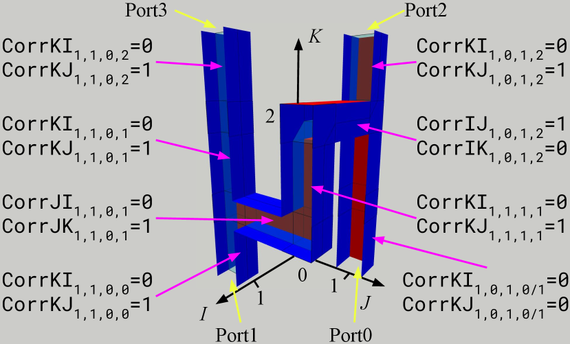
For each stabilizer of a LaS, we need to provide the corresponding correlation surface which can be specified by its pieces inside each pipe. Two pieces are possible inside a pipe: one that connects the two blue faces and one that connects the two red faces. Thus, we need two bits per pipe for each of the correlation surfaces. These are the Corr** variables below. There are six arrays of correlation surface variables, each has shape ($n_{\text{stab}}$, max_i, max_j, max_k), one binary variable per stabilizer per volume. Fig. 10 provides the correlation surface variable values in each pipe for the surface seen in Fig. 6a.

$\texttt{CorrIJ}_{s,i,j,k}$ specifies the existence of correlation surface pieces in the $I$-$J$ plane and inside $I$-pipes. Note that $IZZZ$ has index $s=1$ among the 4 stabilizers, and there is only one $I$-pipe from $(0,1,2)$ to $(1,1,2)$. Thus, $\texttt{CorrIJ}_{1,0,1,2}=1$.

$\texttt{CorrIK}_{s,i,j,k}$ is for correlation surface pieces in the $I$-$K$ plane and inside $I$-pipes. Since there is only one $I$-pipe, the only nontrivial example here is $\texttt{CorrIK}_{1,0,1,2}=0$.

Similarly, we have variable arrays $\texttt{CorrJK}_{s,i,j,k}$ and $\texttt{CorrJI}_{s,i,j,k}$ for correlation surface pieces in $J$-pipes, and $\texttt{CorrKI}_{s,i,j,k}$ and $\texttt{CorrKJ}_{s,i,j,k}$ for those in $K$-pipes. Since each stabilizer needs a different correlation surface, the number of correlation surface variables scales in the product of the volume and the number of stabilizers, much larger than the number of structural variables scaling only in the volume.

Fig. 11 illustrates the constraints for correlation surfaces: two at boundaries (a and d), and two at junctions (b and c).

Stabilizer as Boundary Conditions (Fig. 11a). A stabilizer is specified as Pauli string at the ports, e.g., $IZZZ$ for the four ports of the CNOT. The $Z$ operator touches the two $Z$ boundaries (blue) of the $K$-pipes of the ports. Given that the z-basis-dir in the input is $J$ for all the ports, we find that there should be correlation surface pieces in the $J$-$K$ plane inside the $K$-pipes of ports 1, 2, and 3. Also, the correlation surface pieces corresponding to $X$ operators, in the $K$-$I$ plane, should not be present at these ports. Therefore,

$$\begin{split}&\texttt{CorrKJ}_{1,1,0,0}\ ,\ \ \texttt{CorrKJ}_{1,0,1,2}\ ,\ \ \texttt{CorrKJ}_{1,1,0,2}\ ,\\ &\overline{\texttt{CorrKI}_{1,1,0,0}}\ ,\ \ \overline{\texttt{CorrKI}_{1,0,1,2}}\ ,\ \ \overline{\texttt{CorrKI}_{1,1,0,2}}\ .\end{split}$$

(8)

Port 0 should not have correlation surface pieces in neither direction since in the stabilizer, its term is $I$. If the term for a port is $Y$, then it should have both correlation surface pieces.

Both or None at $Y$ Cubes (Fig. 11d). Since the $Y$ operator is the product of $Z$ and $X$, it correlates the two operators. Thus, two correlation surfaces can end at a $Y$ cube together, or neither of them are present in this region. Per Fig. 9c, only $K$-pipes can connect to $Y$ cubes, so this set of constraint is

$$\texttt{YCube}_{s,i,j,k}\ \Rightarrow\ \big{[}\texttt{CorrKI}_{s,i,j,k}=\texttt{CorrKJ}_{s,i,j,k}\big{]},$$

(9)

for all tuples of $(s,i,j,k)$.

A non-$Y$ and non-port cube can only have degree 2, 3, or 4: degree-1 cube is forbidden by Fig. 9e; and degree-5 or -6 cubes will always contain a 3D corner which is forbidden by Fig. 9d. Degree-2 cubes are “identity” where correlation surfaces trivially travel through. We can neglect them for now and check later that this case is consistent with the two sets of constraints to introduce below. In conclusion, we are only left with degree-3 or -4 cubes which can only be T- or cross-junctions, and they each has a normal direction orthogonal to the plane that draws the T or the cross. In Fig. 11b-c, the T-junctions are in $I$-$J$ plane, so their normal direction is $K$. The two constraints below depend on whether the correlation surfaces are orthogonal or parallel to the normal direction.

Even Parity of Parallel Surfaces at Non-$Y$ Cubes (Fig. 11b, generalizes Fig. 6d-g). There should be an even number of correlation surface pieces parallel to the normal direction of the cube. In Fig. 10, the normal direction for $(0,1,2)$ is $J$, so

$$\begin{split}\big{[}\ &\overline{\texttt{YCube}_{0,1,2}}\ \wedge\overline{\texttt{ExistJ}_{0,0,2}}\ \wedge\overline{\texttt{ExistJ}_{0,1,2}}\ \big{]}\Rightarrow\\ &\big{\{}\big{[}\texttt{ExistI}_{0,1,2}\ \wedge\texttt{CorrIJ}_{1,0,1,2}\big{]}\oplus\big{[}\texttt{ExistK}_{0,1,1}\ \wedge\\ &\ \ \ \texttt{CorrKJ}_{1,0,1,1}\big{]}\oplus\big{[}\texttt{ExistK}_{0,1,2}\wedge\texttt{CorrKJ}_{1,0,1,2}\big{]}=0\big{\}},\end{split}$$

(10)

where the first and third term on the right hand side are 1 because the said correlation surface pieces exist, and the second term is 0 because there is no correlation surface in pipe from $(0,1,1)$ to $(0,1,2)$. Although it is in general costly to express parity operator with first-order logic, we are only dealing with three or four terms, so the translation is simple.

All or No Orthogonal Surfaces at Non-$Y$ Cubes (Fig. 11c, generalizes Fig. 6b-c). The correlation surface pieces orthogonal to the normal direction at a cube should all be present or all missing. Let us consider $(1,0,1)$ with normal direction $I$:

$$\begin{split}&\big{[}\ \overline{\texttt{YCube}_{1,0,1}}\ \wedge\overline{\texttt{ExistI}_{0,0,1}}\ \wedge\overline{\texttt{ExistI}_{1,0,1}}\ \big{]}\Rightarrow\\ &\ \big{\{}\big{[}\ \overline{\texttt{ExistJ}_{1,0,1}}\ \vee\texttt{CorrJK}_{1,1,0,1}\big{]}\wedge\big{[}\ \overline{\texttt{ExistK}_{1,0,0}}\\ &\ \ \vee\texttt{CorrKJ}_{1,1,0,0}\big{]}\wedge\big{[}\ \overline{\texttt{ExistK}_{1,0,1}}\ \vee\texttt{CorrKJ}_{1,1,0,1}\big{]}\big{\}}\bigvee\\ &\ \big{\{}\big{[}\ \overline{\texttt{ExistJ}_{1,0,1}}\ \vee\overline{\texttt{CorrJK}_{1,1,0,1}}\ \big{]}\wedge\big{[}\ \overline{\texttt{ExistK}_{1,0,0}}\\ &\ \ \vee\overline{\texttt{CorrKJ}_{1,1,0,0}}\ \big{]}\wedge\big{[}\ \overline{\texttt{ExistK}_{1,0,1}}\ \vee\overline{\texttt{CorrKJ}_{1,1,0,1}}\ \big{]}\big{\}},\end{split}$$

(11)

where we have two options on the right hand side corresponding to either correlation surface pieces are all present or all missing. In each option, there are three terms corresponding to the three possible pipes connecting $(1,0,1)$. In each term, if the Exist variable is 0, the term trivially evaluates to 1. This corresponds to the fact that if a pipe does not exist, we do not need to consider correlation surface variables inside it.

Generic graph state generation provides a representative scenario for the intended use of LaSsynth. In comparison with the compiler from Ref. [32], tailored for a (logical) 2-lane architecture with careful qubit initialization and optimal gate scheduling, LaSsynth outperforms this baseline by 56% on average across a comprehensive 8-qubit graph state benchmark set, as shown in Fig. 13. Our advantage lies in the smaller footprint per logical qubit, coupled with the ability to establish more intricate connectivity for accessing them.

We can utilize LaSsynth to construct non-Clifford LaS by inputting non-Clifford resource from ports. For instance, in the majority gate, an important LaS in Shor’s algorithm, three ports consume a $|$CCZ$\rangle$. LaSsynth reduces volume by 40% compared to the design in Ref. [20]. The corresponding ZX diagram is challenging for human understanding because of the creative use of generalized Hopf rule (see Fig. 15). Our ZX calculus verification reaffirms the correctness of our result and actually reveals the error of the design in Ref. [20].

We leverage LaSsynth to optimize $T$-factories, the dominating cost in FTQC. There are some nuanced considerations at the non-Clifford input ports because of nondeterministic state injections. Although we choose to get around these intricacies with very basic techniques, LaSsynth still discovers a 15-to-1 $T$-factory, showcased in Fig. 17, 8% smaller than state-of-the-art design [10, 21]. If neglecting state injection delays, LaSsynth discovers a design, as depicted in Fig. 18b, 18% smaller than the state-of-the-art in this setting [8], using a smaller footprint while maintaining the same depth.

The primary use case for LaSsynth is optimizing critical subroutines. Despite potential exponential scaling of the internal SAT solving, it consistently outperforms human expert designs at the scale of realistically significant subroutines, as evidenced by the presented results. In essence, our advantage lies in more flexibility of allocating, moving, and recycling code patches. As pipe diagrams, the human designs usually let the qubits stay put, i.e., forming “pillars” that vertically goes through the LaS, and lattice surgery is performed by unit-time horizontal crossbars connecting to the pillars. In contrast, the vertical pipes in our generated LaS can terminate and begin at will, so the solver explores a much larger design space, e.g., ancillas may not be immediately recycled, but squeezed and moved around to interact with other qubits.

Graph state. The stabilizers of a graph state with underlying graph $G=(V,E)$ are generated by $\{X_{i}\cdot\prod_{j}Z_{j}\ |\ \forall i\in V,\ (i,j)\in E\}$, i.e., $X$ on a node and $Z$ on all its neighbors in $G$, e.g., Fig. 14a. These states have many applications in FTQC [33, 34]. In fact, any state defined by Pauli string stabilizers is equivalent to a graph state up to single-qubit unitaries, so generic graph state generation serves as the average case of LaS, which is the target use case of our tool.

Hardware assumption. Aligning with the baseline [32], we adopt a (logical) 2-lane architecture. There are 2 lanes of surface code tiles available as workspace, each tile is $d\times d$ physical qubits. In our specification, this means limiting $\texttt{max\_j}=2$. Fig. 14b provides an illustration, where the back lane is for (logical) qubit output, and the front lane is ancillary.

Baseline approach. Liu et al. developed a compiler [32] based on Ref. [8]: initializing logical qubits in selective basis and then performing multi-qubit parity measurements using lattice surgery. They observed that selecting the initialization basis is a Maximum Independent Set problem (MIS). Given the initialization in Fig. 14c, only the last two stabilizers in Fig. 14a require measurement. MIS is NP-hard, so, to be fair, we gave this compiler the same amount of time as LaSsynth spends. In their setting, to enable measurements in both the $X$ and $Z$ bases, the qubits must expose both types of boundaries to the ancilla lane, necessitating 2-tile patches (on the right side of Fig. 14c), pushing footprint of their LaS to 16$\times$2=32.

Comprehensive benchmark set. There are $2^{n(n-1)/2}$ graphs for $n$ nodes, but many of them are equivalent up to 1-Q Cliffords. Our benchmarks are 101 graphs from a database [35] representing all the equivalence classes of 8-qubit graphs.

Our approach. Because of the 2-lane assumption, we specify 8$\times$2 footprint along with the graph state stabilizers to LaSsynth. We initiate the search at a depth 3 and iteratively adjust it based on the response—increasing depth if UNSAT or decreasing it if SAT—to determine the optimal depth. The resulting LaS volume is then 8$\times$2$\times$ the optimal depth.

Source of advantage. The baseline approach relies on 2-tile patches, doubling the required footprint and placing it at a disadvantage. This necessity stems from the limitation of 1-tile patches, where only one basis is exposed to the ancilla at a time, posing a challenge for human intuition to access all required bases effectively. LaSsynth overcomes this limitation by employing domain walls (depicted as yellow rings) and intricate connectivity, as seen in Fig. 14b. In contrast, the baseline solutions would consist only of horizontal bars, i.e., parity measurements, connecting to some of the 8 qubits.

Handling non-Cliffordness. The functionality of LaS is specified by stabilizers, implying it can always be implemented using Clifford gates and Pauli measurements. However, for FTQC, non-Cliffordness like $|T\rangle$ is required, and lattice surgery alone cannot fully implement them. Typically, non-Clifford resources are generated in dedicated regions on the quantum chip and routed to specific places. By considering non-Clifford resources as input to certain ports, the remaining portion constitutes a LaS specified by stabilizers. Thus, our LaS definition is enough for general FTQC subroutines. Additionally, this definition is not limited to specific types of non-Cliffordness; for example, we accommodate the majority gate in Ref. [20], which consumes a $|\text{CCZ}\rangle$ instead of $|T\rangle$.

Port requirements of the majority gate. To align with the use case in Ref. [20] (see Fig. 15a), some port location requirements must be met. Specifically, $t$ and $t^{\prime}$ must be at the same height, so do $a$ and $a^{\prime}$, and $c_{\text{in}}$ and $c_{\text{out}}$. The routed $|\text{CCZ}\rangle$ necessitates three additional vertically aligned ports above them. These constraints imply $\texttt{max\_j}\geq 3$ and $\texttt{max\_k}\geq 5$, leaving the only dimension that can shrink as $I$.

Importance of verification. To verify a design, LaSsynth extracts a ZX diagram, and leverages Stim ZX to derive its stabilizers. When we read off the 5$\times$3$\times$5 design in Ref. [20] to a LaSre and give it to LaSsynth, verification fails, underscoring the susceptibility of human designed LaS to errors and the practical challenges of manual verification, even for experts.

Trying to interpret the generated design. LaSsynth derived a LaS (Fig. 15d) 40% smaller than the baseline. Mechanically following the constraints will not aid interpretation, so we use ZX calculus rewrite rules to prove that the generated LaS is equivalent to the ZX diagram of a majority gate (Fig. 15b). The initial diagram in Fig. 15e is directly extracted from the pipes. In the first step, we apply the Hadamard inversion rule (orange) and the spider-merge rule (magenta). In the second step, we morph the diagram without altering connectivity (numbers annotate corresponding spiders). Next, we apply the (generalized) Hopf rule (green), illustrated in Fig. 15c: when $Z$- and $X$-spiders are connected in a complete bipartite manner, two new spiders can replace them. Applying this rule twice reconstructs the ZX diagram in Fig. 15b, completing our proof. The two Hopf rules significantly alter the connectivity of the diagram, producing a compact yet intricate LaS.

Distillation Factory Motivation. The majority gate consumes non-Cliffordness, but where do those come from? A prevalent solution are magic state distillation factories (usually for $|T\rangle$ or $|\text{CCZ}\rangle$) that consume noisy magic states and produce higher-quality magic states. Our LaS model can support such factories: a first-level factory involves physical magic state injections at certain ports, while a higher-level factory takes already distilled magic states to the ports; the remaining part can still be specified by stabilizers. Distilling an injected $|T\rangle$ to a usable error rate entails thousands of operations, making non-Clifford gates a significant FTQC cost. Reducing distillation factory sizes directly reduces this dominant cost.

The 15-to-1 T-factory baseline. The 15-to-1 $T$-factory is one of the most realistic choices for early FTQC, visualized in Fig. 16b in the circuit model. The 15 $T^{\dagger}$’s and the final output $|T\rangle$ correspond to 16 non-Clifford ports in our LaS. The remaining portion is specified by stabilizers at the locations marked with orange labels, derived in Fig. 16c. A baseline design, manually optimized by experts in Refs. [10, 21], initializes logical qubits in $|0\rangle$ with unit depth, an eigenstate of the $Z$ stabilizers in Fig. 16c. It then measures the 5 8-body $X$ stabilizers in Fig. 16c, each taking unit depth. A layer of possible fixups (see next paragraph) is appended, resulting in a total LaS depth of 6.5. When used repeatedly, one unit of latency is hidden through interleaving, and the baseline factory averages a depth of 5.5. With a footprint of 8$\times$4=32, the baseline factory has an average volume of 32$\times$5.5=176.

Fixups. When injecting $|T\rangle$ in the surface code, half the time yields $|T\rangle$, and the other half yields $|T^{\dagger}\rangle$ [10]. Consequently, we may need to apply an $S$ gate via $Y$ cubes based on the injection result. These dynamic cubes are not included in the formulation since they depend on runtime information. We need to reserve space in the LaS for these cubes. How much space and where is necessary to accommodate any of the $2^{15}$ injection outcomes is an involved topic. For simplicity, we adopt a straightforward technique illustrated in Fig. 17: each injection connects to a $K$-pipe and then bends inward to the rest of the pipe diagram. Fixups for each injection can be attached where the pipe bends. We do not include the fixups to the specification and append the fixup layer after synthesis.

T-factory optimization results. The baseline design actually employs half-distance rotation, not available in our formulation. Despite this disadvantage, by iteratively calling LaSsynth with shrinking volume, we obtained solutions with volumes of 7$\times$5$\times$5=175 and 6$\times$6$\times$4.5=9$\times$4$\times$4.5=162. In Fig. 17, we showcase one of the best designs, 8% smaller than the baseline. We verified its ZX diagram using Stim ZX. Notably, by avoiding half-distance rotations present in the baseline, this design opens opportunities for using half-distance elsewhere. Thus, it is of interest to quantum error correction experts to explore how to reduce the distance in regions of this design, potentially achieving further improvements.

T-factory assuming no classical delay. Much of the preceding discussion delves into fixup details. Ignoring classical injection delay, Ref. [8] presents a 121-volume factory design utilizing 11 patches (Fig. 18c top) and a depth of 11, with four injections from the bottom and the remainder from the side (Fig. 18a). Under the same assumption, LaSsynth derives a design (Fig. 18b) with volume 3$\times$3$\times$11=99, achieving an 18% reduction by using a smaller footprint (Fig. 18c bottom).

Scalability metrics. The runtime of LaSsynth may scale unfavorably due to its dependence on SAT solving. However, its target use case is frequently used subroutines rather than entire algorithms, and the presented results demonstrate its effectiveness in solving significant and realistic subroutines. Some runtimes are recorded in Table I, where the formulation yields a scaling factor, $Vn_{\text{stab}}$, i.e., the volume times the number of stabilizers. It is worth noting that this column may appear slightly larger than expected because of padding layers on boundaries to support ports or non-rectangular floorplans. While the 121-factory has a larger $Vn_{\text{stab}}$ than the 162-factory, it is a simpler problem to solve. A better indicator is the number of variables and clauses of the generated SAT CNF.

Random seed: more is different. There is potential for portfolio-based SAT solving [36]. We employed 10 random seeds on the same CNF, and the standard deviations of the runtimes are presented in the last column of Table I. Notably, for the 162-factory, the runtime difference can be as much as 26 times, indicating that multiple SAT solvers with different seeds may significantly expedite finding a solution.

To UNSAT or not, it is a question. Unsatisfiable specifications took longer than satisfiable ones. In Fig. 13, it is noticeable that long runtimes consistently accompany a ‘spike’ in volume. These instances represent cases where LaSsynth initiates with a depth of 3, requires a relatively lengthy period to determine unsatisfiability, and subsequently discovers a solution with depth 4. Generally, this is the price to pay for the optimality guarantee. For scenarios where optimal solutions are not strictly necessary, prioritizing satisfiability initially—such as with incomplete approaches like MaxSAT, or iterative solving, retaining learned information—can be more beneficial in obtaining good designs efficiently.

References

- [1] P. W. Shor, “Polynomial-time algorithms for prime factorization and discrete logarithms on a quantum computer,” SIAM Review, vol. 41, no. 2, pp. 303–332, 1999, DOI: 10.1137/S0036144598347011.
- [2] Google Quantum AI, “Suppressing quantum errors by scaling a surface code logical qubit,” Nature, vol. 614, no. 7949, pp. 676–681, 2023, DOI: 10.1038/s41586-022-05434-1.
- [3] S. A. Moses, C. H. Baldwin, M. S. Allman, R. Ancona, L. Ascarrunz, C. Barnes, J. Bartolotta, B. Bjork, P. Blanchard, M. Bohn, J. G. Bohnet, N. C. Brown, N. Q. Burdick, W. C. Burton, S. L. Campbell, J. P. Campora, C. Carron, J. Chambers, J. W. Chan, Y. H. Chen, A. Chernoguzov, E. Chertkov, J. Colina, J. P. Curtis, R. Daniel, M. DeCross, D. Deen, C. Delaney, J. M. Dreiling, C. T. Ertsgaard, J. Esposito, B. Estey, M. Fabrikant, C. Figgatt, C. Foltz, M. Foss-Feig, D. Francois, J. P. Gaebler, T. M. Gatterman, C. N. Gilbreth, J. Giles, E. Glynn, A. Hall, A. M. Hankin, A. Hansen, D. Hayes, B. Higashi, I. M. Hoffman, B. Horning, J. J. Hout, R. Jacobs, J. Johansen, L. Jones, J. Karcz, T. Klein, P. Lauria, P. Lee, D. Liefer, S. T. Lu, D. Lucchetti, C. Lytle, A. Malm, M. Matheny, B. Mathewson, K. Mayer, D. B. Miller, M. Mills, B. Neyenhuis, L. Nugent, S. Olson, J. Parks, G. N. Price, Z. Price, M. Pugh, A. Ransford, A. P. Reed, C. Roman, M. Rowe, C. Ryan-Anderson, S. Sanders, J. Sedlacek, P. Shevchuk, P. Siegfried, T. Skripka, B. Spaun, R. T. Sprenkle, R. P. Stutz, M. Swallows, R. I. Tobey, A. Tran, T. Tran, E. Vogt, C. Volin, J. Walker, A. M. Zolot, and J. M. Pino, “A race-track trapped-ion quantum processor,” Phys. Rev. X, vol. 13, p. 041052, 2023, DOI: 10.1103/PhysRevX.13.041052.
- [4] A. R. Calderbank, E. M. Rains, P. M. Shor, and N. J. Sloane, “Quantum error correction via codes over GF(4),” IEEE Transactions on Information Theory, vol. 44, no. 4, pp. 1369–1387, 1998, DOI: 10.1109/ISIT.1997.613213.
- [5] E. Dennis, A. Kitaev, A. Landahl, and J. Preskill, “Topological quantum memory,” Journal of Mathematical Physics, vol. 43, no. 9, pp. 4452–4505, 2002, DOI: 10.1063/1.1499754.
- [6] D. Gottesman, “Stabilizer codes and quantum error correction,” Ph.D. dissertation, California Institute of Technology, 1997, DOI: 10.48550/arXiv.quant-ph/9705052.
- [7] A. G. Fowler, M. Mariantoni, J. M. Martinis, and A. N. Cleland, “Surface codes: Towards practical large-scale quantum computation,” Phys. Rev. A, vol. 86, p. 032324, 2012, DOI: 10.1103/PhysRevA.86.032324.
- [8] D. Litinski, “A game of surface codes: Large-scale quantum computing with lattice surgery,” Quantum, vol. 3, p. 128, 2019, DOI: 10.22331/q-2019-03-05-128.
- [9] D. Litinski and N. Nickerson, “Active volume: An architecture for efficient fault-tolerant quantum computers with limited non-local connections”, 2022, DOI: 10.48550/arXiv.2211.15465.
- [10] A. G. Fowler and C. Gidney, “Low overhead quantum computation using lattice surgery”, 2019, DOI: 10.48550/arXiv.1808.06709.
- [11] D. Horsman, A. G. Fowler, S. Devitt, and R. V. Meter, “Surface code quantum computing by lattice surgery,” New Journal of Physics, vol. 14, no. 12, p. 123011, 2012, DOI: 10.1088/1367-2630/14/12/123011.
- [12] R. Raussendorf, J. Harrington, and K. Goyal, “Topological fault-tolerance in cluster state quantum computation,” New Journal of Physics, vol. 9, no. 6, p. 199, 2007, DOI: 10.1088/1367-2630/9/6/199.
- [13] M. E. Beverland, P. Murali, M. Troyer, K. M. Svore, T. Hoefler, V. Kliuchnikov, G. H. Low, M. Soeken, A. Sundaram, and A. Vaschillo, “Assessing requirements to scale to practical quantum advantage”, 2022, DOI: 10.48550/arXiv.2211.07629.
- [14] C. Chamberland and E. T. Campbell, “Universal quantum computing with twist-free and temporally encoded lattice surgery,” PRX Quantum, vol. 3, p. 010331, 2022, DOI: 10.1103/PRXQuantum.3.010331.
- [15] A. Paler and A. G. Fowler, “OpenSurgery for topological assemblies,” in 2020 IEEE Globecom Workshops, 2020, DOI: 10.1109/GCWkshps50303.2020.9367489.
- [16] G. Watkins, H. M. Nguyen, V. Seshadri, K. Watkins, S. Pearce, H.-K. Lau, and A. Paler, “A high performance compiler for very large scale surface code computations”, 2023, DOI: 10.48550/arXiv.2302.02459.
- [17] S. A. Cuccaro, T. G. Draper, S. A. Kutin, and D. P. Moulton, “A new quantum ripple-carry addition circuit”, 2004, DOI: 10.48550/arXiv.quant-ph/0410184.
- [18] S. Aaronson and D. Gottesman, “Improved simulation of stabilizer circuits,” Phys. Rev. A, vol. 70, p. 052328, 2004, DOI: 10.1103/PhysRevA.70.052328.
- [19] A. Paler, “Design methods for reliable quantum circuits,” Ph.D. dissertation, Universität Passau, 2015.
- [20] C. Gidney and A. G. Fowler, “Flexible layout of surface code computations using AutoCCZ states”, 2019, DOI: 10.48550/arXiv.1905.08916.
- [21] C. Gidney and A. G. Fowler, “Efficient magic state factories with a catalyzed to transformation,” Quantum, vol. 3, p. 135, 2019, DOI: 10.22331/q-2019-04-30-135.
- [22] C. Gidney and M. Ekerå, “How to factor 2048 bit RSA integers in 8 hours using 20 million noisy qubits,” Quantum, vol. 5, p. 433, 2021, DOI: 10.22331/q-2021-04-15-433.
- [23] C. Gidney, “Inplace access to the surface code Y basis,” Quantum, vol. 8, p. 1310, 2024, DOI: 10.22331/q-2024-04-08-1310.
- [24] N. de Beaudrap and D. Horsman, “The ZX calculus is a language for surface code lattice surgery,” Quantum, vol. 4, p. 218, 2020, DOI: 10.22331/q-2020-01-09-218.
- [25] J. van de Wetering, “ZX-calculus for the working quantum computer scientist”, 2020, DOI: 10.48550/arXiv.2012.13966.
- [26] M. Backens, S. Perdrix, and Q. Wang, “A simplified stabilizer ZX-calculus,” Electronic Proceedings in Theoretical Computer Science, vol. 236, pp. 1–20, 2017, DOI: 10.4204/eptcs.236.1.
- [27] H. Bombin, D. Litinski, N. Nickerson, F. Pastawski, and S. Roberts, “Unifying flavors of fault tolerance with the ZX calculus”, 2023, DOI: 10.48550/arXiv.2303.08829.
- [28] L. de Moura and N. Bjørner, “Z3: An efficient SMT solver,” in Tools and Algorithms for the Construction and Analysis of Systems, ser. Lecture Notes in Computer Science, C. R. Ramakrishnan and J. Rehof, Eds. Berlin, Heidelberg: Springer, 2008, pp. 337–340, DOI: 10.1007/978-3-540-78800-3“˙ 24.
- [29] A. Biere and M. Fleury, “Gimsatul, IsaSAT and Kissat entering the SAT Competition 2022,” in Proc. of SAT Competition 2022 – Solver and Benchmark Descriptions, ser. Department of Computer Science Series of Publications B, T. Balyo, M. Heule, M. Iser, M. Järvisalo, and M. Suda, Eds., vol. B-2022-1. University of Helsinki, 2022, pp. 10–11. [Online]. Available: https://cca.informatik.uni-freiburg.de/papers/BiereFleury-SAT-Competition-2022-solvers.pdf
- [30] C. Gidney, “Stim: a fast stabilizer circuit simulator,” Quantum, vol. 5, p. 497, 2021, DOI: 10.22331/q-2021-07-06-497.
- [31] D. B. Tan, “Code for ISCA’24 paper A SAT Scalpel for Lattice Surgery”, 2024, DOI: 10.5281/zenodo.11051465.
- [32] S. Liu, N. Benchasattabuse, D. Q. Morgan, M. Hajdušek, S. J. Devitt, and R. Van Meter, “A substrate scheduler for compiling arbitrary fault-tolerant graph states,” in 2023 IEEE International Conference on Quantum Computing and Engineering (QCE), vol. 01, 2023, pp. 870–880, DOI: 10.1109/QCE57702.2023.00101.
- [33] M. Hein, W. Dür, J. Eisert, R. Raussendorf, M. Van den Nest, and H.-J. Briegel, “Entanglement in graph states and its applications,” in Quantum Computers, Algorithms and Chaos, ser. Proceedings of the Enrico Fermi International School of Physics, vol. 162. Varenna, Italy: IOP Press, 2006, pp. 115–218, DOI: 10.3254/978-1-61499-018-5-115.
- [34] M. K. Vijayan, A. Paler, J. Gavriel, C. R. Myers, P. P. Rohde, and S. J. Devitt, “Compilation of algorithm-specific graph states for quantum circuits,” Quantum Science and Technology, vol. 9, no. 2, p. 025005, feb 2024, DOI: 10.1088/2058-9565/ad1f39.
- [35] A. Cabello, L. E. Danielsen, A. J. López-Tarrida, and J. R. Portillo, “Optimal preparation of graph states,” Phys. Rev. A, vol. 83, p. 042314, 2011, DOI: 10.1103/PhysRevA.83.042314.
- [36] D. Schreiber and P. Sanders, Scalable SAT Solving in the Cloud. Springer, Cham, 07 2021, pp. 518–534, DOI: 10.1007/978-3-030-80223-3“˙ 35.
- [37] D. Herr, F. Nori, and S. J. Devitt, “Lattice surgery translation for quantum computation,” New Journal of Physics, vol. 19, no. 1, p. 013034, 2017, DOI: 10.1088/1367-2630/aa5709.
- [38] D. Litinski, “Magic state distillation: Not as costly as you think,” Quantum, vol. 3, p. 205, 2019, DOI: 10.22331/q-2019-12-02-205.
- [39] A. Paler, S. J. Devitt, and A. G. Fowler, “Synthesis of arbitrary quantum circuits to topological assembly,” Scientific reports, vol. 6, no. 1, p. 30600, 2016, DOI: 10.1038/srep30600.
- [40] A. G. Fowler and S. J. Devitt, “A bridge to lower overhead quantum computation”, 2013, DOI: 10.48550/arXiv.1209.0510.
- [41] C.-H. Hsu, W.-H. Lin, W.-H. Tseng, and Y.-W. Chang, “A bridge-based compression algorithm for topological quantum circuits,” in 2021 58th ACM/IEEE Design Automation Conference (DAC), 2021, pp. 457–462, DOI: 10.1109/DAC18074.2021.9586322.
- [42] Y. Lin, B. Yu, M. Li, and D. Z. Pan, “Layout synthesis for topological quantum circuits with 1-D and 2-D architectures,” IEEE Transactions on Computer-Aided Design of Integrated Circuits and Systems, vol. 37, no. 8, pp. 1574–1587, 2018, DOI: 10.1109/TCAD.2017.2760511.
- [43] F. Hua, Y. Chen, Y. Jin, C. Zhang, A. Hayes, Y. Zhang, and E. Z. Zhang, “AutoBraid: A framework for enabling efficient surface code communication in quantum computing,” in 54th Annual IEEE/ACM International Symposium on Microarchitecture, ser. MICRO ’21. New York, NY, USA: Association for Computing Machinery, 2021, p. 925–936, DOI: 10.1145/3466752.3480072.
- [44] A. Javadi-Abhari, P. Gokhale, A. Holmes, D. Franklin, K. R. Brown, M. Martonosi, and F. T. Chong, “Optimized surface code communication in superconducting quantum computers,” in Proceedings of the 50th Annual IEEE/ACM International Symposium on Microarchitecture, ser. MICRO-50 ’17. New York, NY, USA: Association for Computing Machinery, 2017, p. 692–705, DOI: 10.1145/3123939.3123949.
- [45] S. S. Tannu, Z. A. Myers, P. J. Nair, D. M. Carmean, and M. K. Qureshi, “Taming the instruction bandwidth of quantum computers via hardware-managed error correction,” in Proceedings of the 50th Annual IEEE/ACM International Symposium on Microarchitecture, ser. MICRO-50 ’17. New York, NY, USA: Association for Computing Machinery, 2017, p. 679–691, DOI: 10.1145/3123939.3123940.
- [46] Y. Ding, A. Holmes, A. Javadi-Abhari, D. Franklin, M. Martonosi, and F. T. Chong, “Magic-state functional units: Mapping and scheduling multi-level distillation circuits for fault-tolerant quantum architectures,” in Proceedings of the 51st Annual IEEE/ACM International Symposium on Microarchitecture, ser. MICRO-51. IEEE Press, 2018, p. 828–840, DOI: 10.1109/MICRO.2018.00072.
- [47] N. Shutty and C. Chamberland, “Decoding merged color-surface codes and finding fault-tolerant Clifford circuits using solvers for Satisfiability Modulo Theories,” Physical Review Applied, vol. 18, no. 1, p. 014072, 2022, DOI: 10.1103/PhysRevApplied.18.014072.