A robust approach for generalized linear models based on maximum L$q$-likelihood procedure

The maximum L$q$-likelihood estimator for $\beta$ in the class of generalized linear models is a solution of the estimating equation:

with

corresponds to the weight arising from the estimation function defined in (1.4), with $c_{q}(y_{i},\phi)=(1-q)c(y_{i},\phi)$, while $\mu_{i}=\operatorname{E}(y_{i})=\dot{b}(\theta_{i})$, $\operatorname{var}(y_{i})=\phi^{-1}V_{i}$, with $V_{i}=\ddot{b}(\theta_{i})$ being the variance function, and $W_{i}=V_{i}\{\dot{k}(\eta_{i})\}^{2}$, we shall use dots over functions to denote derivatives, $\dot{k}(u)={\operatorname{d}}k/{\operatorname{d}}u$ and $\ddot{k}(u)={\operatorname{d}}^{2}k/{\operatorname{d}}u^{2}$. In this paper, we consider $q<1$ in which case the weights $U_{i}(\mbox{\boldmath$\beta$})$ $(i=1\dots,n)$ provide a mechanism for downweighting outlying observations. The individual score function adopts the form $\mbox{\boldmath$s$}_{i}(\mbox{\boldmath$\beta$})=\phi W_{i}^{1/2}r_{i}\mbox{\boldmath$x$}_{i}$, where $r_{i}=(y_{i}-\mu_{i})/\sqrt{V_{i}}$ denotes the Pearson residual. It is straightforward to notice that the estimation function for $\beta$ can be written as:

where $\mbox{\boldmath$U$}=\operatorname{diag}(U_{1},\dots,U_{n})$, with $U_{i}=U_{i}(\mbox{\boldmath$\beta$})$ is given in (2.2), while $\mbox{\boldmath$W$}=\operatorname{diag}(W_{1},\dots,W_{n})$, $\mbox{\boldmath$V$}=\operatorname{diag}(V_{1},\dots,V_{n})$, $\mbox{\boldmath$Y$}=(y_{1},\dots,y_{n})^{\top}$ and $\mbox{\boldmath$\mu$}=(\mu_{1},\dots,\mu_{n})^{\top}$.

In Appendix A we show that the estimating function in (2.1) is unbiased for the surrogate parameter $\mbox{\boldmath$\beta$}_{*}$, that is $\operatorname{E}_{0}\{\mbox{\boldmath$\Psi$}_{n}(\mbox{\boldmath$\beta$}_{*})\}=\mbox{\boldmath$0$}$, where $\operatorname{E}_{0}(\cdot)$ denotes expectation with respect to the true distribution $f(\cdot;\theta_{0},\phi)$. Thereby, this allows introducing a suitable calibration function, say $\tau_{q}(\cdot)$, such that $\widehat{\mbox{\boldmath$\beta$}}_{q}=\tau_{q}(\widehat{\mbox{\boldmath$\beta$}}{}_{q}^{*})$ which is applied to rescale the parameter estimates in order to achieve Fisher-consistency for $\mbox{\boldmath$\beta$}_{0}$.

When partial derivatives and expectations exist, we define the matrices

where $\mbox{\boldmath$J$}=\operatorname{diag}(J_{1},\dots,J_{n})$ whose diagonal elements are given by $J_{i}=J_{q}^{-\phi}(\theta_{i})$, for $i=1,\dots,n$, with $J_{q}(\theta)=\exp\{-qb(\theta)+b(q\theta)\}$, $q\theta\in\Theta$ was defined by Menendez (2000), whereas $\mbox{\boldmath$G$}=\operatorname{diag}(\dot{g}(\theta_{1}^{*}),\dots,\dot{g}(\theta_{n}^{*}))$ and $\mbox{\boldmath$K$}=\operatorname{diag}(\dot{k}(\eta_{1}),\dots,\dot{k}(\eta_{n}))$ with ${\operatorname{d}}\eta_{*}/{\operatorname{d}}\eta=(1/q)\dot{g}(\theta_{*})\dot{k}(\eta)$ and $g(\theta_{*})=k^{-1}(\theta_{*})$ corresponding to the inverse function of the $\theta$-link evaluated on the surrogate parameter. We propose to use the Newton-scoring algorithm (Jørgensen and Knudsen, 2004) to address the parameter estimation associated with the estimating equation $\mbox{\boldmath$\Psi$}_{n}(\mbox{\boldmath$\beta$})=\mbox{\boldmath$0$}$, which assumes the form

Therefore, the estimation procedure adopts an iteratively reweighted least squares structure, as

where $\mbox{\boldmath$Z$}_{q}=\mbox{\boldmath$\eta$}+\mbox{\boldmath$J$}^{-1}\mbox{\boldmath$G$}^{-1}\mbox{\boldmath$K$}^{-1}\mbox{\boldmath$W$}^{-1/2}\mbox{\boldmath$UV$}^{-1/2}(\mbox{\boldmath$Y$}-\mbox{\boldmath$\mu$})$ denotes the working response which must be evaluated at $\mbox{\boldmath$\beta$}=\mbox{\boldmath$\beta$}^{(t)}$. Let $\widehat{\mbox{\boldmath$\beta$}}{}_{q}^{*}$ be the value obtained at the convergence of the algorithm in (2.5). Thus, in order to obtain a corrected version of the maximum L$q$-likelihood estimator, we must take

Evidently, for the canonical $\theta$-link, $k(u)=u$, it is sufficient to consider $\widehat{\mbox{\boldmath$\eta$}}_{q}=q\widehat{\mbox{\boldmath$\eta$}}{}_{q}^{*}$, or equivalently $\widehat{\mbox{\boldmath$\beta$}}_{q}=q\widehat{\mbox{\boldmath$\beta$}}{}_{q}^{*}$. In addition, for this case we have $\mbox{\boldmath$GK$}=\mbox{\boldmath$I$}_{n}$, with $\mbox{\boldmath$I$}_{n}$ being the identity matrix of order $n$, which leads to a considerably simpler version of the algorithm proposed in (2.5). Qin and Priebe (2017) suggested another alternative to achieve Fisher-consistency which is based on re-centering the estimation equation, considering a bias-correction term, and who termed it as the bias-corrected maximum L$q$-likelihood estimator. We emphasize the simplicity of the calibration function in (2.6), which introduces a reparameterization that allows us to characterize the asymptotic distribution of $\widehat{\mbox{\boldmath$\beta$}}_{q}$.

The following result describes the asymptotic normality of the $\widehat{\mbox{\boldmath$\beta$}}_{q}$ estimator in the context of generalized linear models.

From the general theory of robustness, we can characterize a slight misspecification of the proposed model by the influence function of a statistical functional $\mbox{\boldmath$T$}(F)$, which is defined as (see Hampel et al., 1986, Sec. 4.2),

where $F_{\epsilon}=(1-\epsilon)F+\epsilon\delta_{Y}$, with $\delta_{Y}$ a point mass distribution in $Y$. That is, $\operatorname{IF}(Y;\mbox{\boldmath$T$})$ reflects the effect on $T$ of a contamination by adding an observation in $Y$. It should be noted that the maximum L$q$-likelihood estimation procedure for $q$ fixed corresponds to an $M$-estimation method, where $q$ acts as a tuning constant. It is well known that the influence functions of the estimators obtained by the maximum likelihood and L$q$-likelihood methods adopt the form

respectively, where $\mbox{\boldmath$\mathcal{F}$}_{n}=\operatorname{E}\{-\partial\mbox{\boldmath$s$}_{n}(\mbox{\boldmath$\beta$})/\partial\mbox{\boldmath$\beta$}^{\top}\}=\phi^{-1}\mbox{\boldmath$X$}^{\top}\mbox{\boldmath$WX$}$ is the Fisher information matrix, with $\mbox{\boldmath$s$}_{n}(\mbox{\boldmath$\beta$})=\sum_{i=1}^{n}\mbox{\boldmath$s$}_{i}(\mbox{\boldmath$\beta$})$ the score function, whereas $\{f(y;k(\mbox{\boldmath$x$}^{\top}\mbox{\boldmath$\beta$}),\phi)\}^{1-q}$ corresponds to the weighting defined in (2.2) and $\mbox{\boldmath$s$}(\mbox{\boldmath$\beta$})=\phi W^{1/2}(y-\mu)\mbox{\boldmath$x$}/\sqrt{V}$, with $\mbox{\boldmath$x$}=(x_{1},\dots,x_{p})^{\top}$. It is possible to appreciate that when $q<1$ the weights $U_{i}(\mbox{\boldmath$\beta$})$ provide a mechanism to limit the influence of extreme observations. This allows downweighting those observations that are strongly discrepant from the proposed model. The properties of robust procedures based on the weighting of observations using the working statistical model have been discussed, for example in Windham (1995) and Basu et al. (1998), who highlighted the connection between these procedures with robust methods (see also, Ferrari and Yang, 2010). Indeed, we can write the asymptotic covariance of $\widehat{\mbox{\boldmath$\beta$}}_{q}$ equivalently as,

Additionally, it is known that $\mbox{\boldmath$B$}_{n}^{-1}\mbox{\boldmath$A$}_{n}\mbox{\boldmath$B$}_{n}^{-1}-\mbox{\boldmath$\mathcal{F}$}_{n}^{-1}$, is a positive semidefinite matrix. That is, the $\widehat{\mbox{\boldmath$\beta$}}_{q}$ estimator has asymptotic covariance matrix always larger than the covariance of $\widehat{\mbox{\boldmath$\beta$}}_{\mathrm{ML}}$ for the working model defined in (1.1) and (1.2). To quantify the loss in efficiency of the maximum L$q$-likelihood estimator, is to consider the asymptotic relative efficiency of $\widehat{\mbox{\boldmath$\beta$}}_{q}$ with respect to $\widehat{\mbox{\boldmath$\beta$}}_{\mathrm{ML}}$, which is defined as,

Hence, $\operatorname{ARE}(\widehat{\mbox{\boldmath$\beta$}}_{q},\widehat{\mbox{\boldmath$\beta$}}_{\mathrm{ML}})\geq 1$. This leads to a procedure for the selection of the distortion parameter $q$. Following the same reasoning as Windham (1995) an alternative is to choose $q$ from the available data as that $q_{\mathrm{opt}}$ value that minimizes $\operatorname{tr}(\mbox{\boldmath$B$}_{n}^{-1}\mbox{\boldmath$A$}_{n}\mbox{\boldmath$B$}_{n}^{-1})$. In other words, the interest is to select the model for which the loss in efficiency is the smallest. This procedure has also been used in Qin and Priebe (2017) for adaptive selection of the distortion parameter.

In this paper we follow the guidelines given by La Vecchia et al. (2015) who proposed a data-driven method for the selection of $q$ (see also Ribeiro and Ferrari, 2023). In this procedure the authors introduced the concept of stability condition as a mechanism for determining the distortion parameter by considering an equally spaced grid, say $1\geq q_{1}>q_{2}>\cdots>q_{m}$ and for each value in the grid $\widehat{\mbox{\boldmath$\beta$}}_{q_{j}}$, for $j=1,\dots,m$, is computed. To achieve robustness we can select an optimal value $q_{\mathrm{opt}}$, as the greatest value $q_{j}$ satisfying $QV_{j}<\rho$, where $QV_{j}=\|\widehat{\mbox{\boldmath$\beta$}}_{q_{j}}-\widehat{\mbox{\boldmath$\beta$}}_{q_{j+1}}\|$ with $\rho$ a threshold value. Based on experimental results, La Vecchia et al. (2015) proposed to construct a grid between $q_{1}=1$, and some minimum value, $q_{m}$ with increments of 0.01, whereas $\rho=0.05\,\|\widehat{\mbox{\boldmath$\beta$}}_{q_{m}}\|$. One of the main advantages of their procedure is that, in the absence of contamination, it allows to select the distortion parameter as close to 1 as possible, thas is, this leads to the maximum likelihood estimator. Yet another alternative that has shown remarkable performance for $q$-selection based on parametric bootstrap is reported by Giménez et al. (2022a, b).

The goodness of fit in generalized linear models, considering the estimation method based on the L$q$-likelihood function, requires appropriate modifications to obtain robust extensions of the deviance function. Consider the parameter vector to be partitioned as $\mbox{\boldmath$\beta$}=(\mbox{\boldmath$\beta$}_{1}^{\top},\mbox{\boldmath$\beta$}_{2}^{\top})^{\top}$ and suppose that our interest consists of testing the hypothesis $H_{0}:\mbox{\boldmath$\beta$}_{1}=\mbox{\boldmath$0$}$, where $\mbox{\boldmath$\beta$}_{1}\in\mathbb{R}^{r}$. Thus, we can evaluate the discrepancy between the model defined by the null hypothesis versus the model under $H_{1}:\mbox{\boldmath$\beta$}_{1}\neq\mbox{\boldmath$0$}$ using the proposal of Qin and Priebe (2017), as

where $\widehat{\mbox{\boldmath$\beta$}}_{q}$ and $\widetilde{\mbox{\boldmath$\beta$}}_{q}$ are the corrected maximum L$q$-likelihood estimates for $\beta$ obtained under $H_{0}$ and $H_{1}$, respectively, and using these estimates we have that $\widetilde{\mu}_{i}=\mu_{i}(\widetilde{\mbox{\boldmath$\beta$}}_{q})$ and $\widehat{\mu}_{i}=\mu_{i}(\widehat{\mbox{\boldmath$\beta$}}_{q})$, for $i=1,\dots,n$. Qin and Priebe (2017) based on results available in Cantoni and Ronchetti (2001), proved that the $D_{q}(\mbox{\boldmath$Y$},\widehat{\mbox{\boldmath$\mu$}})$ statistic has an asymptotic distribution following a discrete mixture of chi-squared random variables with one degree of freedom. We should note that the correction term proposed in Qin and Priebe (2017) in our case zeroed for the surrogate parameter.

Following Ronchetti (1997), we can introduce the Akaike information criterion based on the L$q$-estimation procedure, as follows

where $\widehat{\mbox{\boldmath$\beta$}}_{q}$ corresponds to the maximum L$q$-likelihood estimator obtained from the algorithm defined in (2.5). Using the definitions of $\mbox{\boldmath$A$}_{n}$ and $\mbox{\boldmath$B$}_{n}$, given in (2.3) and (2.4) leads to,

Evidently, when the canonical $\theta$-link is considered, we obtain that the penalty term assumes the form $2\operatorname{tr}(\widehat{\mbox{\boldmath$B$}}_{n}^{-1}\widehat{\mbox{\boldmath$A$}}_{n})=2p/(2-q)$ and in the case that $q\to 1$ we recover the usual Akaike information criterion, $\operatorname{AIC}$ for model selection in the context of maximum likelihood estimation. Some authors (see for instance, Ghosh and Basu, 2016), have suggested using the Akaike information criterion $\operatorname{AIC}_{q}$ as an alternative mechanism for the selection of the tuning parameter, i.e., the distortion parameter $q$.

A robust alternative for conducting hypothesis testing in the context of maximum L$q$-likelihood estimation has been proposed by Qin and Priebe (2017), who studied the properties of L$q$-likelihood ratio type statistics for simple hypotheses. As suggested in Equation (3.1) this type of development allows, for example, the evaluation of the fitted model. In this section we focus on testing linear hypotheses of the type

where $H$ es a known matrix of order $d\times p$, with $\operatorname{rank}(\mbox{\boldmath$H$})=d$ $(d\leq p)$ and $\mbox{\boldmath$h$}\in\mathbb{R}^{d}$. Wald, score-type and bilinear form (Crudu and Osorio, 2020) statistics for testing the hypothesis in (3.2) are given by the following result.

Robustness of the statistics defined in (3.3)-(3.5) can be characterized using the tools available in Heritier and Ronchetti (1994). In addition, it is relatively simple to extend these test statistics to manipulate nonlinear hypotheses following the results developed by Crudu and Osorio (2020).

Suppose that our aim is to evaluate the inclusion of a new variable in the regression model. Following Wang (1985), we can consider the added-variable model, which is defined through the linear predictor $\eta_{i}=\mbox{\boldmath$x$}_{i}^{\top}\mbox{\boldmath$\beta$}+z_{i}\gamma=\mbox{\boldmath$f$}_{i}^{\top}\mbox{\boldmath$\delta$}$, where $\mbox{\boldmath$f$}_{i}^{\top}=(\mbox{\boldmath$x$}_{i}^{\top},z_{i})$ and $\mbox{\boldmath$\delta$}=(\mbox{\boldmath$\beta$}^{\top},\gamma)^{\top}$, with $\theta_{i}=k(\eta_{i})$, for $i=1,\dots,n$. Based on the above results we present the score-type statistic for testing the hypothesis $H_{0}:\gamma=0$. Let $\mbox{\boldmath$F$}=(\mbox{\boldmath$X$},\mbox{\boldmath$z$})$ be the model matrix for the added-variable model, with $\mbox{\boldmath$X$}=(\mbox{\boldmath$x$}_{1},\dots,\mbox{\boldmath$x$}_{n})^{\top}$ and $\mbox{\boldmath$z$}=(z_{1},\dots,z_{n})^{\top}$. That notation, enables us to write the estimation function associated with the maximum L$q$-likelihood estimation problem as:

whereas,

It is easy to notice that the estimate for $\beta$ under the null hypothesis, $H_{0}:\gamma=0$ can be obtained by the Newton-scoring algorithm given in (2.5). Details of the derivation of the score-type statistic for testing $H_{0}:\gamma=0$ are deferred to Appendix E, where it is obtained

which for the context of the added variable model, takes the form:

where $\mbox{\boldmath$P$}=\mbox{\boldmath$X$}(\mbox{\boldmath$X$}^{\top}\mbox{\boldmath$WJGKX$})^{-1}\mbox{\boldmath$X$}^{\top}$. Thus, we reject the null hypothesis by comparing the value obtained for $R_{n}$ with some percentile value $(1-\alpha)$ of the chi-squared distribution with one degree of freedom. This type of development has been used, for example, in Wei and Shih (1994) to propose tools for outlier detection considering the mean-shift outlier model in both generalized linear and nonlinear regression models for the maximum likelihood framework. It should be noted that the mean-shift outlier model can be obtained by considering $\mbox{\boldmath$z$}=(0,\dots,1,\dots,0)^{\top}$ as the vector of zeros except for an 1 at the $i$th position, which leads to the standardized residual.

where $\widehat{U}_{i}=U_{i}(\widehat{\mbox{\boldmath$\beta$}})$, $\widehat{J}_{i}=J_{q}^{-\phi}(\theta_{i}(\widehat{\mbox{\boldmath$\beta$}}))$, $\widehat{g}_{i}=\dot{g}(\widehat{\theta}_{i}^{*})$, $\widehat{k}_{i}=\dot{k}(\widehat{\eta}_{i})$, and $\widehat{m}_{ii}$, $\widehat{m}_{ii}^{*}$ are, respectively, the diagonal elements of matrices $\widehat{\mbox{\boldmath$M$}}=\widehat{\mbox{\boldmath$P$}}\widehat{\mbox{\boldmath$W$}}\widehat{\mbox{\boldmath$J$}}$ and $\widehat{\mbox{\boldmath$M$}}{}^{2}$, for $i=1,\dots,n$. It is straightforward to note that $t_{i}$ has an approximately standard normal distribution and can be used for the identification of outliers and possibly influential observations. Evidently, we have that for $q=1$ we recover the standardized residual for generalized linear models. We have developed the standardized residual, $t_{i}$ based on the type-score statistic defined based on (3.4), further alternatives for standardized residuals can be constructed by using the Wald and bilinear-form statistics defined in Equations (3.3) and (3.5), respectively. Additionally, we can consider other types of residuals. Indeed, based on Equation (3.1) we can define the deviance residual as,

with $d(y_{i},\widehat{\mu}_{i})=2\{l_{q}(y_{i},\widehat{\mu}_{i})-l_{q}(y_{i},y_{i})\}$, the deviance associated with the $i$th observation. Moreover, it is also possible to consider the quantile residual (Dunn and Smyth, 1996), which is defined as

where $F(\cdot;\mu,\phi)$ is the cumulative distribution function associated with the random variable $y$, while $\Phi(\cdot)$ is the cumulative distribution function of the standard normal.

Throughout this work we have assumed $\phi$ as a fixed niusance parameter. Following Giménez et al. (2022a, b), we can obtain the maximum L$q$-likelihood estimator $\widehat{\phi}_{q}$ by solving the problem,

which corresponds to a profiled L$q$-likelihood function. It should be noted that to obtain $\widehat{\phi}_{q}$ it is sufficient to consider an one-dimensional optimization procedure.

We revisit the dataset introduced by Finney (1947) which aims to assess the effect of the volume and rate of inspired air on transient vasoconstriction in the skin of the digits. The response is binary, indicating the occurrence or non-occurrence of vasoconstriction. Following Pregibon (1981), a logistic regression model using the linear predictor $\eta=\beta_{1}+\beta_{2}\log(\text{volume})+\beta_{3}\log(\text{rate})$, was considered. Observations 4 and 18 have been identified as highly influential on the estimated coefficients obtained by the maximum likelihood method (Pregibon, 1981). In fact, several authors have highlighted the extreme characteristic of this dataset since the removal of these observations brings the model close to indeterminacy (see, for instance Künsch et al., 1989, Sec. 4). Table 4.1, reports the parameter estimates and their standard errors obtained from three robust procedures. Here CR denotes the fit using the method proposed by Cantoni and Ronchetti (2001), BY indicates the estimation method for logistic regression developed by Bianco and Yohai (1996) both available in the robustbase package (Todorov and Filzmoser, 2009) from the R software (R Development Core Team, 2022), while ML$q$, denotes the procedure proposed in this work where we have selected $q$ using the mechanism described in Section 2.2, in which $q=0.79$ was obtained. Furthermore, the results of the maximum likelihood fit are also reported and estimation was carried out using the weighted Bianco and Yohai estimator (Croux and Haesbroeck, 2003). However, since the explanatory variables do not contain any outliers the estimates obtained using BY and weighted BY methods are identical and therefore they are not reported here.

From Table 4.1 we must highlight the drastic change in the estimates of the regression coefficients by maximum likelihood when observations 4 and 18 are deleted (see also Pregibon, 1981; Wang, 1985). It is interesting to note that the results for this case are very close to those offered by the estimation procedure based on the $L_{1}$-norm introduced by Morgenthaler (1992). Moreover, as discussed in Sec. 6.17 of Atkinson and Riani (2000) the removal of observations 4, 18 and 24 leads to a perfect fit. Indeed, the elimination of observations 4 and 18 leads to a huge increment in the standard errors.

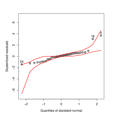
Figure 4.1 (a) shows a strong overlap in the groups with zero and unit response. The poor fit is also evident from the QQ-plot of Studentized residuals with simulated envelopes (see, Figure 4.1 (b)). The estimated weights $\widehat{U}_{i}=U_{i}(\widehat{\mbox{\boldmath$\beta$}})$, $(i=1,\dots,39)$ are displayed in Figure 4.2, where it is possible to appreciate the ability of the algorithm to downweight observations 4, 18 and 24. It should be stressed that the estimation of the regression coefficients by the maximum L$q$-likelihood method with $q=0.79$ is very similar to that obtained by the resistant procedure discussed by Pregibon (1982). Figure 4.3, reveals that the maximum L$q$-likelihood procedure offers a better fit and the QQ-plot with simulated envelope correctly identifies observations 4 and 18 as outliers.

In Appendix F the fit for the proposed model using values ranging from $q=1$ to 0.74, is reported. Table F.1 shows that as the value of $q$ decreases, there is an increase in the standard error of the estimates. Additionally, Figures F.1 and F.2 from Appendix F show how as $q$ decreases the weights of observations 4 and 18 decrease rapidly to zero. Indeed, when $q\leq 0.76$ the problem of indeterminacy underlying these data becomes evident.

To evaluate the performance of the proposed estimation procedure we developed a small Monte Carlo simulation study. We consider a Poisson regression model with logarithmic link function, based on the linear predictor

where $x_{ij}\sim\mathsf{U}(0,1)$ for $j=1,2,3$ and $\mbox{\boldmath$\beta$}=(\beta_{1},\beta_{2},\beta_{3})^{\top}=(1,1,1)^{\top}$. We construct $M=1000$ data sets with sample size $n=25,100$ and $400$ from the model (4.1). Following Cantoni and Ronchetti (2006) the observations are contaminated by multiplying by a factor of $\nu$ a percentage $\varepsilon$ of randomly selected responses. We have considered $\nu=2,5$ and $\varepsilon=0.00,0.05,0.10$ and $0.25$ as contamination percentages. For contaminated as well as non-contaminated data we have carried out the estimation by maximum likelihood, using the method of Cantoni and Ronchetti (2001) and the procedure proposed in this paper.

References

• Atkinson and Riani (2000) Atkinson, A., Riani, M. (2000). Robust Diagnostics Regression Analysis. Springer, New York.
• Basu etย al. (1998) Basu, A., Harris, I.R., Hjort, N.L., Jones, M.C. (1998). Robust and efficient estimation by minimising a density power divergence. Biometrika 85, 549-559.
• Bianco and Yohai (1996) Bianco, A.M., Yohai, V.J. (1996). Robust estimation in the logistic regression model. In: Rieder, H. (Ed.), Robust Statistics, Data Analysis, and Computer Intensive Methods, Lecture Notes in Statistics, Vol. 109. Springer, New York, pp. 17-34.
• Boos (1992) Boos, D.D. (1992). On generalized score tests. The American Statistician 46, 327-333.
• Cantoni and Ronchetti (2001) Cantoni, E., Ronchetti, E. (2001). Robust inference for generalized linear models. Journal of the American Statistical Association 96, 1022-1030.
• Cantoni and Ronchetti (2006) Cantoni, E., Ronchetti, E. (2006). A robust approach for skewed and heavy-tailed outcomes in the analysis of health care expeditures. Journal of Health Economics 25, 198-213.
• Croux and Haesbroeck (2003) Croux, C., Haesbroeck, G. (2003). Implementing the Bianco and Yohai estimator for logistic regression. Computational Statistics and Data Analysis 44, 273-295.
• Crudu and Osorio (2020) Crudu, F., Osorio, F. (2020). Bilinear form test statistics for extremum estimation. Economics Letters 187, 108885.
• Dunn and Smyth (1996) Dunn, P.K., Smyth, G.K. (1996). Randomized quantile residuals. Journal of Computational and Graphical Statistics 5, 236-244.
• Ferrari and Paterlini (2009) Ferrari, D., Paterlini, S. (2009). The maximum Lqq-likelihood method: An application to extreme quantile estimation in finance. Methodology and Computing in Applied Probability 11,3-19.
• Ferrari and Yang (2010) Ferrari, D., Yang, Y. (2010). Maximum Lqq-likelihood estimation. The Annals of Statistics 38, 753-783.
• Finney (1947) Finney, D.J. (1947). The estimation from individual records of the relationships between dose and quantal response. Biometrika 34, 320-324.
• Ghosh and Basu (2016) Ghosh, A., Basu, A. (2016). Robust estimation in generalized linear models: the density power divergence approach. TEST 25, 269-290.
• Gimรฉnez etย al. (2022a) Gimรฉnez, P., Guarracino, L., Galea, M. (2022). Maximum Lqq-likelihood estimation in functional measurement error models. Statistica Sinica 32, 1723-1743.
• Gimรฉnez etย al. (2022b) Gimรฉnez, P., Guarracino, L., Galea, M. (2022). Robust estimation in functional comparative calibration models via maximum Lqq-likelihood. Brazilian Journal of Probability and Statistics 36, 725-750.
• Gourieroux and Monfort (1995) Gourieroux, C. Monfort, A. (1995). Statistics and Econometrics Models: Testing, Confidence Regions, Model Selection and Asymptotic Theory. Vol. 2. Cambridge University Press.
• Green (1984) Green, P.J. (1984). Iteratively reweighted least squares for maximum likelihood estimation, and some robust and resistant alternatives. Journal of the Royal Statistical Society, Series B 46, 149-170.
• Hampel etย al. (1986) Hampel, F.R., Ronchetti, E.M., Rousseeuw, P.J., Stahel, W.A. (1986). Robust Statistics: The approach based on influence functions. Wiley, New York.
• Havrda and Charvรกt (1967) Havrda, J., Charvรกt, F. (1967). Quantification method of classification processes: Concept of structural entropy. Kibernetika 3, 30-35.
• Heritier and Ronchetti (1994) Heritier, S., Ronchetti, E. (1994). Robust bounded-influence tests in general parametric models. Journal of the American Statistical Association 89, 897-904.
• Hosseinian and Morgenthaler (2011) Hosseinian, S., Morgenthaler, S. (2011). Robust binary regression. Journal of Statistical Planning and Inference 141, 1497-1509.
• Huang etย al. (2013) Huang, C., Lin, R., Ren, Y. (2013). Testing for the shape parameter of generalized extreme value distribution based on the Lqq-likelihood estimation ratio statistic. Metrika 76, 641-671.
• Jรธrgensen and Knudsen (2004) Jรธrgensen, B., Knudsen, S.J. (2004). Parameter orthogonality and bias adjustment for estimating functions. Scandinavian Journal of Statistics 31, 93-114.
• Kรผnsch etย al. (1989) Kรผnsch, H.R., Stefanski, L.A., Carroll, R.J. (1989). Conditionally unbiased bounded-influence estimation in general regression models, with applications to generalized linear models. Journal of the American Statistical Association 84, 460-466.
• La Vecchia etย al. (2015) La Vecchia, D., Camponovo, L., Ferrari, D. (2015). Robust heart rate variability analysis by generalized entropy minimization. Computational Statistics and Data Analysis 82, 137-151.
• Menendez (2000) Menendez, M.L. (2000). Shannonโ€™s entropy in exponential families: statistical applications. Applied Mathematics Letters 13, 37-42.
• Morgenthaler (1992) Morgenthaler, S. (1992). Least-absolute-deviations fits for generalized linear models. Biometrika 79, 747-754.
• Nelder and Wedderburn (1972) Nelder, J.A., Wedderburn, R.W.M. (1972). Generalized linear models. Journal of the Royal Statistical Society, Series A 135, 370-384.
• Pregibon (1981) Pregibon, D. (1981). Logistic regression diagnostics. The Annals of Statistics 9, 705-724.
• Pregibon (1982) Pregibon, D. (1982). Resistant fits for some commonly used logistic models with medical applications. Biometrics 38, 485-498.
• Preisser and Qaqish (1999) Preisser, J.S., Qaqish, B.F. (1999). Robust regression for clustered data with applications to binary regression. Biometrics 55, 574-579.
• Qin and Priebe (2013) Qin, Y., Priebe, C.E. (2013). Maximum Lqq-likelihood estimation via the Expectation-Maximization algorithm: A robust estimation of mixture models. Journal of the American Statistical Association 108, 914-928.
• Qin and Priebe (2017) Qin, Y., Priebe, C.E. (2017). Robust hypothesis testing via Lqq-likelihood. Statistica Sinica 27, 1793-1813.
• R Development Core Team (2022) R Development Core Team (2022). R: A Language and Environment for Statistical Computing. Vienna, Austria: R Foundation for Statistical Computing. ISBN 3-900051-07-0, http://www.R-project.org.
• Ribeiro and Ferrari (2023) Ribeiro, T.K.A., Ferrari, S.L.P. (2023). Robust estimation in beta regression via maximum Lqq-likelihood. Statistical Papers 64, 321-353.
• Ronchetti (1997) Ronchetti, E. (1997). Robust aspects of model choice. Statistica Sinica 7, 327-338.
• Stefanski etย al. (1986) Stefanski, L.A., Carroll, R.J., Ruppert, D. (1986). Optimally bounded score functions for generalized linear models with applications to logistic regression. Biometrika 73, 413-425.
• Thomas and Cook (1989) Thomas, W., Cook, R.D. (1989). Assessing influence on regression coefficients in generalized linear models. Biometrika 76, 741-749.
• Thomas and Cook (1990) Thomas, W., Cook, R.D. (1990). Assessing influence on predictions from generalized linear models. Technometrics 32, 59-65.
• Todorov and Filzmoser (2009) Todorov, V., Filzmoser, P. (2009). An object-oriented framework for robust multivariate analysis. Journal of Statistical Software 32 (3), 1-47.
• Tsallis (1988) Tsallis, C. (1988). Possible generalization of Boltzmann-Gibbs statistic. Journal of Statistical Physics 52, 479-487.
• Wang (1985) Wang, P.C. (1985). Adding a variable in generalized linear models. Technometrics 27, 273-276.
• Wei and Shih (1994) Wei, B.C., Shih, J.Q. (1994). On statistical models for regression diagnostics. Annals of the Institute of Statistical Mathematics 46, 267-278.
• Windham (1995) Windham, M.P. (1995). Robustifying model fitting. Journal of the Royal Statistical Society, Series B 57, 599-609.
• Yuan and Jennrich (1998) Yuan, K.H., Jennrich, R.I. (1998). Asymptotics of estimating equations under natural conditions. Journal of Multivariate Analysis 65, 245-260.
Appendix A Fisher consistency
We say that a random variable YY belongs to the exponential family of distributions if its probability density function is given by
fโ€‹(y;ฮธ,ฯ•)=expโก[ฯ•โ€‹{yโ€‹ฮธโˆ’bโ€‹(ฮธ)}+cโ€‹(y,ฯ•)],f(y;\theta,\phi)=\exp[\phi\{y\theta-b(\theta)\}+c(y,\phi)], (A.1)
where bโ€‹(โ‹…)b(\cdot) and cโ€‹(โ‹…,โ‹…)c(\cdot,\cdot) are some specific functions, ฮธ\theta is the natural parameter defined in ฮ˜โŠ‚โ„\Theta\subset\mathbb{R} and ฯ•>0\phi>0 is a dispersion parameter. If a random variable has a density function (A.1), we shall denote Yโˆผ๐–ฅ๐–คโ€‹(ฮธ,ฯ•)Y\sim\mathsf{FE}(\theta,\phi). To verify Fisher consistency, the following Lemma is introduced,
Lemma A.1.
Suppose Yโˆผ๐–ฅ๐–คโ€‹(ฮธ,ฯ•)Y\sim\mathsf{FE}(\theta,\phi) with expectation Eโ€‹(Y)=bห™โ€‹(ฮธ)E(Y)=\dot{b}(\theta), and consider Uโ€‹(ฮธ)={fโ€‹(y;ฮธ,ฯ•)}1โˆ’qU(\theta)=\{f(y;\theta,\phi)\}^{1-q} for q>0q>0. Then, for an integrable function hโ€‹(Y;ฮธ)h(Y;\theta), it follows that
E0โก{Urโ€‹(ฮธ)โ€‹hโ€‹(Y;ฮธ)}=Jqโˆ’ฯ•โ€‹(ฮธ)โ€‹Eqโก{hโ€‹(Y;ฮธ)},\operatorname{E}_{0}\{U^{r}(\theta)h(Y;\theta)\}=J_{q}^{-\phi}(\theta)\operatorname{E}_{q}\{h(Y;\theta)\},
where ฮธ0=qโ€‹ฮธ\theta_{0}=q\theta, and Jqโ€‹(ฮธ)=expโก{โˆ’qโ€‹bโ€‹(ฮธ)+bโ€‹(qโ€‹ฮธ)}J_{q}(\theta)=\exp\{-qb(\theta)+b(q\theta)\} is defined in Menendez (2000), whereas the expectation Eqโก{hโ€‹(Y;ฮธ)}\operatorname{E}_{q}\{h(Y;\theta)\} must be calculated based on the density function
fqโ€‹(y;ฮธ,ฯ•)=expโก[ฯ•โ€‹(rโ€‹(1โˆ’q)+q)โ€‹{yโ€‹ฮธโˆ’bโ€‹(ฮธ)}+cq,rโ€‹(y,ฯ•)],f_{q}(y;\theta,\phi)=\exp[\phi(r(1-q)+q)\{y\theta-b(\theta)\}+c_{q,r}(y,\phi)], (A.2)
and cq,rโ€‹(y,ฯ•)=(rโ€‹(1โˆ’q)+1)โ€‹cโ€‹(y,ฯ•)c_{q,r}(y,\phi)=(r(1-q)+1)c(y,\phi).
Proof.
It is desired to compute expectations of the type
E0โก{Urโ€‹(ฮธ)โ€‹hโ€‹(Y;ฮธ)}=โˆซ๐’ดUrโ€‹(ฮธ)โ€‹hโ€‹(y;ฮธ)โ€‹fโ€‹(y;ฮธ0,ฯ•)โ€‹dy.\operatorname{E}_{0}\{U^{r}(\theta)h(Y;\theta)\}=\int_{\mathcal{Y}}U^{r}(\theta)h(y;\theta)f(y;\theta_{0},\phi){{\rm d}y}.
For ฮธ0=qโ€‹ฮธ\theta_{0}=q\theta, we have
Urโ€‹(ฮธ)โ€‹fโ€‹(y;ฮธ0,ฯ•)=\displaystyle U^{r}(\theta)f(y;\theta_{0},\phi)={} {fโ€‹(y;ฮธ,ฯ•)}rโ€‹(1โˆ’q)โ€‹fโ€‹(y;qโ€‹ฮธ,ฯ•)\displaystyle\{f(y;\theta,\phi)\}^{r(1-q)}f(y;q\theta,\phi)
=\displaystyle={} expโก[rโ€‹(1โˆ’q)โ€‹ฯ•โ€‹{yโ€‹ฮธโˆ’bโ€‹(ฮธ)}+rโ€‹(1โˆ’q)โ€‹cโ€‹(y;ฯ•)]\displaystyle\exp[r(1-q)\phi\{y\theta-b(\theta)\}+r(1-q)c(y;\phi)]
ร—expโก[ฯ•โ€‹{yโ€‹qโ€‹ฮธโˆ’bโ€‹(qโ€‹ฮธ)}+cโ€‹(y,ฯ•)].\displaystyle\times\exp[\phi\{yq\theta-b(q\theta)\}+c(y,\phi)].
It is easy to notice that
r(1โˆ’q)ฯ•{yฮธ\displaystyle r(1-q)\phi\{y\theta โˆ’b(ฮธ)}+ฯ•{yqฮธโˆ’b(qฮธ)}\displaystyle-b(\theta)\}+\phi\{yq\theta-b(q\theta)\}
=ฯ•โ€‹(rโ€‹(1โˆ’q)+q)โ€‹{yโ€‹ฮธโˆ’bโ€‹(ฮธ)}+ฯ•โ€‹{qโ€‹bโ€‹(ฮธ)โˆ’bโ€‹(qโ€‹ฮธ)}.\displaystyle=\phi(r(1-q)+q)\{y\theta-b(\theta)\}+\phi\{qb(\theta)-b(q\theta)\}.
Thus,
Urโ€‹(ฮธ)โ€‹fโ€‹(y;ฮธ0,ฯ•)=expโก[ฯ•โ€‹{qโ€‹bโ€‹(ฮธ)โˆ’bโ€‹(qโ€‹ฮธ)}]โ€‹expโก[ฯ•โ€‹(rโ€‹(1โˆ’q)+q)โ€‹{yโ€‹ฮธโˆ’bโ€‹(ฮธ)}+cqโ€‹(y;ฯ•)],U^{r}(\theta)f(y;\theta_{0},\phi)=\exp[\phi\{qb(\theta)-b(q\theta)\}]\exp[\phi(r(1-q)+q)\{y\theta-b(\theta)\}+c_{q}(y;\phi)],
where cqโ€‹(y,ฯ•)=(rโ€‹(1โˆ’q)+1)โ€‹cโ€‹(y,ฯ•)c_{q}(y,\phi)=(r(1-q)+1)c(y,\phi) and let
Jqโ€‹(ฮธ)=expโก{โˆ’qโ€‹bโ€‹(ฮธ)+bโ€‹(qโ€‹ฮธ)},qโ€‹ฮธโˆˆฮ˜,J_{q}(\theta)=\exp\{-qb(\theta)+b(q\theta)\},\qquad q\theta\in\Theta,
(see Menendez, 2000), which leads to write
E0โก{Urโ€‹(ฮธ)โ€‹hโ€‹(Y;ฮธ)}=Jqโˆ’ฯ•โ€‹(ฮธ)โ€‹Eqโก{hโ€‹(Y,ฮธ)},\operatorname{E}_{0}\{U^{r}(\theta)h(Y;\theta)\}=J_{q}^{-\phi}(\theta)\operatorname{E}_{q}\{h(Y,\theta)\},
because Eqโ€‹{hโ€‹(Y,ฮธ)}=โˆซ๐’ดhโ€‹(y;ฮธ)โ€‹fqโ€‹(y;ฮธ,ฯ•)โ€‹dyE_{q}\{h(Y,\theta)\}=\int_{\mathcal{Y}}h(y;\theta)f_{q}(y;\theta,\phi){{\rm d}y}, with fqโ€‹(y;ฮธ,ฯ•)f_{q}(y;\theta,\phi) as defined in (A.2). โˆŽ
Proposition A.2.
The estimation function defined in Equation (2.1) is unbiased for the surrogate parameter ฮธโˆ—=ฮธ0/q\theta_{*}=\theta_{0}/q.
We have to calculate the expectation,
E0โก{๐šฟnโ€‹(๐œทโˆ—)}=ฯ•โ€‹โˆ‘i=1nWi1/2โ€‹E0โก{Uiโ€‹(๐œทโˆ—)โ€‹(Yiโˆ’ฮผโˆ—,i)}Viโ€‹๐’™i.\operatorname{E}_{0}\{\mbox{\boldmath$\Psi$}_{n}(\mbox{\boldmath$\beta$}_{*})\}=\phi\sum_{i=1}^{n}W_{i}^{1/2}\frac{\operatorname{E}_{0}\{U_{i}(\mbox{\boldmath$\beta$}_{*})(Y_{i}-\mu_{*,i})\}}{\sqrt{V_{i}}}\mbox{\boldmath$x$}_{i}.
Since Uiโ€‹(๐œทโˆ—)={fโ€‹(yi;ฮธiโ€‹(๐œทโˆ—),ฯ•)}1โˆ’qU_{i}(\mbox{\boldmath$\beta$}_{*})=\{f(y_{i};\theta_{i}(\mbox{\boldmath$\beta$}_{*}),\phi)\}^{1-q}, it is enough to obtain E0โก{Uโ€‹(ฮธโˆ—)โ€‹(Yโˆ’ฮผโˆ—)}\operatorname{E}_{0}\{U(\theta_{*})(Y-\mu_{*})\}. Using Lemma A.1, leads to
E0โก{Uโ€‹(ฮธโˆ—)โ€‹(Yโˆ’ฮผโˆ—)}=Jqโˆ’ฯ•โ€‹(ฮธโˆ—)โ€‹Eqโก(Yโˆ’ฮผโˆ—).\operatorname{E}_{0}\{U(\theta_{*})(Y-\mu_{*})\}=J_{q}^{-\phi}(\theta_{*})\operatorname{E}_{q}(Y-\mu_{*}).
Noticing that
Eqโก(Yโˆ’ฮผโˆ—)=โˆซ๐’ด{yโˆ’bห™โ€‹(ฮธโˆ—)}โ€‹fqโ€‹(y;ฮธโˆ—,ฯ•)โ€‹dy=0,\operatorname{E}_{q}(Y-\mu_{*})=\int_{\mathcal{Y}}\{y-\dot{b}(\theta_{*})\}f_{q}(y;\theta_{*},\phi){{\rm d}y}=0,
yields E0โก{๐šฟnโ€‹(๐œทโˆ—)}=0\operatorname{E}_{0}\{\mbox{\boldmath$\Psi$}_{n}(\mbox{\boldmath$\beta$}_{*})\}=0. That is, it is an unbiased estimation function for ฮธโˆ—\theta_{*}. โˆŽ
Appendix B Corrected version of the maximum Lqq-likelihood estimator in GLM
Let ฮธ0\theta_{0} be the true parameter, Ferrari and Yang (2010) highlighted that for qq fixed, the maximum Lqq-likelihood estimator ฮธ^qโˆ—\hat{\theta}_{q}^{*} converges in probability to ฮธโˆ—=ฮธ0/q\theta_{*}=\theta_{0}/q. Here, ฮธโˆ—\theta_{*} is called the surrogate parameter of ฮธ0\theta_{0}. This leads to the correction ฮธ^q=qโ€‹ฮธ^qโˆ—โ†’pqโ€‹ฮธโˆ—=ฮธ0\hat{\theta}_{q}=q\hat{\theta}_{q}^{*}\stackrel{{\scriptstyle p}}{{\to}}q\theta_{*}=\theta_{0}. Considering the ฮธ\theta-link, that is ฮธ=kโ€‹(ฮท)\theta=k(\eta), we write ๐œผโˆ—=kโˆ’1โ€‹(๐œฝโˆ—)=๐‘ฟโ€‹๐œทโˆ—\mbox{\boldmath$\eta$}_{*}=k^{-1}(\mbox{\boldmath$\theta$}_{*})=\mbox{\boldmath$X\beta$}_{*} for the corresponding surrogates. Then we have that
ฮท^q=kโˆ’1โ€‹(qโ€‹ฮธ^qโˆ—)โ†’pkโˆ’1โ€‹(ฮธ0)=ฮท0.\hat{\eta}_{q}=k^{-1}(q\hat{\theta}_{q}^{*})\stackrel{{\scriptstyle p}}{{\to}}k^{-1}(\theta_{0})=\eta_{0}.
This leads to the following correction for the linear predictor ฮท^q=kโˆ’1โ€‹(qโ€‹kโ€‹(ฮท^qโˆ—))\hat{\eta}_{q}=k^{-1}(qk(\hat{\eta}_{q}^{*})), which yields the calibration function in Equation (2.6).
Appendix C Asymptotic covariance
Previous to the calculation of matrices defined in Equations (2.3) and (2.4), we introduce the following Lemma.
Lemma C.1.
Consider Yโˆผ๐–ฅ๐–คโ€‹(ฮธ,ฯ•)Y\sim\mathsf{FE}(\theta,\phi) and assume the elements given in Lemma A.1. Therefore it is straightforward that
E0โก{Urโ€‹(ฮธ)โ€‹(Yโˆ’ฮผ)2}=ฯ•โˆ’1rโ€‹(1โˆ’q)+qโ€‹Jqโˆ’ฯ•โ€‹(ฮธ)โ€‹Vโ€‹(ฮผ),\operatorname{E}_{0}\{U^{r}(\theta)(Y-\mu)^{2}\}=\frac{\phi^{-1}}{r(1-q)+q}J_{q}^{-\phi}(\theta)V(\mu),
where Vโ€‹(ฮผ)=bยจโ€‹(ฮธ)V(\mu)=\ddot{b}(\theta) is the variance function.
Using Lemma A.1, we have that E0โก{Urโ€‹(ฮธ)โ€‹(Yโˆ’ฮผ)2}=Jqโˆ’ฯ•โ€‹(ฮธ)โ€‹Eqโก{(Yโˆ’ฮผ)2}\operatorname{E}_{0}\{U^{r}(\theta)(Y-\mu)^{2}\}=J_{q}^{-\phi}(\theta)\operatorname{E}_{q}\{(Y-\mu)^{2}\}. Since,
Eqโก{(Yโˆ’ฮผ)2}=ฯ•โˆ’1rโ€‹(1โˆ’q)+qโ€‹bยจโ€‹(ฮธ),\operatorname{E}_{q}\{(Y-\mu)^{2}\}=\frac{\phi^{-1}}{r(1-q)+q}\,\ddot{b}(\theta),
the result follows. โˆŽ
Proof of Equation (2.3).
We have that
๐‘จnโ€‹(๐œท)=E0โก{๐šฟnโ€‹(๐œท)โ€‹๐šฟnโŠคโ€‹(๐œท)}=โˆ‘i=1nE0โก{Ui2โ€‹(๐œท)โ€‹๐’”iโ€‹(๐œท)โ€‹๐’”iโŠคโ€‹(๐œท)},\mbox{\boldmath$A$}_{n}(\mbox{\boldmath$\beta$})=\operatorname{E}_{0}\{\mbox{\boldmath$\Psi$}_{n}(\mbox{\boldmath$\beta$})\mbox{\boldmath$\Psi$}_{n}^{\top}(\mbox{\boldmath$\beta$})\}=\sum_{i=1}^{n}\operatorname{E}_{0}\{U_{i}^{2}(\mbox{\boldmath$\beta$})\mbox{\boldmath$s$}_{i}(\mbox{\boldmath$\beta$})\mbox{\boldmath$s$}_{i}^{\top}(\mbox{\boldmath$\beta$})\},
where ๐’”iโ€‹(๐œท)=ฯ•โ€‹{yiโˆ’bห™โ€‹(ฮธi)}โ€‹kห™โ€‹(ฮทi)โ€‹๐’™i\mbox{\boldmath$s$}_{i}(\mbox{\boldmath$\beta$})=\phi\{y_{i}-\dot{b}(\theta_{i})\}\dot{k}(\eta_{i})\mbox{\boldmath$x$}_{i}. Thus,
๐‘จnโ€‹(๐œท)=ฯ•2โ€‹โˆ‘i=1nE0โก[Ui2โ€‹(๐œท)โ€‹{yiโˆ’bห™โ€‹(ฮธi)}2]โ€‹{kห™โ€‹(ฮทi)}2โ€‹๐’™iโ€‹๐’™iโŠค.\displaystyle\mbox{\boldmath$A$}_{n}(\mbox{\boldmath$\beta$})=\phi^{2}\sum_{i=1}^{n}\operatorname{E}_{0}[U_{i}^{2}(\mbox{\boldmath$\beta$})\{y_{i}-\dot{b}(\theta_{i})\}^{2}]\{\dot{k}(\eta_{i})\}^{2}\mbox{\boldmath$x$}_{i}\mbox{\boldmath$x$}_{i}^{\top}. (C.1)
Using Lemma C.1 with r=2r=2, we obtain
E0โก[Ui2โ€‹(๐œท)โ€‹{yiโˆ’bห™โ€‹(ฮธi)}2]=ฯ•โˆ’12โ€‹(1โˆ’q)+qโ€‹Jqโˆ’ฯ•โ€‹(ฮธi)โ€‹bยจโ€‹(ฮธi).\operatorname{E}_{0}[U_{i}^{2}(\mbox{\boldmath$\beta$})\{y_{i}-\dot{b}(\theta_{i})\}^{2}]=\frac{\phi^{-1}}{2(1-q)+q}\,J_{q}^{-\phi}(\theta_{i})\ddot{b}(\theta_{i}).
Substituting this result in Equation (C.1), it follows that
๐‘จnโ€‹(๐œท)\displaystyle\mbox{\boldmath$A$}_{n}(\mbox{\boldmath$\beta$}) =ฯ•2โˆ’qโ€‹โˆ‘i=1nJqโˆ’ฯ•โ€‹(ฮธi)โ€‹bยจโ€‹(ฮธi)โ€‹{kห™โ€‹(ฮทi)}2โ€‹๐’™iโ€‹๐’™iโŠค=ฯ•2โˆ’qโ€‹โˆ‘i=1nWiโ€‹Jqโˆ’ฯ•โ€‹(ฮธi)โ€‹๐’™iโ€‹๐’™iโŠค\displaystyle=\frac{\phi}{2-q}\sum_{i=1}^{n}J_{q}^{-\phi}(\theta_{i})\ddot{b}(\theta_{i})\{\dot{k}(\eta_{i})\}^{2}\mbox{\boldmath$x$}_{i}\mbox{\boldmath$x$}_{i}^{\top}=\frac{\phi}{2-q}\sum_{i=1}^{n}W_{i}J_{q}^{-\phi}(\theta_{i})\mbox{\boldmath$x$}_{i}\mbox{\boldmath$x$}_{i}^{\top}
=ฯ•2โˆ’qโ€‹๐‘ฟโŠคโ€‹๐‘พโ€‹๐‘ฑโ€‹๐‘ฟ,\displaystyle=\frac{\phi}{2-q}\,\mbox{\boldmath$X$}^{\top}\mbox{\boldmath$WJX$},
this yields Equation (2.3). โˆŽ
Proof of Equation (2.4).
To obtain ๐‘ฉnโ€‹(๐œท)\mbox{\boldmath$B$}_{n}(\mbox{\boldmath$\beta$}), first consider
โˆ‚โˆ‚ฮทiโ€‹Uiโ€‹(ฮทi)โ€‹siโ€‹(ฮทi)=โˆ‚Uiโ€‹(ฮทi)โˆ‚ฮทiโ€‹siโ€‹(ฮทi)+Uiโ€‹(ฮทi)โ€‹โˆ‚siโ€‹(ฮทi)โˆ‚ฮทi,\frac{\partial}{\partial\eta_{i}}U_{i}(\eta_{i})s_{i}(\eta_{i})=\frac{\partial U_{i}(\eta_{i})}{\partial\eta_{i}}s_{i}(\eta_{i})+U_{i}(\eta_{i})\frac{\partial s_{i}(\eta_{i})}{\partial\eta_{i}},
with
โˆ‚Uiโ€‹(ฮทi)โˆ‚ฮทi\displaystyle\frac{\partial U_{i}(\eta_{i})}{\partial\eta_{i}} =(1โˆ’q)โ€‹{fโ€‹(yi;ฮทi,ฯ•)}1โˆ’qโˆ’1โ€‹โˆ‚fโ€‹(yi;ฮทi,ฯ•)โˆ‚ฮทi\displaystyle=(1-q)\{f(y_{i};\eta_{i},\phi)\}^{1-q-1}\frac{\partial f(y_{i};\eta_{i},\phi)}{\partial\eta_{i}}
=(1โˆ’q)โ€‹Uiโ€‹(ฮทi)โ€‹siโ€‹(ฮทi),\displaystyle=(1-q)U_{i}(\eta_{i})s_{i}(\eta_{i}),
where siโ€‹(ฮทi)=ฯ•โ€‹{yiโˆ’bห™โ€‹(ฮธi)}โ€‹kห™โ€‹(ฮทi)s_{i}(\eta_{i})=\phi\{y_{i}-\dot{b}(\theta_{i})\}\dot{k}(\eta_{i}). We also have that
โˆ‚siโ€‹(ฮทi)โˆ‚ฮทi=โˆ’ฯ•โ€‹bยจโ€‹(ฮธi)โ€‹{kห™โ€‹(ฮทi)}2+ฯ•โ€‹{yiโˆ’bห™โ€‹(ฮธi)}โ€‹kยจโ€‹(ฮทi).\frac{\partial s_{i}(\eta_{i})}{\partial\eta_{i}}=-\phi\,\ddot{b}(\theta_{i})\{\dot{k}(\eta_{i})\}^{2}+\phi\{y_{i}-\dot{b}(\theta_{i})\}\ddot{k}(\eta_{i}).
On the one hand,
E0โก{โˆ’โˆ‚Uiโ€‹(ฮทi)โˆ‚ฮทiโ€‹siโ€‹(ฮทi)}\displaystyle\operatorname{E}_{0}\Big{\{}-\frac{\partial U_{i}(\eta_{i})}{\partial\eta_{i}}s_{i}(\eta_{i})\Big{\}} =โˆ’E0โก{(1โˆ’q)โ€‹Uiโ€‹(ฮทi)โ€‹si2โ€‹(ฮทi)}\displaystyle=-\operatorname{E}_{0}\{(1-q)U_{i}(\eta_{i})s_{i}^{2}(\eta_{i})\}
=โˆ’(1โˆ’q)โ€‹ฯ•2โ€‹E0โก[Uiโ€‹(ฮทi)โ€‹{yiโˆ’bห™โ€‹(ฮธi)}2]โ€‹{kห™โ€‹(ฮทi)}2.\displaystyle=-(1-q)\phi^{2}\operatorname{E}_{0}[U_{i}(\eta_{i})\{y_{i}-\dot{b}(\theta_{i})\}^{2}]\{\dot{k}(\eta_{i})\}^{2}.
We known that E0โก[Uiโ€‹(ฮทi)โ€‹{yiโˆ’bห™โ€‹(ฮธi)}2]=ฯ•โˆ’1โ€‹Jqโˆ’ฯ•โ€‹(ฮธi)โ€‹bยจโ€‹(ฮธi)\operatorname{E}_{0}[U_{i}(\eta_{i})\{y_{i}-\dot{b}(\theta_{i})\}^{2}]=\phi^{-1}J_{q}^{-\phi}(\theta_{i})\ddot{b}(\theta_{i}), therefore
E0โก{โˆ’โˆ‚Uiโ€‹(ฮทi)โˆ‚ฮทiโ€‹siโ€‹(ฮทi)}=โˆ’(1โˆ’q)โ€‹ฯ•โ€‹Jqโˆ’ฯ•โ€‹(ฮธi)โ€‹bยจโ€‹(ฮธi)โ€‹{kห™โ€‹(ฮทi)}2,\operatorname{E}_{0}\Big{\{}-\frac{\partial U_{i}(\eta_{i})}{\partial\eta_{i}}s_{i}(\eta_{i})\Big{\}}=-(1-q)\phi J_{q}^{-\phi}(\theta_{i})\ddot{b}(\theta_{i})\{\dot{k}(\eta_{i})\}^{2}, (C.2)
on the other hand,
E0โก{โˆ’Uiโ€‹(ฮทi)โ€‹โˆ‚siโ€‹(ฮทi)โˆ‚ฮทi}=ฯ•โ€‹bยจโ€‹(ฮธi)โ€‹{kห™โ€‹(ฮทi)}2โ€‹E0โก{Uiโ€‹(ฮทi)}โˆ’ฯ•โ€‹E0โก[Uiโ€‹(ฮทi)โ€‹{yiโˆ’bห™โ€‹(ฮธi)}]โ€‹kยจโ€‹(ฮทi).\operatorname{E}_{0}\Big{\{}-U_{i}(\eta_{i})\frac{\partial s_{i}(\eta_{i})}{\partial\eta_{i}}\Big{\}}=\phi\ddot{b}(\theta_{i})\{\dot{k}(\eta_{i})\}^{2}\operatorname{E}_{0}\{U_{i}(\eta_{i})\}-\phi\operatorname{E}_{0}[U_{i}(\eta_{i})\{y_{i}-\dot{b}(\theta_{i})\}]\ddot{k}(\eta_{i}).
By using Lemma S1, we have that
E0โก{Uiโ€‹(ฮทi)}=Jqโˆ’ฯ•โ€‹(ฮธi),E0โก[Uiโ€‹(ฮทi)โ€‹{yiโˆ’bห™โ€‹(ฮธi)}]=0.\operatorname{E}_{0}\{U_{i}(\eta_{i})\}=J_{q}^{-\phi}(\theta_{i}),\qquad\operatorname{E}_{0}[U_{i}(\eta_{i})\{y_{i}-\dot{b}(\theta_{i})\}]=0.
E0โก{โˆ’Uiโ€‹(ฮทi)โ€‹โˆ‚siโ€‹(ฮทi)โˆ‚ฮทi}=ฯ•โ€‹bยจโ€‹(ฮธi)โ€‹{kห™โ€‹(ฮทi)}2โ€‹Jqโˆ’ฯ•โ€‹(ฮธi).\operatorname{E}_{0}\Big{\{}-U_{i}(\eta_{i})\frac{\partial s_{i}(\eta_{i})}{\partial\eta_{i}}\Big{\}}=\phi\ddot{b}(\theta_{i})\{\dot{k}(\eta_{i})\}^{2}J_{q}^{-\phi}(\theta_{i}). (C.3)
Using Equations (C.2) and (C.3), yields to the expectation
E0โก{โˆ’โˆ‚โˆ‚ฮทiโ€‹Uiโ€‹(ฮทi)โ€‹siโ€‹(ฮทi)}=qโ€‹ฯ•โ€‹Jqโˆ’ฯ•โ€‹(ฮธi)โ€‹bยจโ€‹(ฮธi)โ€‹{kห™โ€‹(ฮทi)}2=qโ€‹ฯ•โ€‹Jqโˆ’ฯ•โ€‹(ฮธi)โ€‹Wi\operatorname{E}_{0}\Big{\{}-\frac{\partial}{\partial\eta_{i}}U_{i}(\eta_{i})s_{i}(\eta_{i})\Big{\}}=q\phi J_{q}^{-\phi}(\theta_{i})\ddot{b}(\theta_{i})\{\dot{k}(\eta_{i})\}^{2}=q\phi J_{q}^{-\phi}(\theta_{i})W_{i}
We known that โˆ‚ฮทiโˆ—/โˆ‚ฮทi=qโˆ’1โ€‹โˆ‚kโˆ’1โ€‹(ฮธiโˆ—)/โˆ‚ฮธiโˆ—โ€‹kห™โ€‹(ฮทi)\partial\eta_{i}^{*}/\partial\eta_{i}=q^{-1}\partial k^{-1}(\theta_{i}^{*})/\partial\theta_{i}^{*}\,\dot{k}(\eta_{i}). Therefore,
E0โก{โˆ’โˆ‚๐šฟnโ€‹(๐œท)โˆ‚๐œทโŠค}=ฯ•โ€‹โˆ‘i=1nJqโˆ’ฯ•โ€‹(ฮธi)โ€‹Wiโ€‹โˆ‚kโˆ’1โ€‹(ฮธiโˆ—)โˆ‚ฮธiโˆ—โ€‹kห™โ€‹(ฮทi)โ€‹๐’™iโ€‹๐’™iโŠค.\operatorname{E}_{0}\Big{\{}-\frac{\partial\mbox{\boldmath$\Psi$}_{n}(\mbox{\boldmath$\beta$})}{\partial\mbox{\boldmath$\beta$}^{\top}}\Big{\}}=\phi\sum_{i=1}^{n}J_{q}^{-\phi}(\theta_{i})W_{i}\frac{\partial k^{-1}(\theta_{i}^{*})}{\partial\theta_{i}^{*}}\dot{k}(\eta_{i})\mbox{\boldmath$x$}_{i}\mbox{\boldmath$x$}_{i}^{\top}.
Considering ๐‘ฎ=diagโก(gห™โ€‹(ฮธ1โˆ—),โ€ฆ,gห™โ€‹(ฮธnโˆ—))\mbox{\boldmath$G$}=\operatorname{diag}(\dot{g}(\theta_{1}^{*}),\dots,\dot{g}(\theta_{n}^{*})) with gโ€‹(ฮธiโˆ—)=kโˆ’1โ€‹(ฮธiโˆ—)g(\theta_{i}^{*})=k^{-1}(\theta_{i}^{*}) and ๐‘ฒ=diag(kห™(ฮธ1),โ€ฆ,\mbox{\boldmath$K$}=\operatorname{diag}(\dot{k}(\theta_{1}),\dots, kห™(ฮธn))\dot{k}(\theta_{n})), we obtain
E0โก{โˆ’โˆ‚๐šฟnโ€‹(๐œท)โˆ‚๐œทโŠค}=ฯ•โ€‹๐‘ฟโŠคโ€‹๐‘พโ€‹๐‘ฑโ€‹๐‘ฎโ€‹๐‘ฒโ€‹๐‘ฟ,\operatorname{E}_{0}\Big{\{}-\frac{\partial\mbox{\boldmath$\Psi$}_{n}(\mbox{\boldmath$\beta$})}{\partial\mbox{\boldmath$\beta$}^{\top}}\Big{\}}=\phi\mbox{\boldmath$X$}^{\top}\mbox{\boldmath$WJGKX$},
and the proof is complete. โˆŽ
Appendix D Lqq-likelihood based tests
Proof of Proposition 2.
Following Property 24.16 in Gourieroux and Monfort (1995), we know that
nโ€‹(๐œท^qโˆ’๐œท0)โŸถD๐–ญpโ€‹(๐ŸŽ,๐‘ฉโˆ’1โ€‹๐‘จโ€‹๐‘ฉโˆ’1).\sqrt{n}(\widehat{\mbox{\boldmath$\beta$}}_{q}-\mbox{\boldmath$\beta$}_{0})\stackrel{{\scriptstyle D}}{{\longrightarrow}}\mathsf{N}_{p}(\mbox{\boldmath$0$},\mbox{\boldmath$B$}^{-1}\mbox{\boldmath$AB$}^{-1}).
This leads to,
nโ€‹๐‘ฏโ€‹(๐œท^qโˆ’๐œท0)โŸถD๐–ญkโ€‹(๐ŸŽ,๐‘ฏโ€‹๐‘ฉโˆ’1โ€‹๐‘จโ€‹๐‘ฉโˆ’1โ€‹๐‘ฏโŠค).\sqrt{n}\mbox{\boldmath$H$}(\widehat{\mbox{\boldmath$\beta$}}_{q}-\mbox{\boldmath$\beta$}_{0})\stackrel{{\scriptstyle D}}{{\longrightarrow}}\mathsf{N}_{k}(\mbox{\boldmath$0$},\mbox{\boldmath$HB$}^{-1}\mbox{\boldmath$AB$}^{-1}\mbox{\boldmath$H$}^{\top}).
Evidently, nโ€‹๐‘ฏโ€‹(๐œท^qโˆ’๐œท0)=nโ€‹(๐‘ฏโ€‹๐œท^qโˆ’๐‘ฏโ€‹๐œท0)\sqrt{n}\mbox{\boldmath$H$}(\widehat{\mbox{\boldmath$\beta$}}_{q}-\mbox{\boldmath$\beta$}_{0})=\sqrt{n}(\mbox{\boldmath$H$}\widehat{\mbox{\boldmath$\beta$}}_{q}-\mbox{\boldmath$H\beta$}_{0}). Now, under H0H_{0}, we have ๐‘ฏโ€‹๐œท0=๐’‰\mbox{\boldmath$H\beta$}_{0}=\mbox{\boldmath$h$}. Hence
nโ€‹(๐‘ฏโ€‹๐œท^qโˆ’๐’‰)โŸถD๐–ญkโ€‹(๐ŸŽ,๐‘ฏโ€‹๐‘ฉโˆ’1โ€‹๐‘จโ€‹๐‘ฉโˆ’1โ€‹๐‘ฏโŠค).\sqrt{n}(\mbox{\boldmath$H$}\widehat{\mbox{\boldmath$\beta$}}_{q}-\mbox{\boldmath$h$})\stackrel{{\scriptstyle D}}{{\longrightarrow}}\mathsf{N}_{k}(\mbox{\boldmath$0$},\mbox{\boldmath$HB$}^{-1}\mbox{\boldmath$AB$}^{-1}\mbox{\boldmath$H$}^{\top}). (D.1)
Thus, under H0:๐‘ฏโ€‹๐œท0=๐’‰H_{0}:\mbox{\boldmath$H\beta$}_{0}=\mbox{\boldmath$h$}, we obtain
Wn=nโ€‹(๐‘ฏโ€‹๐œท^qโˆ’๐’‰)โŠคโ€‹(๐‘ฏโ€‹๐‘ฉ^โˆ’1โ€‹๐‘จ^โ€‹๐‘ฉ^โˆ’1โ€‹๐‘ฏโŠค)โˆ’1โ€‹(๐‘ฏโ€‹๐œท^qโˆ’๐’‰)โŸถDฯ‡2โ€‹(k),W_{n}=n(\mbox{\boldmath$H$}\widehat{\mbox{\boldmath$\beta$}}_{q}-\mbox{\boldmath$h$})^{\top}(\mbox{\boldmath$H$}\widehat{\mbox{\boldmath$B$}}^{-1}\widehat{\mbox{\boldmath$A$}}\widehat{\mbox{\boldmath$B$}}^{-1}\mbox{\boldmath$H$}^{\top})^{-1}(\mbox{\boldmath$H$}\widehat{\mbox{\boldmath$\beta$}}_{q}-\mbox{\boldmath$h$})\stackrel{{\scriptstyle D}}{{\longrightarrow}}\chi^{2}(k),
which allows us to establish Equation (3.3).
To establish (3.4), note that the constrained estimator ๐œท~q\widetilde{\mbox{\boldmath$\beta$}}_{q} is defined as solution of the Lagrangian problem,
Qnโ€‹(๐œท,๐€)=Lqโ€‹(๐œท)+๐€โŠคโ€‹(๐’‰โˆ’๐‘ฏโ€‹๐œท),Q_{n}(\mbox{\boldmath$\beta$},\mbox{\boldmath$\lambda$})=L_{q}(\mbox{\boldmath$\beta$})+\mbox{\boldmath$\lambda$}^{\top}(\mbox{\boldmath$h$}-\mbox{\boldmath$H\beta$}),
where ๐€\lambda denotes a kร—1k\times 1 vector of Lagrange multipliers. We have that ๐œท~q\widetilde{\mbox{\boldmath$\beta$}}_{q} and ๐€~n\widetilde{\mbox{\boldmath$\lambda$}}_{n} satisfy the first order conditions (see Property 24.10 of Gourieroux and Monfort, 1995),
๐šฟnโ€‹(๐œท~q)โˆ’๐‘ฏโŠคโ€‹๐€~n=0,๐‘ฏโ€‹๐œท~qโˆ’๐’‰=๐ŸŽ,\mbox{\boldmath$\Psi$}_{n}(\widetilde{\mbox{\boldmath$\beta$}}_{q})-\mbox{\boldmath$H$}^{\top}\widetilde{\mbox{\boldmath$\lambda$}}_{n}=0,\qquad\mbox{\boldmath$H$}\widetilde{\mbox{\boldmath$\beta$}}_{q}-\mbox{\boldmath$h$}=\mbox{\boldmath$0$}, (D.2)
and the corrected ๐œท~q\widetilde{\mbox{\boldmath$\beta$}}_{q} is consistent. Considering Taylor expansions of ๐šฟnโ€‹(๐œท^q)\mbox{\boldmath$\Psi$}_{n}(\widehat{\mbox{\boldmath$\beta$}}_{q}) and ๐šฟnโ€‹(๐œท~q)\mbox{\boldmath$\Psi$}_{n}(\widetilde{\mbox{\boldmath$\beta$}}_{q}) around ๐œท\beta, assuming that ๐‘ฉnโŸถa.s.๐‘ฉ\mbox{\boldmath$B$}_{n}\stackrel{{\scriptstyle a.s.}}{{\longrightarrow}}\mbox{\boldmath$B$} uniformly and following simple calculations yield
nโ€‹(๐œท^qโˆ’๐œท~q)=๐‘ฉโˆ’1โ€‹1nโ€‹๐šฟnโ€‹(๐œท~q)+opโ€‹(๐Ÿ).\sqrt{n}(\widehat{\mbox{\boldmath$\beta$}}_{q}-\widetilde{\mbox{\boldmath$\beta$}}_{q})=\mbox{\boldmath$B$}^{-1}\,\frac{1}{\sqrt{n}}\mbox{\boldmath$\Psi$}_{n}(\widetilde{\mbox{\boldmath$\beta$}}_{q})+o_{p}(\mbox{\boldmath$1$}).
From the first order condition (D.2), leads to
nโ€‹๐‘ฏโ€‹(๐œท^qโˆ’๐œท~q)=๐‘ฏโ€‹๐‘ฉโˆ’1โ€‹๐‘ฏโŠคโ€‹๐€~nn+opโ€‹(๐Ÿ).\sqrt{n}\mbox{\boldmath$H$}(\widehat{\mbox{\boldmath$\beta$}}_{q}-\widetilde{\mbox{\boldmath$\beta$}}_{q})=\mbox{\boldmath$HB$}^{-1}\mbox{\boldmath$H$}^{\top}\,\frac{\widetilde{\mbox{\boldmath$\lambda$}}_{n}}{\sqrt{n}}+o_{p}(\mbox{\boldmath$1$}).
Moreover, using ๐‘ฏโ€‹๐œท~qโˆ’๐’‰=๐ŸŽ\mbox{\boldmath$H$}\widetilde{\mbox{\boldmath$\beta$}}_{q}-\mbox{\boldmath$h$}=\mbox{\boldmath$0$}, we find
nโ€‹(๐‘ฏโ€‹๐œท^qโˆ’๐’‰)โˆ’nโ€‹(๐‘ฏโ€‹๐œท~qโˆ’๐’‰)=nโ€‹๐‘ฏโ€‹(๐œท^qโˆ’๐œท~q)\sqrt{n}(\mbox{\boldmath$H$}\widehat{\mbox{\boldmath$\beta$}}_{q}-\mbox{\boldmath$h$})-\sqrt{n}(\mbox{\boldmath$H$}\widetilde{\mbox{\boldmath$\beta$}}_{q}-\mbox{\boldmath$h$})=\sqrt{n}\mbox{\boldmath$H$}(\widehat{\mbox{\boldmath$\beta$}}_{q}-\widetilde{\mbox{\boldmath$\beta$}}_{q}) (D.3)
From (D.1) and (D.3), we obtain
nโ€‹๐‘ฏโ€‹(๐œท^qโˆ’๐œท~q)=nโ€‹(๐‘ฏโ€‹๐œท^qโˆ’๐’‰)โŸถD๐–ญkโ€‹(๐ŸŽ,๐‘ฏโ€‹๐‘ฉโˆ’1โ€‹๐‘จโ€‹๐‘ฉโˆ’1โ€‹๐‘ฏโŠค).\sqrt{n}\mbox{\boldmath$H$}(\widehat{\mbox{\boldmath$\beta$}}_{q}-\widetilde{\mbox{\boldmath$\beta$}}_{q})=\sqrt{n}(\mbox{\boldmath$H$}\widehat{\mbox{\boldmath$\beta$}}_{q}-\mbox{\boldmath$h$})\stackrel{{\scriptstyle D}}{{\longrightarrow}}\mathsf{N}_{k}(\mbox{\boldmath$0$},\mbox{\boldmath$HB$}^{-1}\mbox{\boldmath$AB$}^{-1}\mbox{\boldmath$H$}^{\top}). (D.4)
Furthermore, Equation (D.3) enables us to write,
๐€~nn=(๐‘ฏโ€‹๐‘ฉโˆ’1โ€‹๐‘ฏโŠค)โˆ’1โ€‹nโ€‹(๐‘ฏโ€‹๐œท^qโˆ’๐’‰)+opโ€‹(๐Ÿ).\frac{\widetilde{\mbox{\boldmath$\lambda$}}_{n}}{\sqrt{n}}=(\mbox{\boldmath$HB$}^{-1}\mbox{\boldmath$H$}^{\top})^{-1}\sqrt{n}(\mbox{\boldmath$H$}\widehat{\mbox{\boldmath$\beta$}}_{q}-\mbox{\boldmath$h$})+o_{p}(\mbox{\boldmath$1$}).
Then, using (D.4), it follows that
๐€~nnโŸถD๐–ญkโ€‹(๐ŸŽ,(๐‘ฏโ€‹๐‘ฉโˆ’1โ€‹๐‘ฏโŠค)โˆ’1โ€‹๐‘ฏโ€‹๐‘ฉโˆ’1โ€‹๐‘จโ€‹๐‘ฉโˆ’1โ€‹๐‘ฏโŠคโ€‹(๐‘ฏโ€‹๐‘ฉโˆ’1โ€‹๐‘ฏโŠค)โˆ’1).\frac{\widetilde{\mbox{\boldmath$\lambda$}}_{n}}{\sqrt{n}}\stackrel{{\scriptstyle D}}{{\longrightarrow}}\mathsf{N}_{k}(\mbox{\boldmath$0$},(\mbox{\boldmath$HB$}^{-1}\mbox{\boldmath$H$}^{\top})^{-1}\mbox{\boldmath$HB$}^{-1}\mbox{\boldmath$AB$}^{-1}\mbox{\boldmath$H$}^{\top}(\mbox{\boldmath$HB$}^{-1}\mbox{\boldmath$H$}^{\top})^{-1}). (D.5)
This result allows us to define the statistic
Rn\displaystyle R_{n} =1nโ€‹๐€~nโŠคโ€‹๐‘ฏโ€‹๐‘ฉ~โˆ’1โ€‹๐‘ฏโŠคโ€‹(๐‘ฏโ€‹๐‘ฉ~โˆ’1โ€‹๐‘จ~โ€‹๐‘ฉ~โˆ’1โ€‹๐‘ฏโŠค)โˆ’1โ€‹๐‘ฏโ€‹๐‘ฉ~โˆ’1โ€‹๐‘ฏโŠคโ€‹๐€~n\displaystyle=\frac{1}{n}\,\widetilde{\mbox{\boldmath$\lambda$}}_{n}^{\top}\mbox{\boldmath$H$}\widetilde{\mbox{\boldmath$B$}}^{-1}\mbox{\boldmath$H$}^{\top}(\mbox{\boldmath$H$}\widetilde{\mbox{\boldmath$B$}}^{-1}\widetilde{\mbox{\boldmath$A$}}\widetilde{\mbox{\boldmath$B$}}^{-1}\mbox{\boldmath$H$}^{\top})^{-1}\mbox{\boldmath$H$}\widetilde{\mbox{\boldmath$B$}}^{-1}\mbox{\boldmath$H$}^{\top}\widetilde{\mbox{\boldmath$\lambda$}}_{n}
=1nโ€‹๐šฟnโŠคโ€‹(๐œท~q)โ€‹๐‘ฉ~โˆ’1โ€‹๐‘ฏโŠคโ€‹(๐‘ฏโ€‹๐‘ฉ~โˆ’1โ€‹๐‘จ~โ€‹๐‘ฉ~โˆ’1โ€‹๐‘ฏโŠค)โˆ’1โ€‹๐‘ฏโ€‹๐‘ฉ~โˆ’1โ€‹๐šฟnโ€‹(๐œท~q)\displaystyle=\frac{1}{n}\,\mbox{\boldmath$\Psi$}_{n}^{\top}(\widetilde{\mbox{\boldmath$\beta$}}_{q})\widetilde{\mbox{\boldmath$B$}}^{-1}\mbox{\boldmath$H$}^{\top}(\mbox{\boldmath$H$}\widetilde{\mbox{\boldmath$B$}}^{-1}\widetilde{\mbox{\boldmath$A$}}\widetilde{\mbox{\boldmath$B$}}^{-1}\mbox{\boldmath$H$}^{\top})^{-1}\mbox{\boldmath$H$}\widetilde{\mbox{\boldmath$B$}}^{-1}\mbox{\boldmath$\Psi$}_{n}(\widetilde{\mbox{\boldmath$\beta$}}_{q})
โŸถDฯ‡2โ€‹(k),\displaystyle\stackrel{{\scriptstyle D}}{{\longrightarrow}}\chi^{2}(k),
as desired.
Let ๐‘ฏโ€‹๐‘ฉโˆ’1โ€‹๐‘จโ€‹๐‘ฉโˆ’1โ€‹๐‘ฏโŠค=๐‘นโ€‹๐‘นโŠค\mbox{\boldmath$HB$}^{-1}\mbox{\boldmath$AB$}^{-1}\mbox{\boldmath$H$}^{\top}=\mbox{\boldmath$RR$}^{\top} where ๐‘นR is a nonsingular kร—kk\times k matrix. Thus, it follows from (D.1) and (D.5),
nโ€‹๐‘นโˆ’1โ€‹(๐‘ฏโ€‹๐œท^qโˆ’๐’‰)\displaystyle\sqrt{n}\,\mbox{\boldmath$R$}^{-1}(\mbox{\boldmath$H$}\widehat{\mbox{\boldmath$\beta$}}_{q}-\mbox{\boldmath$h$}) โŸถD๐–ญkโ€‹(๐ŸŽ,๐‘ฐk)\displaystyle\stackrel{{\scriptstyle D}}{{\longrightarrow}}\mathsf{N}_{k}(\mbox{\boldmath$0$},\mbox{\boldmath$I$}_{k})
๐‘นโˆ’1โ€‹๐‘ฏโ€‹๐‘ฉโˆ’1โ€‹๐‘ฏโŠคโ€‹๐€~nn\displaystyle\mbox{\boldmath$R$}^{-1}\mbox{\boldmath$HB$}^{-1}\mbox{\boldmath$H$}^{\top}\,\frac{\widetilde{\mbox{\boldmath$\lambda$}}_{n}}{\sqrt{n}} โŸถD๐–ญkโ€‹(๐ŸŽ,๐‘ฐk),\displaystyle\stackrel{{\scriptstyle D}}{{\longrightarrow}}\mathsf{N}_{k}(\mbox{\boldmath$0$},\mbox{\boldmath$I$}_{k}),
and this imply that,
Bโ€‹Fn\displaystyle BF_{n} ={๐‘นโˆ’1โ€‹๐‘ฏโ€‹๐‘ฉ~โˆ’1โ€‹๐‘ฏโŠคโ€‹๐€~nn}โŠคโ€‹nโ€‹๐‘นโˆ’1โ€‹(๐‘ฏโ€‹๐œท^qโˆ’๐’‰)\displaystyle=\Big{\{}\mbox{\boldmath$R$}^{-1}\mbox{\boldmath$H$}\widetilde{\mbox{\boldmath$B$}}^{-1}\mbox{\boldmath$H$}^{\top}\,\frac{\widetilde{\mbox{\boldmath$\lambda$}}_{n}}{\sqrt{n}}\Big{\}}^{\top}\sqrt{n}\,\mbox{\boldmath$R$}^{-1}(\mbox{\boldmath$H$}\widehat{\mbox{\boldmath$\beta$}}_{q}-\mbox{\boldmath$h$})
=๐€~nโŠคโ€‹๐‘ฏโ€‹๐‘ฉ~โˆ’1โ€‹๐‘ฏโŠคโ€‹๐‘นโˆ’โŠคโ€‹๐‘นโˆ’1โ€‹(๐‘ฏโ€‹๐œท^qโˆ’๐’‰)\displaystyle=\widetilde{\mbox{\boldmath$\lambda$}}_{n}^{\top}\mbox{\boldmath$H$}\widetilde{\mbox{\boldmath$B$}}^{-1}\mbox{\boldmath$H$}^{\top}\mbox{\boldmath$R$}^{-\top}\mbox{\boldmath$R$}^{-1}(\mbox{\boldmath$H$}\widehat{\mbox{\boldmath$\beta$}}_{q}-\mbox{\boldmath$h$})
=๐€~nโŠคโ€‹๐‘ฏโ€‹๐‘ฉ~โˆ’1โ€‹๐‘ฏโŠคโ€‹(๐‘ฏโ€‹๐‘ฉ^โˆ’1โ€‹๐‘จ^โ€‹๐‘ฉ^โˆ’1โ€‹๐‘ฏโŠค)โˆ’1โ€‹(๐‘ฏโ€‹๐œท^qโˆ’๐’‰)โŸถDฯ‡2โ€‹(k),\displaystyle=\widetilde{\mbox{\boldmath$\lambda$}}_{n}^{\top}\mbox{\boldmath$H$}\widetilde{\mbox{\boldmath$B$}}^{-1}\mbox{\boldmath$H$}^{\top}(\mbox{\boldmath$H$}\widehat{\mbox{\boldmath$B$}}^{-1}\widehat{\mbox{\boldmath$A$}}\widehat{\mbox{\boldmath$B$}}^{-1}\mbox{\boldmath$H$}^{\top})^{-1}(\mbox{\boldmath$H$}\widehat{\mbox{\boldmath$\beta$}}_{q}-\mbox{\boldmath$h$})\stackrel{{\scriptstyle D}}{{\longrightarrow}}\chi^{2}(k),
which can be written alternatively, as
Bโ€‹Fn=๐šฟnโŠคโ€‹(๐œท~q)โ€‹๐‘ฉ~โˆ’1โ€‹๐‘ฏโŠคโ€‹(๐‘ฏโ€‹๐‘ฉ^โˆ’1โ€‹๐‘จ^โ€‹๐‘ฉ^โˆ’1โ€‹๐‘ฏโŠค)โˆ’1โ€‹(๐‘ฏโ€‹๐œท^qโˆ’๐’‰)โŸถDฯ‡2โ€‹(k),BF_{n}=\mbox{\boldmath$\Psi$}_{n}^{\top}(\widetilde{\mbox{\boldmath$\beta$}}_{q})\widetilde{\mbox{\boldmath$B$}}^{-1}\mbox{\boldmath$H$}^{\top}(\mbox{\boldmath$H$}\widehat{\mbox{\boldmath$B$}}^{-1}\widehat{\mbox{\boldmath$A$}}\widehat{\mbox{\boldmath$B$}}^{-1}\mbox{\boldmath$H$}^{\top})^{-1}(\mbox{\boldmath$H$}\widehat{\mbox{\boldmath$\beta$}}_{q}-\mbox{\boldmath$h$})\stackrel{{\scriptstyle D}}{{\longrightarrow}}\chi^{2}(k),
and the proposition is verified. โˆŽ
Appendix E Score-type statistic for hypotheses about subvectors
Consider that the hypothesis H0:๐œท2=๐œท02H_{0}:\mbox{\boldmath$\beta$}_{2}=\mbox{\boldmath$\beta$}_{02} with ๐œท=(๐œท1โŠค,๐œท2โŠค)โŠค\mbox{\boldmath$\beta$}=(\mbox{\boldmath$\beta$}_{1}^{\top},\mbox{\boldmath$\beta$}_{2}^{\top})^{\top} where ๐œท1โˆˆโ„r\mbox{\boldmath$\beta$}_{1}\in\mathbb{R}^{r} and ๐œท2โˆˆโ„pโˆ’r\mbox{\boldmath$\beta$}_{2}\in\mathbb{R}^{p-r}. Define the Lagrangian function,
Qnโ€‹(๐œท)=Lqโ€‹(๐œท)+๐€โŠคโ€‹(๐œท02โˆ’๐œท2),Q_{n}(\mbox{\boldmath$\beta$})=L_{q}(\mbox{\boldmath$\beta$})+\mbox{\boldmath$\lambda$}^{\top}(\mbox{\boldmath$\beta$}_{02}-\mbox{\boldmath$\beta$}_{2}),
where ๐€โˆˆโ„pโˆ’r\mbox{\boldmath$\lambda$}\in\mathbb{R}^{p-r} is a vector of Lagrange multipliers. Let ๐šฟ1โ€‹(๐œท)=โˆ‚Lqโ€‹(๐œท)/โˆ‚๐œท1\mbox{\boldmath$\Psi$}_{1}(\mbox{\boldmath$\beta$})=\partial L_{q}(\mbox{\boldmath$\beta$})/\partial\mbox{\boldmath$\beta$}_{1} and ๐šฟ2โ€‹(๐œท)=โˆ‚Lqโ€‹(๐œท)/โˆ‚๐œท2\mbox{\boldmath$\Psi$}_{2}(\mbox{\boldmath$\beta$})=\partial L_{q}(\mbox{\boldmath$\beta$})/\partial\mbox{\boldmath$\beta$}_{2} the derivatives of Lqโ€‹(๐œท)L_{q}(\mbox{\boldmath$\beta$}) with respect to ๐œท1\mbox{\boldmath$\beta$}_{1} and ๐œท2\mbox{\boldmath$\beta$}_{2}, respectively. The first order condition leads to,
๐šฟ1โ€‹(๐œท~)=๐ŸŽ,๐šฟ2โ€‹(๐œท~)โˆ’๐€~=๐ŸŽ,๐œท02โˆ’๐œท2=๐ŸŽ,\mbox{\boldmath$\Psi$}_{1}(\widetilde{\mbox{\boldmath$\beta$}})=\mbox{\boldmath$0$},\qquad\mbox{\boldmath$\Psi$}_{2}(\widetilde{\mbox{\boldmath$\beta$}})-\widetilde{\mbox{\boldmath$\lambda$}}=\mbox{\boldmath$0$},\qquad\mbox{\boldmath$\beta$}_{02}-\mbox{\boldmath$\beta$}_{2}=\mbox{\boldmath$0$},
where ๐œท~=(๐œท~1โŠค,๐œท~2โŠค)โŠค\widetilde{\mbox{\boldmath$\beta$}}=(\widetilde{\mbox{\boldmath$\beta$}}_{1}^{\top},\widetilde{\mbox{\boldmath$\beta$}}_{2}^{\top})^{\top} and ๐€~\widetilde{\mbox{\boldmath$\lambda$}} denote the constrained estimators of ๐œท\beta and ๐€\lambda.
Following Boos (1992), we can consider a Taylor expansion of ๐šฟnโ€‹(๐œท~)\mbox{\boldmath$\Psi$}_{n}(\widetilde{\mbox{\boldmath$\beta$}}) around ๐œท0=(๐œท01โŠค,๐œท02โŠค)โŠค\mbox{\boldmath$\beta$}_{0}=(\mbox{\boldmath$\beta$}_{01}^{\top},\mbox{\boldmath$\beta$}_{02}^{\top})^{\top} as
๐šฟ1โ€‹(๐œท~)\displaystyle\mbox{\boldmath$\Psi$}_{1}(\widetilde{\mbox{\boldmath$\beta$}}) =๐šฟ1โ€‹(๐œท0)+โˆ‚๐šฟ1โ€‹(๐œท0)โˆ‚๐œท1โŠคโ€‹(๐œท~1โˆ’๐œท01)+opโ€‹(๐Ÿ),\displaystyle=\mbox{\boldmath$\Psi$}_{1}(\mbox{\boldmath$\beta$}_{0})+\frac{\partial\mbox{\boldmath$\Psi$}_{1}(\mbox{\boldmath$\beta$}_{0})}{\partial\mbox{\boldmath$\beta$}_{1}^{\top}}(\widetilde{\mbox{\boldmath$\beta$}}_{1}-\mbox{\boldmath$\beta$}_{01})+o_{p}(\mbox{\boldmath$1$}),
๐šฟ2โ€‹(๐œท~)\displaystyle\mbox{\boldmath$\Psi$}_{2}(\widetilde{\mbox{\boldmath$\beta$}}) =๐šฟ2โ€‹(๐œท0)+โˆ‚๐šฟ2โ€‹(๐œท0)โˆ‚๐œท1โŠคโ€‹(๐œท~1โˆ’๐œท01)+opโ€‹(๐Ÿ).\displaystyle=\mbox{\boldmath$\Psi$}_{2}(\mbox{\boldmath$\beta$}_{0})+\frac{\partial\mbox{\boldmath$\Psi$}_{2}(\mbox{\boldmath$\beta$}_{0})}{\partial\mbox{\boldmath$\beta$}_{1}^{\top}}(\widetilde{\mbox{\boldmath$\beta$}}_{1}-\mbox{\boldmath$\beta$}_{01})+o_{p}(\mbox{\boldmath$1$}).
However, ๐šฟ1โ€‹(๐œท~)=๐ŸŽ\mbox{\boldmath$\Psi$}_{1}(\widetilde{\mbox{\boldmath$\beta$}})=\mbox{\boldmath$0$} and substituting โˆ’โˆ‚๐šฟ1โ€‹(๐œท0)/โˆ‚๐œท1โŠค-\partial\mbox{\boldmath$\Psi$}_{1}(\mbox{\boldmath$\beta$}_{0})/\partial\mbox{\boldmath$\beta$}_{1}^{\top} and โˆ’โˆ‚๐šฟ2โ€‹(๐œท0)/โˆ‚๐œท1โŠค-\partial\mbox{\boldmath$\Psi$}_{2}(\mbox{\boldmath$\beta$}_{0})/\partial\mbox{\boldmath$\beta$}_{1}^{\top} by their expectations, follow that
๐šฟ1โ€‹(๐œท~)\displaystyle\mbox{\boldmath$\Psi$}_{1}(\widetilde{\mbox{\boldmath$\beta$}}) =๐šฟ1โ€‹(๐œท0)โˆ’๐‘ฉ11โ€‹(๐œท0)โ€‹(๐œท~1โˆ’๐œท01)+opโ€‹(๐Ÿ),\displaystyle=\mbox{\boldmath$\Psi$}_{1}(\mbox{\boldmath$\beta$}_{0})-\mbox{\boldmath$B$}_{11}(\mbox{\boldmath$\beta$}_{0})(\widetilde{\mbox{\boldmath$\beta$}}_{1}-\mbox{\boldmath$\beta$}_{01})+o_{p}(\mbox{\boldmath$1$}), (E.1)
๐šฟ2โ€‹(๐œท~)\displaystyle\mbox{\boldmath$\Psi$}_{2}(\widetilde{\mbox{\boldmath$\beta$}}) =๐šฟ2โ€‹(๐œท0)โˆ’๐‘ฉ21โ€‹(๐œท0)โ€‹(๐œท~1โˆ’๐œท01)+opโ€‹(๐Ÿ).\displaystyle=\mbox{\boldmath$\Psi$}_{2}(\mbox{\boldmath$\beta$}_{0})-\mbox{\boldmath$B$}_{21}(\mbox{\boldmath$\beta$}_{0})(\widetilde{\mbox{\boldmath$\beta$}}_{1}-\mbox{\boldmath$\beta$}_{01})+o_{p}(\mbox{\boldmath$1$}). (E.2)
with ๐‘ฉ11โ€‹(๐œท)=E0โก{โˆ’โˆ‚๐šฟ1โ€‹(๐œท)/โˆ‚๐œท1โŠค}\mbox{\boldmath$B$}_{11}(\mbox{\boldmath$\beta$})=\operatorname{E}_{0}\{-\partial\mbox{\boldmath$\Psi$}_{1}(\mbox{\boldmath$\beta$})/\partial\mbox{\boldmath$\beta$}_{1}^{\top}\} and ๐‘ฉ21โ€‹(๐œท)=E0โก{โˆ’โˆ‚๐šฟ2โ€‹(๐œท)/โˆ‚๐œท1โŠค}\mbox{\boldmath$B$}_{21}(\mbox{\boldmath$\beta$})=\operatorname{E}_{0}\{-\partial\mbox{\boldmath$\Psi$}_{2}(\mbox{\boldmath$\beta$})/\partial\mbox{\boldmath$\beta$}_{1}^{\top}\}. Noticing that
๐œท~1โˆ’๐œท01=๐‘ฉ11โˆ’1โ€‹(๐œท0)โ€‹๐šฟ1โ€‹(๐œท0)+opโ€‹(๐Ÿ).\widetilde{\mbox{\boldmath$\beta$}}_{1}-\mbox{\boldmath$\beta$}_{01}=\mbox{\boldmath$B$}_{11}^{-1}(\mbox{\boldmath$\beta$}_{0})\mbox{\boldmath$\Psi$}_{1}(\mbox{\boldmath$\beta$}_{0})+o_{p}(\mbox{\boldmath$1$}). (E.3)
Substituting Equation (E.3) into (E.2), we obtain
๐šฟ2โ€‹(๐œท~)\displaystyle\mbox{\boldmath$\Psi$}_{2}(\widetilde{\mbox{\boldmath$\beta$}}) =๐šฟ2โ€‹(๐œท0)โˆ’๐‘ฉ21โ€‹(๐œท0)โ€‹๐‘ฉ11โˆ’1โ€‹(๐œท0)โ€‹๐šฟ1โ€‹(๐œท0)+opโ€‹(๐Ÿ)\displaystyle=\mbox{\boldmath$\Psi$}_{2}(\mbox{\boldmath$\beta$}_{0})-\mbox{\boldmath$B$}_{21}(\mbox{\boldmath$\beta$}_{0})\mbox{\boldmath$B$}_{11}^{-1}(\mbox{\boldmath$\beta$}_{0})\mbox{\boldmath$\Psi$}_{1}(\mbox{\boldmath$\beta$}_{0})+o_{p}(\mbox{\boldmath$1$})
=(โˆ’๐‘ฉ21โ€‹(๐œท0)โ€‹๐‘ฉ11โˆ’1โ€‹(๐œท0),๐‘ฐ)โ€‹(๐šฟ1โ€‹(๐œท0)๐šฟ2โ€‹(๐œท0))+opโ€‹(๐Ÿ).\displaystyle=(-\mbox{\boldmath$B$}_{21}(\mbox{\boldmath$\beta$}_{0})\mbox{\boldmath$B$}_{11}^{-1}(\mbox{\boldmath$\beta$}_{0}),\mbox{\boldmath$I$})\begin{pmatrix}\mbox{\boldmath$\Psi$}_{1}(\mbox{\boldmath$\beta$}_{0})\\ \mbox{\boldmath$\Psi$}_{2}(\mbox{\boldmath$\beta$}_{0})\end{pmatrix}+o_{p}(\mbox{\boldmath$1$}).
Moreover,
Covโก(๐šฟ2โ€‹(๐œท~))=(โˆ’๐‘ฉ21โ€‹(๐œท0)โ€‹๐‘ฉ11โˆ’1โ€‹(๐œท0),๐‘ฐ)โ€‹Covโก(๐šฟnโ€‹(๐œท~))โ€‹(โˆ’๐‘ฉ11โˆ’โŠคโ€‹(๐œท0)โ€‹๐‘ฉ21โŠคโ€‹(๐œท0)๐‘ฐ).\operatorname{Cov}(\mbox{\boldmath$\Psi$}_{2}(\widetilde{\mbox{\boldmath$\beta$}}))=(-\mbox{\boldmath$B$}_{21}(\mbox{\boldmath$\beta$}_{0})\mbox{\boldmath$B$}_{11}^{-1}(\mbox{\boldmath$\beta$}_{0}),\mbox{\boldmath$I$})\operatorname{Cov}(\mbox{\boldmath$\Psi$}_{n}(\widetilde{\mbox{\boldmath$\beta$}}))\begin{pmatrix}-\mbox{\boldmath$B$}_{11}^{-\top}(\mbox{\boldmath$\beta$}_{0})\mbox{\boldmath$B$}_{21}^{\top}(\mbox{\boldmath$\beta$}_{0})\\ \mbox{\boldmath$I$}\end{pmatrix}.
This leads to the score-type statistic
Rn=๐šฟ2โŠคโ€‹(๐œท~)โ€‹{Covโก(๐šฟ2โ€‹(๐œท~))}โˆ’1โ€‹๐šฟ2โ€‹(๐œท~).R_{n}=\mbox{\boldmath$\Psi$}_{2}^{\top}(\widetilde{\mbox{\boldmath$\beta$}})\{\operatorname{Cov}(\mbox{\boldmath$\Psi$}_{2}(\widetilde{\mbox{\boldmath$\beta$}}))\}^{-1}\mbox{\boldmath$\Psi$}_{2}(\widetilde{\mbox{\boldmath$\beta$}}).
E.1. Score-type statistic for adding a variable
Assume that ฮทi=๐’™iโŠคโ€‹๐œท+ziโ€‹ฮณ=๐’‡iโŠคโ€‹๐œน\eta_{i}=\mbox{\boldmath$x$}_{i}^{\top}\mbox{\boldmath$\beta$}+z_{i}\gamma=\mbox{\boldmath$f$}_{i}^{\top}\mbox{\boldmath$\delta$}, where ๐’‡i=(๐’™iโŠค,zi)\mbox{\boldmath$f$}_{i}=(\mbox{\boldmath$x$}_{i}^{\top},z_{i}) and ๐œน=(๐œทโŠค,ฮณ)โŠค\mbox{\boldmath$\delta$}=(\mbox{\boldmath$\beta$}^{\top},\gamma)^{\top}. Let ๐‘ญ=(๐‘ฟ,๐’›)\mbox{\boldmath$F$}=(\mbox{\boldmath$X$},\mbox{\boldmath$z$}) be the model matrix for the added-variable model, where
๐‘ฟ=(๐’™1โŠคโ‹ฎ๐’™nโŠค),๐’›=(z1โ‹ฎzn).\mbox{\boldmath$X$}=\begin{pmatrix}\mbox{\boldmath$x$}_{1}^{\top}\\ \vdots\\ \mbox{\boldmath$x$}_{n}^{\top}\end{pmatrix},\qquad\mbox{\boldmath$z$}=\begin{pmatrix}z_{1}\\ \vdots\\ z_{n}\end{pmatrix}.
๐šฟnโ€‹(ฮด)=(๐šฟฮฒโ€‹(๐œน)๐šฟฮณโ€‹(๐œน))=ฯ•โ€‹(๐‘ฟโŠคโ€‹๐‘พ1/2โ€‹๐‘ผโ€‹๐‘ฝโˆ’1/2โ€‹(๐’€โˆ’๐)๐’›โŠคโ€‹๐‘พ1/2โ€‹๐‘ผโ€‹๐‘ฝโˆ’1/2โ€‹(๐’€โˆ’๐)).\mbox{\boldmath$\Psi$}_{n}(\delta)=\begin{pmatrix}\mbox{\boldmath$\Psi$}_{\beta}(\mbox{\boldmath$\delta$})\\ \mbox{\boldmath$\Psi$}_{\gamma}(\mbox{\boldmath$\delta$})\end{pmatrix}=\phi\begin{pmatrix}\mbox{\boldmath$X$}^{\top}\mbox{\boldmath$W$}^{1/2}\mbox{\boldmath$UV$}^{-1/2}(\mbox{\boldmath$Y$}-\mbox{\boldmath$\mu$})\\ \mbox{\boldmath$z$}^{\top}\mbox{\boldmath$W$}^{1/2}\mbox{\boldmath$UV$}^{-1/2}(\mbox{\boldmath$Y$}-\mbox{\boldmath$\mu$})\end{pmatrix}.
We have that,
๐‘จnโ€‹(ฮด)\displaystyle\mbox{\boldmath$A$}_{n}(\delta) =ฯ•2โˆ’qโ€‹๐‘ญโŠคโ€‹๐‘พโ€‹๐‘ฑโ€‹๐‘ญ=ฯ•2โˆ’qโ€‹(๐‘ฟโŠคโ€‹๐‘พโ€‹๐‘ฑโ€‹๐‘ฟ๐‘ฟโŠคโ€‹๐‘พโ€‹๐‘ฑโ€‹๐’›๐’›โŠคโ€‹๐‘พโ€‹๐‘ฑโ€‹๐‘ฟ๐’›โŠคโ€‹๐‘พโ€‹๐‘ฑโ€‹๐’›)\displaystyle=\frac{\phi}{2-q}\mbox{\boldmath$F$}^{\top}\mbox{\boldmath$WJF$}=\frac{\phi}{2-q}\begin{pmatrix}\mbox{\boldmath$X$}^{\top}\mbox{\boldmath$WJX$}&\mbox{\boldmath$X$}^{\top}\mbox{\boldmath$WJz$}\\ \mbox{\boldmath$z$}^{\top}\mbox{\boldmath$WJX$}&\mbox{\boldmath$z$}^{\top}\mbox{\boldmath$WJz$}\end{pmatrix}
๐‘ฉnโ€‹(ฮด)\displaystyle\mbox{\boldmath$B$}_{n}(\delta) =ฯ•โ€‹๐‘ญโŠคโ€‹๐‘พโ€‹๐‘ฑโ€‹๐‘ฎโ€‹๐‘ฒโ€‹๐‘ญ=ฯ•โ€‹(๐‘ฟโŠคโ€‹๐‘พโ€‹๐‘ฑโ€‹๐‘ฎโ€‹๐‘ฒโ€‹๐‘ฟ๐‘ฟโŠคโ€‹๐‘พโ€‹๐‘ฑโ€‹๐‘ฎโ€‹๐‘ฒโ€‹๐’›๐’›โŠคโ€‹๐‘พโ€‹๐‘ฑโ€‹๐‘ฎโ€‹๐‘ฒโ€‹๐‘ฟ๐’›โŠคโ€‹๐‘พโ€‹๐‘ฑโ€‹๐‘ฎโ€‹๐‘ฒโ€‹๐’›).\displaystyle=\phi\mbox{\boldmath$F$}^{\top}\mbox{\boldmath$WJGKF$}=\phi\begin{pmatrix}\mbox{\boldmath$X$}^{\top}\mbox{\boldmath$WJGKX$}&\mbox{\boldmath$X$}^{\top}\mbox{\boldmath$WJGKz$}\\ \mbox{\boldmath$z$}^{\top}\mbox{\boldmath$WJGKX$}&\mbox{\boldmath$z$}^{\top}\mbox{\boldmath$WJGKz$}\end{pmatrix}.
Consider the following partition for matrices ๐‘จnโ€‹(๐œน)\mbox{\boldmath$A$}_{n}(\mbox{\boldmath$\delta$}) and ๐‘ฉnโ€‹(๐œน)\mbox{\boldmath$B$}_{n}(\mbox{\boldmath$\delta$}),
๐‘จnโ€‹(ฮด)=(๐‘จ11๐‘จ12๐‘จ21๐‘จ22),๐‘ฉnโ€‹(ฮด)=(๐‘ฉ11๐‘ฉ12๐‘ฉ21๐‘ฉ22).\mbox{\boldmath$A$}_{n}(\delta)=\begin{pmatrix}\mbox{\boldmath$A$}_{11}&\mbox{\boldmath$A$}_{12}\\ \mbox{\boldmath$A$}_{21}&\mbox{\boldmath$A$}_{22}\end{pmatrix},\qquad\mbox{\boldmath$B$}_{n}(\delta)=\begin{pmatrix}\mbox{\boldmath$B$}_{11}&\mbox{\boldmath$B$}_{12}\\ \mbox{\boldmath$B$}_{21}&\mbox{\boldmath$B$}_{22}\end{pmatrix}.
Therefore, the covariance of ๐šฟฮณโ€‹(๐œน)\mbox{\boldmath$\Psi$}_{\gamma}(\mbox{\boldmath$\delta$}) assumes the form,
Covโก(๐šฟฮณโ€‹(๐œน))=๐‘จ22โˆ’๐‘จ21โ€‹๐‘ฉ11โˆ’1โ€‹๐‘ฉ12โˆ’(๐‘ฉ21โ€‹๐‘ฉ11โˆ’1โ€‹๐‘จ12โˆ’๐‘ฉ21โ€‹๐‘ฉ11โˆ’1โ€‹๐‘จ11โ€‹๐‘ฉ11โˆ’1โ€‹๐‘ฉ12).\operatorname{Cov}(\mbox{\boldmath$\Psi$}_{\gamma}(\mbox{\boldmath$\delta$}))=\mbox{\boldmath$A$}_{22}-\mbox{\boldmath$A$}_{21}\mbox{\boldmath$B$}_{11}^{-1}\mbox{\boldmath$B$}_{12}-(\mbox{\boldmath$B$}_{21}\mbox{\boldmath$B$}_{11}^{-1}\mbox{\boldmath$A$}_{12}-\mbox{\boldmath$B$}_{21}\mbox{\boldmath$B$}_{11}^{-1}\mbox{\boldmath$A$}_{11}\mbox{\boldmath$B$}_{11}^{-1}\mbox{\boldmath$B$}_{12}).
After some simple algebra, we obtain
Covโก(๐šฟฮณโ€‹(๐œน))=ฯ•2โˆ’qโ€‹๐’›โŠคโ€‹(๐‘ฐโˆ’๐‘พโ€‹๐‘ฑโ€‹๐‘ฎโ€‹๐‘ฒโ€‹๐‘ท)โ€‹๐‘พโ€‹๐‘ฑโ€‹(๐‘ฐโˆ’๐‘ทโ€‹๐‘พโ€‹๐‘ฑโ€‹๐‘ฎโ€‹๐‘ฒ)โ€‹๐’›,\operatorname{Cov}(\mbox{\boldmath$\Psi$}_{\gamma}(\mbox{\boldmath$\delta$}))=\frac{\phi}{2-q}\mbox{\boldmath$z$}^{\top}(\mbox{\boldmath$I$}-\mbox{\boldmath$WJGKP$})\mbox{\boldmath$WJ$}(\mbox{\boldmath$I$}-\mbox{\boldmath$PWJGK$})\mbox{\boldmath$z$},
where ๐‘ท=๐‘ฟโ€‹(๐‘ฟโŠคโ€‹๐‘พโ€‹๐‘ฑโ€‹๐‘ฎโ€‹๐‘ฒโ€‹๐‘ฟ)โˆ’1โ€‹๐‘ฟโŠค\mbox{\boldmath$P$}=\mbox{\boldmath$X$}(\mbox{\boldmath$X$}^{\top}\mbox{\boldmath$WJGKX$})^{-1}\mbox{\boldmath$X$}^{\top}. This, leads to
Rn\displaystyle R_{n} =(ฯ•2โˆ’q)โˆ’1โ€‹{ฯ•โ€‹๐’›โŠคโ€‹๐‘พ^1/2โ€‹๐‘ผ^โ€‹๐‘ฝ^โˆ’1/2โ€‹(๐’€โˆ’๐)}2๐’›โŠคโ€‹(๐‘ฐโˆ’๐‘พ^โ€‹๐‘ฑ^โ€‹๐‘ฎ^โ€‹๐‘ฒ^โ€‹๐‘ท^)โ€‹๐‘พ^โ€‹๐‘ฑ^โ€‹(๐‘ฐโˆ’๐‘ท^โ€‹๐‘พ^โ€‹๐‘ฑ^โ€‹๐‘ฎ^โ€‹๐‘ฒ^)โ€‹๐’›\displaystyle=\Big{(}\frac{\phi}{2-q}\Big{)}^{-1}\frac{\{\phi\mbox{\boldmath$z$}^{\top}\widehat{\mbox{\boldmath$W$}}^{1/2}\widehat{\mbox{\boldmath$U$}}\widehat{\mbox{\boldmath$V$}}^{-1/2}(\mbox{\boldmath$Y$}-\mbox{\boldmath$\mu$})\}^{2}}{\mbox{\boldmath$z$}^{\top}(\mbox{\boldmath$I$}-\widehat{\mbox{\boldmath$W$}}\widehat{\mbox{\boldmath$J$}}\widehat{\mbox{\boldmath$G$}}\widehat{\mbox{\boldmath$K$}}\widehat{\mbox{\boldmath$P$}})\widehat{\mbox{\boldmath$W$}}\widehat{\mbox{\boldmath$J$}}(\mbox{\boldmath$I$}-\widehat{\mbox{\boldmath$P$}}\widehat{\mbox{\boldmath$W$}}\widehat{\mbox{\boldmath$J$}}\widehat{\mbox{\boldmath$G$}}\widehat{\mbox{\boldmath$K$}})\mbox{\boldmath$z$}}
=(2โˆ’q)โ€‹{๐’›โŠคโ€‹๐‘พ^1/2โ€‹๐‘ผ^โ€‹๐‘ฝ^โˆ’1/2โ€‹(๐’€โˆ’๐)}2ฯ•โˆ’1โ€‹๐’›โŠคโ€‹(๐‘ฐโˆ’๐‘พ^โ€‹๐‘ฑ^โ€‹๐‘ฎ^โ€‹๐‘ฒ^โ€‹๐‘ท^)โ€‹๐‘พ^โ€‹๐‘ฑ^โ€‹(๐‘ฐโˆ’๐‘ท^โ€‹๐‘พ^โ€‹๐‘ฑ^โ€‹๐‘ฎ^โ€‹๐‘ฒ^)โ€‹๐’›โŸถDฯ‡2โ€‹(1).\displaystyle=\frac{(2-q)\{\mbox{\boldmath$z$}^{\top}\widehat{\mbox{\boldmath$W$}}^{1/2}\widehat{\mbox{\boldmath$U$}}\widehat{\mbox{\boldmath$V$}}^{-1/2}(\mbox{\boldmath$Y$}-\mbox{\boldmath$\mu$})\}^{2}}{\phi^{-1}\mbox{\boldmath$z$}^{\top}(\mbox{\boldmath$I$}-\widehat{\mbox{\boldmath$W$}}\widehat{\mbox{\boldmath$J$}}\widehat{\mbox{\boldmath$G$}}\widehat{\mbox{\boldmath$K$}}\widehat{\mbox{\boldmath$P$}})\widehat{\mbox{\boldmath$W$}}\widehat{\mbox{\boldmath$J$}}(\mbox{\boldmath$I$}-\widehat{\mbox{\boldmath$P$}}\widehat{\mbox{\boldmath$W$}}\widehat{\mbox{\boldmath$J$}}\widehat{\mbox{\boldmath$G$}}\widehat{\mbox{\boldmath$K$}})\mbox{\boldmath$z$}}\stackrel{{\scriptstyle D}}{{\longrightarrow}}\chi^{2}(1).
The foregoing allows us to note that,
2โˆ’qโ€‹{๐’›โŠคโ€‹๐‘พ^1/2โ€‹๐‘ผ^โ€‹๐‘ฝ^โˆ’1/2โ€‹(๐’€โˆ’๐)}ฯ•โˆ’1/2โ€‹๐’›โŠคโ€‹(๐‘ฐโˆ’๐‘พ^โ€‹๐‘ฑ^โ€‹๐‘ฎ^โ€‹๐‘ฒ^โ€‹๐‘ท^)โ€‹๐‘พ^โ€‹๐‘ฑ^โ€‹(๐‘ฐโˆ’๐‘ท^โ€‹๐‘พ^โ€‹๐‘ฑ^โ€‹๐‘ฎ^โ€‹๐‘ฒ^)โ€‹๐’›โŸถD๐–ญโ€‹(0,1).\frac{\sqrt{2-q}\{\mbox{\boldmath$z$}^{\top}\widehat{\mbox{\boldmath$W$}}^{1/2}\widehat{\mbox{\boldmath$U$}}\widehat{\mbox{\boldmath$V$}}^{-1/2}(\mbox{\boldmath$Y$}-\mbox{\boldmath$\mu$})\}}{\phi^{-1/2}\sqrt{\mbox{\boldmath$z$}^{\top}(\mbox{\boldmath$I$}-\widehat{\mbox{\boldmath$W$}}\widehat{\mbox{\boldmath$J$}}\widehat{\mbox{\boldmath$G$}}\widehat{\mbox{\boldmath$K$}}\widehat{\mbox{\boldmath$P$}})\widehat{\mbox{\boldmath$W$}}\widehat{\mbox{\boldmath$J$}}(\mbox{\boldmath$I$}-\widehat{\mbox{\boldmath$P$}}\widehat{\mbox{\boldmath$W$}}\widehat{\mbox{\boldmath$J$}}\widehat{\mbox{\boldmath$G$}}\widehat{\mbox{\boldmath$K$}})\mbox{\boldmath$z$}}}\stackrel{{\scriptstyle D}}{{\longrightarrow}}\mathsf{N}(0,1).
Now, consider ๐’›=(0,โ€ฆ,1,โ€ฆ,0)โŠค\mbox{\boldmath$z$}=(0,\dots,1,\dots,0)^{\top} a vector of zeros except for an 1 at the iith position. It is straightforward to note that,
๐’›โŠคโ€‹๐‘พ^1/2โ€‹๐‘ผ^โ€‹๐‘ฝ^โˆ’1/2โ€‹(๐’€โˆ’๐)=W^i1/2โ€‹U^iโ€‹(yiโˆ’ฮผ^i)/V^i1/2,\mbox{\boldmath$z$}^{\top}\widehat{\mbox{\boldmath$W$}}^{1/2}\widehat{\mbox{\boldmath$U$}}\widehat{\mbox{\boldmath$V$}}^{-1/2}(\mbox{\boldmath$Y$}-\mbox{\boldmath$\mu$})=\widehat{W}_{i}^{1/2}\widehat{U}_{i}(y_{i}-\hat{\mu}_{i})/\widehat{V}_{i}^{1/2},
and
๐’›โŠคโ€‹(๐‘ฐโˆ’๐‘พ^โ€‹๐‘ฑ^โ€‹๐‘ฎ^โ€‹๐‘ฒ^โ€‹๐‘ท^)โ€‹๐‘พ^โ€‹๐‘ฑ^โ€‹(๐‘ฐโˆ’๐‘ท^โ€‹๐‘พ^โ€‹๐‘ฑ^โ€‹๐‘ฎ^โ€‹๐‘ฒ^)โ€‹๐’›=W^iโ€‹J^iโ€‹{(1โˆ’g^iโ€‹k^iโ€‹m^iโ€‹i)โˆ’g^iโ€‹k^iโ€‹(m^iโ€‹iโˆ’g^iโ€‹k^iโ€‹m^iโ€‹iโˆ—)}.\mbox{\boldmath$z$}^{\top}(\mbox{\boldmath$I$}-\widehat{\mbox{\boldmath$W$}}\widehat{\mbox{\boldmath$J$}}\widehat{\mbox{\boldmath$G$}}\widehat{\mbox{\boldmath$K$}}\widehat{\mbox{\boldmath$P$}})\widehat{\mbox{\boldmath$W$}}\widehat{\mbox{\boldmath$J$}}(\mbox{\boldmath$I$}-\widehat{\mbox{\boldmath$P$}}\widehat{\mbox{\boldmath$W$}}\widehat{\mbox{\boldmath$J$}}\widehat{\mbox{\boldmath$G$}}\widehat{\mbox{\boldmath$K$}})\mbox{\boldmath$z$}=\widehat{W}_{i}\widehat{J}_{i}\{(1-\widehat{g}_{i}\widehat{k}_{i}\widehat{m}_{ii})-\widehat{g}_{i}\widehat{k}_{i}(\widehat{m}_{ii}-\widehat{g}_{i}\widehat{k}_{i}\widehat{m}_{ii}^{*})\}.
This yields to the standardized residual,
ti=2โˆ’qโ€‹W^i1/2โ€‹U^iโ€‹(yiโˆ’ฮผ^i)/V^i1/2ฯ•โˆ’1/2โ€‹W^i1/2โ€‹J^i1/2โ€‹(1โˆ’g^iโ€‹k^iโ€‹m^iโ€‹i)โˆ’g^iโ€‹k^iโ€‹(m^iโ€‹iโˆ’g^iโ€‹k^iโ€‹m^iโ€‹iโˆ—),t_{i}=\frac{\sqrt{2-q}\,\widehat{W}_{i}^{1/2}\widehat{U}_{i}(y_{i}-\widehat{\mu}_{i})/\hat{V}_{i}^{1/2}}{\phi^{-1/2}\widehat{W}_{i}^{1/2}\widehat{J}_{i}^{1/2}\sqrt{(1-\widehat{g}_{i}\widehat{k}_{i}\widehat{m}_{ii})-\widehat{g}_{i}\widehat{k}_{i}(\widehat{m}_{ii}-\widehat{g}_{i}\widehat{k}_{i}\widehat{m}_{ii}^{*})}},
which approximately follows an standard normal distribution.
Appendix F Additional Results
Additional tables and figures related to the example of skin vaso-constriction data are presented below.
Table F.1. Estimates by maximum Lqq-likelihood for the skin vaso-constriction data.
qq Intercept logโก(volume)\log(\text{volume}) logโก(rate)\log(\text{rate})
1. 00 -2. 875 (1. 321) 5. 179 (1. 865) 4. 562 (1. 838)
0. 98 -2. 919 (1. 349) 5. 220 (1. 909) 4. 600 (1. 875)
0. 96 -2. 970 (1. 382) 5. 271 (1. 960) 4. 649 (1. 918)
0. 94 -3. 033 (1. 420) 5. 337 (2. 020) 4. 710 (1. 967)
0. 92 -3. 109 (1. 465) 5. 421 (2. 092) 4. 789 (2. 026)
0. 90 -3. 205 (1. 519) 5. 531 (2. 179) 4. 892 (2. 097)
0. 88 -3. 327 (1. 587) 5. 677 (2. 289) 5. 027 (2. 185)
0. 86 -3. 488 (1. 673) 5. 877 (2. 430) 5. 211 (2. 297)
0. 84 -3. 712 (1. 712) 6. 165 (2. 624) 5. 473 (2. 450)
0. 82 -4. 047 (1. 965) 6. 614 (2. 914) 5. 875 (2. 677)
0. 80 -4. 636 (2. 273) 7. 439 (3. 431) 6. 601 (3. 078)
0. 79* -5. 185 (2. 563) 8. 234 (3. 920) 7. 287 (3. 455)
0. 78 -6. 322 (3. 166) 9. 936 (4. 934) 8. 727 (4. 233)
0. 76 -18. 054 (11. 594) 28. 906 (19. 195) 23. 609 (14. 760)
0. 74 -20. 645 (15. 478) 33. 394 (25. 732) 26. 922 (19. 695)
* reported in Section 4.1.
Refer to caption
(a) q=0.98q=0.98
(b) q=0.96q=0.96
(c) q=0.94q=0.94
(d) q=0.92q=0.92
(e) q=0.90q=0.90
(f) q=0.88q=0.88
(g) q=0.86q=0.86
(h) q=0.84q=0.84
(i) q=0.82q=0.82
(j) q=0.78q=0.78
(k) q=0.76q=0.76
(l) q=0.74q=0.74
Figure F.1. Skin vaso-constriction data: estimated weights from the logistic model fitted using maximum Lqq-likelihood for several values of qq.
Figure F.2. Skin vaso-constriction data: observations and the estimated probabilities using maximum Lqq-likelihood for several values of qq.